Barrier-Free Large-Scale Sparse Tensor Accelerator (BARISTA) For Convolutional Neural Networks

Abstract

Convolutional neural networks (CNNs) are emerging as powerful tools for visual recognition. Recent architecture proposals for sparse CNNs exploit natural and transformed zeros in the feature maps and filters for performance and energy without losing accuracy. Sparse architectures that exploit two-sided sparsity in both feature maps and filters have been studied only at small scales (e.g., 1K multiply-accumulate units (MACs)). However, to realize their advantages in full, the sparse architectures have to be scaled up to levels of the dense architectures (e.g., 32K MACs in the TPU). Such scaling is challenging because achieving reuse through broadcasts incurs implicit barrier cost which raises the inter-related issues of load imbalance, buffering, and on-chip bandwidth demand. SparTen, a previous scheme, addresses one aspect of load balancing but not other aspects, nor the other issues of buffering and bandwidth. To that end, we propose the barrier-free large-scale sparse tensor accelerator (BARISTA). BARISTA (1) is the first architecture for scaling up sparse CNN accelerators; (2) reduces on-chip bandwidth demand by telescoping request-combining the input map requests and snarfing the filter requests; (3) reduces buffering via basic buffer sharing and avoids the ensuing barriers between consecutive input maps by coloring the output buffers; (4) load balances intra-filter work via dynamic round-robin work assignment; and (5) employs hierarchical buffering which achieves high cache bandwidth via a few, wide, shared buffers and low buffering via narrower, private buffers at the compute. Our simulations show that, on average, BARISTA performs 5.4x, 2.2x, 1.7x, 2.5x better than a dense, a one-sided, a naively-scaled two-sided, and an iso-area two-sided architecture, respectively. Using 45-nm technology, ASIC synthesis of our RTL implementation for four clusters of 8K MACs each reports 1 GHz clock speed, 213 mm² area and 170 W power.

1 Introduction

Convolutional neural networks (CNNs) are resulting in highly-accurate visual recognition  [31, 28, 37, 24]. While CNNs involve heavy computation and large intermediate data, there is significant sparsity in CNN inference caused by the Rectifier Linear Unit (ReLU) which converts negative values in the feature maps to zeros. Further, previous work actively increases sparsity by pruning filters followed by retraining to maintain accuracy [23, 22]. The combined feature map and filter sparsity leads to 2-3x memory size reduction and 4-9x compute reduction. Being hard-wired for regularity in compute and data access, dense architectures like the GPU and TPU cannot efficiently exploit sparsity. Past architecture proposals for CNN inference exploit one-sided sparsity in either the feature maps [4, 44, 21] or the filters [45], or two-sided sparsity [36, 20].

Because one-sided architectures do not exploit the full opportunity afforded by sparsity, we focus on two-sided sparsity. The two-sided sparse accelerators’ performance and energy advantages over the dense counterparts (e.g., GPUs or the TPU [26]) have been shown only at small scales (e.g., 1K multiply-add units (MACs) in SparTen and SCNN). While such small scales may be relevant for some edge contexts, other contexts require full, large-scale acceleration (e.g., 32K MACs in the TPU). For example, Tesla’s Full Self-Driving delivers 144 trillion operations per second (TOPS) [11]. Similarly, Nvidia’s Drive platforms’s compute continues to scale up from 320 TOPS (Pegasus, 2017) to 400 TOPS (Orin, 2019) [1]. Of this 144 (or 320) TOPS, we envision a portion (say 32 TOPS) for CNN inference (the remaining TOPS may be for non-CNN tasks). At any scale, sparsity’s advantages are realized fully only if the sparse accelerators are scaled up as much as the dense accelerators (e.g., at large scale, the sparse accelerators must also keep 32K MACs busy). However, scaling up the sparse accelerators faces the fundamentally opposing forces of load imbalance and reuse, making high performance and low energy challenging (e.g., load-balancing all the 32K MACs). Our notion of scaling up is purely in terms of more MACs. The ‘scale-up’ (larger MAC clusters) versus ‘scale-out’ (more small clusters) considerations in systolic architectures [38]are not relevant to our architecture, as we explain later.

To achieve good reuse while controlling buffering and on-chip bandwidth demand, current sparse accelerators employ broadcasts which impose (implicit) barriers. For instance, each filter is broadcast just once to be reused by all the input feature maps imposing an implicit barrier at each broadcast to avoid excessive buffering (the broadcast may use a physical bus or pipelined links). The barriers incur load imbalance cost which is modest at small scales but significant at large scales (e.g., our results show that eliminating the barrier cost improves performance by 72% for 32K MACs). While the dense accelerators are load balanced naturally, the sparse accelerators’ load imbalance significantly diminishes the sparsity advantages at such extreme scales. Avoiding the barrier cost by having each input feature map refetch the same filter would result in inordinately high on-chip bandwidth demand (e.g., each filter would be refetched 64 times from the cache). Alternatively, separately buffering the filter for each asynchronous input feature map would result in exploding buffering requirements (for a set of filters, a sparser input map would systematically diverge from a denser input map, requiring ever-growing buffering). Even without such separate buffering, SparTen assumes 1 KB buffering per MAC which would amount to 32 MB of buffering for 32K MACs. Thus, avoiding the barrier overhead at large scale exacerbates the inter-related issues of buffering and bandwidth demand. SparTen handles one aspect of load balancing but not other aspects as we explain below, nor the other issues of buffering and bandwidth.

We fundamentally change the two-sided sparse architecture to be barrier-free at scale via our proposal, called the barrier free large-scale sparse tensor accelerator (BARISTA).

Previous architectures’ clusters are small (e.g., 32 MACs per cluster) limiting the within-cluster reuse; an input map is fetched once and broadcast within a cluster but the filters are refetched across the clusters (inter-cluster broadcast would expose load imbalance). To achieve good within-cluster reuse, BARISTA employs large clusters each of which is organized as a three-dimensional grid of filter group rows (FGRs) and input feature map group columns (IFGCs) intersecting at nodes which comprise multiple processing elements (PEs) (e.g., 64 FGRs, 32 IFGCs, and 4 PEs per node for a total of $64*32*4$ = 8K MACs per cluster). Each FGR and each IFGC reuses a filter with multiple input feature maps and an input map with multiple filters, respectively. To reduce buffering BARISTA employs basic buffer sharing among the PEs of a node. Each FGR and IFGC works independently of the others (i.e., no broadcasts), not in a systolic fashion, and can emulate scaled-out small clusters, obviating scale-out considerations. In general, what matters is the granularity of the broadcasts; not the cluster size. Broadcasts to many PEs (within one large cluster or across many small clusters) expose load imbalance or incur buffering, whereas broadcasts to fewer PEs (in a subset of a large cluster or a small cluster) or no broadcasts at all incur on-chip bandwidth.

BARISTA makes the following contributions which have a common theme that due to the extreme scale, they are in software or use simple hardware, and yet bring BARISTA to within 6% of ideal performance:

• Unlike previous schemes, BARISTA is a barrier-free architecture. While there is a plethora of work on dense and sparse CNN accelerators, BARISTA is the first work to scale up sparse CNN accelerators and address the inter-related issues of on-chip bandwidth, load imbalance and buffering.

• On-chip bandwidth: To reduce the bandwidth demand without broadcasts, we make the key observation that if the filters and input feature maps are reasonably load-balanced using the schemes below, then most of the nodes in an FGR would be working on the same input maps. This in-sync progress means that an FGR’s nodes would request the same input maps at about the same time even without (implicit) barriers. A majority of the fastest nodes stray only gradually from each other followed in time by a smaller group of slower nodes which are in turn followed by an even smaller group of even slower nodes, and so on. Accordingly, BARISTArequest combines telescoping numbers of input map requests, instead of the same numbers of requests, to prevent performance loss due to the straying (e.g., out of 64 requests, BARISTA combines the first 48 requests, the next 12, the next 2, leaving the last two uncombined). With reasonable buffering, BARISTA cuts the refetch count from 58 to 7. Filters, being static unlike input maps, are offline load-balanced using a variant of Greedy Balancing [20] where the filters are ordered by density so that filters processed together are of similar density. Therefore, filters employ simple snarfing, where one request opportunistically places the response in other requesters’ buffers subject to buffer availability, instead of telescoping request combining.

• Avoiding barriers between input feature maps: While filters are read-only and amenable to pre-processing for load balancing, feature maps are not. Multiple PEs per node (a) share the node’s buffers which reduces buffering and (b) enable fewer IFGCs with lower work variation which improves load imbalance. While each node processes multiple input maps per filter for filter reuse, a barrier among a node’s PEs between consecutive input maps would expose load imbalance across the PEs. To avoid this barrier, BARISTA colors the output buffers so that a PE can start processing the next input map even though another PE has not completed the previous map. The coloring separates the maps’ concurrent partial products into different output buffers.

• Intra-filter load balance: The PEs statically partition the filter assigned to the parent node avoiding complex work-assignment hardware such as a dynamic task queue. While the PEs help buffering and IFGC load balance, the static partitioning may induce systematic load imbalance across the PEs. For instance, a PE that is assigned a dense part of a filter for several input maps over time would lag another PE that is assigned a sparser part. Instead, BARISTA employs dynamic round-robin assignment of filter parts to load-balance the PEs across input maps.

• Hierarchical buffering: Wide buffers enable high cache bandwidth via wide fetches but increase the amount of buffering. Instead, BARISTA employs hierarchical buffering which achieves high cache bandwidth by fetching into shared buffers and low buffering via narrower, private buffers at the compute.

While SparTen alleviates inter-filter load imbalance via Greedy Balancing which we modify, previous work including SparTen does not address the above scale-related issues of feature map barrier avoidance, intra-filter load imbalance and on-chip bandwidth.

Our simulations show that, on average, BARISTA performs 5.4x, 2.2x, 1.7x, and 2.5x better and achieves 19%, 67%, 7%, and 7% lower compute energy than a dense, a one-sided, a naively-scaled two-sided architecture, and an iso-area two-sided architecture, respectively. Estimates from ASIC synthesis for four 8K-PE clusters using 45-nm technology estimates 1 GHz clock speed, 213 mm² area and 170 W power.

2 Background and challenges

Each of CNN’s many layers uses many filters to extract features [31, 28, 37, 24]. The output feature map from one layer is the input map to the next layer. Each input map is a tensor with height $h$, width $w$, and depth $d$ which is the number of channels which, in turn, equals the number of filters in the previous layer (Figure 1). Each filter is also a tensor with typically equal height and width, $k$, and the same depth as that of the input map (Figure 1). For a layer with $n$ filters, the output map dimensions are $h$ x $w$ x $n$. Each output map cell– a scalar – is a tensor product of the input map and a filter ( Figure 1). The filter “slides over” the input map by a stride along the height and width dimensions, one at a time, in a two-dimensional convolution. The filter does not slide along the channel dimension. In a dense CNN, each layer performs $h*w*k^{2}*d*n$ multiply-adds assuming a unit stride, ignoring boundary effects. Each filter (input map) is reused across all the input maps (filters). Each filter cell in a channel is reused by every cell in the input map’s corresponding channel ($h*w$ times). Similarly, each input map cell is reused for every filter ($k^{2}*n$ times in all).

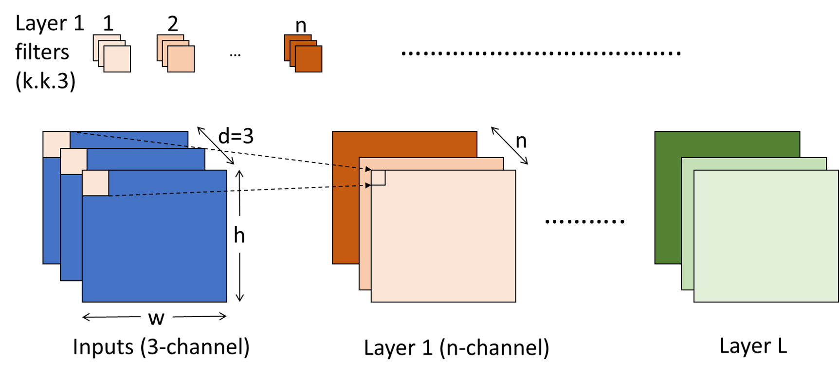
Figure 1: Deep Convolutional Neural Network

Sparse CNNs result in significantly less compute (e.g., 4-9x) and data (e.g., 2-3x) by avoiding zeros. In doing so, the reuse patterns remain the same though the reuse counts decrease. However, implementing sparse vector-vector multiplication, the key primitive in sparse CNNs, is challenging.

2.1 Sparse CNN acceleration at small scale

The central issue with small-scale two-sided sparse architectures is efficient implementation of the key primitive – the sparse tensor-tensor multiplication. Figure 2 shows a processing element (PE) which is the building block for multiplication. For sparse tensors, the primitive involves finding the matching non-zero positions in the two tensors. The sparse data representation impacts the efficiency of this matching. EIE [21] and SCNN [36] employ Compressed Sparse Row (CSR) whereas SparTen [20] employs a bit-mask representation. CSR representation uses two vectors: one for the non-zero offsets and another for the non-zero values, whereas the bit-mask representation uses a fixed-size bit mask to indicate zero and non-zero positions, and a vector for the non-zero values. The latter enables efficient matching via simple ANDing, prefix sum and priority encoder circuits. ExTensor [25] proposes using CAMs for the matching. SCNN avoids this matching altogether for unit-stride convolutions via an unusual dataflow but incurs overheads resulting in intra- and inter-PE idling [20, 40]. In SparTen, an output unit examines consecutive output channels, discards any zeros due to the Rectifier Linear Unit (ReLU) and writes the sparse output tensor, as per the chosen representation, to the on-chip cache or off-chip memory.

In general, the architectures group many lanes, each of which includes a PE, into a cluster (Figure 2). In each cluster, each lane holds a different filter (lanes are analogous to our IFGCs). Each input map is broadcast to the lanes to capture input map reuse across the filters. Multiple input maps are processed to capture filter reuse across the input maps. (Filter and input map reuse are symmetric and interchangeable.) The clusters may operate asynchronously with respect to each other. Alternatively, the filter or input map broadcast may cover multiple clusters.

Buffering, load balancing, and on-chip bandwidth demand are key inter-related aspects of the architectures. The broadcasts save on-chip bandwidth by avoiding repeated refetches of filters and input maps from the cache but require some buffering. While dense architectures like the TPU can be efficient in buffering, sparsity makes such efficiency challenging. Dense CNNs are highly regular where every cell in a tensor is guaranteed to contribute in a fixed pattern to the product. The TPU captures this regularity in a systolic architecture (proposed in [32]) where each MAC requires only a few buffers. Specifically, the TPU accumulates the partial product for a product along a column of the systolic array passing down the partial product to the next cell (near neighbor) achieving efficient pipelined parallelism within a tensor-tensor multiplication. Thus, each MAC needs to buffer data only for a simple scalar-scalar multiplication, so that the MACs in a systolic column share the buffers needed for a product. Sparse CNNs, however, are irregular in that each non-zero scalar in a tensor contributes to the product only if there is a match in the other tensor. Consequently, the buffering in sparse accelerators has to increase to accommodate this uncertainty. Sparse accelerators cannot efficiently pipeline the multiplication due to the uncertainty, which disallows any buffer partitioning and forces the architectures to replace intra-multiplication pipelined parallelism with inter-multiplication parallelism. While abundant, the latter disallows sharing of the buffers.

In addition to the buffering for the filters and input maps, the output maps also need buffering. However, because an entire tensor-tensor multiplication produces only a single cell in the output tensor, output buffers tend to be smaller than the filter and input map buffers.

While the filter and input map broadcasts save bandwidth, load imbalance across the lanes and clusters due to sparsity increases the need for buffering the broadcast data. Due to uneven sparsity, a leading lane or cluster may run far ahead of the lagging lane or cluster. Either all the broadcast data within this gap must be buffered or the broadcast must be stalled until the lagging entity has caught up enough to free up some buffers. Reasonable buffering often implies frequent stalls due to the implicit barriers imposed by the broadcasts in the presence of load imbalance. A third option is to have the lagging entity refetch the broadcast data that could not be buffered. However, this option degrades bandwidth. Architectures exploiting bit sparsity  [12] propose to alleviate load imbalance at the bit level by dynamically stealing work from adjacent lanes. However, such work-stealing involves dynamically scheduling and routing input and output values at high speeds which is complex to implement for full values. SparTen [20] proposes a load balancing scheme which either co-locates and serializes two filters on one PE causing underutilization at large scales or employs a permutation network in each cluster that is hard to scale up (discussed in Section 3.3.3).

2.2 Challenges in scaling up sparse CNN acceleration

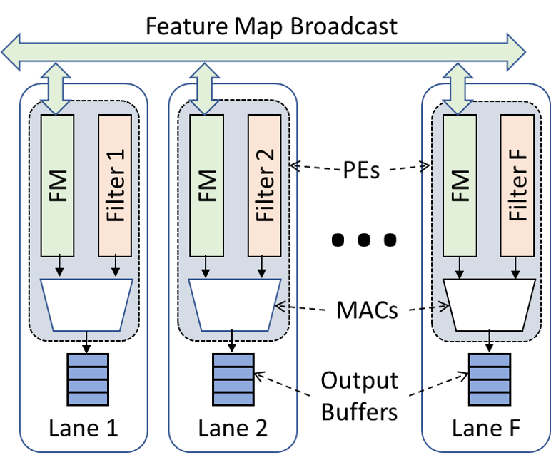
Figure 2: A cluster in a small-scale sparse CNN accelerator

At small scales (e.g., 1K MACs), broadcasting within a cluster and employing asynchronous clusters work well with reasonable on-chip buffering (e.g., around 1-KB buffering per MAC amounts to only 1 MB total on-chip buffers). However, the inter-related issues of buffering, load imbalance, and bandwidth demand make it significantly challenging to scale up sparse architectures to the scales of dense architectures. For instance, naively scaling up SparTen’s asynchronous clusters with 32 MACs each to 32K MACs would require IK clusters, requiring 1K refetches or more than 32-MB on-chip buffering (in addition to a large cache). On the other hand, synchronizing the clusters via broadcasts to limit the required bandwidth and buffering would incur steep load imbalance at such extreme scales. Given that the filters are shared across the lanes (one axis) and the input maps are shared across the clusters (another axis), all the MACs (e.g., 32K at large scale) have to stay load-balanced to avoid excessive buffering or bandwidth demand.

3 BARISTA

Recall from Section 1 that to address the above problems, BARISTA proposes barrier-free execution at large scale (i.e., no broadcasts). Note that barrier-free does not mean wait-free; BARISTA incurs minimal waiting to achieve within 6% of ideal performance. To prevent buffering and on-chip bandwidth requirements from exploding due to the lack of broadcasts, BARISTA makes the following contributions: First, to reduce the on-chip bandwidth BARISTA employs telescoping request combining for input maps and snarfing for filters (on-chip bandwidth demand). Second, to avoid barriers among the PEs between consecutive input maps per filter, BARISTA employs output buffer coloring so that processing of different input maps may overlap across the PEs (input feature map barrier avoidance). Third, to alleviate systematic load balance among a node’s PEs handling different filter parts, BARISTA employs simple round-robin assignment of work to the PEs (intra-filter load balance). Further, to load balance across the filters, BARISTA employs a variant of SparTen’s Greedy Balancing (inter-filter load balance) in software. A common theme among these techniques is that because of the scale they use either simple hardware or software.

Like previous architectures, BARISTA exposes a simple interface for matrix-vector ($C\leftarrow Ax+y$) and matrix-matrix multiplications ($C\leftarrow A\times B)$. The interface linearizes tensors, which may be laid out non-contiguously in memory, into vectors for the relevant operations.

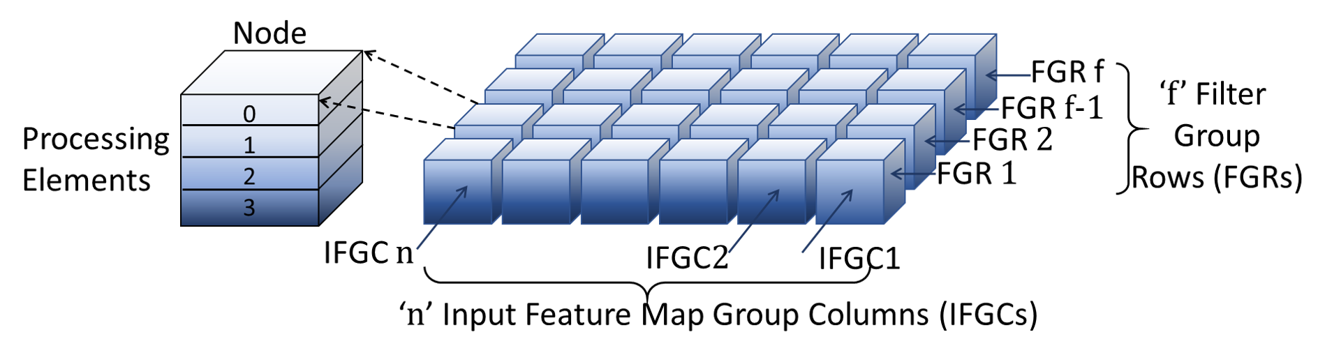
Figure 3: Compute organization in BARISTA

3.1 BARISTA organization

To achieve good reuse of input maps and filters, BARISTA employs much larger clusters. Each of BARISTA’s clusters is organized as a three-dimensional compute grid of filter group rows (FGRs) and input map group columns (IFGCs) intersecting at nodes each of which comprises multiple processing elements (PEs) (Figure 3). For instance, a cluster comprises 64 FGRs and 32 IFGCs and 4 PEs per node for a total of 8K PEs, achieving high within-cluster reuse. To match the TPU’s 32K MACs (two clusters), BARISTA requires four clusters which are connected to an on-chip cache. Each FGR works mostly on one filter at a time (possibly straying to a few filters due to barrier freedom) and a different input map per node. Similarly, each IFGC works mostly on one input map at a time and a different filter per node. Employing multiple PEs per node reduces buffering by sharing a node’s buffers among its PEs and improves load imbalance by requiring fewer IFGCs with lower spread of work variation. While the buffering decreases with more PEs per node, using many PEs would result in them running out of work due to sparsity. Assigning more work per IFGC to feed more PEs would leave some IFGCs idle (abundant parallelism but also vast compute resources).

Like other architectures, BARISTA partitions filters and input maps into chunks for practical hardware granularity (e.g., 128 tensor cells). To ensure that one output tensor cell is computed entirely at a node, all the chunks of one full input map tensor and one full filter tensor are handled at the node. Processing of consecutive output channels is assigned to consecutive nodes in an IFGC (Figure 3). This assignment simplifies output handling, similar to previous proposals (e.g.,  [8, 20]). Each input map chunk is processed by the filters in an IFGC (Figure 3). Similarly, each filter chunk is processed by the input maps in an FGR. Thus, there is spatial reuse of each input map (filter) across the nodes in an IFGC (FGR). If there are more input maps than the IFGCs, then the filters in an IFGC are reused over time across different input maps; similarly for more filters than FGRs. The input map chunk and filter chunk are buffered at each node.

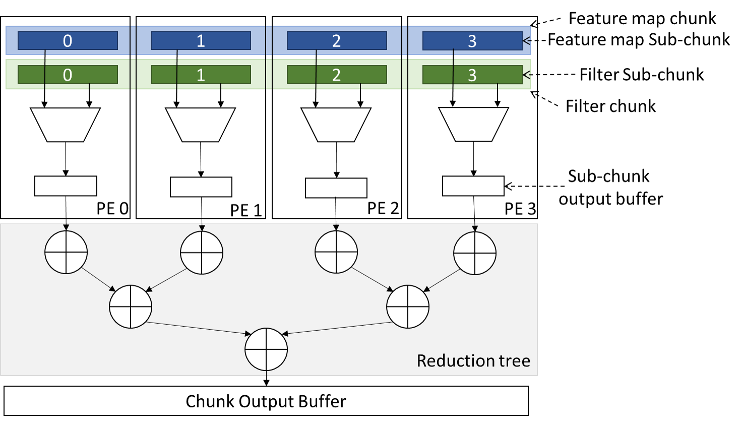
Figure 4: Node organization

At each node, the PEs statically partition the input map chunk into sub-chunks (Figure 4). Each PE multiplies its sub-chunk with the corresponding filter sub-chunk and accumulates the result in a sub-chunk output buffer. The sparse sub-chunk multiplication may be accomplished by any of the previously-proposed methods (Section 2.1). Due to sparsity, the PEs may complete at different times. When all of a node’s PEs are done, the results are reduced through a small adder tree in the node to the final chunk output which is buffered at the node (Figure 4). When all the chunks of the tensors being multiplied are complete, the output cell is complete. When all the output cells in an IFGC are complete, a conversion unit forms the output in the chosen representation after discarding any zeros due to ReLU and writes back to an on-chip cache. If there is temporal reuse of the same filter (input map) over several input maps (filters), then the chunk output for each input map (filter) is buffered separately at the node. A positive side-effect of the sub-chunks is that the PE circuitry (e.g., prefix sum and priority encode [20] or CAMs [25]) would be smaller than that for the full chunks.

The basic organization double-buffers the filters and input maps to hide latency. However, if some nodes within IFGCs or FGRs are lagging and have not consumed their buffers, then each of those nodes would refetch the filters or inputs when its buffers are free. Next, we discuss our techniques for on-chip bandwidth demand, load imbalance, and buffering.

3.2 Cutting on-chip bandwidth demand

To eliminate the barriers induced by synchronous broadcasts, BARISTA proposes to employ asynchronous fetches of the input maps and filters. To reduce the ensuing bandwidth demand, BARISTA employs snarfing and telescoping request combining for the filters and input maps, respectively. These schemes are based on the observation that if the filters and input feature maps are reasonably load-balanced, most of the nodes in an IFGC would be working on the same input map chunk (with different filters). Similarly, most of the nodes in an FGR would be working on the same filter chunk (with different input maps). This in-sync progress implies that even without (implicit) barriers the nodes in an IFGC would request the same input map chunks at about the same time; and the nodes in an FGR would request the same filter chunks at about the same time.

Filters, being read-only for inference, can be load-balanced offline whose cost can be amortized over numerous inferences, but not input maps which are produced dynamically. Assuming our variant of SparTen’s offline inter-filter load balancing (discussed later), the filters have much lower spread of density variation than the input maps. Consequently, while the nodes in an IFGC stray less from each other in terms of progress, there is more straying among the nodes in an FGR. Fortunately, a common dichotomy in most architectures between filters and input maps is that each filter is reused with many inputs both spatially (in each FGR) and temporally (e.g., 16 times in each FGR node) whereas each input is reused only spatially with many filters (in each IFGC). The roles of inputs and filters may be reversed but the dichotomy exists nevertheless because we hold one of either the filters or input maps and cycle through the other. As such, the filters are reused more and hence are fetched less often. Therefore, the straying in an FGR does not result in excessive filter refetching.

Due to this dichotomy, simple snarfing suffices for filters so that when a node in an FGR makes a filter request, the other nodes that have empty filter buffers snarf the response (Figure 6). The remaining nodes refetch the filter with the possibility of snarfing amongst themselves. The snarfing incurs only around two refetches per filter due to the high filter reuse.

Though to a lesser extent than the FGR nodes, the nodes in an IFGC do stray. Figure 5 plots on the X axis the progress of input maps in an IFGC from AlexNet Layer 3 and the completion times on the Y axis. The filters are sorted by completion time. The figure shows the filters with two input maps, consecutive in time (the first input starts at time 20,000 and the second at 23,500). For the lower input map, a few fastest nodes are quite ahead whereas a majority of the nodes stray only gradually from each other followed in time by fewer slower nodes. The rest of the figure is explained next.

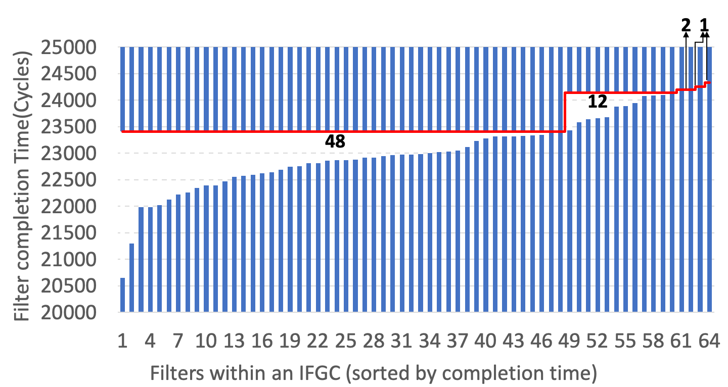
Figure 5: Telescoping request combining

For input map requests, simple snarfing would require many more refetches than those of the filters because of less reuse. Instead, we observe that the IFGC nodes’ requests that occur nearly together in time can be combined while introducing little delay. However, the straying implies that combining all the requests together would delay the leading nodes which may be the lagging nodes for later input maps. That is, with unlimited buffering, for instance, the leading nodes would gain time with the current input maps and would spend the gains on future input maps for which the nodes lag, achieving good load balancing. Implicit barriers between consecutive input maps, due either to synchronous broadcasts or to all-request combining, prevent this transfer of time and hurt performance. Consequently, BARISTA reaches a compromise by matching the request combining to the tapering nature of the number of nodes in the straying groups. Instead of combining sets of the same number of requests, BARISTA combines telescoping numbers of requests (e.g., out of the 64 requests for the lower input map in Figure 5, BARISTA combines the first 48 requests, the next 12, the next two, and leaves the last two uncombined). Even though this example implies five refetches, often the requests in the next set arrive before the first set response increasing the effective combining count. Thus, in practice, the example configuration makes only three refetches on average. See Figure 6 (the buffers are explained later). This scheme requires, per IFGC, (a) a counter for the requests and (b) a simple state machine to effect the telescoping count sequence.

3.3 Tackling load imbalance

While PEs, IFGCs, and FGRs all incur load imbalance, each IFGC operates on one input map and multiple filters which may incur load imbalance. As mentioned before, while filters are load-balanced offline (i.e., inter-filter load balance), input maps are not. Next, we address the input map load imbalance and intra-filter load imbalance within a node.

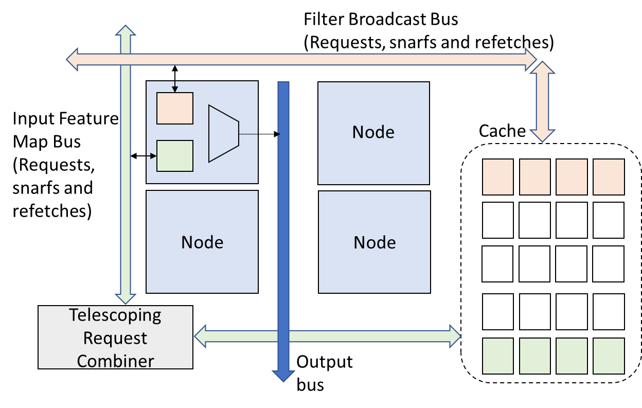
Figure 6: Data transfer with snarfing and request combining

3.3.1 Input feature map barrier avoidance:

To achieve good filter reuse, a given filter at a node in an FGR processes many input feature maps separated by node-local barriers. We avoid these barriers which impose input map load imbalance overhead. That is, some PEs in the node can move on to the next input map while others are still working on the previous input map. Because the input maps are different, the chunk outputs are buffered separately. Previously, however, the input maps are processed sequentially without overlap so that all the PE’s outputs go to the same output buffer at any given time. Now, the PEs’ outputs can concurrently go to different outputs. Accordingly, our coloring scheme provides different sub-chunk output buffers for each PE (Figure 4). Further, the coloring matches the inputs with the sub-chunk output buffers using simple tags (e.g., 4-bit tags for 16 input maps and output buffers). Fortunately, the extra sub-chunk buffering cost is minimal because multiplying entire tensors produces just one output cell (e.g., 4 bytes per node).

While coloring addresses input map load imbalance within a node, the imbalance across IFGCs is harder to address due to the dynamic nature of the input maps. Processing many input maps per filter for filter reuse (e.g., 16 input maps) helps to lessen this imbalance over a large amount of work.

3.3.2 Intra-filter load balance:

While buffer sharing among a node’s PEs reduces buffering, a major source of load imbalance among the node’s PEs is the static partitioning and assignment of a filter’s sub-chunks to the PEs. The assignment is susceptible to systematic load imbalance across the PEs. For instance, if a dense sub-chunk of a filter chunk is assigned to a PE to be reused for several input maps over time then the PE would lag another that is assigned a sparser sub-chunk. Here, we assume that a denser filter sub-chunk would result in more multiplication work than a sparser one (i.e., sub-chunk density is a proxy for multiplication work), even though the work depends on the number of the matching non-zero positions in the filter and input map, and not the number of non-zero positions in the filter alone. The latter PE has to wait for the former before the input map buffer is released and the next input map can be fetched (temporal reuse of the filter over several input maps). To address this issue, BARISTA exploits the diversity in the density of sub-chunks of the input map chunks processed by an IFGC. Accordingly, BARISTA employs dynamic round-robin assignment of filter sub-chunks to the PEs over consecutive input maps chunks assuming that the intra-chunk density distribution among the sub-chunks would even out over multiple chunks. For example. PE $i$ handles sub-chunk $i$ in chunk $0$, sub-chunk $i+1$ in chunk $1$, and so on. This assignment requires simple demultiplexing of the sub-chunks into the node’s buffers (e.g., 1-4 demultiplexor for 4 PEs per node).

3.3.3 Inter-filter load balance:

The filters in an IFGC may vary in density causing load imbalance across the IFGC’s nodes. SparTen’s Greedy Balancing software variant (GB-S) [20] addresses this load imbalance by offline sorting the whole filters by density and co-locating pairs of filters at each node, the densest and sparsest, the second densest and second sparsest, and so on. The sorting and co-location ensure that the total work per node of the co-located filters is similar across the IFGC’s nodes. Such sorting scrambles the output channels. To match the scrambled output channels with the filters’ weights in the next layer, this scheme statically reorders the next layer’s weights in software. Thus, the offline processing proceeds layer by layer, occurs once, and is amortized over all inferences. This software scheme works well at small scale but serializes the filter pairs at a node leading to idling of nodes at larger scales. SparTen also proposes a software-hardware hybrid variant (GB-H) which sorts the filters at the chunk granularity. To reorder the output channels for each chunk, GB-H employs a per-cluster permutation network which needs to support only low bandwidth for SparTen’s small clusters but much higher bandwidths for BARISTA’s larger clusters.

As such, BARISTA employs a GB-S variant (hence, not claimed as a contribution) which performs whole-filter sorting but not co-location. As discussed in Section 3.4, the increased buffering absorbs some of the non-systematic load imbalance due to the lack of chunk-level sorting. However, the lack of co-location causes systematic load imbalance. The nodes in an IFGC with the denser filters lag behind those with the sparser filters. To address this issue, BARISTA alternates the filter-to-node assignment in an IFGC between increasing and decreasing orders of filter density for consecutive input maps. This assignment produces two mutually-reverse orderings of the output channels for consecutive input maps (i.e., only two fixed permutations as opposed to any permutation in GB-H). To reorder the output channels, the conversion unit (Section 3.1) requires a 2-1 multiplexor to choose between the two orderings as opposed to GB-H’s full permutation network.

3.4 Hierarchical buffering

Assuming the bit-mask representation (Section 2.1), the input map and filter each uses a 128-bit mask and a 128-byte block for data values. If there were only one PE per node, the cluster would have 128 IFGCs and 64 FGRs for 8K PEs. Assuming 128 IFGCs, the output data would be 128 1-byte cells. In a 128-PE FGR without coloring, the total buffering would be ((128 bits + 128 bytes) * 2 (input and filter) + 1 byte (output)) * 128 (PEs) * 2 (double-buffering) = 72.25 KB (i.e., 578 B per PE). For 64 FGRs in a cluster and four clusters, the total would be around 18 MB. Using four PEs to share a node’s buffering brings this total down to 4.5 MB.

This amount of buffering, however, exposes significant load imbalance especially because the PEs exploit intra-chunk parallelism shrinking the compute time per chunk (e.g., assuming an average 5x reduction in work due to sparsity, 128-bit mask and 4 PEs imply around 6 multiplications per chunk). Such short compute times are susceptible to load imbalance due to even small variances among the IFGCs and FGRs. Because the input maps are spatially-reused within the IFGCs and the filters are spatially-reused within the FGRs, all the 32 IFGCs and 64 FGRs (i.e., 2K nodes in BARISTA’s cluster) need to stay load-balanced to avoid waiting due to unavailable buffers. This requirement is challenging due to the scale involved.

In addition to load balancing (Section 3.3), more buffering of the filters and input maps would help. However, naively increasing the buffering to recover performance results in buffering bloat (e.g., 8x). Because the filters are reused more than the input maps (the dichotomy in Section 3.2), the former need less buffering (e.g., 3x instead of 8x). However, filter reuse requires more output buffering (e.g., 16x is typical).

To reduce the input map buffering, using narrower buffers degrades the cache bandwidth due to narrow fetches. Instead, BARISTA proposes hierarchical buffering, which enables both high cache bandwidth via chunk-wide fetches into a few chunk-wide, shared input map buffers (at each IFGC) and low buffering by employing narrower sub-chunk-wide buffers at each node (see Figure 6). While the shared buffers’ cost is amortized over the entire IFGC, the per-node buffers impose most of the overall buffering cost. However, fewer per-node buffers cause more waiting in telescoping used by IFGC nodes to cut input map refetches from the shared buffers to the per-node buffers. Fortunately, because the shared buffers are shared only within an IFGC and not globally, the buffers can afford some refetches from the nodes (e.g., 2-3 refetches per IFGC). Consequently, less than 8x per-node buffering for input maps suffices (e.g., 3x instead of 8x). In a 64-node IFGC, the total buffering is [(128 bits + 128 bytes) (input) * 16 (shared buffer depth)] + [(128 bits + 128 bytes) (filter) + (32 bits + 32 bytes) (input/PE) * 4 (PEs/node)] * 64 (nodes) * 3 (per-node buffering) + [1 byte (coloring sub-chunk output/PE) * 4 (PEs/node) + 1 byte (chunk output/node)] * 64 (nodes) * 16 (output buffering) = 61.25 KB (i.e., 245 B per PE). For 32 IFGCs per cluster and four clusters, the total is 7.66 MB.

4 Methodology

To evaluate BARISTA, we build a cycle-level simulator and synthesize an ASIC from a System Verilog implementation.

Table 1: Benchmarks (* 2 inception C modules)

Bench-	# layers	filter	input map
mark		density	density
AlexNet	5	0.368	0.473
ResNet18	17	0.336	0.486
Inception-v4	20*	0.570	0.317
VGGNet	13	0.334	0.446
ResNet50	49	0.421	0.384

Benchmarks: To obtain the sparse versions of the networks in Table 1, we apply pruning and retraining to the networks’ filters, as described by the original work [23]. As recommended, we retrain the filters to try to recover the original accuracy without pruning. The resulting sparsity is in line with previously-reported results [23]. We use a mini-batch of 32, int8 representation, 224x224 inputs from ImageNet [14], and SparTen’s bit mask-based sparse representation [20].

Simulated systems: To isolate the basic impact of two-sided sparsity, we simulate each of a dense accelerator, a one-sided sparse architecture (e.g., Cnvlutin), and three two-sided sparse architectures – SCNN (tile size 6x6), SparTen, and BARISTA (see Table 2). We scale up the previous sparse architectures from their proposed scale by simply adding more clusters. To avoid underutilization in SCNN, each cluster operates on an independent image in the batch. The main point of this paper is that achieving reuse via broadcasts induces implicit barriers which raise the inter-related issues of load imbalance, buffering and bandwidth demand. To study this point we simulate other systems. While SCNN employs synchronous broadcasts across all clusters, SCNN incurs overheads related to its Cartesian product approach in addition to the barrier costs. To isolate the barrier cost of broadcasts, we simulate a broadcast-based scheme, called Synchronous which employs intra-cluster broadcasts (8K-MAC clusters similar to BARISTA). SparTen, which employs asynchronous refetches across its small clusters (and local broadcasts within each cluster), incurs high bandwidth at scale (numerous clusters). To isolate the impact of BARISTA’s optimizations, we simulate BARISTA-no-opts which has BARISTA’s organization but not the optimizations (refetches within its large clusters). To evaluate the amount of buffering needed to avoid barrier costs, we simulate a broadcast scheme with unlimited buffering, called Unlimited-buffer. Note that what matters is the granularity of the broadcasts; not the cluster size. Broadcasts to many PEs (within one large cluster or across many small clusters) expose load imbalance or incur buffering, whereas broadcasts to fewer PEs (in a subset of a large cluster or a small cluster) or no broadcasts at all incur on-chip bandwidth.

We simulate the one-sided architecture, SparTen and BARISTA based on SparTen’s PEs and bit-mask representation using 128-byte chunks. BARISTA uses 64 FGRs and 32 IFGCs to balance filter-reuse and feature-map reuse. Because this paper’s goal is not a design-space exploration, we choose reasonable parameters for BARISTA based on light exploration - the best parameters would only improve BARISTA. Table 2 lists the hardware parameters. Except for unlimited-buffer, all the architectures have similar resources, such as PEs, buffering, and off- and on-chip bandwidth, to isolate the impact of the architectural differences without confounding resource disparities. As discussed in Section 2.1, a TPU-like dense accelerator needs only 8 bytes of buffering per MAC to achieve the highest performance. Adding more buffers will hurt the accelerator’s energy without improving performance. Sparse architectures need more buffering than dense architectures but smaller caches due to eliding zeros (around 2.5x smaller). Due to their regularity, dense architectures need only a few banks to achieve the highest performance. For energy, we use estimates based on our RTL implementation.

Table 2: Hardware parameters

Architecture	MACs/cluster	# clusters	buffer/MAC
Dense	16K	2	8 B
One-sided	32	1K	819 B
SCNN	1K	32	1.63 KB
SparTen	32	1K	993 B
Synchronous	8K	4	993 B
BARISTA	8K	4	245 B
BARISTA-no-opts	8K	4	245 B
Unlimited buffer	8K	4	infinite
Architecture	cache size	cache banks
Dense	24 MB	8
Sparse	10 MB	32

Area, Power, Clock speed estimates from ASIC synthesis: We synthesize an ASIC for our System Verilog implementation of one BARISTA cluster using Synopsys’s Design Compiler and the 45 nm technology FreePDK45 library [35]. Lacking a memory compiler, the library synthesizes the buffers using inefficient flip-flops instead of SRAM arrays. To avoid this artificial overhead, we separately model the area and power of the buffers using CACTI 6.5 [30]. For CACTI power estimation, we conservatively assume the activity to be one read and one write every cycle.

5 Results

Our results show the following: (1) performance comparison of BARISTA against other schemes, (2) execution time breakdown for all the schemes to explain their performance, (3) isolation of the impact of BARISTA’s techniques, (4) energy comparison, and (5) area, power, and clock speed estimates from an ASIC synthesis of our RTL implementation.

5.1 Performance

We compare the performance of a dense architecture (Dense), a one-sided sparse architecture (e.g., Cnvlutin) where only the input maps are sparse (One-sided), SCNN (a two-sided sparse architecture), SparTen (a two-sided architecture), Synchronous (a two-sided architecture which employs broadcasts), BARISTA, and Ideal which has unlimited bandwidth and buffering. In addition, because SparTen uses 1.9X more area than BARISTA (Section 5.6), we also include an iso-area variant of SparTen (SparTen-Iso). Both One-sided and SparTen asynchronously refetch the data without broadcasts. Our key claim is that at the extreme scales of BARISTA, achieving reuse via broadcasts induces implicit barriers which raise the inter-related issues of load imbalance, buffering and bandwidth demand. The barriers expose load imbalance (shown by Synchronous) whereas (a) asynchronous refetches would impose severe bandwidth costs (shown by SparTen and later by BARISTA-no-opts) and (b) buffering the broadcasts would require inordinate amount of buffering (evaluated next). Our comparison illustrates these issues.

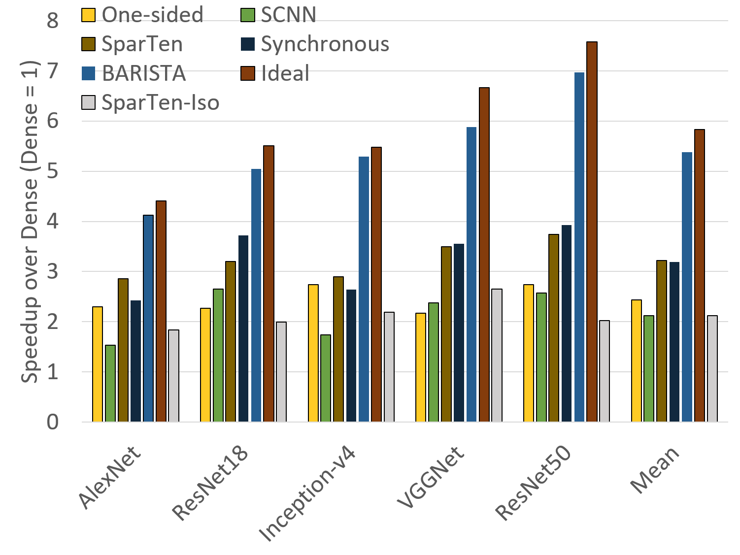
Figure 7: Speedup

Figure 7 shows the performance of these schemes normalized to that of Dense (Y-axis). The X-axis shows the benchmarks and their geometric mean. To see the trends clearly, the benchmarks are ordered by increasing sparsity and hence opportunity (Table 1). One-sided improves over Dense by exploiting one-sided sparsity. Though SCNN targets two-sided sparsity, its Cartesian product approach imposes significant overheads [40, 20]. These overheads drag SCNN behind One-sided in many benchmarks, despite SCNN targeting more sparsity than One-sided. SparTen improves over One-sided by exploiting two-sided sparsity while avoiding SCNN’s overheads. SparTen’s asynchronous clusters minimize barrier costs but impose significant bandwidth demand which Synchronous avoids via broadcasts. However, Synchronous incurs implicit barriers which push Synchronous slightly behind SparTen on average, though the barrier costs are worse than the bandwidth penalty in some benchmarks and vice versa in others.

BARISTA alleviates both SparTen’s bandwidth demand via snarfing and telescoping request combining (BARISTA’s bandwidth reduction schemes) and Synchronous’s load imbalance via coloring, dynamic round robin, and the inter-filter load balancing variant (BARISTA’s load balancing techniques). Consequently, BARISTA performs better than SparTen and Synchronous, achieving more than 5.4x average speedup over Dense and within 6% of Ideal. BARISTA’s speedup trends across the benchmarks match the sparsity (opportunity) trends.

While BARISTA performs 1.7x better than SparTen, this comparison obscures the fact that SparTen, when scaled up to 32K MACs occupies significantly more area than BARISTA (shown later in Section 5.6). In an equal-area comparison to SparTen-Iso, BARISTA achieves 2.5x speedup.

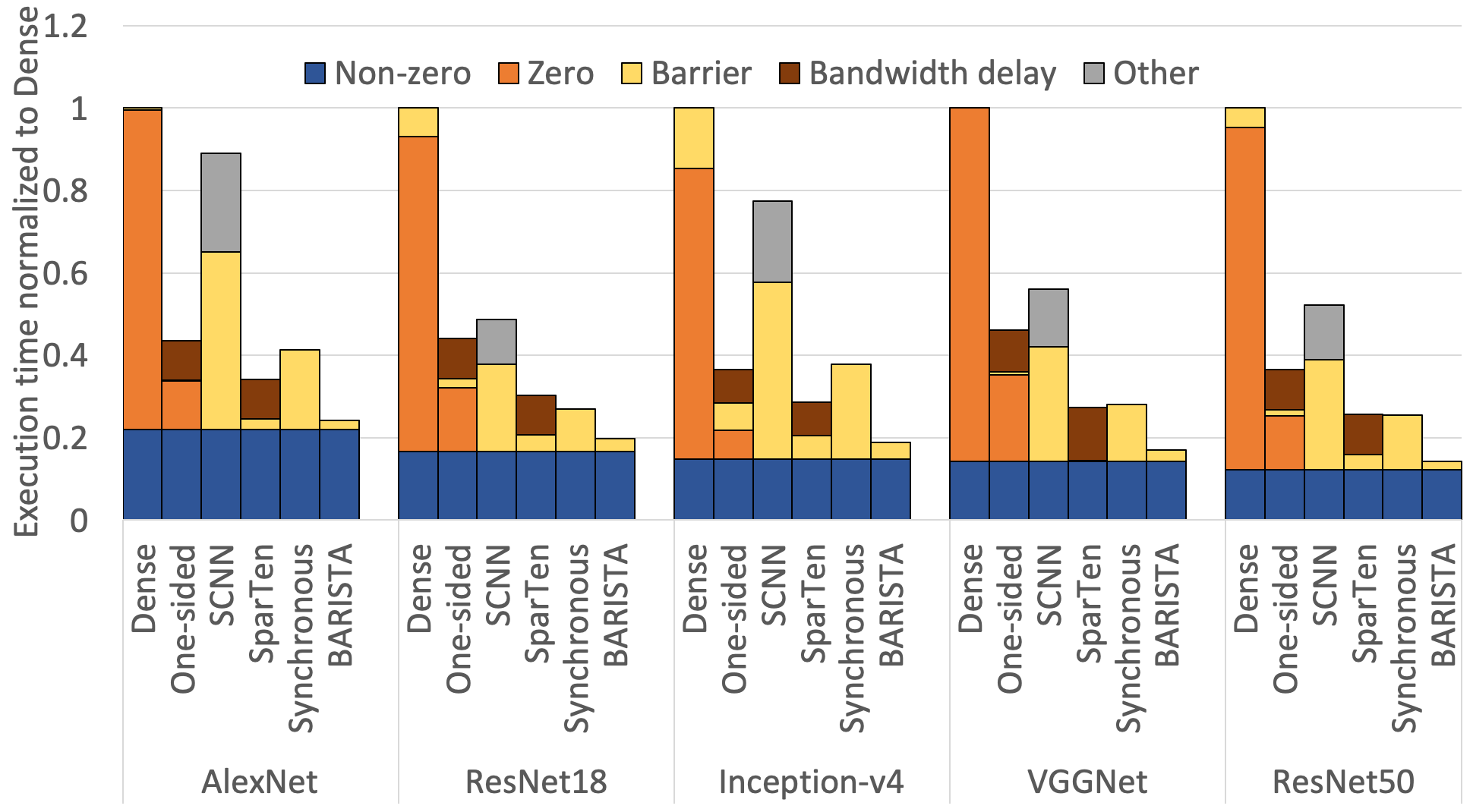
Figure 8: Execution time breakdown

To study the amount of buffering required to avoid both barrier costs and refetch bandwidth, we simulated BARISTA by turning off the telescoping request combining and turning on unlimited buffering in a configuration called called Unlimited-buffer (Section 4). We found that in all the benchmarks Unlimited-buffer needs more than 24x buffering (i.e., more than 185 MB) to achieve the same performance as BARISTA.

5.2 Execution time breakdown

To understand the speedups, Figure 8 breaks down the above architectures’ execution time for our benchmarks normalized to that of Dense. The execution time components are: non-zero computation, zero computation, barrier loss, bandwidth-imposed delay, and other (explained below). As expected, Dense incurs many zero computations which is the motivation for sparse architectures. By exploiting one-sided sparsity One-sided incurs fewer zero computations than Dense but One-sided’s refetches incur bandwidth delay. SCNN exploits two-sided sparsity to eliminate zero computations but incurs significant overheads due to (1) its Cartesian product approach as mentioned above (shown as "other") as well as (2) barriers induced by its broadcasts. The two-sided SparTen incurs low barrier cost due to local broadcasts only within its small clusters but high bandwidth delays due to asynchronous refetches by the clusters. On the other hand, Synchronous incurs barrier cost due to the broadcasts within its clusters. Finally, thanks to its bandwidth-reduction and load-balancing schemes, BARISTA incurs only some residual bandwidth delay and barrier cost.

5.3 Energy

Figure 9 shows the energy for Dense, Ones-sided, SparTen (with asynchronous refetches), and BARISTA normalized to that of Dense on the Y axis, and the benchmarks and their mean on the X axis. SCNN performs worse than One-sided and is hard to model in enough detail for meaningful energy results. Therefore, we do not show SCNN. Further, our RTL synthesis tool chain does not estimate DRAM energy which cannot be normalized easily against the accelerator’s energy. Therefore, we show compute and memory energies separately. We further break down (a) compute energy into zero, non-zero and data access (cache and buffers) components, and (b) memory energy into zero and non-zero components.

Dense’s compute energy is dominated by zero compute and data access which includes both zeros and non-zeros. One-sided incurs higher compute energy than Dense because sparse computation requires more energy (finding the non-zero positions, as described in Section 2.1). In the case of One-sided, this extra energy is incurred for both non-zeros and zeros (zeros are not elided in one of the two input tensors). Though Dense incurs access energy for both zeros and non-zeros, Dense achieves high reuse due to its regularity and therefore makes the fewest accesses possible (Section 2.1). On the other hand, One-sided both accesses the zeros that are not elided, and does not achieve as good reuse as Dense. As such, One-sided’s clusters refetch data many times, incurring high data access energy (filters or input maps are symmetrical). Thus, One-sided’s sparsity is not enough to reduce compute significantly but is enough to disrupt reuse and force refetches.

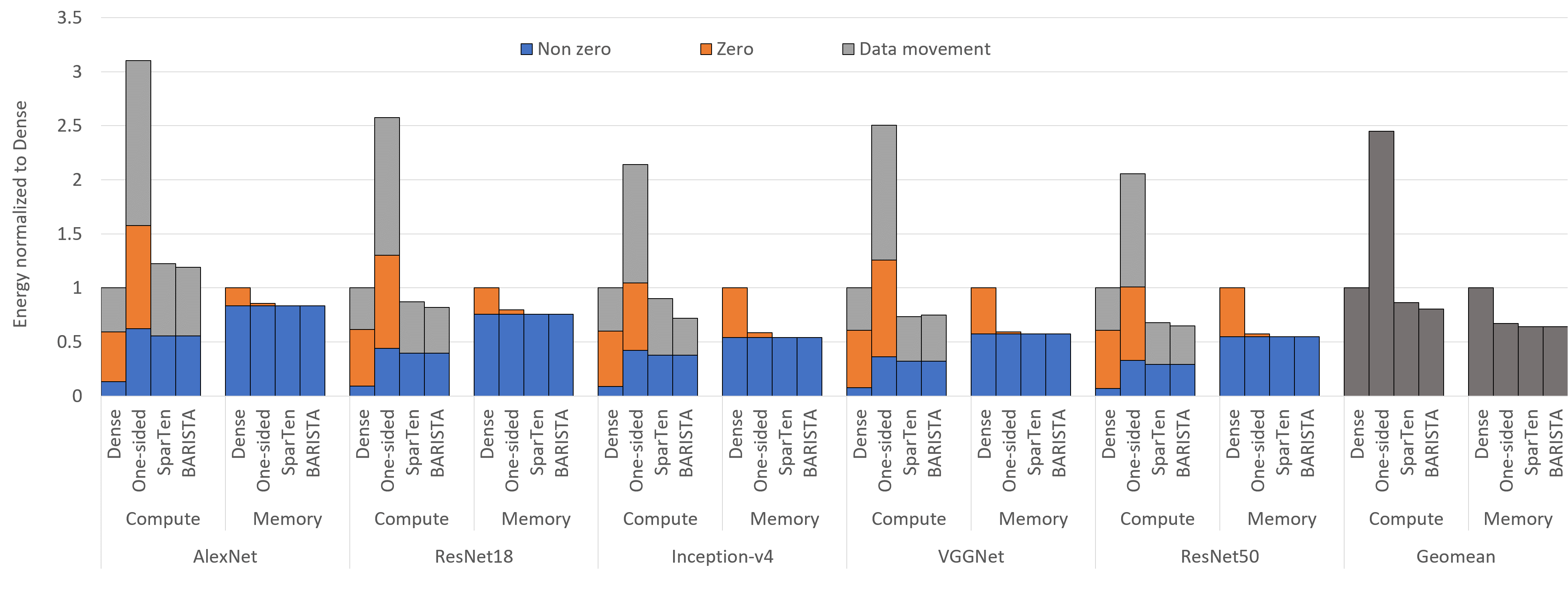
Figure 9: Energy

By exploiting two-sided sparsity, SparTen entirely avoids zero compute but incurs higher non-zero compute energy because two-sided sparse computation takes even more energy than one-sided sparse computation (finding the matching non-zero positions in the two input tensors as opposed to the non-zero positions in one input tensor). Like One-sided, SparTen also incurs more data access energy than Dense. However, unlike One-sided, SparTen entirely avoids accessing zeros to achieve lower data access energy than One-sided. As a result of the opposing effects of no zero compute or access but higher non-zero compute and access, SparTen’s net compute energy starts out being more than that of Dense at the left end of the graph and ends up being less than that of Dense at the right end (i.e., as sparsity increases from left to right). Finally, BARISTA’s compute energy is identical to that of SparTen because they employ the same PE circuitry (Section 3.1). Further, BARISTA achieves only slightly lower data access energy than SparTen because the former’s shared buffer energy offsets the latter’s refetch energy. The impact of SparTen’s refetches in the form of bandwidth delay causes a wider gap between SparTen and BARISTA in performance (Figure 7) than in energy (Figure 9) because of the naturally synchronous (bursty) nature of the refetches. The bursts cause significant queuing due to cache bank conflicts which BARISTA avoids by controlling the refetches. Like SparTen, BARISTA’s compute energy also decreases with increasing sparsity from left to right.

Unlike Dense’s compute energy, its memory energy is dominated by non-zeros because compute volume decreases quadratically over sparsity whereas memory volume decreases only linearly. One-sided reduces memory energy by eliminating input map zeros. In memory energy, input maps dominate filters which have high reuse and low memory traffic due to batching. Consequently, the two-sided SparTen and BARISTA improve only slightly over One-sided in memory energy despite eliminating both input map and filter zeros. Though One-sided, SparTen, and BARISTA incur some overhead in non-zero memory energy due to the bit masks and pointers for sparse data, the overhead is invisible. As the sparsity increases from left to right, the savings from zeros exceed the penalty from non-zeros so that BARISTA’s memory energy decreases.

5.4 Isolating BARISTA’s techniques

Figure 10 isolates the impact of BARISTA’s techniques on performance. The Y axis shows the speedup over Dense for our benchmarks (including their geometric mean). The graph starts on the left with Sparten for reference and an initial BARISTA configuration without any of the optimizations (BARISTA-no-opts). Like SparTen, this configuration (1) already includes SparTen’s GB-S for inter-filter load balancing (the variant described in Section 3.3.3) and (2) employs asynchronous refetches which incur bandwidth delay. To this configuration, we progressively add one at a time telescoping request combining, coloring, hierarchical buffering, and dynamic round robin assignment which results in the full BARISTA design. Unsurprisingly, the rise from Dense to SparTen corresponds to exploiting sparsity, which is the central opportunity for all sparse architectures. Due to its higher on-chip bandwidth demand than SparTen, BARISTA-no-opts performs worse than SparTen which while being asynchronous like BARISTA-no-opts uses bandwidth-saving broadcasts within its clusters unlike BARISTA-no-opts. Every one of BARISTA’s techniques contribute more or less similarly to fill the gap between BARISTA-no-opts and BARISTA. The only exception is in inception-v4 which has low data volume, and hence low in-chip bandwidth pressure, so that adding telescoping to BARISTA-no-opts does not show any improvements.

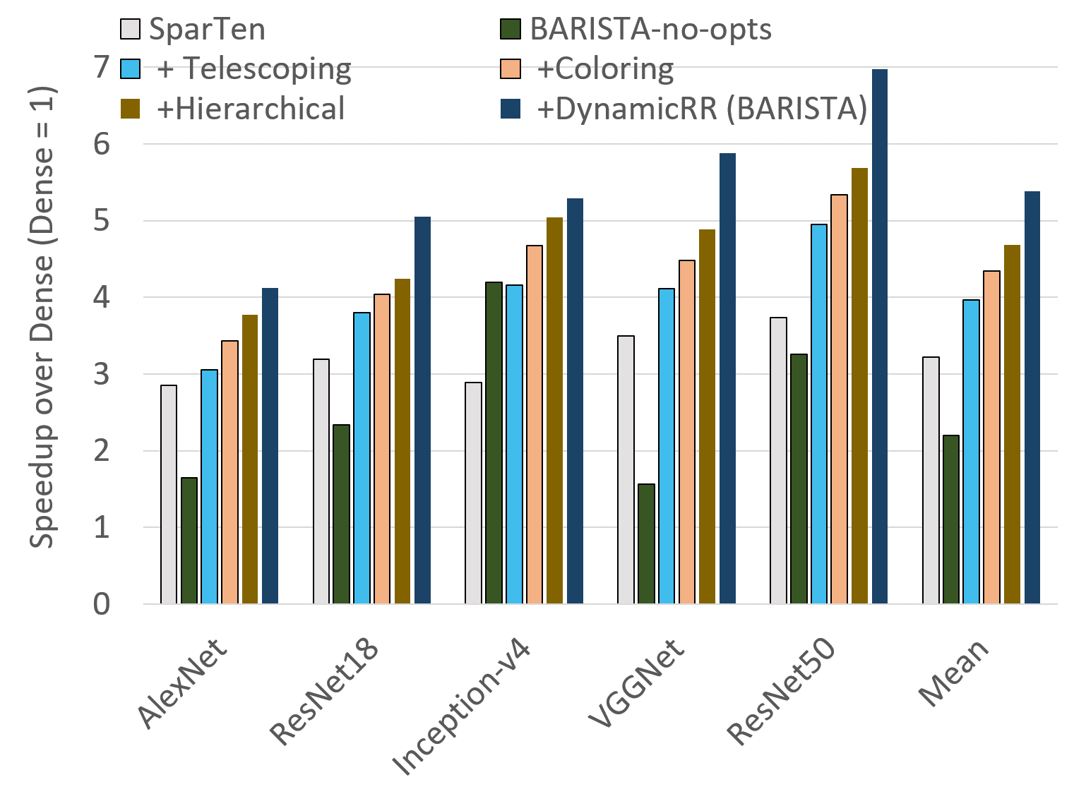
Figure 10: Isolating BARISTA’s techniques

5.5 Sensitivity to Buffer Size

BARISTA’s snarfing and telescoping request combining are key optimizations for reducing the refetches due to the barrier-free straying of FGRs and IFGCs. Figure 11 shows refetches (Y-axis) averaged over all layers, and over all feature maps and filters for each benchmark (groups of bars along the X-axis) as we apply BARISTA’s optimizations and as we vary the buffer size (bars within each group). Without the optimizations (leftmost bar), the average number of refetches is dominated by the feature-map refetches; filter refetches, though included, are much fewer because filters are reused 16 times over multiple inputs. There is a dramatic drop in the number of refetches when BARISTA’s optimizations are applied. Increasing buffer sizes (4 MB, 6 MB and 8 MB) result in progressively fewer refetches. We found that though bandwidth demand continues to drop with more buffering, there was no significant performance benefit beyond 8 MB (default).

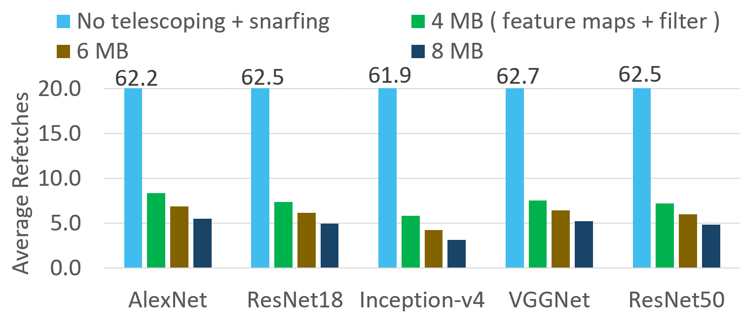
Figure 11: Sensitivity to Buffer Size

5.6 ASIC synthesis results

Table 3 shows the area and power estimates using 45-nm technology for four BARISTA clusters with 8K PEs each. We scaled up SparTen to 1K 32-PE clusters. These estimates show that BARISTA’s area and power are 89% and 26% smaller than those of SparTen; both designs achieve 1-GHz clock speed. SparTen incurs higher area and power due to larger buffers (Table 2) as well as control and bus interfaces replicated for 1K clusters. Otherwise, SparTen and BARISTA have identical area and power for prefix sum, priority encoders and MACs, as expected. Prefix sum and priority encoders are smaller here for both BARISTA and SparTen than in the original SparTen paper [20] due to sub-chunk-based circuits (32 B versus 128 B), as discussed in Section 3.1. In contrast, Dense achieves lower total area and power than BARISTA due to smaller buffers and the lack of the sparsity circuitry. Dense’s cache is larger to accommodate the non-sparse data. Overall, BARISTA achieves 5.4x higher performance than Dense at the cost of 38% more area and 2.05x more power.

6 Related work

Table 3: Area and power estimates for BARISTA (45 nm)

	BARISTA		SparTen		Dense
	Area	Pwr	Area	Pwr	Area	Pwr
	(mm2)	(W)	(mm2)	(W)	(mm2)	(W)
Buffers	73.3	73.4	137.7	98.3	38.6	46.7
Prefix	43.6	43.1	43.6	43.1	-	-
Priority	8.7	3.7	8.7	3.7	-	-
MACs	44.2	33.7	44.2	33.7	44.2	33.7
Other	20.2	12.3	110.8	20.8	1.5	1.2
Cache	22.9	3.6	22.9	4.5	69.8	1.4
Total	212.9	170	402.7	214.9	154.1	83

There are many optimizations for dense architectures, focusing on compute [19, 41, 28, 26, 17, 32], memory [9, 33, 16], and reuse [8, 5]. In-memory architectures [6, 42, 39, 10] leverage analog logic for dense matrix multiplication but must contend with the well-known analog-related issues of noise, scalability, and process variation. One-sided sparse architectures target sparsity in either filters or feature maps but not both [4, 44, 21, 12] and two-sided architectures [36, 20, 25] exploit sparsity in the convolutional layers to reduce compute and data volumes. We have discussed SCNN and SparTen extensively. ExTensor [25] proposes hierarchical representations for sparse tensors. EIE [21] targets two-sided sparsity only in the fully-connected layers but performs similarly to one-sided schemes due MAC idling for zeros in the filters. Diffy [34] extends sparsity by exploiting small differences in the values. Other work proposes CPU instruction-set support (a) to index efficiently into a hierarchical bitmap representation for sparse tensors [27] and (b) to store the data in memory after removing zeros while the computation does not elide zeros [2].

Bit-sparse architectures [3, 12, 40] leverage Booth encoding to elide zero bits. Unlike two-sided value-sparse architectures, the bit-sparse architectures incur overheads to store and transfer zero values. Further, the fundamental issues of load imbalance, reuse, and buffering remain for bit-sparse architectures as well (e.g., implicit barrier after every set of products in Bit Laconic and conservative buffering of uncompressed values before Booth encoding). PermDNN [13] converts sparse filters into permuted diagonal matrices [18] only for fully-connected layers. CirCNN [15] uses block-circulant matrices for filters but requires complex FFT hardware and does not capture all sparsity.

Other papers constrain sparsity to be coarse-grained to match hardware granularity [43], or by forcing zeros in contiguous [45] or the same [29] positions in groups of filters. In contrast, BARISTA is based on Deep Compression [22] which prunes each filter value independent of granularity and other filters. Such pruning carefully maintains accuracy by retraining whereas the constrained sparsity proposals either do not not evaluate accuracy on high-accuracy deep models [43, 45] or lower accuracy (e.g., from 93.75% to 93% [29] which is a 12% increase in inaccuracy).

In High-Performance Computing (HPC), many implementations improve sparse BLAS libraries’ performance over CPUs [46, 7]. However, the implementations remain significantly slower than dense accelerators like GPUs.

7 Conclusion

Scaling up two-sided sparse architectures is challenging because alleviating the implicit barrier costs induced by broadcasts to achieve reuse raises the inter-related issues of load imbalance (e.g., keeping all 32K MACs load-balanced), buffering, and on-chip bandwidth demand. To address these issues, we proposed barrier-free large-scale sparse tensor accelerator (BARISTA). BARISTA (1) is the first architecture for scaling up sparse CNN accelerators; (2) reduces on-chip bandwidth demand by telescoping request combining the input map requests and snarfing the filter requests; (3) reduces buffering via basic buffer sharing and avoids the ensuing barriers between consecutive input maps by coloring the output buffers; (4) load balances a filter chunks among a node’s PEs via dynamic round-robin work assignment; and (5) employs hierarchical buffering for high cache bandwidth via wide fetches into shared buffers and narrower, private buffers at the compute. Our simulations show that, on average, BARISTA performs 5.4x, 2.2x, 1.7x, and 2.5x better and achieves 19%, 67%, 7%, and 7% lower compute energy than a dense, a one-sided, a naively-scaled two-sided, and an iso-area two-sided architecture, respectively. Using 45-nm technology, ASIC synthesis of our RTL implementation for four clusters of 8K PEs each reports 1-GHz clock speed, 213 mm² area and 170 W power. We leave applying BARISTA to deep neural networks other than CNNs and sparse linear algebra in HPC to future work. As such, BARISTA is an attractive option for large-scale sparse tensor computation due to its at-scale high performance and efficiency.

References

- [1] “Nvidia introduces drive agx orin — advanced, software-defined platform for autonomous machines | nvidia newsroom,” https://nvidianews.nvidia.com/news/nvidia-introduces-drive-agx-orin-advanced-software-defined-platform-for-autonomous-machines, (Accessed on 02/14/2020).
- [2] B. Akin, Z. A. Chishti, and A. R. Alameldeen, “Zcomp: Reducing dnn cross-layer memory footprint using vector extensions,” in Proceedings of the 52Nd Annual IEEE/ACM International Symposium on Microarchitecture, ser. MICRO ’52. New York, NY, USA: ACM, 2019, pp. 126–138. [Online]. Available: http://doi.acm.org/10.1145/3352460.3358305
- [3] J. Albericio, A. Delmas, P. Judd, S. Sharify, G. O’Leary, R. Genov, and A. Moshovos, “Bit-pragmatic deep neural network computing,” in Proceedings of the 50th Annual IEEE/ACM International Symposium on Microarchitecture, MICRO 2017, Cambridge, MA, USA, October 14-18, 2017, 2017, pp. 382–394. [Online]. Available: http://doi.acm.org/10.1145/3123939.3123982
- [4] J. Albericio, P. Judd, T. H. Hetherington, T. M. Aamodt, N. D. E. Jerger, and A. Moshovos, “Cnvlutin: Ineffectual-neuron-free deep neural network computing,” in 43rd ACM/IEEE Annual International Symposium on Computer Architecture, ISCA 2016, Seoul, South Korea, June 18-22, 2016, 2016, pp. 1–13. [Online]. Available: http://dx.doi.org/10.1109/ISCA.2016.11
- [5] M. Alwani, H. Chen, M. Ferdman, and P. Milder, “Fused-layer cnn accelerators,” in 49th Annual IEEE/ACM International Symposium on Microarchitecture (MICRO), 2016.
- [6] A. Ankit, I. E. Hajj, S. R. Chalamalasetti, G. Ndu, M. Foltin, R. S. Williams, P. Faraboschi, W.-m. W. Hwu, J. P. Strachan, K. Roy, and D. S. Milojicic, “Puma: A programmable ultra-efficient memristor-based accelerator for machine learning inference,” in Proceedings of the Twenty-Fourth International Conference on Architectural Support for Programming Languages and Operating Systems, ser. ASPLOS ’19. New York, NY, USA: ACM, 2019, pp. 715–731. [Online]. Available: http://doi.acm.org/10.1145/3297858.3304049
- [7] N. Bell and M. Garland, “Implementing sparse matrix-vector multiplication on throughput-oriented processors,” in Proceedings of the Conference on High Performance Computing Networking, Storage and Analysis, Nov 2009, pp. 1–11.
- [8] Y.-H. Chen, T. Krishna, J. Emer, and V. Sze, “14.5 eyeriss: An energy-efficient reconfigurable accelerator for deep convolutional neural networks,” in 2016 IEEE International Solid-State Circuits Conference (ISSCC), Jan 2016, pp. 262–263.
- [9] Y. Chen, T. Luo, S. Liu, S. Zhang, L. He, J. Wang, L. Li, T. Chen, Z. Xu, N. Sun, and O. Temam, “Dadiannao: A machine-learning supercomputer,” in Proceedings of the 47th Annual IEEE/ACM International Symposium on Microarchitecture, ser. MICRO-47. Washington, DC, USA: IEEE Computer Society, 2014, pp. 609–622. [Online]. Available: http://dx.doi.org/10.1109/MICRO.2014.58
- [10] P. Chi, S. Li, C. Xu, T. Zhang, J. Zhao, Y. Liu, Y. Wang, and Y. Xie, “Prime: A novel processing-in-memory architecture for neural network computation in reram-based main memory,” in Proceedings of the 43rd International Symposium on Computer Architecture, ser. ISCA ’16. Piscataway, NJ, USA: IEEE Press, 2016, pp. 27–39. [Online]. Available: https://doi.org/10.1109/ISCA.2016.13
- [11] R. Csongor, “Tesla raises the bar for self-driving carmakers | the official nvidia blog,” https://blogs.nvidia.com/blog/2019/04/23/tesla-self-driving/, (Accessed on 02/14/2020).
- [12] A. Delmas, P. Judd, D. M. Stuart, Z. Poulos, M. Mahmoud, S. Sharify, M. Nikolic, and A. Moshovos, “Bit-tactical: Exploiting ineffectual computations in convolutional neural networks: Which, why, and how,” CoRR, vol. abs/1803.03688, 2018. [Online]. Available: http://arxiv.org/abs/1803.03688
- [13] C. Deng, S. Liao, Y. Xie, K. K. Parhi, X. Qian, and B. Yuan, “Permdnn: Efficient compressed dnn architecture with permuted diagonal matrices,” in 2018 51st Annual IEEE/ACM International Symposium on Microarchitecture (MICRO), Oct 2018, pp. 189–202.
- [14] J. Deng, W. Dong, R. Socher, L.-J. Li, K. Li, and L. Fei-Fei, “ImageNet: A Large-Scale Hierarchical Image Database,” in CVPR09, 2009.
- [15] C. Ding, S. Liao, Y. Wang, Z. Li, N. Liu, Y. Zhuo, C. Wang, X. Qian, Y. Bai, G. Yuan, X. Ma, Y. Zhang, J. Tang, Q. Qiu, X. Lin, and B. Yuan, “Circnn: Accelerating and compressing deep neural networks using block-circulant weight matrices,” in Proceedings of the 50th Annual IEEE/ACM International Symposium on Microarchitecture, ser. MICRO-50 ’17. New York, NY, USA: ACM, 2017, pp. 395–408. [Online]. Available: http://doi.acm.org/10.1145/3123939.3124552
- [16] Z. Du, R. Fasthuber, T. Chen, P. Ienne, L. Li, T. Luo, X. Feng, Y. Chen, and O. Temam, “Shidiannao: Shifting vision processing closer to the sensor,” in Proceedings of the 42Nd Annual International Symposium on Computer Architecture, ser. ISCA ’15. New York, NY, USA: ACM, 2015, pp. 92–104. [Online]. Available: http://doi.acm.org/10.1145/2749469.2750389
- [17] J. Fowers, K. Ovtcharov, M. Papamichael, T. Massengill, M. Liu, D. Lo, S. Alkalay, M. Haselman, L. Adams, M. Ghandi, S. Heil, P. Patel, A. Sapek, G. Weisz, L. Woods, S. Lanka, S. K. Reinhardt, A. M. Caulfield, E. S. Chung, and D. Burger, “A configurable cloud-scale dnn processor for real-time ai,” in Proceedings of the 45th Annual International Symposium on Computer Architecture, ser. ISCA ’18. Piscataway, NJ, USA: IEEE Press, 2018, pp. 1–14. [Online]. Available: https://doi.org/10.1109/ISCA.2018.00012
- [18] N. E. Gibbs, W. G. Poole, Jr., and P. K. Stockmeyer, “A comparison of several bandwidth and profile reduction algorithms,” ACM Trans. Math. Softw., vol. 2, no. 4, pp. 322–330, Dec. 1976. [Online]. Available: http://doi.acm.org/10.1145/355705.355707
- [19] V. Gokhale, A. Zaidy, A. X. M. Chang, and E. Culurciello, “Snowflake: An efficient hardware accelerator for convolutional neural networks,” in 2017 IEEE International Symposium on Circuits and Systems (ISCAS), May 2017, pp. 1–4.
- [20] A. Gondimalla, N. Chesnut, M. Thottethodi, and T. N. Vijaykumar, “Sparten: A sparse tensor accelerator for convolutional neural networks,” in Proceedings of the 52Nd Annual IEEE/ACM International Symposium on Microarchitecture, ser. MICRO ’52. New York, NY, USA: ACM, 2019, pp. 151–165. [Online]. Available: http://doi.acm.org/10.1145/3352460.3358291
- [21] S. Han, X. Liu, H. Mao, J. Pu, A. Pedram, M. A. Horowitz, and W. J. Dally, “Eie: Efficient inference engine on compressed deep neural network,” in 2016 ACM/IEEE 43rd Annual International Symposium on Computer Architecture (ISCA), June 2016, pp. 243–254.
- [22] S. Han, H. Mao, and W. J. Dally, “Deep compression: Compressing deep neural network with pruning, trained quantization and huffman coding,” in 4th International Conference on Learning Representations, ICLR 2016, San Juan, Puerto Rico, May 2-4, 2016, Conference Track Proceedings, 2016. [Online]. Available: http://arxiv.org/abs/1510.00149
- [23] S. Han, J. Pool, J. Tran, and W. Dally, “Learning both weights and connections for efficient neural network,” in Advances in Neural Information Processing Systems 28, C. Cortes, N. D. Lawrence, D. D. Lee, M. Sugiyama, and R. Garnett, Eds. Curran Associates, Inc., 2015, pp. 1135–1143. [Online]. Available: http://papers.nips.cc/paper/5784-learning-both-weights-and-connections-for-efficient-neural-network.pdf
- [24] K. He, X. Zhang, S. Ren, and J. Sun, “Deep residual learning for image recognition,” CoRR, vol. abs/1512.03385, 2015. [Online]. Available: http://arxiv.org/abs/1512.03385
- [25] K. Hegde, H. Asghari-Moghaddam, M. Pellauer, N. Crago, A. Jaleel, E. Solomonik, J. Emer, and C. W. Fletcher, “Extensor: An accelerator for sparse tensor algebra,” in Proceedings of the 52Nd Annual IEEE/ACM International Symposium on Microarchitecture, ser. MICRO ’52. New York, NY, USA: ACM, 2019, pp. 319–333. [Online]. Available: http://doi.acm.org/10.1145/3352460.3358275
- [26] N. P. Jouppi, C. Young, N. Patil, D. Patterson, G. Agrawal, R. Bajwa, S. Bates, S. Bhatia, N. Boden, A. Borchers, R. Boyle, P.-l. Cantin, C. Chao, C. Clark, J. Coriell, M. Daley, M. Dau, J. Dean, B. Gelb, T. V. Ghaemmaghami, R. Gottipati, W. Gulland, R. Hagmann, C. R. Ho, D. Hogberg, J. Hu, R. Hundt, D. Hurt, J. Ibarz, A. Jaffey, A. Jaworski, A. Kaplan, H. Khaitan, D. Killebrew, A. Koch, N. Kumar, S. Lacy, J. Laudon, J. Law, D. Le, C. Leary, Z. Liu, K. Lucke, A. Lundin, G. MacKean, A. Maggiore, M. Mahony, K. Miller, R. Nagarajan, R. Narayanaswami, R. Ni, K. Nix, T. Norrie, M. Omernick, N. Penukonda, A. Phelps, J. Ross, M. Ross, A. Salek, E. Samadiani, C. Severn, G. Sizikov, M. Snelham, J. Souter, D. Steinberg, A. Swing, M. Tan, G. Thorson, B. Tian, H. Toma, E. Tuttle, V. Vasudevan, R. Walter, W. Wang, E. Wilcox, and D. H. Yoon, “In-datacenter performance analysis of a tensor processing unit,” in Proceedings of the 44th Annual International Symposium on Computer Architecture, ser. ISCA ’17. New York, NY, USA: ACM, 2017, pp. 1–12. [Online]. Available: http://doi.acm.org/10.1145/3079856.3080246
- [27] K. Kanellopoulos, N. Vijaykumar, C. Giannoula, R. Azizi, S. Koppula, N. M. Ghiasi, T. Shahroodi, J. G. Luna, and O. Mutlu, “Smash: Co-designing software compression and hardware-accelerated indexing for efficient sparse matrix operations,” in Proceedings of the 52Nd Annual IEEE/ACM International Symposium on Microarchitecture, ser. MICRO ’52. New York, NY, USA: ACM, 2019, pp. 600–614. [Online]. Available: http://doi.acm.org/10.1145/3352460.3358286
- [28] A. Krizhevsky, I. Sutskever, and G. E. Hinton, “Imagenet classification with deep convolutional neural networks,” in Advances in Neural Information Processing Systems 25, F. Pereira, C. J. C. Burges, L. Bottou, and K. Q. Weinberger, Eds. Curran Associates, Inc., 2012, pp. 1097–1105. [Online]. Available: http://papers.nips.cc/paper/4824-imagenet-classification-with-deep-convolutional-neural-networks.pdf
- [29] H. T. Kung, B. McDanel, and S. Q. Zhang, “Packing sparse convolutional neural networks for efficient systolic array implementations: Column combining under joint optimization,” CoRR, vol. abs/1811.04770, 2018. [Online]. Available: http://arxiv.org/abs/1811.04770
- [30] H. labs, “Cacti 6.5,” https://www.hpl.hp.com/research/cacti/.
- [31] Y. Lecun, L. Bottou, Y. Bengio, and P. Haffner, “Gradient-based learning applied to document recognition,” Proceedings of the IEEE, vol. 86, no. 11, pp. 2278–2324, Nov 1998.
- [32] D. D. Lin, S. S. Talathi, and V. S. Annapureddy, “Fixed point quantization of deep convolutional networks,” in Proceedings of the 33rd International Conference on International Conference on Machine Learning - Volume 48, ser. ICML’16. JMLR.org, 2016, pp. 2849–2858. [Online]. Available: http://dl.acm.org/citation.cfm?id=3045390.3045690
- [33] D. Liu, T. Chen, S. Liu, J. Zhou, S. Zhou, O. Teman, X. Feng, X. Zhou, and Y. Chen, “Pudiannao: A polyvalent machine learning accelerator,” in Proceedings of the Twentieth International Conference on Architectural Support for Programming Languages and Operating Systems, ser. ASPLOS ’15. New York, NY, USA: ACM, 2015, pp. 369–381. [Online]. Available: http://doi.acm.org/10.1145/2694344.2694358
- [34] M. Mahmoud, K. Siu, and A. Moshovos, “Diffy: a déjà vu-free differential deep neural network accelerator,” in 2018 51st Annual IEEE/ACM International Symposium on Microarchitecture (MICRO), Oct 2018, pp. 134–147.
- [35] NCSU, “Freepdk45,” https://www.eda.ncsu.edu/wiki/FreePDK45:Contents#Current_Version.
- [36] A. Parashar, M. Rhu, A. Mukkara, A. Puglielli, R. Venkatesan, B. Khailany, J. Emer, S. W. Keckler, and W. J. Dally, “Scnn: An accelerator for compressed-sparse convolutional neural networks,” in Proceedings of the 44th Annual International Symposium on Computer Architecture, ser. ISCA ’17. New York, NY, USA: ACM, 2017, pp. 27–40. [Online]. Available: http://doi.acm.org/10.1145/3079856.3080254
- [37] O. Russakovsky, J. Deng, H. Su, J. Krause, S. Satheesh, S. Ma, Z. Huang, A. Karpathy, A. Khosla, M. S. Bernstein, A. C. Berg, and F. Li, “Imagenet large scale visual recognition challenge,” CoRR, vol. abs/1409.0575, 2014. [Online]. Available: http://arxiv.org/abs/1409.0575
- [38] A. Samajdar, Y. Zhu, P. N. Whatmough, M. Mattina, and T. Krishna, “Scale-sim: Systolic CNN accelerator,” CoRR, vol. abs/1811.02883, 2018. [Online]. Available: http://arxiv.org/abs/1811.02883
- [39] A. Shafiee, A. Nag, N. Muralimanohar, R. Balasubramonian, J. P. Strachan, M. Hu, R. S. Williams, and V. Srikumar, “Isaac: A convolutional neural network accelerator with in-situ analog arithmetic in crossbars,” in Proceedings of the 43rd International Symposium on Computer Architecture, ser. ISCA ’16. Piscataway, NJ, USA: IEEE Press, 2016, pp. 14–26. [Online]. Available: https://doi.org/10.1109/ISCA.2016.12
- [40] S. Sharify, A. D. Lascorz, M. Mahmoud, M. Nikolic, K. Siu, D. M. Stuart, Z. Poulos, and A. Moshovos, “Laconic deep learning inference acceleration,” in Proceedings of the 46th International Symposium on Computer Architecture, ser. ISCA ’19. New York, NY, USA: ACM, 2019, pp. 304–317. [Online]. Available: http://doi.acm.org/10.1145/3307650.3322255
- [41] Y. Shen, M. Ferdman, and P. Milder, “Escher: A CNN accelerator with flexible buffering to minimize off-chip transfer,” in 25th IEEE International Symposium on Field-Programmable Custom Computing Machines (FCCM), 2017.
- [42] L. Song, X. Qian, H. Li, and Y. Chen, “Pipelayer: A pipelined reram-based accelerator for deep learning,” in 2017 IEEE International Symposium on High Performance Computer Architecture (HPCA), Feb 2017, pp. 541–552.
- [43] J. Yu, A. Lukefahr, D. Palframan, G. Dasika, R. Das, and S. Mahlke, “Scalpel: Customizing dnn pruning to the underlying hardware parallelism,” in Proceedings of the 44th Annual International Symposium on Computer Architecture, ser. ISCA ’17. New York, NY, USA: ACM, 2017, pp. 548–560. [Online]. Available: http://doi.acm.org/10.1145/3079856.3080215
- [44] S. Zhang, Z. Du, L. Zhang, H. Lan, S. Liu, L. Li, Q. Guo, T. Chen, and Y. Chen, “Cambricon-x: An accelerator for sparse neural networks,” in The 49th Annual IEEE/ACM International Symposium on Microarchitecture, ser. MICRO-49. Piscataway, NJ, USA: IEEE Press, 2016, pp. 20:1–20:12. [Online]. Available: http://dl.acm.org/citation.cfm?id=3195638.3195662
- [45] X. Zhou, Z. Du, Q. Guo, S. Liu, C. Liu, C. Wang, X. Zhou, L. Li, T. Chen, and Y. Chen, “Cambricon-s: Addressing irregularity in sparse neural networks through a cooperative software/hardware approach,” in 2018 51st Annual IEEE/ACM International Symposium on Microarchitecture (MICRO), Oct 2018, pp. 15–28.
- [46] L. Zhuo and V. K. Prasanna, “Sparse matrix-vector multiplication on fpgas,” in Proceedings of the 2005 ACM/SIGDA 13th International Symposium on Field-programmable Gate Arrays, ser. FPGA ’05. New York, NY, USA: ACM, 2005, pp. 63–74. [Online]. Available: http://doi.acm.org/10.1145/1046192.1046202