Rapid model comparison of equations of state from gravitational wave observation of binary neutron star coalescences

Abstract

The discovery of the coalescence of binary neutron star GW170817 was a watershed moment in the field of gravitational wave astronomy. Among the rich variety of information that we were able to uncover from this discovery was the first non-electromagnetic measurement of the neutron star radius, and the cold nuclear equation of state. It also led to a large equation of state model selection study from gravitational-wave data. In those studies Bayesian nested sampling runs were conducted for each candidate equation of state model to compute their evidence in the gravitational-wave data. Such studies, though invaluable, are computationally expensive and require repeated, redundant, computation for any new models. We present a novel technique to conduct model selection of equation of state in an extremely rapid fashion ($\sim$ minutes) on any arbitrary model. We test this technique against the results of a nested-sampling model selection technique published earlier by the LIGO/Virgo collaboration, and show that the results are in good agreement with a median fractional error in Bayes factor of about 10%, where we assume that the true Bayes factor is calculated in the aforementioned nested sampling runs. We found that the highest fractional error occurs for equation of state models that have very little support in the posterior distribution, thus resulting in large statistical uncertainty. We then used this method to combine multiple binary neutron star mergers to compute a joint-Bayes factor between equation of state models. This is achieved by stacking the evidence of the individual events and computing the Bayes factor from these stacked evidences for each pairs of equation of state.

I Introduction

Neutron stars (NS) are the densest objects that are known to exist in the universe. The structure of isolated nonrotating NS is completely determined by the Tolman-Oppenheimer-Volkoff (TOV) equations Oppenheimer and Volkoff (1939). To solve the TOV equations, however, one needs to know the barotropic equation of state which connects the pressure $(p)$ of nuclear matter at energy density $(\epsilon)$:

$$p=p(\epsilon)\,.$$ (1)

The equation of state of cold matter at extreme density is expected to be universal, i.e., all NS are expected to share the same equation of state. Thus, the equation of state is a fundamental relation of great importance for understanding NS, and more generally, matter at extreme densities. In a typical NS, the central density can, however, reach values as high as ten times the nuclear saturation density Özel and Freire (2016). Such extreme environments cannot be emulated in laboratories. Moreover, limitations in our knowledge of the strong nuclear force, which is partially responsible for the pressure resisting the collapse of a NS due to its gravity, results in inadequate theoretical models of matter at such densities. Thus, the lack of experimental data at high densities and incomplete theoretical understanding of NS models both contribute to the uncertainty in the modeling of the nuclear equation of state. These uncertainties have led to the development of numerous of NS equation of state models.

Solving the TOV equation for these equation of state models allows us to compute the radius of stable nonrotating NS as function of mass. Moreover, it can be shown that there exists one-to-one map between the $p(\epsilon)$ relations of a NS and its mass-radius relations, i.e., there is a one-parameter family of NS based on central pressure Lindblom (1992). Observations of pulsars and measurements of their mass and radius provide us with valuable information about the NS equation of state. Traditionally, this had been the primary avenue of investigation in this field. However, the vast majority of known galactic pulsars ($\sim 3000$) are isolated and only around 10% of systems exist in binaries Manchester et al. (2005); ATNF-CSIRO (2019), for which precise mass measurements are possible. The measurement of a NS’s radius using electromagnetic observation is quite challenging. Most radius measurement techniques for NSs are either based on detecting surface thermal emission, using spectroscopic data to infer the effective temperature assuming isotropic emission models. Alternatively, this could involve the measurement of the general relativistic effects of the NS’s gravity on the thermal emission, for example by projects like Neutron Star Interior Composition Explorer (NICER) NASA (2019); Miller et al. (2019); Riley et al. (2019). However, all these techniques are model-dependent and have multiple sources of systematics Özel and Freire (2016).

Detection of gravitational waves from binary neutron stars (BNS) using ground-based gravitational wave detectors like LIGO Aasi et al. (2015) and Virgo Acernese et al. (2015) presents us with a completely new way of measuring the NS equation of state. It allows us to measure the masses of the NSs directly, and electromagnetic emission model independent measurement of the star’s structure via the tidal deformability. In a coalescing BNS system the spin Poisson (1998) and tidal interactions between the two stars will lead to a change in their shape, and hence changes the quadrupole moment of the binary system. The time-changing induced quadrupole moment results in a faster inspiral as more orbital energy goes into radiation and stellar distortion and this results in observable effects in the gravitational waveform. If the star is subject to a quadrupolar field given by $\mathcal{E}_{\rm ij}$ then the resulting quadrupole moment due to tidal interactions is given by

$$Q_{ij}=-\lambda\mathcal{E}_{ij}\,,$$ (2)

where $\lambda$ is called the tidal deformability of the NS, which is related to the equation of state dependent tidal Love number $k_{2}$ Hinderer (2008) as follows

$$\lambda=\frac{2}{3G}k_{2}R^{5}$$ (3)

where $R$ is the radius of the NS (which, for a given mass, also depends on the equation of state). For a given equation of state and mass of the NS, the tidal deformability, $\lambda$ can be computed by solving the TOV equations along with a differential equation obtained from combining metric perturbation due to external quadrupolar tidal field Flanagan and Hinderer (2008); Hinderer (2008). Therefore, any measurement of the tidal deformability will also lead to constraints on the NS equation of state. This is where gravitational-wave data for coalescing binaries of NSs provide us with an excellent observational window for nuclear matter measurements. By modeling the gravitational waveform while taking into account the tidal deformabilities as extra model parameters Read et al. (2009a); Del Pozzo et al. (2013); Agathos et al. (2015), it is possible to obtain the posterior distribution of the NS masses and tidal deformabilities from Bayesian parameter estimation van der Sluys et al. (2009); Veitch and Vecchio (2010); Raymond et al. (2010); Rodriguez et al. (2014); Veitch et al. (2015) to get posterior distribution on the NS masses and tidal deformabilities. This was conducted for the case of GW170817 by the LIGO/Virgo Collaboration Abbott et al. (2019). Additionally, the constraints on the radii of the NSs were also estimated Abbott et al. (2018); De et al. (2018) after imposing an equation of state insensitive relation between the mass, radius, and tidal deformability. Furthermore, it is possible to parametrize the equation of state using piecewise polytropes or a spectral representation Read et al. (2009b); Lindblom (2010) to infer the equation of state parameters for a given representation Abbott et al. (2018). Finally, nonparametric inference of the cold NS equation of state Landry and Essick (2019); Landry et al. (2020) can help in relaxing the choice of parametrization in describing the equation of state.

All of these aforementioned studies, which are either equation of state agnostic, or which are attempting to reveal the NS equation of state with minimal (albeit varying degrees of) assumptions, are extremely important. One can, however, also make a good argument of studying various equation of state models in the literature that are based on nuclear theory. Analysis of these equation of state models can give us insight into these various theories. There are a few studies in constraining of equation of state models that are motivated from nuclear physics theory Capano et al. (2020); Dietrich et al. (2020), and a large-scale equation of state model selection study has also been conducted by the LIGO/Virgo Collaboration Abbott et al. (2020a) which has investigated 24 equation of state models using Bayesian model selection techniques. Bayesian model selection of NS equation of state requires conducting Bayesian parameter estimation on gravitational-wave data using each model as a prior. Conducting such studies for multiple equation of state is computationally expensive. There is much redundancy in such studies which we want to avoid so that any new equation of state model can be rapidly tested against any other (new or existing) models. We present in this paper a novel technique that allows for reliable and rapid computation of Bayes factors between equation of state models estimated from a single equation of state agnostic Bayesian parameter estimation run on the gravitational-wave data.

The paper is organized as follows: in Sec. II, we briefly review the technique of Bayesian model selection for NS equation of state using gravitational-wave data. In Sec. III we introduce the approximate method for Bayes factor estimation that we use to perform rapid model selection. In Sec. IV we give the details of the parameter estimation runs that are necessary for the application of the approximation method. Then in Sec. V we discuss the results of this technique, where we first show how the method performs compared to the full Bayesian analysis in Abbott et al. (2020a), and then in V.2 we use this technique to demonstrate its ability to stack Bayes factors from multiple BNS mergers in order to make a joint model selection statement. Finally, in Sec. V.3 we apply the method of stacking to obtain a joint Bayes factor between models of NS equation of state as informed by the two observed BNS coalescences, GW170817 and GW190425 Abbott et al. (2021).

II Model selection of equation of state

The time-varying strain at an interferometer due to gravitational wave from a coalescing compact binary system is given by $h(t;m_{1},m_{2},\lambda_{1},\lambda_{2},\vec{\theta})$, where $\vec{\theta}$ is comprised of the spins of the binary, and extrinsic parameters of the source such as its sky-position, the angle of inclination of the binary, the gravitational wave polarization angle, distance to the source, and its phase at coalescence. For this work we have ignored spin contributions to the tidal deformabilities and maximum masses of the binary components. The quantities $m_{i}$ and $\lambda_{i}$, where $i=1,2$, are the masses and tidal deformabilities of the two compact objects. The NS equation of state gives us a map between the masses and the tidal deformability parameters: $\lambda=f(m)$. The interferometer data $d$ in presence of the gravitational wave signal can be expressed as $d(t)=h(t)+n(t)$, where $n(t)$ is the noise in the detector. We can define a likelihood function in the parameter space defined by $(m_{1},m_{2},\lambda_{1},\lambda_{2},\vec{\theta})$ for the observed data as $\mathcal{L}=\mathcal{L}(d\mid m_{1},m_{2},\lambda_{1},\lambda_{2},\vec{\theta})$, which can be used to construct the evidence for the equation of state model defined by $f$,

$$\mathcal{Z}_{f}=\int\mathcal{L}(d\mid m_{1}^{\prime},m_{2}^{\prime},\lambda_{1}^{\prime},\lambda_{2}^{\prime},\vec{\theta}^{\prime})\,p(m_{1}^{\prime},\lambda_{1}^{\prime},m_{2}^{\prime},\lambda_{2}^{\prime}\mid f)\,p(\vec{\theta}^{\prime})\,dm_{1}^{\prime}\,dm_{2}^{\prime}\,d\lambda_{1}^{\prime}\,d\lambda_{2}^{\prime}\,d\vec{\theta}^{\prime}\,,$$ (4)

where the prior for the specific equation of state model is encoded in the probability $p(m_{1},\lambda_{1},m_{2},\lambda_{2}\mid f)$. Computing the value of $\mathcal{Z}_{f}$ and $\mathcal{Z}_{g}$ for two equation of state models $f$ and $g$ and then taking their ratio will give us the Bayes factor $\mathrm{BF}^{f}_{g}=\mathcal{Z}_{f}/\mathcal{Z}_{g}$ between the two models. This technique was employed in Abbott et al. (2020a) and was used to investigate Bayes factors between a multitude of equations of state using the information available from the interferometer data around the time of GW170817 LIGO Scientific Collaboration, Virgo Collaboration (2017). For each of these equations of state the evidence in Eq. (4) was evaluated by conducting a multidimensional Bayesian parameter estimation using nested sampling Skilling (2004). This method, however, is computationally expensive. In the study conducted in Abbott et al. (2020a), the computation of evidence for each equation of state  took $\gtrsim$1 week to finish. Furthermore, if one intends to compare any new equation of state against the existing models, a fresh Bayesian analysis will need to be conducted. This renders the method impractical in the long run (particularly when it must be repeated over a number of gravitational wave events to obtain a joint Bayes factor as we describe in Sec. V.2). Whenever a new equation of state models needs to be included in the study, not only new parameter estimation runs need to be conducted for the new events, but for all events in the past. To address this issue we have developed a method of an evidence-approximation scheme that allows the use of a single Bayesian parameter estimation result to compute the Bayes factor between any two arbitrary equation of state models in a very rapid fashion (typically within minutes). This method allows the user to define any new equation of state model and compare that with any existing model or another new model without having to repeat the full parameter estimation runs. Instead of using the aforementioned parametrization of $(m_{1},m_{2},\lambda_{1},\lambda_{2})$ we re-parametrize the likelihood to $(\mathcal{M},q,\tilde{\Lambda},\delta\tilde{\Lambda})$, where $\mathcal{M}=(m_{1}m_{2})^{3/5}/(m_{1}+m_{2})^{1/5}$ is the chirp mass of the binary, $q=m_{2}/m_{1}$ is the mass ratio, assuming the convention $m_{1}>m_{2}$. $\tilde{\Lambda}$ and $\delta\tilde{\Lambda}$ are tidal parameters defined as

$$\tilde{\Lambda}=\frac{8}{13}\left[(1+7\eta-31\eta^{2})(\Lambda_{1}+\Lambda_{2})+\sqrt{1-4\eta}\,(1+9\eta-11\eta^{2})(\Lambda_{1}-\Lambda_{2})\right]$$ (5)

$$\delta\tilde{\Lambda} = \frac{1}{2}\left[\sqrt{1-4\eta}\left(1-\frac{13272}{1319}\eta+\frac{8944}{1319}\eta^{2}\right)(\Lambda_{1}+\Lambda_{2})+\left(1-\frac{15910}{1319}\eta+\frac{32850}{1319}\eta^{2}+\frac{3380}{1319}\eta^{3}\right)(\Lambda_{1}-\Lambda_{2})\vphantom{\sqrt{1-4\eta}}\right]\,,$$ (6)

where, $\eta=m_{1}m_{2}/(m_{1}+m_{2})^{2}$ is the symmetric mass ratio, and $\Lambda_{1}=G\lambda_{1}[c^{2}/(Gm_{1})]^{5}$ and $\Lambda_{2}=G\lambda_{2}[c^{2}/(Gm_{2})]^{5}$ are dimensionless tidal deformabilities of the two stars, as described in Flanagan and Hinderer (2008); Favata (2014); Wade et al. (2014). This allows us to neatly isolate the dominant tidal contribution to the gravitational waveform, $\tilde{\Lambda}$, from the subdominant contribution of $\delta\tilde{\Lambda}$. We describe the details of the evidence approximation scheme in the next section.

III Evidence approximation scheme

Bayesian model selection among a number of equation of state models requires the computation of the evidence $\mathcal{Z}$ for each model under consideration. The evidence can be computed by methods such as nested sampling  Skilling (2004), but this multidimensional integral must be recomputed for each equation of state model. Here we describe an approximation scheme by which the evidence for each model can be obtained from a low-dimensional integral over a marginalized likelihood function that is constructed from a set of samples drawn from a distribution with a single MCMC sampling.

The approximation method exploits the fact that the chirp mass of a BNS system is extremely well measured from the gravitational wave signal, whereas a second mass parameter, e.g., the mass ratio $q$, will be significantly less constrained. Additionally, the tidal parameter $\tilde{\Lambda}$, first enters the post-Newtonian expansion of the waveform at the 5th post-Newtonian order, while $\delta\tilde{\Lambda}$ first enters the expansion at the 6th post-Newtonian order. The impact of $\delta\tilde{\Lambda}$ is much weaker than the one of $\tilde{\Lambda}$ and can often be neglected.

If we ignore spin contributions, a given equation of state, $E$, defines how the tidal deformabilities are related to the NS mass, $\Lambda_{E}(m)$, as well as a maximum mass $m_{\max,E}$ of a nonrotating NS. We assume that a compact object with $m>m_{\max,E}$ is a black hole (ignoring the possibility of rapidly rotating supramassive NSs) and define $\Lambda_{E}(m)=0$ for $m>m_{\max,E}$. The function $\Lambda_{E}$ then allows us to obtain the functions $\tilde{\Lambda}_{E}(\mathcal{M},q)$ and $\delta\tilde{\Lambda}_{E}(\mathcal{M},q)$ using Eqs. 5 and 6, which determine the parameters $\tilde{\Lambda}$ and $\delta\tilde{\Lambda}$ for a BNS with mass parameters $(\mathcal{M},q)$ Wade et al. (2014). The evidence for equation of state $E$ is then

$$\mathcal{Z}_{E}=\int\mathcal{L}(d\mid\mathcal{M}^{\prime},q^{\prime},\vec{\theta}^{\prime},\tilde{\Lambda}_{E}(\mathcal{M}^{\prime},q^{\prime}),\delta\tilde{\Lambda}_{E}(\mathcal{M}^{\prime},q^{\prime}))\,p(\mathcal{M}^{\prime},q^{\prime})\,p(\vec{\theta}^{\prime})\,d{\mathcal{M}}^{\prime}\,dq^{\prime}\,d\vec{\theta^{\prime}}$$ (7)

and if we marginalize over the parameters $\vec{\theta}$ and express the equation of state constraints as delta-functions, we have

$$\mathcal{Z}_{E}=\int\mathcal{L}(d\mid\mathcal{M}^{\prime},q^{\prime},\tilde{\Lambda}^{\prime},\delta\tilde{\Lambda}^{\prime})\,\delta(\tilde{\Lambda}^{\prime}-\tilde{\Lambda}_{E}(\mathcal{M}^{\prime},q^{\prime}))\,\delta(\delta\tilde{\Lambda}^{\prime}-\delta\tilde{\Lambda}_{E}(\mathcal{M}^{\prime},q^{\prime}))\,p(\mathcal{M}^{\prime},q^{\prime})\,d{\mathcal{M}}^{\prime}\,dq^{\prime}\,d\tilde{\Lambda}^{\prime}\,d\delta\tilde{\Lambda}^{\prime}\,.$$ (8)

The prior distribution over masses $p(\mathcal{M},q)$ is taken to be the same for any equation of state in our approximation, which would neglect astrophysically motivated priors involving mass gaps between the most massive NSs and the least massive black holes.

To obtain the marginal likelihood $\mathcal{L}(d\mid\mathcal{M}^{\prime},q^{\prime},\tilde{\Lambda}^{\prime},\delta\tilde{\Lambda}^{\prime})$ we use well-tested and well-maintained parameter estimation code to compute a posterior distribution: Application of Bayes’s theorem reduces the marginal likelihood to a posterior distribution

$$p(\mathcal{M},q,\tilde{\Lambda},\delta\Lambda\mid d)\propto p(\mathcal{M},q)\mathcal{L}(d\mid\mathcal{M},q,\tilde{\Lambda},\delta\tilde{\Lambda})$$ (9)

where a uniform prior over $\tilde{\Lambda}$ and $\delta\tilde{\Lambda}$ is imposed. This prior in the tidal deformabilities is not physically meaningful: its seemingly unphysical form is needed only to form the correct relation between the posterior distribution and the marginalized likelihood. (The prior over the mass parameters, however, is physically relevant.) However, it must be noted that the prior over deformabilities needs to have support over all possible deformabilities allowed by the equation of state under consideration. As the equation of state dependence appears only in the delta-functions in Eq. (8), the constant of proportionality in Eq. (9) is not equation of state dependent and so is irrelevant for our purposes.

As mentioned earlier it is observed that the posterior distribution is sharply-peaked about some well-measured chirp mass $\mathcal{M}_{0}$, and is largely independent of the subdominant tidal parameter $\delta\tilde{\Lambda}$, so, to a very good approximation

$$p(\mathcal{M},q,\tilde{\Lambda},\delta\tilde{\Lambda}\mid d)\propto p(q,\tilde{\Lambda}\mid d)\,\delta(\mathcal{M}-\mathcal{M}_{0})$$ (10)

where $p(q,\tilde{\Lambda}\mid d)$ is the posterior distribution marginalized over all parameters apart from $q$ and $\tilde{\Lambda}$. Performing the integrals in the evidence, we find

$$\mathcal{Z}_{E}\propto\int p(q^{\prime},\tilde{\Lambda}_{E}(\mathcal{M}_{0},q^{\prime})\mid d)\,dq^{\prime}$$ (11)

i.e., proportional to the line integral over the two-dimensional posterior distribution $p(q,\tilde{\Lambda}\mid d)$ along the curve $\gamma:q\to\tilde{\Lambda}_{E}(q,\mathcal{M}_{0})$ determined by the measured chirp mass $\mathcal{M}_{0}$ and the equation of state $E$. Again, the constant of proportionality is not equation of state dependent and so is irrelevant when computing Bayes factors between different equations of state. The curve $\gamma$ contains the full support of the prior on $q$ which may include values where one or both of the components exceed $m_{\max,E}$, which correspond to neutron-star black-hole binaries and binary black holes.

In our work, we used MCMC stochastic sampling to draw samples from the posterior distribution. We then used a kernel density estimator (KDE) of samples $(q,\tilde{\Lambda})$ drawn from the posterior to obtain a KDE estimate $K(q,\tilde{\Lambda})$ of the function $p(q,\tilde{\Lambda}\mid d)$. The line integral is then written in terms of this estimate as

$$\mathcal{Z}_{E}\propto\int K(q^{\prime},\tilde{\Lambda}_{E}(\mathcal{M}_{0},q^{\prime}))\,dq^{\prime}\,.$$ (12)

Within this approximation scheme, samples from the posterior distribution $p(q,\tilde{\Lambda}\mid d)$ only needs to obtained once (per event) using an equation of state agnostic prior that is uniform over $\tilde{\Lambda}$ and $\delta\tilde{\Lambda}$. Once this has been computed, the evidence for any equation of state model can be efficiently obtained by a one-dimensional line integral of Eq. (12). Because we approximate the posterior distribution with a KDE based on a finite number of samples, this estimation method is subject to sampling uncertainty. We estimate the uncertainty via a bootstrapping approach. From the kernel density we resample the same number of points as the original samples and recompute the evidence using this new set of points. This should give us another instance of the evidence for the same event. Continuing this multiple times we are able to create a distribution of the evidence, which in turn will give us an estimate in the uncertainty of our Bayes factors between two equation of state models. While we believe any biases associated with the point estimate of the evidence ratio to be small, the bootstrapping procedure introduces a bias due to oversmoothing of the posterior. We therefore include a factor of two based on simulation studies (see Appendix) in the error estimates shown in Sec. V in order to render conservative error estimates.

For the results in this work we use a prior that is uniform in $0\leq\tilde{\Lambda}\leq 3000$ and $-500\leq\delta\tilde{\Lambda}\leq 500$. Note that this formally includes (unphysical) negative values of the individual tidal deformabilities $\Lambda_{1}$ and $\Lambda_{2}$. These negative values can lead to issues with waveform generators that fail upon encountering these unphysical points. In this study we used the TaylorF2 waveform Bini et al. (2012) truncated at 5th post-Newtonian order which is a post-Newtonian nonprecessing frequency domain waveform that includes tidal effects. TaylorF2 does not depend on $\delta\tilde{\Lambda}$ and so was largely immune to this issue. The equation of state will affect the gravitational waveform at high frequencies near the point at which the NSs come into contact that are not modeled by the TaylorF2 waveforms. In this work we chose to terminate the waveform at the innermost stable circular orbit (ISCO) Wade et al. (2014). As the detectors are not sensitive at such high frequencies, this arbitrary termination condition is unimportant. A more general approach would be to use an arbitrary prior $p(\Lambda_{1},\Lambda_{2})$ with support only for $\Lambda_{1}\geq 0$ and $\Lambda_{2}\geq 0$ and to divide the posterior distribution by the marginalized prior $p(\tilde{\Lambda})$ (which can be done by reweighting samples drawn from the posterior distribution).

IV Equation of state agnostic parameter estimation runs

The evidence approximation post-processes the Bayesian posterior samples. The current implementation of the method uses an equation of state agnostic MCMC exploration of the 11 dimensional parameter space spanned by $(\mathcal{M},q,\tilde{\Lambda},\delta\tilde{\Lambda},\chi_{1},\chi_{2},d_{L},\theta_{JN},\psi,t,\delta_{c})$. For GW170817 we fix the sky-position at the location of NGC4993. We use LALInference_MCMC from LALsuite library LIGO Scientific Collaboration, Virgo Collaboration (2018) to obtain posterior samples for $\tilde{\Lambda}$ and $q$ as well as the other aforementioned parameters. It implements Metropolis–Hastings algorithm Metropolis et al. (1953); Hastings (1970) with parallel tempering Veitch and Vecchio (2010); Veitch et al. (2015), which modifies the likelihood function $p(d\mid\theta)$ to $p(d\mid\theta)^{1/T}$ for different ‘temperature’ ($T$) chains. In all the examples that follow we choose to use 8 different temperatures from $T=1$ to $T=50$ for each MCMC run. Parallel tempering allows, at higher temperatures efficient ‘global’ exploration of the prior-space, while at the lower temperatures, finer detailed exploration of local space around regions of higher likelihood. During the sampling, each chain swaps samples periodically based on the criteria presented in Ref. Veitch et al. (2015). Samples at the beginning of MCMC known as burn-in period need to be discarded, because they have not explored the entire parameter space and thus they are not guaranteed to be sampled from the posterior. The termination condition can be set to the desired number of samples, however, adjacent samples are usually correlated. We compute autocorrelation time $\tau$ Veitch et al. (2015), and only select effective samples: every $\tau$-th samples after burn-in, which can better sample the posterior as they are independently chosen.

The priors for mass and spin $(\chi)$ that we used for GW170817 are consistent with the priors presented in Ref. Abbott et al. (2020a), specifically, we consider narrow and broad priors on masses and spins. Our choice of the narrow prior is based on BNS observed in our Galaxy. We assume component masses of BNS follow uncorrelated Gaussian distribution with mean $1.33\,M_{\odot}$ and standard deviation $0.09\,M_{\odot}$ Özel and Freire (2016), and employ the sorting convention $m_{2}\leq m_{1}$. The choice of the upper limit of spin in this case is $\chi\leq 0.05$, which is identical to Ref. Abbott et al. (2020a) and motivated from observational data of spin of NS in binary systems that will merge in Hubble time. For the broad prior, the masses are uniformly distributed between $0.7\,M_{\odot}$ and $3.0\,M_{\odot}$. Again, following Ref. Abbott et al. (2020a), we choose the prior on $\chi$ in this case is uniformly distributed between 0 and 0.7. For GW190425, a high-mass BNS with total mass $\sim 3.4\,M_{\odot}$ and chirp mass $\sim 1.44\,M_{\odot}$ Abbott et al. (2020b); LIGO Scientific Collaboration, Virgo Collaboration (2019), we only employ the broad prior, identical to what was used for the broad prior runs for GW170817. Finally, the choice of low frequency cutoff usually depends on the sensitivity of the detectors. For GW170817 the low frequency cutoff is 23 Hz Abbott et al. (2020a), and we reduce the low frequency cutoff of GW190425 to 19.4 Hz Abbott et al. (2020b), due to the improvement of the sensitivity.

In the injection study discussed in Sec. V.2, we inject GW170817-like BNS with $(1.4,1.4)\,M_{\odot}$ at different distances 40 Mpc, 70 Mpc, 100 Mpc, 130 Mpc, and 160 Mpc to test how the results vary with respect to signal-to-noise ratio. The $\tilde{\Lambda}$ and $\delta\tilde{\Lambda}$ for injections are computed using the APR4_EPP equation of the state, and we use TaylorF2 both for the injected waveform and the waveform used for recovery.

V Results

In the following we will test the accuracy of our new Bayes-factor approximation technique by applying it to GW170817 data and then comparing the results to those obtained in Ref. Abbott et al. (2020a) using the standard method. We will then carry forward this method to demonstrate the effect of combining the results from multiple events.

V.1 Model selection for GW170817

We first demonstrate the consistency of the values of the Bayes factor computed using this approximation method with respect to the same quantities computed by exploring the full parameter space. We conducted two Bayesian Markov chain Monte Carlo simulations on the data surrounding the trigger time of GW170817. These two analyses involved the two aforementioned prior distribution of the source parameters, a narrow prior and a broad prior of mass of spin distribution. Finally, as explained in Sec. III, we employ the TaylorF2 waveform for convenience. We chose to conduct our analysis on the set of equation of state models used in Abbott et al. (2020a) to facilitate direct comparison. The result of this analysis is presented in Tables 1 for the narrow prior case, and 2 for the broad prior case. The Bayes factors in columns 3 and 4 are computed with respect to the SLY model for each of the target equation of state models named in the first column. We estimate the uncertainty in the approximation method by the method of resampling (ten thousand times) delineated in the preceding section. This is also shown in Fig. 1, where the Bayes factors are plotted as vertical bars. The blue colored bars show the results for the approximation method, and the orange bars show the corresponding Bayes factors for the nested sampling runs as presented in Abbott et al. (2020a). The top panel shows the results for the narrow prior case and the bottom panel shows the same for the broad prior. The uncertainties, shown as error-bars, are multiplied by a factor of 2 as discussed above to accommodate biases in the uncertainty estimation from KDE smoothing. Note that the uncertainties of the SLY2 and SLY230A models are extremely small because of their covariance with SLY, the reference model for these studies.

EOS	$m_{\max}$ $(M_{\odot})$	Bayes factor from Nest	Approx Bayes factor
BHF_BBB2	1.922	0.867	0.994
KDE0V	1.96	1.062	1.075
KDE0V1	1.969	0.962	1.079
SKOP	1.973	0.811	0.78
H4	2.031	0.094	0.074
HQC18	2.045	1.05	1.074
SLY2	2.054	0.908	1.01
SLY230A	2.099	0.972	0.947
SKMP	2.107	0.368	0.356
RS	2.117	0.198	0.218
SK255	2.144	0.203	0.22
SLY9	2.156	0.483	0.448
APR4_EPP	2.159	1.037	1.06
SKI2	2.163	0.112	0.14
SKI4	2.17	0.398	0.392
SKI6	2.19	0.345	0.337
SK272	2.232	0.174	0.202
SKI3	2.24	0.11	0.135
SKI5	2.24	0.062	0.035
MPA1	2.469	0.301	0.309
MS1B_PP	2.747	0.019	0.014
MS1_PP	2.753	0.005	0.002

Table 1: Comparison of Bayes factors with respect to SLY equation of state for the narrow prior. The results of the third column is calculated from Abbott et al. (2020a).

EOS	$m_{\max}$ $(M_{\odot})$	Bayes factor from Nest	Approx Bayes factor
BHF_BBB2	1.922	1.47	1.555
KDE0V	1.96	1.342	1.177
KDE0V1	1.969	1.239	1.283
SKOP	1.973	0.634	0.618
H4	2.031	0.081	0.056
HQC18	2.045	1.278	1.422
SLY2	2.054	0.945	1.028
SLY230A	2.099	0.945	0.932
SKMP	2.107	0.284	0.29
RS	2.117	0.167	0.176
SK255	2.144	0.172	0.179
SLY9	2.156	0.329	0.37
APR4_EPP	2.159	1.382	1.526
SKI2	2.163	0.088	0.108
SKI4	2.17	0.352	0.33
SKI6	2.19	0.259	0.288
SK272	2.232	0.148	0.159
SKI3	2.24	0.09	0.107
SKI5	2.24	0.041	0.025
MPA1	2.469	0.265	0.276
MS1B_PP	2.747	0.016	0.009
MS1_PP	2.753	0.004	0.001

Table 2: Comparison of Bayes factors with respect to SLY equation of state for the broad prior. The results of the third column is calculated from Abbott et al. (2020a).

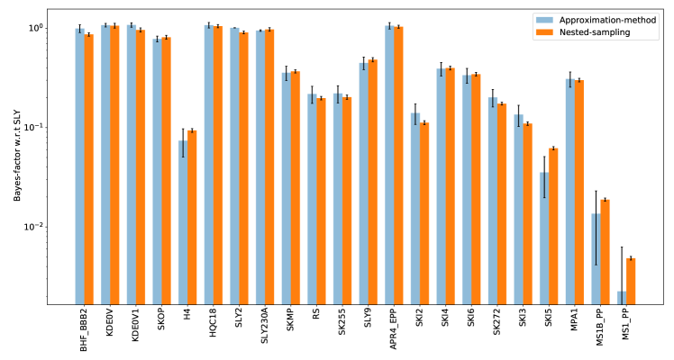
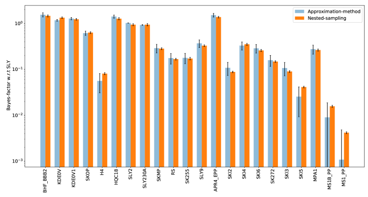
Figure 1: Comparison of Bayes factors obtained with our approximate Bayes factor calculation scheme and the LALInference_nest nested sampling results Abbott et al. (2020a), shown here for the narrow prior in the top panel and the broad prior in the bottom panel. The Bayes factors are computed with respect to the SLY equation of state model in both cases. We show here results for the TaylorF2 waveform. The error-bars for the approximate Bayes factors are an estimate based on standard deviation (see main text). The error-bars in the nested sampling method is obtained from Abbott et al. (2020a).

The results produced from the evidence approximation scheme are generally in good agreement with those produced using the nested sampling method. Note, however, that the Bayes factors obtained within the approximation scheme have large fractional errors for equations of state predicting low evidences. This is due to the intrinsically poor sampling in the regions of parameter space that are least likely a posteriori. The number of samples produced at very large tidal deformabilities is dwarfed by the number of samples produced at more modest tidal deformabilities, because softer equations of state are more preferred by the GW170817 data. This is why we provide the Bayes factors with respect to the SLY equation of state as reference model for which the standard deviation of the evidence computation using the approximation method was relatively small, thus reducing the reference model contribution to the Bayes factor residuals. In Fig. 2 we also show the deviation of the approximation method result with respect to the nested sampling method runs. The deviation is quantified as the absolute value of the difference between the mean value of the Bayes factor calculated by the two methods, divided by the mean value of the Bayes factor calculated by the nested sampling method. In the vertical axis of Fig. 2 we show this deviation as percentage, and find that the deviation is highest for the stiffest equation of state models for both the priors. This is the direct consequence of the sparseness of posterior samples in the region of the parameter space consistent with these equation of state models. The kernel density estimation of the probability density is less reliable at these parts of the parameter space. This is further illustrated in Fig. 3 where we plot the $(\tilde{\Lambda},q)$ posterior distribution for both the priors (narrow and broad) as a scatter plot, along with their KDE as the heat-map. The $(\tilde{\Lambda},q)$ values for some of equation of state models are overlaid on top of the plots. It is immediately evident that the equation of state models which had the highest deviation in Fig. 2 are the ones that are most distant from the peak of the posterior distribution, confirming the aforementioned argument that the KDE is less reliable when number of underlying posteriors samples is very low.

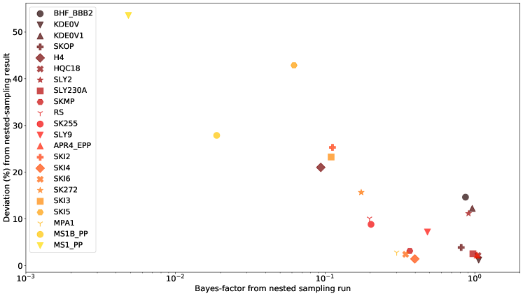
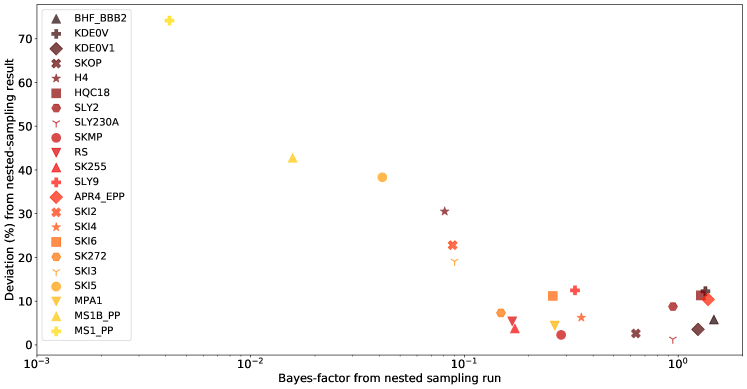
Figure 2: Magnitude of deviation of Bayes factors obtained with our approximate evidence calculation scheme from the LALInference_nest nested sampling results, shown here for the narrow prior in the top panel and the broad prior in the bottom panel. The Bayes factors are again computed with respect to the SLY equation of state model in both cases. We show here results for the TaylorF2 waveform. The deviation is the highest for the stiffest equation of state which has the least evidence in the data. The method is more reliable when the model has good support from the data. The median deviation for the narrow (broad) prior is $10\%(11\%)$.

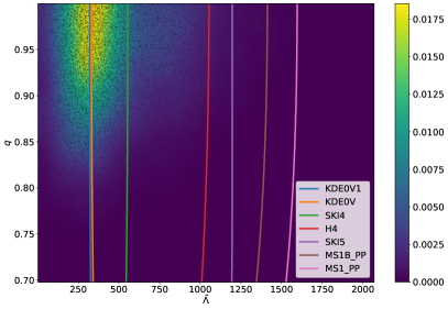
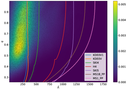
Figure 3: Left: narrow prior: posterior distribution in $(\tilde{\Lambda},q)$ and its KDE. For comparison we show the equation of state curves for various models in $(\tilde{\Lambda},q)$. Note that the models that gave the highest deviation with respect to the nested sampling results in Fig. 2 are also the most distant from the peak of the posterior distribution. Right: broad prior case: we see the identical relationship that for the equation of state models that gave the largest deviation in the Bayes factor computation with respect to the nested sampling results, the posterior support is the weakest. Note that the kinks in the various equation of state models in this plot are due to the fact that it extends to smaller values of $q$, where one of the objects in the binary becomes more massive than the maximum allowed NS mass. At this point we consider that object a black hole and set the value of $\Lambda_{1}=0$. This leads to a sudden change in the value of $\tilde{\Lambda}$ and hence creates these kinks.

An interesting observation can be made from the comparison plot in Fig. 1 top panel. The two equation of state models KDE0V and KDE0V1 are shown to have Bayes factors of $1.075$ and $1.079$ respectively based on the computation using the approximation method. However, the same two equation of state models have Bayes factors of $1.062$ and $0.962$ according to the nested sampling based analysis. As a result of that the Bayes factors computed for KDE0V1 using the two methods seem to be in disagreement. What is surprising is that these two models are very similar as shown in Fig. 3, so one might expect that their Bayes factors as informed by the posterior sample distribution should also be similar. This seems to be the case with the approximation method, while the nested-sampling results are less similar. We think this is happening due to the following reason. For the approximation method, we compute the posterior samples just once. Thus, the KDE obtained for the posterior samples is determined once and for all for each equation of state model. The Bayes factors for KDE0V and KDE0V1 are computed using the same KDE, and since the two models are very similar the Bayes-factor values are also similar.

The resampling technique used to compute the uncertainty captures the fluctuation in the estimation of the KDE due to the finite number of samples. This is what is reported by the error-bars in Fig. 1. However, this technique does not allow us to compute the uncertainty in the Bayes-factor from the posterior samples. In the nested sampling method, however, the Bayes factor is computed for KDE0V and KDE0V1 separately with different nested sampling parameter estimation runs. Thus, the underlying posterior distributions used for computation of the Bayes-factor for these two models are themselves different. The resulting Bayes factor is therefore affected by the inherent variance of the nested sampling runs. The error-bars of the Bayes factors computed from the nested sampling run for the two equation of state overlaps, suggesting that the true Bayes factors of these two models are indeed very close to each other.

Finally, we discuss about the binary black hole model in our approximation scheme. In Ref. Abbott et al. (2020a) the authors have used a binary black hole model as the reference model for the computation of the Bayes factors. One of the shortcomings of the approximation method is that it does not give reliable results for models around part of the parameter space that does not have large posterior support. Moreover, the KDE computation may be less reliable near the boundaries of the parameter space, where posterior sample points consistent with a binary black hole system will be located, leading to large biases in computation of the evidence integral. With this in mind we avoided using binary black hole as a reference equation of state in this work, and have selected the SLY equation of state as the reference, as it was one of the equation of state that has small uncertainty in the value of the evidence integral.

A major advantage of the approximation scheme, shown here to reliably reproduce the evidences calculated in LALInference_nest, is that it allows us to compute the evidence in a fraction of the time taken compared to a full nested sampling run using LALInference_nest. The code to calculate this Ghosh (2020a), as well as demonstrations of how to use the package, are released along with this work in Ghosh (2020b) .

V.2 Stacking of multiple events

Assuming that the equation of state of NS matter is unique, it should be possible to combine information from multiple gravitational wave detections to produce joint inference on the equation of state models. Multiple studies have been conducted to this end to get joint constraints Del Pozzo et al. (2013); Lackey and Wade (2015). In this approximation scheme, multiple detection of gravitational wave events can be incorporated using stacking to make joint inferences on the Bayes-factor between the various models of equation of state. To do so, we simply incorporate this by computing the products of the evidences for the various models.

$$\mathcal{Z}_{E}(d_{1},\ldots,d_{N})=\prod\limits_{i=1}^{N}\mathcal{Z}_{E}(d_{i})\,,$$ (13)

where $\mathcal{Z}_{E}(d_{i})$ is the evidence of the equation of state model ${E}$ for event $i$, and $N$ is the number of detected gravitational wave events. Thus, the joint Bayes factor for $N$ events is given by

$${\rm BF}^{E_{1}}_{E_{2}}({\rm joint})=\frac{\mathcal{Z}_{E_{1}}(d_{1},\ldots,d_{N})}{\mathcal{Z}_{E_{2}}(d_{1},\ldots,d_{N})}\,.$$ (14)

The uncertainty in the joint Bayes factor can be estimated using multiple techniques. In this work we have used the same bootstrapping technique described in Sec. III. For a given pair of equations of state, we resample the Bayes factors for all individual events ten thousand times to obtain a distribution of the joint Bayes factor. The variance of this quantity gives us the estimate of the uncertainty. Following the same procedure we augment the uncertainties of the Bayes factors by a factor of 2 to take into account the effect of oversmoothing of the posterior samples and hence render a conservative estimate.

To test the performance of this stacking method, we conducted a simulation study. We injected the gravitational wave signal of a binary NS system with component masses $(1.4,1.4)\,M_{\odot}$ in simulated Gaussian noise. The tidal deformability of the system was chosen to be consistent with the APR4_EPP equation of state. We injected five gravitational waveforms at 40 Mpc, 70 Mpc, 100 Mpc, 130 Mpc and 160 Mpc respectively. For each event we conducted Bayesian MCMC using LALInference MCMC along with the implementation of the modification of the waveform termination condition discussed earlier. We chose the same broad prior for masses and spins that was described in Sec. III. The result of the study is presented in Fig. 4. We apply a Bayes-factor threshold of $10^{-3}$ in our analysis to exclude some of the stiffest equation of state from the result. This is necessary because for these models the $(q,\tilde{\Lambda})$ posterior samples are poorly sampled by the parameter estimation run, resulting in KDE estimation that is not reliable. The choice of this threshold is motivated by the fact that this was the smallest value of the Bayes-factor for the study using GW170817 (for MS1_PP). This issue can be alleviated by increasing the number of MCMC chains, however for the purpose of demonstration of this method this is unnecessary.

We expected to find that with increasing distance of the injected source the Bayes-factor to converge towards one. When we analyzed the APR4_EPP model itself we found the Bayes-factor with respect to the SLY equation of state to be 1.24, 1.09, 1.07, 1.05, and 1.05 for the above mentioned injected distances respectively. Using the stacking method described above, this led us to a joint Bayes-factor of 1.6 between the APR4_EPP and SLY models. For a disfavored model like SK272 the discrimination ability of the method deteriorates rapidly with lowering of the signal strength. While at 40 Mpc the Bayes-factor for SK272 with respect to SLY is $0.05$, at 70 Mpc, 100 Mpc, 130 Mpc, and 160 Mpc the Bayes-factors are 0.36, 0.58, 0.69, 0.78 respectively, giving a joint Bayes-factor of $5.69\times 10^{-3}$. In Fig. 4 we find that, as expected, the height of the bars are tending towards the asymptotic value of 1.0 as we increase the distance of the source. Note that the heights are more uniform between the different models for the farthest sources. This is due to the fact that weaker signals leave less of an imprint of the tidal deformability in the data to help in discerning between different models. The joint Bayes-factor will be mostly determined by the strongest sources. However, one should also keep in mind the $r^{3}$ distribution of sources. In practice we expect to see more sources at larger distances and fewer sources at closer distances. The combined effect of a large number of weak sources and a small number of strong sources will collectively improve our understanding of the NS equation of state.

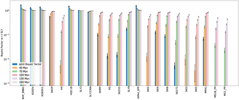
Figure 4: Bayes-factors computed for the various equation of state models for the injected signals at 40 Mpc, 70 Mpc, 100 Mpc, 130 Mpc, and 160 Mpc. The blue bars shows the joint Bayes-factors computed using Eq. 14, which is largely determined by the strongest source. A Bayes-factor threshold of $10^{-3}$ is applied to exclude cases that have very small posterior support.

V.3 Joint Bayes factor from GW170817 and GW190425 using stacking

In Sec. V.2 we introduced the method of stacking in the evidence approximation technique to combine data from multiple BNS coalescence events to get a joint Bayes factor between pairs of equation of state models. In this section we use this method to combine the gravitational-wave data from GW170817 and GW190425, the two BNS coalescences that the LIGO-Virgo interferometers have detected. What makes GW190425 especially interesting is that the heavier object in the binary is estimated to be around $1.60\,M_{\odot}$ to $2.52\,M_{\odot}$ (if we apply a broad prior of the object as mentioned in this work) Abbott et al. (2020b). The upper-limit of the mass of this object is at the edge of maximum NS mass of some equation of state models. Unfortunately, the luminosity distance of this event is $\sim 4$ times greater than the luminosity distance of GW170817. Thus, the strength of the gravitational wave from this event is much weaker across the entire frequency band. This reduction in signal strength, especially in the high frequency regime, severely affects our ability to infer on the tidal deformability and hence the NS equation of state. Thus, we do not expect a very large effect of including the data from GW190425 in the computation of the Bayes factor between the various equation of state models. We conducted Bayesian MCMC parameter estimation run on the data from the interferometers using the specifications detailed in IV. The posterior samples from this run were then used to compute the Bayes factors against the SLY equation of state using the approximation method. We then combine the Bayes factors for the various models with respect to SLY with the same computed for GW170817 using the method of evidence-stacking discussed in Sec. V.2. We show in Fig. 5 the result of this analysis.

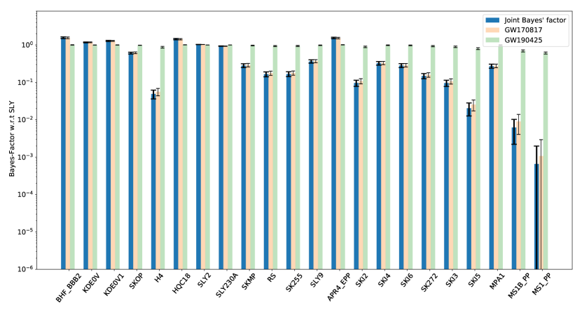
Figure 5: Bayes factor of various equation of state models with respect to SLY model for GW170817, GW190425, and their combination by evidence stacking. Note that the blue bars (joint Bayes factor) and the orange bars (Bayes factor from GW170817 data) are very similar to each other indicating that most of the information in discerning between the different models comes from the data of GW170817. The green bars for GW190425 are adding very little information as can also be seen from the fact that their variation in height across the various models is very small.

EOS	$m_{\max}$	BF(GW170817)	BF(GW190425)	BF(joint)	Fractional change
BHF_BBB2	1.922	1.555	1.006	1.564	0.006
KDE0V	1.96	1.177	0.997	1.174	-0.003
KDE0V1	1.969	1.283	1.001	1.285	0.001
SKOP	1.973	0.618	0.983	0.607	-0.017
H4	2.031	0.056	0.872	0.049	-0.128
HQC18	2.045	1.422	1.009	1.436	0.009
SLY2	2.054	1.028	1.001	1.029	0.001
SLY230A	2.099	0.932	1.003	0.935	0.003
SKMP	2.107	0.29	0.97	0.281	-0.03
RS	2.117	0.176	0.938	0.166	-0.062
SK255	2.144	0.179	0.939	0.168	-0.061
SLY9	2.156	0.37	0.984	0.364	-0.016
APR4_EPP	2.159	1.526	1.012	1.544	0.012
SKI2	2.163	0.108	0.889	0.096	-0.111
SKI4	2.17	0.33	0.983	0.325	-0.017
SKI6	2.19	0.288	0.979	0.282	-0.021
SK272	2.232	0.159	0.933	0.148	-0.067
SKI3	2.24	0.107	0.895	0.096	-0.105
SKI5	2.24	0.025	0.8	0.02	-0.2
MPA1	2.469	0.276	0.987	0.273	-0.013
MS1B_PP	2.747	0.009	0.694	0.006	-0.306
MS1_PP	2.753	0.001	0.611	0.001	-0.389

Table 3: Bayes factors for various equation of state models computed for GW170817, GW190425 and their combined result. The last column shows the fractional change in the Bayes factor for model when evidence GW190425 is stacked with that of GW170817: $[{\rm BF(joint)}-{\rm BF(GW170817)}]/{\rm BF(GW170817)}$. We note a trend that this fractional change in the value of the Bayes factor increases with increasing stiffness of the equation of state model. However, we also notice that there is a direct correlation between the increase in this fractional change with value of the joint Bayes factor.

In Table 3 we present the result of the stacking for all the equation of state models. In this table we show the result of the broad prior only, which is consistently employed for both events. The third column shows the Bayes factor computed using the GW170817 data only, in the fourth column we show the same for GW190425. In the fifth column we show the stacked result. The last column shows the fractional change in the Bayes factor due to the inclusion of the second event, GW190425. This is defined as:

$$\frac{{\rm BF(joint)}-{\rm BF(GW170817)}}{\rm BF(GW170817)}\,.$$ (15)

We find that models which have large Bayes-factor in GW170817 data slightly gain in their Bayes-factor value upon inclusion of the data from GW190425. The gain is around a percent or less. Models that have low Bayes-factors with respect to the SLY equation of state as evidenced from GW170817 data, further diminishes in value upon inclusion of GW190425. This lowering of the Bayes-factor can be substantial for some of the stiffest models like MS1. We notice a slight trend of higher impact of using the second event for stiffer equation of state models (Fig. 6). Note that part of the reason why the Bayes factor changes more for such models could be because of the greater random fluctuation in the individual Bayes factors for them. However, we find that the change is biased toward lower values of the Bayes factors upon stacking the events (hence the negative values in the Fig. 6). If the random fluctuation was the sole reason for this change, this bias should not be present. This provides us an indication, as far as Bayes factor is concerned, that the stiffer models are aggregating more information from GW190425. However, it should also be mentioned that the models for which the addition of GW190425 makes a larger impact are also the ones that have already been found to be highly disfavored by GW170817. In fact the values of joint Bayes-factor are very consistent with the Bayes-factor obtained from GW170817 data, which is in line with the observation made in the injection study in Sec. V.2. Therefore, to gather more insightful results on the equation of state models we will need either stronger signals than GW190425, or a larger number of events.

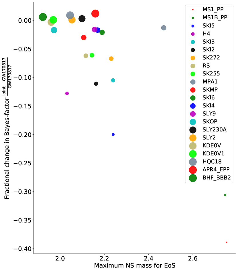
Figure 6: Change in Bayes factor due to inclusion of GW190425 for different equation of state models. The area of the bubbles are proportional to the respective joint Bayes factor values. We note that the models for which the Bayes factor was higher for GW170817 tend to an increased Bayes-factor upon inclusion of the GW190425 data, whereas models which have lower Bayes-factor for GW170817 diminish further upon inclusion of the GW190425 data. However, it should be noted that this effect is very small, given the weakness of the signal from GW190425, as evidenced by the consistency between the bars of Bayes-factors of GW170817 and the joint Bayes-factor in Fig. 5

VI Discussions

The Bayes factor approximation method presented here is designed to help comparisons between a large number of equation of state models for NS matter. The crucial element of this technique is that one only needs a single instance of an equation of state agnostic parameter estimation run conducted with the appropriate priors described above. The approximate Bayes factor between any two arbitrary models can then be computed very rapidly thereafter. The accuracy of the method is reasonably good and continues to perform well even after stacking multiple events as documented in the studies conducted in Secs. V.1 and V.2. We make this method available for public use in the GWXtreme package Ghosh (2020a). Detailed information on using this package is provided in the documentation of the package Ghosh (2020b). The results of this study, including the posterior samples from the parameter estimation analysis that are required for the approximation method are publicly released along with this work Ghosh et al. (2021).

The method can be further extended to estimate parameters describing equation of state models, such as piecewise polytrope or spectral models. To do so, the evidence is interpreted as the marginalized likelihood $\mathcal{L}(d\mid\vec{\Gamma})$ where $\vec{\Gamma}$ are the parameters characterizing the model. One can then impose a prior on these parameters and then the posterior distribution $p(\vec{\Gamma}\mid d)$ can be computed. Evaluating this involves computing the evidence integral in Eq.  12. With $N$ events we simply need to compute $N$ such 1D integrals. This idea is analogous to the method presented in Lackey and Wade (2015), where the evidence integral is carried out in $(m_{1},m_{2},\tilde{\Lambda})$ space. Under this approximation scheme we compute a 1D line integral instead. This will provide a joint posterior distribution of the piecewise polytrope parameters or the spectral parameters.

There are however three caveats that we would like the users of the package to be aware of. First, this method employs kernel density estimation to conduct the integration for the computation of the Bayes factor. The KDE over-smooths the underlying distribution of the sample, and as a result biases the estimation of the uncertainty. The uncertainty measurement technique used in this work is not capable of quantitatively taking into consideration of this effect, and as a result we only provide an approximate error estimate. In future work we will provide a more quantitative handle on the uncertainty. Second, in the case of GW170817 the lack of samples at low tidal deformability results in Bayes factor computation with large statistical fluctuations when extremely soft models are used as the reference equation of state. It is generally safe to use a reference equation of state that has good overlap with the posterior distribution (hence the choice of SLY in this work). We encourage the use of SLY (or similar) equation of state as the reference model for the computation of Bayes factor for any equation of state that has not been covered in this analysis. Finally, the choice of the uniform priors in $\tilde{\Lambda}$ and $\delta\tilde{\Lambda}$ results in some negative values in tidal deformabilities of the individual stars. This will be a problem for any waveform generator that requires the individual tidal deformabilities to be positive. In this work we chose to use the TaylorF2 waveform since only $\tilde{\Lambda}$ is required to generate the waveform. For other waveforms we will have to switch back to a uniform prior in individual tidal deformabilities. However, at that point samples would need to be reweighted such that the approximation in Eq. (11) works. This will be included in future release of the GWXtreme.

Appendix: ESTIMATION OF UNCERTAINTY SCALING-FACTOR

The KDE resampling method for estimating the uncertainty discussed in Sec. III cannot account for potential systematic bias inherent in the KDE approximation. We account for this by applying a correction factor of 2 to the estimated standard deviation. In the following we explain how this factor is chosen.

First, we set up a probability density function (PDF) $p_{\mathrm{ex}}(q,\tilde{\Lambda})$ that is intended to be an example of the PDF used in Eq. 11, representative for events our method might be applied to. One option would be to use the KDE obtained from our GW170817 posterior sample distribution as PDF. However, the sharpness of features would be limited by the KDE bandwidth. In our approximation method we employ Scott’s bandwidth given by $N^{-1/6}$, where $N$ is the number of posterior samples. To obtain an example PDF with somewhat sharper features, we duplicate each posterior sample and then create the KDE.

Since the example posterior is provided as a PDF instead of a sample distribution, the corresponding evidence for a given equation of state can be computed exactly. We compute the exact Bayes factors with respect to the SLY model, $B_{e}$, for a representative subset of equations of state, consisting of APR4_EPP, H4, KDE0V, SKI2, SKI5, MS1B_PP, and MS1_PP, covering a wide range of stiffness.

To simulate a posterior sample distribution as obtained from a parameter estimation run, we draw the same number of samples from $p_{\mathrm{ex}}$ as contained in our real posterior sample distribution for GW170817. We do this repeatedly, creating 500 example posterior sample distributions. To each of those sample distributions, we apply the evidence approximation method. We thus obtain 500 samples for the estimated Bayes factor, $B_{e}^{s}$, and for the estimated standard deviation, $\sigma_{e}^{s}$ (not including the correction factor).

For each equation of state, we compute the distribution for $C_{e}=(B_{e}^{s}-B_{e})/\bar{\sigma}_{e}$, i.e. the true error of the approximated Bayes factor normalized to the mean $\bar{\sigma}_{e}$ of the error estimate $\sigma_{e}^{s}$. We further combine the sample distributions $C_{e}$ for the different equations of state into a single distribution $C$, using equal weights. This distribution is roughly Gaussian and centered around zero. The one-sigma interval is $|C|<1.24$, and in 89.3% of the cases $|C|<2$. Hence, our chosen correction factor of 2 is larger than required for the example tested here. This is an added precaution owed to the ad hoc choice of the test case.

References

- Oppenheimer and Volkoff (1939) J. R. Oppenheimer and G. M. Volkoff, Phys. Rev. 55, 374 (1939).
- Özel and Freire (2016) F. Özel and P. Freire, Annual Review of Astronomy and Astrophysics 54, 401 (2016), https://doi.org/10.1146/annurev-astro-081915-023322 .
- Lindblom (1992) L. Lindblom, The Astrophysical Journal 398, 569 (1992).
- Manchester et al. (2005) R. N. Manchester, G. B. Hobbs, A. Teoh, and M. Hobbs, The Astronomical Journal 129, 1993 (2005).
- ATNF-CSIRO (2019) ATNF-CSIRO, “ATNF Pulsar Catalog,” https://www.atnf.csiro.au/research/pulsar/psrcat/ (2019), [Online; accessed 19-Nov-2019].
- NASA (2019) NASA, “NICER,” https://www.nasa.gov/nicer (2019), [Online; accessed 26-Nov-2019].
- Miller et al. (2019) M. C. Miller et al., Astrophys. J. Lett. 887, L24 (2019), arXiv:1912.05705 [astro-ph.HE] .
- Riley et al. (2019) T. E. Riley, A. L. Watts, S. Bogdanov, P. S. Ray, R. M. Ludlam, S. Guillot, Z. Arzoumanian, C. L. Baker, A. V. Bilous, D. Chakrabarty, K. C. Gendreau, A. K. Harding, W. C. G. Ho, J. M. Lattimer, S. M. Morsink, and T. E. Strohmayer, The Astrophysical Journal 887, L21 (2019).
- Aasi et al. (2015) J. Aasi et al. (LIGO Scientific), Class. Quant. Grav. 32, 074001 (2015), arXiv:1411.4547 [gr-qc] .
- Acernese et al. (2015) F. Acernese et al. (VIRGO), Class. Quant. Grav. 32, 024001 (2015), arXiv:1408.3978 [gr-qc] .
- Poisson (1998) E. Poisson, Phys. Rev. D 57, 5287 (1998).
- Hinderer (2008) T. Hinderer, The Astrophysical Journal 677, 1216 (2008).
- Flanagan and Hinderer (2008) E. E. Flanagan and T. Hinderer, Phys. Rev. D77, 021502 (2008), arXiv:0709.1915 [astro-ph] .
- Read et al. (2009a) J. S. Read, C. Markakis, M. Shibata, K. Uryu, J. D. E. Creighton, and J. L. Friedman, Phys. Rev. D79, 124033 (2009a), arXiv:0901.3258 [gr-qc] .
- Del Pozzo et al. (2013) W. Del Pozzo, T. G. F. Li, M. Agathos, C. Van Den Broeck, and S. Vitale, Phys. Rev. Lett. 111, 071101 (2013), arXiv:1307.8338 [gr-qc] .
- Agathos et al. (2015) M. Agathos, J. Meidam, W. Del Pozzo, T. G. F. Li, M. Tompitak, J. Veitch, S. Vitale, and C. Van Den Broeck, Phys. Rev. D92, 023012 (2015), arXiv:1503.05405 [gr-qc] .
- van der Sluys et al. (2009) M. van der Sluys, I. Mandel, V. Raymond, V. Kalogera, C. Röver, and N. Christensen, Classical and Quantum Gravity 26, 204010 (2009).
- Veitch and Vecchio (2010) J. Veitch and A. Vecchio, Phys. Rev. D 81, 062003 (2010).
- Raymond et al. (2010) V. Raymond, M. V. van der Sluys, I. Mandel, V. Kalogera, C. Röver, and N. Christensen, Classical and Quantum Gravity 27, 114009 (2010).
- Rodriguez et al. (2014) C. L. Rodriguez, B. Farr, V. Raymond, W. M. Farr, T. B. Littenberg, D. Fazi, and V. Kalogera, The Astrophysical Journal 784, 119 (2014).
- Veitch et al. (2015) J. Veitch et al., Phys. Rev. D 91, 042003 (2015).
- Abbott et al. (2019) B. P. Abbott et al. (LIGO Scientific Collaboration and Virgo Collaboration), Phys. Rev. X 9, 011001 (2019).
- Abbott et al. (2018) B. P. Abbott et al. (The LIGO Scientific Collaboration and the Virgo Collaboration), Phys. Rev. Lett. 121, 161101 (2018).
- De et al. (2018) S. De, D. Finstad, J. M. Lattimer, D. A. Brown, E. Berger, and C. M. Biwer, Phys. Rev. Lett. 121, 091102 (2018).
- Read et al. (2009b) J. S. Read, B. D. Lackey, B. J. Owen, and J. L. Friedman, Phys. Rev. D 79, 124032 (2009b).
- Lindblom (2010) L. Lindblom, Phys. Rev. D 82, 103011 (2010).
- Landry and Essick (2019) P. Landry and R. Essick, Phys. Rev. D 99, 084049 (2019), arXiv:1811.12529 [gr-qc] .
- Landry et al. (2020) P. Landry, R. Essick, and K. Chatziioannou, Phys. Rev. D 101, 123007 (2020), arXiv:2003.04880 [astro-ph.HE] .
- Capano et al. (2020) C. D. Capano, I. Tews, S. M. Brown, B. Margalit, S. De, S. Kumar, D. A. Brown, B. Krishnan, and S. Reddy, Nature Astron. 4, 625 (2020), arXiv:1908.10352 [astro-ph.HE] .
- Dietrich et al. (2020) T. Dietrich, M. W. Coughlin, P. T. H. Pang, M. Bulla, J. Heinzel, L. Issa, I. Tews, and S. Antier, Science 370, 1450 (2020), https://science.sciencemag.org/content/370/6523/1450.full.pdf .
- Abbott et al. (2020a) B. P. Abbott et al. (LIGO Scientific, Virgo), Class. Quant. Grav. 37, 045006 (2020a), arXiv:1908.01012 [gr-qc] .
- Abbott et al. (2021) B. P. Abbott et al., SoftwareX 13, 100658 (2021).
- LIGO Scientific Collaboration, Virgo Collaboration (2017) LIGO Scientific Collaboration, Virgo Collaboration, “GW170817,” https://www.gw-openscience.org/eventapi/html/GWTC-1-confident/GW170817/v3 (2017).
- Skilling (2004) J. Skilling, in Bayesian Inference and Maximum Entropy Methods in Science and Engineering: 24th International Workshop on Bayesian Inference and Maximum Entropy Methods in Science and Engineering, American Institute of Physics Conference Series, Vol. 735, edited by R. Fischer, R. Preuss, and U. V. Toussaint (2004) pp. 395–405.
- Favata (2014) M. Favata, Phys. Rev. Lett. 112, 101101 (2014), arXiv:1310.8288 [gr-qc] .
- Wade et al. (2014) L. Wade, J. D. E. Creighton, E. Ochsner, B. D. Lackey, B. F. Farr, T. B. Littenberg, and V. Raymond, Phys. Rev. D89, 103012 (2014), arXiv:1402.5156 [gr-qc] .
- Bini et al. (2012) D. Bini, T. Damour, and G. Faye, Phys. Rev. D 85, 124034 (2012), arXiv:1202.3565 [gr-qc] .
- LIGO Scientific Collaboration, Virgo Collaboration (2018) LIGO Scientific Collaboration, Virgo Collaboration, “LALSuite,” https://git.ligo.org/lscsoft/lalsuite (2018).
- Metropolis et al. (1953) N. Metropolis et al., J. Chem. Phys. 21, 1087 (1953).
- Hastings (1970) W. Hastings, Biometrika 57, 97 (1970).
- Abbott et al. (2020b) B. P. Abbott et al. (LIGO Scientific, Virgo), Astrophys. J. Lett. 892, L3 (2020b), arXiv:2001.01761 [astro-ph.HE] .
- LIGO Scientific Collaboration, Virgo Collaboration (2019) LIGO Scientific Collaboration, Virgo Collaboration, “GW190425,” https://www.gw-openscience.org/eventapi/html/O3_Discovery_Papers/GW190425/v1 (2019).
- Ghosh (2020a) S. Ghosh, “GWXtreme package,” https://pypi.org/project/GWXtreme/ (2020a), [Online; accessed 07-Jun-2020].
- Ghosh (2020b) S. Ghosh, “GWXtreme documentation,” https://gwxtreme.readthedocs.io/en/latest/ (2020b), [Online; accessed 07-Jun-2020].
- Lackey and Wade (2015) B. D. Lackey and L. Wade, Phys. Rev. D 91, 043002 (2015), arXiv:1410.8866 [gr-qc] .
- Ghosh et al. (2021) S. Ghosh, X. Liu, J. Creighton, W. Kastaun, G. Pratten, and I. Magaña, “Dataset for rapid model comparison of equations of state from gravitational wave observation of binary neutron star coalescences,” (2021).