Improving Question Answering Model Robustness with
Synthetic Adversarial Data Generation

Abstract

Despite recent progress, state-of-the-art question answering models remain vulnerable to a variety of adversarial attacks. While dynamic adversarial data collection, in which a human annotator tries to write examples that fool a model-in-the-loop, can improve model robustness, this process is expensive which limits the scale of the collected data. In this work, we are the first to use synthetic adversarial data generation to make question answering models more robust to human adversaries. We develop a data generation pipeline that selects source passages, identifies candidate answers, generates questions, then finally filters or re-labels them to improve quality. Using this approach, we amplify a smaller human-written adversarial dataset to a much larger set of synthetic question-answer pairs. By incorporating our synthetic data, we improve the state-of-the-art on the AdversarialQA dataset by 3.7F${}_{\text{1}}$ and improve model generalisation on nine of the twelve MRQA datasets. We further conduct a novel human-in-the-loop evaluation and show that our models are considerably more robust to new human-written adversarial examples: crowdworkers can fool our model only $8.8\%$ of the time on average, compared to $17.6\%$ for a model trained without synthetic data.

1 Introduction

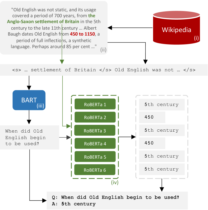
Figure 1: The Synthetic Adversarial Data Generation Pipeline showing: (i) passage selection from Wikipedia; (ii) answer candidate selection and filtering by model confidence (an example retained answer shown in green, and a dropped answer candidate in red); (iii) question generation using BART${}_{\text{Large}}$; and (iv) answer re-labelling using self-training. The generated synthetic data is then used as part of the training data for a downstream Reading Comprehension model.

Large-scale labelled datasets like SQuAD Rajpurkar et al. (2016) and SNLI Bowman et al. (2015) have been driving forces in natural language processing research. Over the past few years, however, such “statically collected” datasets have been shown to suffer from various problems. In particular, they often exhibit inadvertent spurious statistical patterns that models learn to exploit, leading to poor model robustness and generalisation Jia and Liang (2017); Gururangan et al. (2018); Geva et al. (2019); McCoy et al. (2019); Lewis et al. (2021a).

A recently proposed alternative is dynamic data collection Bartolo et al. (2020); Nie et al. (2020), where data is collected with both humans and models in the annotation loop. Usually, these humans are instructed to ask adversarial questions that fool existing models. Dynamic adversarial data collection is often used to evaluate the capabilities of current state-of-the-art models, but it can also create higher-quality training data Bartolo et al. (2020); Nie et al. (2020) due to the added incentive for crowdworkers to provide challenging examples. It can also reduce the prevalence of dataset biases and annotator artefacts over time Bartolo et al. (2020); Nie et al. (2020), since such phenomena can be subverted by model-fooling examples collected in subsequent rounds. However, dynamic data collection can be more expensive than its static predecessor as creating examples that elicit a certain model response (i.e., fooling the model) requires more annotator effort, resulting in more time spent, and therefore higher cost per example.

In this work, we develop a synthetic adversarial data generation pipeline, making novel contributions to the answer selection, question generation, and filtering and re-labelling tasks. We show that dynamic adversarial data collection can be made more sample efficient by synthetically generating (see Figure 1) examples that improve the robustness of models in terms of performance on adversarially-collected datasets, comprehension skills, and domain generalisation.

We are also the first to evaluate models in-the-loop for robustness to human adversaries using the macro-averaged validated model error rate, demonstrating considerable improvements with crowdworkers only able to fool the model-in-the-loop 8.8% of the time on average, compared to 17.6% for our best baseline. The collected dataset will form part of the evaluation for a new round of the Dynabench QA task.

2 Related Work

2.1 Adversarial Data Collection

We directly extend the AdversarialQA dataset collected in “Beat the AI” (Bartolo et al., 2020), which uses the same passages as SQuAD1.1. AdversarialQA was collected by asking crowdworkers to write extractive question-answering examples that three different models-in-the-loop were unable to answer correctly, creating the $\mathcal{D_{\mathrm{BiDAF}}}$, $\mathcal{D_{\mathrm{BERT}}}$, and $\mathcal{D_{\mathrm{RoBERTa}}}$ subsets.

Other datasets for question answering (Rajpurkar et al., 2018; Dua et al., 2019; Wallace et al., 2019), sentiment analysis (Potts et al., 2021), hate speech detection (Vidgen et al., 2021), and natural language inference (Nie et al., 2020) have been collected in a similar manner. While appealing, human-generated adversarial data is expensive to collect; our work is complementary in that it explores methods to extract further value from existing adversarially collected datasets without requiring additional annotation effort.

2.2 Synthetic Question Generation

Many approaches have been proposed to generate question-answer pairs given a passage (Du et al., 2017; Du and Cardie, 2018; Zhao et al., 2018; Lewis and Fan, 2019; Alberti et al., 2019; Puri et al., 2020; Lewis et al., 2021b). These generally use a two-stage pipeline that first identifies an answer conditioned on a passage, then generates a question conditioned on the passage and answer; we train a similar pipeline in our work.

G-DAUG (Yang et al., 2020) trains generative models to synthesise training data for commonsense reasoning. Our work focuses on extractive question-answering (QA), which motivates the need for different generative models. Yang et al. (2020) filter generated examples using influence functions, or methods that attempt to maximise diversity; we find that a different approach that considers answer agreement between QA models trained with different random seeds leads to better performance in our setting.

2.3 Self-training

In self-training, a model is trained to both predict correctly on labelled examples and increase its confidence on unlabelled examples. Self-training can yield complementary accuracy gains with pretraining (Du et al., 2020) and can improve robustness to domain shift (Kumar et al., 2020). In our setting, large amounts of unlabelled adversarial-style questions are not readily available, which motivates our use of a question generation model.

2.4 Human Evaluation

The ultimate goal of automatic machine learning model evaluation is usually stated as capturing human judgements Callison-Burch et al. (2006); Hill et al. (2015); Vedantam et al. (2015); Liu et al. (2016). Evaluation with real humans is considered beneficial, but not easily scalable, and as such is rarely conducted in-the-loop. With NLP model capabilities ever improving, adversarial worst case evaluation becomes even more pertinent. To our knowledge, this work is the first to compare models explicitly by their adversarial validated model error rate (vMER), which we define in Section 4.4.

3 Synthetic Data Generation

We develop a synthetic data generation pipeline for QA that involves four stages: passage selection, answer candidate selection, question generation, and synthetic data filtering and re-labelling. Due to the complexity of the system, we study each of these in isolation, and then combine our best identified approaches for the final systems. We evaluate each component both intrinsically and on their contribution to downstream QA performance on the AdversarialQA test sets and an unseen split of the SQuAD1.1 dev set. The final synthetic data generation pipeline consists of:

1. Passage selection: we use passages from Wikipedia for this work.

2. Answer Candidate selection: the model identifies spans within the passage that are likely to be answers to a question.

3. Question Generation: a generative model is used to generate a question, conditioned on the passage and each answer.

4. Filtering and Re-labelling: synthetic question-answer pairs that do not meet the necessary criteria are discarded, or have their answers re-labelled using self-training.

Results for the baseline and overall best performing systems are shown in Table 7. Results for ELECTRA_Large (Clark et al., 2020) showing further performance gains are in Appendix J.

3.1 Data Generation Pipeline

Model	Precision (%)	Recall (%)	F${}_{\text{1}}$ (%)
POS Extended	12.7	65.2	20.7
Noun Chunks	17.4	36.9	22.5
Named Entities	30.3	30.0	27.1
Span Extraction, k=15	22.5	26.6	23.7
BART${}_{\text{ans. only}}$, k=15	27.7	31.3	28.6
SAL (ours)	28.6	44.2	33.7

Table 1: Answer selection results on aligned test set.

Method	#QA pairs	$\mathcal{D_{\mathrm{SQuAD}}}$		$\mathcal{D_{\mathrm{BiDAF}}}$		$\mathcal{D_{\mathrm{BERT}}}$		$\mathcal{D_{\mathrm{RoBERTa}}}$
		EM	F${}_{\text{1}}$	EM	F${}_{\text{1}}$	EM	F${}_{\text{1}}$	EM	F${}_{\text{1}}$
POS Extended	999,034	53.8	71.4	32.7	46.9	30.8	40.2	20.4	27.9
Noun Chunks	581,512	43.3	63.7	28.7	43.1	22.3	31.4	18.2	27.4
Named Entities	257,857	54.2	69.7	30.5	42.5	26.6	35.4	18.1	24.0
Span Extraction	377,774	64.7	80.1	37.8	53.9	27.7	39.1	16.7	26.9
SAL (ours)	566,730	68.2	82.6	43.2	59.3	34.9	45.4	25.2	32.8
SAL threshold (ours)	393,164	68.5	82.0	46.0	60.3	36.5	46.8	24.2	32.4

Table 2: Downstream test results for a RoBERTa${}_{\text{Large}}$ QA model trained on synthetic data generated using different answer selection methods combined with a BART${}_{\text{Large}}$ question generator (trained on SQuAD_10k + $\mathcal{D_{\mathrm{AQA}}}$).

In order to generate synthetic adversarial examples, we first select passages, then identify candidate answers in those passages, generate corresponding questions for these answers, and then filter or re-label for improved quality based on various criteria.

3.1.1 Passage Selection

The text passages we use are sourced from SQuAD (further details can be found in Appendix A). We also experiment with using passages external to SQuAD, which are also sourced from Wikipedia. To preserve evaluation integrity, we analyse the 8-gram overlap of all external passages to the evaluation datasets, after normalisation to lower-cased alphanumeric words with a single space delimiter Radford et al. (2019). We find that just 0.3% of the external passages have any overlap with the evaluation sets, and filter these out.

3.1.2 Answer Candidate Selection

The next step is to identify which spans of text within the passages are likely to be answers to a question. We investigate a range of existing methods for answer candidate selection, which takes the passage as input and outputs a set of possible answers. We further propose a self-attention-based classification head that jointly models span starts and ends, with improved performance.

Since SQuAD and the AdversarialQA datasets use the same passages partitioned into the same data splits, we align the annotated answers to create representative answer selection training, validation and test sets. Dataset statistics (see Appendix C), highlight the high percentage of overlapping answers suggesting that existing answer tagging methods Zhou et al. (2017); Zhao et al. (2018) might struggle, and models should ideally be capable of handling span overlap.

Baseline Systems

We investigate three baseline systems; noun phrases and named entities following Lewis et al. (2019), as well as an extended part-of-speech tagger incorporating named entities, adjectives, noun phrases, numbers, distinct proper nouns, and clauses.

Span Extraction

We fine-tune a RoBERTa${}_{\text{Large}}$ span extraction model as investigated in previous work Alberti et al. (2019); Lewis and Fan (2019). We treat the number of candidates to sample as a hyper-parameter and select the optimal value for $k\in\{1,5,10,15,20\}$ on the validation set.

Generative Answer Detection

We use BART${}_{\text{Large}}$ Lewis et al. (2020) in two settings; one generating answer and question, and the other where we generate the answer only, as we find that this setting provides better control of answer diversity. We use the same range of $k\in\{1,5,10,15,20\}$ for both settings.

Self-Attention Labelling (SAL)

We propose a multi-label classification head to jointly model candidate start and end tokens, and provide a binary label for whether each possible span of text from the passage is a candidate answer. We adapt scaled dot-product attention Vaswani et al. (2017) where the candidate start, S, and end, E, token representations are analogous to the projected layer input queries and keys. We apply a sigmoid over the computed attention scores, giving a matrix where each cell gives the probability $p(a_{ij}|c)$ of whether the span in the context, $c$, with start index $i$ and end index $j$ is a valid answer candidate. Formally:

$$p(a_{ij}|c)=\sigma\left(\frac{\sum_{k=1}^{d}s_{ik}e_{kj}}{\sqrt{d}}\right)$$

We optimise using binary cross-entropy, masking out impossible answer spans defined as those not in the passage, with end indices before start, or longer than the maximum permitted answer length, and upweigh positive examples to help counteract the class imbalance. We decode from the output probability matrix to the original passage tokens using a reversible tokeniser and use a probability threshold of $0.5$ for candidate selection, which can be adapted to tune precision and recall.

While answer candidate selection only requires a single attention head, the multi-head implementation allows application to any labelling task requiring span modelling with overlaps, where each head is trained to predict labels for each class, such as for nested Named Entity Recognition. We implement this in Transformers Wolf et al. (2020) and fine-tune RoBERTa${}_{\text{Large}}$ with SAL on the answer selection dataset.

Evaluation

We evaluate performance on the answer selection dataset using entity-level precision, recall, and F${}_{\text{1}}$ on unique normalised candidates. Results are shown in Table 1. We further investigate the effects of different answer candidate selection methods on downstream QA model performance (see Table 2) by training a RoBERTa${}_{\text{Large}}$ model on synthetic QA pairs generated when using different answer selection methods. To eliminate generated dataset size as a potential confounder, we also replicate these experiments using a sample of 87,000 examples and find similar results (see Appendix C).

3.1.3 Question Generation

Once answer candidates have been identified for a selected passage, we then generate a corresponding question by directly fine-tuning a BART${}_{\text{Large}}$ (Lewis et al., 2020) autoregressive sequence generation decoder. To discourage the model from memorising the questions in the SQuAD training set and directly reproducing these, we train on a subset of 10k examples from SQuAD, selected such that they correspond to the same source passages as the AdversarialQA training data. This ensures that when scaling up synthetic generation, the vast majority of passages are previously completely unseen to the generator.

Context: Following the series revival in 2005, Derek Jacobi ANS provided the character’s re-introduction in the 2007 episode "Utopia". During that story the role was then assumed by John Simm who returned to the role multiple times through the Tenth Doctor’s tenure. As of the 2014 episode "Dark Water," it was revealed that the Master had become a female incarnation or "Time Lady," going by the name of "Missy", played by Michelle Gomez.
SQuAD10k	Who portrayed the Master in the 2007 episode "Utopia"?
$\mathcal{D_{\mathrm{BiDAF}}}$	Who replaced John Simm as the Tenth Doctor? (Answer Mismatch)
$\mathcal{D_{\mathrm{BERT}}}$	Who played the Master in the 2007 episode "Utopia"?
$\mathcal{D_{\mathrm{RoBERTa}}}$	Who was the first actor to play the Master?
$\mathcal{D_{\mathrm{AQA}}}$	Who played the Master first, Derek Jacobi or John Simm?
SQuAD10k + $\mathcal{D_{\mathrm{AQA}}}$	Who re-introduced the character of the Master?

Table 3: Examples of questions generated using BART trained on different source datasets.

Model	Valid	Answer Mismatch	Ungramm-atical	Invalid
SQuAD10k	90.0%	10.0%	0.0%	0.0%
$\mathcal{D_{\mathrm{BiDAF}}}$	70.0%	30.0%	0.0%	0.0%
$\mathcal{D_{\mathrm{BERT}}}$	76.7%	23.3%	0.0%	0.0%
$\mathcal{D_{\mathrm{RoBERTa}}}$	70.0%	20.0%	0.0%	10.0%
$\mathcal{D_{\mathrm{AQA}}}$	76.7%	16.7%	0.0%	6.7%
SQuAD10k+$\mathcal{D_{\mathrm{AQA}}}$	93.3%	6.7%	0.0%	0.0%

Table 4: Manual analysis of questions generated when training on different source data.

Source Questions

Since the types of questions a generative model is trained on can impact both performance and diversity, we experiment with training on SQuAD and different subsets of AdversarialQA, and the combination of both. Examples of the generated questions are shown in Table 3.

We carry out a manual answerability analysis on a random sample of 30 generated questions (using beam search with $k=5$) in each of these settings (see Table 4 and Appendix B). We define answerability by the following criteria: (i) The question must be answerable from a single continuous span in the passage; (ii) There must be only one valid (or clearly one most valid) answer (e.g. in the case of a co-reference the canonical entity name should be the answer); (iii) A human should be able to answer the question correctly given sufficient time; and (iv) The correct answer is the one on which the model was conditioned during question generation. We find that when the models attempt to generate complex questions, the generated question is often inconsistent with the target answer, despite remaining well-formed. We also observe that when the generated question requires external knowledge (e.g. “What is a tribe?” or “Which is not a country?”) the models are reasonably consistent with the answer, however, they often lose answer consistency when answering the question requires resolving information in the passage (e.g. “What is the first place mentioned?”).

Method	#QA pairs	$\mathcal{D_{\mathrm{SQuAD}}}$		$\mathcal{D_{\mathrm{BiDAF}}}$		$\mathcal{D_{\mathrm{BERT}}}$		$\mathcal{D_{\mathrm{RoBERTa}}}$
		EM	F${}_{\text{1}}$	EM	F${}_{\text{1}}$	EM	F${}_{\text{1}}$	EM	F${}_{\text{1}}$
R${}_{\text{SQuAD}}$	87,599	73.2	86.3	48.9	64.3	31.3	43.5	16.1	26.7
R${}_{\text{SQuAD+AQA}}$	117,599	74.2	86.9	57.4	72.2	53.9	65.3	43.4	54.2
SQuAD10k	87,598	69.2	82.6	37.1	52.1	22.4	32.3	13.9	22.3
$\mathcal{D_{\mathrm{BiDAF}}}$	87,598	67.1	80.4	41.4	56.5	33.1	43.8	22.0	32.5
$\mathcal{D_{\mathrm{BERT}}}$	87,598	67.4	80.2	36.3	51.1	30.3	40.6	18.8	29.5
$\mathcal{D_{\mathrm{RoBERTa}}}$	87,598	63.4	77.9	32.6	47.9	27.2	37.5	20.6	32.0
$\mathcal{D_{\mathrm{AQA}}}$	87,598	65.5	80.1	37.0	53.0	31.1	40.9	23.2	33.3
SQuAD10k + $\mathcal{D_{\mathrm{AQA}}}$	87,598	71.9	84.7	44.1	58.8	32.9	44.1	19.1	28.8

Table 5: Downstream QA test results using generative models trained on different source data. We compare these results to baseline RoBERTa models trained on SQuAD, and on the combination of SQuAD and AdversarialQA.

For each of these models, we generate 87k examples (the same size as the SQuAD training set to facilitate comparison) using the human-provided answers, and then measure the effects on downstream performance by training a QA model on this synthetic data. Results are shown in Table 5. We find that, in this setting, the best source data for the generative model is consistently the combination of SQuAD and AdversarialQA. We also note that using only synthetic generated data, we can achieve good performance on $\mathcal{D_{\mathrm{SQuAD}}}$ consistent with the findings of Puri et al. (2020), and outperform the model trained on the human-written SQuAD data on $\mathcal{D_{\mathrm{BERT}}}$ (+0.6F${}_{\text{1}}$) and $\mathcal{D_{\mathrm{RoBERTa}}}$ (+6.6F${}_{\text{1}}$). This is in line with the observations of Bartolo et al. (2020) suggesting that the distribution of the questions collected using progressively stronger models-in-the-loop is less similar to that of SQuAD. It also shows that the generator can successfully identify and reproduce patterns of adversarially-written questions. However, the results using synthetic data alone are considerably worse than when training the QA model on human-written adversarial data with, for example, a performance drop of 21.2F${}_{\text{1}}$ for $\mathcal{D_{\mathrm{BERT}}}$. This suggests that while we can do well on SQuAD using synthetic questions alone, we may need to combine the synthetic data with the human-written data for best performance in the more challenging adversarial settings.

Question Diversity

In order to provide training signal diversity to the downstream QA model, we experiment with a range of decoding techniques (see Appendix D), and then evaluate these by downstream performance of a QA model trained on the questions generated in each setting. We observe minimal variation in downstream performance as a result of question decoding strategy, with the best downstream results obtained using nucleus sampling ($top_{p}=0.75$). However, we also obtain similar downstream results with standard beam search using a beam size of 5. We find that, given the same computational resources, standard beam search is roughly twice as efficient, and therefore opt for this approach for our following experiments.

3.1.4 Filtering and Re-labelling

Filtering Method	#QA pairs	$\mathcal{D_{\mathrm{SQuAD}}}$		$\mathcal{D_{\mathrm{BiDAF}}}$		$\mathcal{D_{\mathrm{BERT}}}$		$\mathcal{D_{\mathrm{RoBERTa}}}$
		EM	F${}_{\text{1}}$	EM	F${}_{\text{1}}$	EM	F${}_{\text{1}}$	EM	F${}_{\text{1}}$
Answer Candidate Conf. ($thresh=0.6$)	362,281	68.4	82.4	42.9	57.9	36.3	45.9	28.0	36.5
Question Generator Conf. ($thresh=0.3$)	566,725	69.3	83.1	43.5	58.9	36.3	46.6	26.2	34.8
Influence Functions	288,636	68.1	81.9	43.7	58.6	36.1	46.6	27.4	36.4
Ensemble Roundtrip Consistency ($6/6$ correct)	250,188	74.2	86.2	55.1	67.7	45.8	54.6	31.9	40.3
Self-training (ST)	528,694	74.8	87.0	53.9	67.9	47.5	57.6	35.2	44.6
Answer Candidate Conf. ($thresh=0.5$) & ST	380,785	75.1	87.0	56.5	70.0	47.9	58.7	36.0	45.9

Table 6: Downstream QA test results for different filtering strategies, showing best hyper-parameter settings.

The synthetic question generation process can introduce various sources of noise, as seen in the previous analysis, which could negatively impact downstream results. To mitigate these effects, we explore a range of filtering and re-labelling methods. Results for the best performing hyper-parameters of each method are shown in Table 6 and results controlling for dataset size are in Appendix E.

Answer Candidate Confidence

We select candidate answers using SAL (see section 3.1.2), and filter based on the span extraction confidence of the answer candidate selection model.

Question Generator Confidence

We filter out samples below various thresholds of the probability score assigned to the generated question by the question generation model.

Influence Functions

We use influence functions (Cook and Weisberg, 1982; Koh and Liang, 2017) to estimate the effect on the validation loss of including a synthetic example as explored by Yang et al. (2020), but adapted for QA. We filter out examples estimated to increase the validation loss.

Ensemble Roundtrip Consistency

Roundtrip consistency (Alberti et al., 2019; Fang et al., 2021) uses an existing fine-tuned QA model to attempt to answer the generated questions, ensuring that the predicted answer is consistent with the target answer prompted to the generator. Since our setup is designed to generate questions which are intentionally challenging for the QA model to answer, we attempt to exploit the observed variation in model behaviour over multiple random seeds, and replace the single QA model with a six-model ensemble. We find that filtering based on the number of downstream models that correctly predict the original target answer for the generated question produces substantially better results than relying on the model confidence scores, which could be prone to calibration imbalances across models.

Self-training

Filtering out examples that are not roundtrip-consistent can help eliminate noisy data, however, it also results in (potentially difficult to answer) questions to which a valid answer may still exist being unnecessarily discarded. Self-training has been shown to improve robustness to domain shift (Kumar et al., 2020) and, in our case, we re-label answers to the generated questions based on the six QA model predictions.

Specifically, in our best-performing setting, we keep any examples where at least five of the six QA models agree with the target answer (i.e. the one with which the question generator was originally prompted), re-label the answers for any examples where at least two of the models QA agree among themselves, and discard the remaining examples (i.e. those for which there is no agreement between any of the QA models).

We find that the best method combines self-training with answer candidate confidence filtering. By using appropriate filtering of the synthetic generated data, combined with the ability to scale to many more generated examples, we approach the performance of R${}_{\text{SQuAD+AQA}}$, practically matching performance on SQuAD and reducing the performance disparity to just 2.2F${}_{\text{1}}$ on $\mathcal{D_{\mathrm{BiDAF}}}$, 6.6F${}_{\text{1}}$ on $\mathcal{D_{\mathrm{BERT}}}$, and 8.3F${}_{\text{1}}$ on $\mathcal{D_{\mathrm{RoBERTa}}}$, while still training solely on synthetic data.

Model	Training Data	$\mathcal{D_{\mathrm{BiDAF}}}$		$\mathcal{D_{\mathrm{BERT}}}$		$\mathcal{D_{\mathrm{RoBERTa}}}$		mvMER∗
		EM	F${}_{\text{1}}$	EM	F${}_{\text{1}}$	EM	F${}_{\text{1}}$	%
R${}_{\text{SQuAD}}$	SQuAD	48.6${}_{\text{\thinspace{1.3}}}$	64.2${}_{\text{\thinspace{1.5}}}$	30.9${}_{\text{\thinspace{1.3}}}$	43.3${}_{\text{\thinspace{1.7}}}$	15.8${}_{\text{\thinspace{0.9}}}$	26.4${}_{\text{\thinspace{1.3}}}$	20.7%
R${}_{\text{SQuAD+AQA}}$	$\uparrow$ + AQA	59.6${}_{\text{\thinspace{0.5}}}$	73.9${}_{\text{\thinspace{0.5}}}$	54.8${}_{\text{\thinspace{0.7}}}$	64.8${}_{\text{\thinspace{0.9}}}$	41.7${}_{\text{\thinspace{0.6}}}$	53.1${}_{\text{\thinspace{0.8}}}$	17.6%
SynQA	$\uparrow$ + SynQA${}_{\text{SQuAD}}$	62.5${}_{\text{\thinspace{0.9}}}$	76.0${}_{\text{\thinspace{1.0}}}$	58.7${}_{\text{\thinspace{1.4}}}$	68.3${}_{\text{\thinspace{1.4}}}$	46.7${}_{\text{\thinspace{1.8}}}$	58.0 ${}_{\text{\thinspace{1.8}}}$	8.8%
SynQA${}_{\text{Ext}}$	$\uparrow$ + SynQA${}_{\text{Ext}}$	62.7${}_{\text{\thinspace{0.6}}}$	76.2${}_{\text{\thinspace{0.5}}}$	59.0${}_{\text{\thinspace{0.7}}}$	68.9${}_{\text{\thinspace{0.5}}}$	46.8${}_{\text{\thinspace{0.5}}}$	57.8${}_{\text{\thinspace{0.8}}}$	12.3%

Table 7: Test set results for RoBERTa${}_{\text{Large}}$ trained on different datasets, and augmented with synthetic data. AQA is the AdversarialQA data consisting of the combined $\mathcal{D_{\mathrm{BiDAF}}}$, $\mathcal{D_{\mathrm{BERT}}}$, and $\mathcal{D_{\mathrm{RoBERTa}}}$ from Bartolo et al. (2020). We report the mean and standard deviation (subscript) over 6 runs with different random seeds. mvMER is the macro-averaged validated model error rate in the adversarial human evaluation setting (^∗lower is better).

3.2 End-to-end Synthetic Data Generation

We also try using BART to both select answers and generate questions in an end-to-end setting. We experiment with different source datasets, number of generations per passage, and decoding hyper-parameters, but our best results fall short of the best pipeline approach at 62.7/77.9 EM/F${}_{\text{1}}$ on $\mathcal{D_{\mathrm{SQuAD}}}$, 30.8/47.4 on $\mathcal{D_{\mathrm{BiDAF}}}$, 23.6/35.6 on $\mathcal{D_{\mathrm{BERT}}}$, and 18.0/28.3 on $\mathcal{D_{\mathrm{RoBERTa}}}$. These results are competitive when compared to some of the other answer candidate selection methods we explored, however, fall short of the results obtained when using SAL. We find that this approach tends to produce synthetic examples with similar answers, but leave exploring decoding diversity to future work.

3.3 Fine-tuning Setup

We investigate two primary fine-tuning approaches: combining all training data, and a two-stage set-up in which we first fine-tune on the generated synthetic data, and then perform a second-stage of fine-tuning on the SQuAD and AdversarialQA human-written datasets. Similar to Yang et al. (2020), we find that two-stage training marginally improves performance over standard mixed training, and we use this approach for all subsequent experiments.

4 Measuring Model Robustness

Based on the findings in the previous section, we select four final models for robustness evaluation:

1. R${}_{\text{SQuAD}}$: using the SQuAD1.1 training data.

2. R${}_{\text{SQuAD+AQA}}$: trained on SQuAD combined and shuffled with AdversarialQA.

3. SynQA: uses a two-stage fine-tuning approach, first trained on 314,811 synthetically generated questions on the passages in the SQuAD training set, and then further fine-tuned on SQuAD and AdversarialQA.

4. SynQA${}_{\text{Ext}}$: first trained on the same synthetic SQuAD examples as (iii) combined with 1.5M synthetic questions generated on the previously described Wikipedia passages external to SQuAD, and then further fine-tuned on SQuAD and AdversarialQA.

Individual models are selected for the best combined and equally-weighted performance on a split of the SQuAD validation set and all three AdversarialQA validation sets.

We first evaluate model robustness using three existing paradigms: adversarially-collected datasets, checklists, and domain generalisation. We also introduce adversarial human evaluation, a new way of measuring robustness with direct interaction between the human and model.

4.1 Adversarially-collected Data

We evaluate the final models on AdversarialQA, with results shown in Table 7. We find that synthetic data augmentation yields state-of-the-art results on AdversarialQA, providing performance gains of 2.3F${}_{\text{1}}$ on $\mathcal{D_{\mathrm{BiDAF}}}$, 4.1F${}_{\text{1}}$ on $\mathcal{D_{\mathrm{BERT}}}$, and 4.9F${}_{\text{1}}$ on $\mathcal{D_{\mathrm{RoBERTa}}}$ over the baselines while retaining good performance on SQuAD, a considerable improvement at no additional annotation cost.

4.2 Comprehension Skills

CheckList (Ribeiro et al., 2020) is a model agnostic approach that serves as a convenient test-bed for evaluating what comprehension skills a QA model could learn. We find that some skills that models struggle to learn when trained on SQuAD, such as discerning between profession and nationality, or handling negation in questions, can be learnt by incorporating adversarially-collected data during training (see Appendix H). Furthermore, augmenting with synthetic data improves performance on a variety of these skills, with a 1.7% overall gain for SynQA and 3.1% for SynQA${}_{\text{Ext}}$. Adding the external synthetic data improves performance on most taxonomy-related skills, considerably so on “profession vs nationality”, as well as skills such as “his/her” coreference, or subject/object distinction. While many of these skills seem to be learnable, it is worth noting the high variation in model performance over multiple random initialisations.

4.3 Domain Generalisation

We evaluate domain generalisation of our final models on the MRQA (Fisch et al., 2019) dev sets, with results shown in Table 8. We find that augmenting training with synthetic data provides performance gains on nine of the twelve tasks. Performance improvements on some of the tasks can be quite considerable (up to 8.8F${}_{\text{1}}$ on SearchQA), which does not come at a significant cost on the three tasks where synthetic data is not beneficial.

4.4 Adversarial Human Evaluation

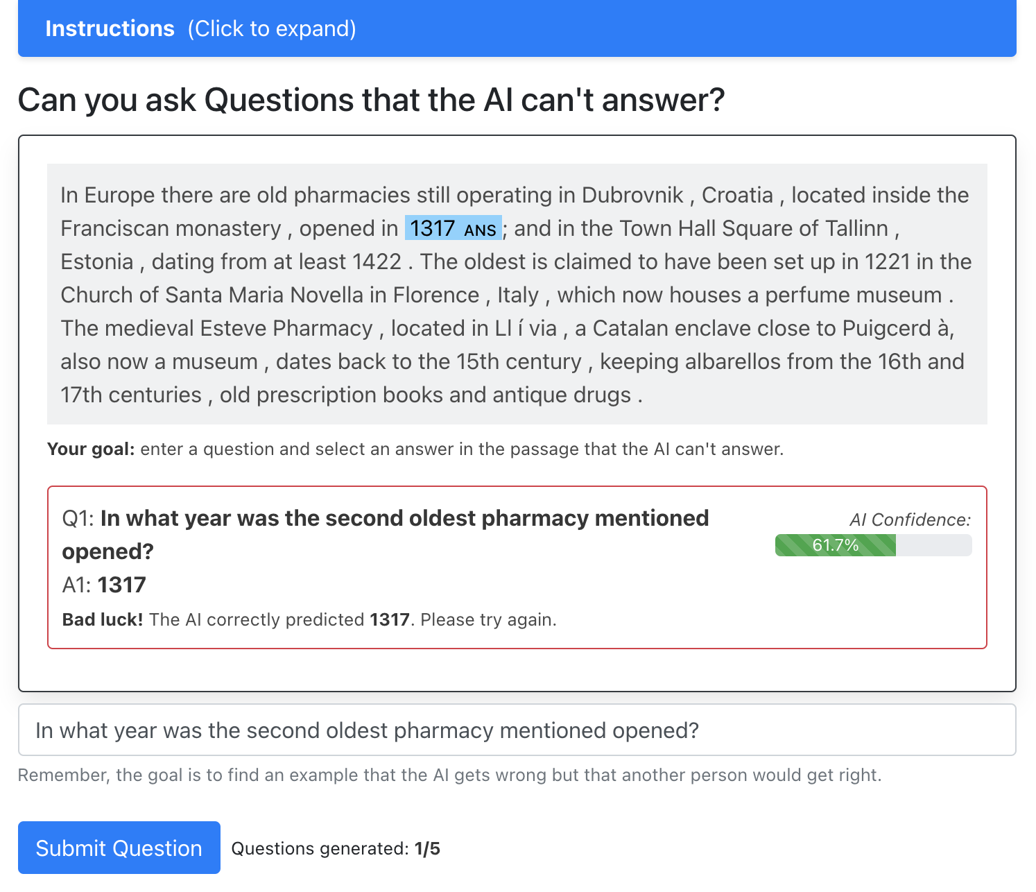
Figure 2: The Adversarial Human Evaluation Interface.

MRQA in-domain

Model

SQuAD

NewsQA

TriviaQA

SearchQA

HotpotQA

NQ

Avg

EM

F${}_{\text{1}}$

EM

F${}_{\text{1}}$

EM

F${}_{\text{1}}$

EM

F${}_{\text{1}}$

EM

F${}_{\text{1}}$

EM

F${}_{\text{1}}$

EM

F${}_{\text{1}}$

R${}_{\text{SQuAD}}$

84.1${}_{\text{\thinspace{1.3}}}$

90.4${}_{\text{\thinspace{1.3}}}$

41.0${}_{\text{\thinspace{1.2}}}$

57.5${}_{\text{\thinspace{1.6}}}$

60.2${}_{\text{\thinspace{0.7}}}$

69.0${}_{\text{\thinspace{0.8}}}$

16.0${}_{\text{\thinspace{1.8}}}$

20.8${}_{\text{\thinspace{2.7}}}$

53.6${}_{\text{\thinspace{0.8}}}$

68.9${}_{\text{\thinspace{0.8}}}$

40.5${}_{\text{\thinspace{2.7}}}$

58.5${}_{\text{\thinspace{2.0}}}$

49.2

60.9

R${}_{\text{SQuAD+AQA}}$

84.4${}_{\text{\thinspace{1.0}}}$

90.2${}_{\text{\thinspace{1.1}}}$

41.7${}_{\text{\thinspace{1.6}}}$

58.0${}_{\text{\thinspace{1.7}}}$

62.7${}_{\text{\thinspace{0.4}}}$

70.8${}_{\text{\thinspace{0.3}}}$

20.6${}_{\text{\thinspace{2.9}}}$

25.5${}_{\text{\thinspace{3.6}}}$

56.3${}_{\text{\thinspace{1.1}}}$

72.0${}_{\text{\thinspace{1.0}}}$

54.4${}_{\text{\thinspace{0.5}}}$

68.7${}_{\text{\thinspace{0.4}}}$

53.3

64.2

SynQA

88.8${}_{\text{\thinspace{0.3}}}$

94.3${}_{\text{\thinspace{0.2}}}$

42.9${}_{\text{\thinspace{1.6}}}$

60.0${}_{\text{\thinspace{1.4}}}$

62.3${}_{\text{\thinspace{1.1}}}$

70.2${}_{\text{\thinspace{1.1}}}$

23.7${}_{\text{\thinspace{3.7}}}$

29.5${}_{\text{\thinspace{4.4}}}$

59.8${}_{\text{\thinspace{1.1}}}$

75.3${}_{\text{\thinspace{1.0}}}$

55.1${}_{\text{\thinspace{1.0}}}$

68.7${}_{\text{\thinspace{0.8}}}$

55.4

66.3

SynQA${}_{\text{Ext}}$

89.0${}_{\text{\thinspace{0.3}}}$

94.3${}_{\text{\thinspace{0.2}}}$

46.2${}_{\text{\thinspace{0.9}}}$

63.1${}_{\text{\thinspace{0.8}}}$

58.1${}_{\text{\thinspace{1.8}}}$

65.5${}_{\text{\thinspace{1.9}}}$

28.7${}_{\text{\thinspace{3.2}}}$

34.3${}_{\text{\thinspace{4.1}}}$

59.6${}_{\text{\thinspace{0.6}}}$

75.5${}_{\text{\thinspace{0.4}}}$

55.3${}_{\text{\thinspace{1.1}}}$

68.8${}_{\text{\thinspace{0.9}}}$

56.2

66.9

MRQA out-of-domain

Model

BioASQ

DROP

DuoRC

RACE

RelationExt.

TextbookQA

Avg

EM

F${}_{\text{1}}$

EM

F${}_{\text{1}}$

EM

F${}_{\text{1}}$

EM

F${}_{\text{1}}$

EM

F${}_{\text{1}}$

EM

F${}_{\text{1}}$

EM

F${}_{\text{1}}$

R${}_{\text{SQuAD}}$

53.2${}_{\text{\thinspace{1.1}}}$

68.6${}_{\text{\thinspace{1.4}}}$

39.8${}_{\text{\thinspace{2.6}}}$

52.7${}_{\text{\thinspace{2.2}}}$

49.3${}_{\text{\thinspace{0.7}}}$

60.3${}_{\text{\thinspace{0.8}}}$

35.1${}_{\text{\thinspace{1.0}}}$

47.8${}_{\text{\thinspace{1.2}}}$

74.1${}_{\text{\thinspace{3.0}}}$

84.4${}_{\text{\thinspace{2.9}}}$

35.0${}_{\text{\thinspace{3.8}}}$

44.2${}_{\text{\thinspace{3.7}}}$

47.7

59.7

R${}_{\text{SQuAD+AQA}}$

54.6${}_{\text{\thinspace{1.2}}}$

69.4${}_{\text{\thinspace{0.8}}}$

59.8${}_{\text{\thinspace{1.3}}}$

68.4${}_{\text{\thinspace{1.5}}}$

51.8${}_{\text{\thinspace{1.1}}}$

62.2${}_{\text{\thinspace{1.0}}}$

38.4${}_{\text{\thinspace{0.9}}}$

51.6${}_{\text{\thinspace{0.9}}}$

75.4${}_{\text{\thinspace{2.3}}}$

85.8${}_{\text{\thinspace{2.4}}}$

40.1${}_{\text{\thinspace{3.1}}}$

48.2${}_{\text{\thinspace{3.6}}}$

53.3

64.3

SynQA

55.1${}_{\text{\thinspace{1.5}}}$

68.7${}_{\text{\thinspace{1.2}}}$

64.3${}_{\text{\thinspace{1.5}}}$

72.5${}_{\text{\thinspace{1.7}}}$

51.7${}_{\text{\thinspace{1.3}}}$

62.1${}_{\text{\thinspace{0.9}}}$

40.2${}_{\text{\thinspace{1.2}}}$

54.2${}_{\text{\thinspace{1.3}}}$

78.1${}_{\text{\thinspace{0.2}}}$

87.8${}_{\text{\thinspace{0.2}}}$

40.2${}_{\text{\thinspace{1.3}}}$

49.2${}_{\text{\thinspace{1.5}}}$

54.9

65.8

SynQA${}_{\text{Ext}}$

54.9${}_{\text{\thinspace{1.3}}}$

68.5${}_{\text{\thinspace{0.9}}}$

64.9${}_{\text{\thinspace{1.1}}}$

73.0${}_{\text{\thinspace{0.9}}}$

48.8${}_{\text{\thinspace{1.2}}}$

58.0${}_{\text{\thinspace{1.2}}}$

38.6${}_{\text{\thinspace{0.4}}}$

52.2${}_{\text{\thinspace{0.6}}}$

78.9${}_{\text{\thinspace{0.4}}}$

88.6${}_{\text{\thinspace{0.2}}}$

41.4${}_{\text{\thinspace{1.1}}}$

50.2${}_{\text{\thinspace{1.0}}}$

54.6

65.1

Table 8: Domain generalisation results on the in-domain (top) and out-of-domain (bottom) subsets of MRQA.

While existing robustness measures provide valuable insight into model behaviour, they fail to capture how robust a model might be in a production setting. We use Dynabench Kiela et al. (2021), a research platform for dynamic benchmarking and evaluation, to measure model robustness in an adversarial human evaluation setting. This allows for live interaction between the model and human annotator, and more closely simulates realistic and challenging scenarios a deployed system might encounter, compared to evaluation on static datasets.

We set up the experiment as a randomised controlled trial where annotators are randomly allocated to interact with each of our four final models based on a hash of their annotator identifier. We run the experiment through Amazon Mechanical Turk (AMT) using Mephisto. Workers (see Appendix I) are first required to complete an onboarding phase to ensure familiarity with the interface, and are then required to ask five questions of the model. We pay $0.20 per question and given a strong incentive to try to beat the model with a $0.50 bonus for each validated question that the model fails to answer correctly. The model identity is kept hidden and workers are awarded an equal base pay irrespective of the model-in-the-loop to avoid creating an incentive imbalance. Each annotator is allowed to write at most 50 questions, to avoid having a few productive annotators dominate our findings. All model-fooling examples are further validated by an expert annotator. We skip validation of questions the model answered correctly, as manual validation of a sample of 50 such examples found that all are valid, suggesting that the QA model’s ability to answer them is a good indicator of their validity.

We measure performance as the validated model error rate (vMER), that is, the percentage of validated examples that the model fails to answer correctly. Despite limiting the number of collected examples to 50 per annotator, there is still the potential of an imbalance in the number of QA pairs produced by each annotator. In order to eliminate annotator effect as a potential confounder, we propose using the macro-averaged validated model error rate (mvMER) over annotators, defined as:

$$\text{mvMER}=\frac{1}{n_{ann}}\sum^{n_{ann}}_{i=1}{\frac{\text{validated model errors}_{i}}{\text{number of examples}_{i}}}$$

We find that SynQA roughly halves the model error rate compared to R${}_{\text{SQuAD+AQA}}$ from 17.6% to 8.8% (see Table 7, further details in Appendix I), meaning that it is considerably harder for human adversaries to ask questions that the model cannot answer. While SynQA${}_{\text{Ext}}$ still considerably outperforms R${}_{\text{SQuAD+AQA}}$ at a 12.3% mvMER, we find that it is not as hard to beat as SynQA in this setting. A low model error rate also translates into increased challenges for the adversarial human annotation paradigm as the effort required for each model-fooling example increases, and provides motivation to expand the current extractive QA task beyond single answer spans on short passages.

These findings further suggest that while static adversarial benchmarks are a good evaluation proxy, performance gains on these may be underestimating the effect on model robustness in a setting involving direct interaction between the models-in-the-loop and human adversaries.

5 Discussion and Conclusion

In this work, we develop a synthetic adversarial data generation pipeline for QA, identify the best components, and evaluate on a variety of robustness measures. We propose novel approaches for answer candidate selection, adversarial question generation, and synthetic example filtering and re-labelling, demonstrating improvements over existing methods. Furthermore, we evaluate the final models on three existing robustness measures and achieve state-of-the-art results on AdversarialQA, improved learnability of various comprehension skills for CheckList, and improved domain generalisation for the suite of MRQA tasks.

We then put the synthetically-augmented models back in-the-loop in an adversarial human evaluation setting to assess whether these models are actually harder for a human adversary to beat.

We find that our best synthetically-augmented model is roughly twice as hard to beat. Our findings suggest that synthetic adversarial data generation can be used to improve QA model robustness, both when measured using standard methods and when evaluated directly against human adversaries.

Looking forward, the methods explored in this work could also be used to scale the dynamic adversarial annotation process in multiple ways. Synthetic adversarial data generation could facilitate faster iteration over rounds of adversarial human annotation as it reduces the amount of human data required to effectively train an improved QA model. Generative models could also help guide or inspire human annotators as they try to come up with more challenging examples. Furthermore, while our work focuses on improving adversarial robustness, this approach is not limited to the adversarial setting. We believe that our findings can motivate similar investigations for tasks where data acquisition can be challenging due to limited resources, or for improving different aspects of robustness, for example for model bias mitigation.

6 Ethical Considerations

We collect an evaluation dataset as a part of the adversarial human evaluation process. The passages are sourced from the SQuAD1.1 dataset distributed under the CC BY-SA 4.0 license. As described in the main text, we designed our incentive structure to ensure that crowdworkers were fairly compensated. Full details are provided in the main text and Appendix I. Our datasets focus on the English language. As this data is not collected for the purpose of designing NLP applications, we do not foresee any risks associated with the use of this data.

Appendix A Further Details on Passage Selection

Passages are sourced from SQuAD1.1, and are therefore from Wikipedia. For training answer candidate selection models and question generation models, we use a subset of 10,000 examples from the SQuAD1.1 training set asked on 2,596 of the 18,891 available training passages. This ensures that both the answer candidate selection and question generation models do not simply reproduce their respective training sets. Bartolo et al. (2020) split the SQuAD1.1 dev set into a dev and test set, with passages allocated between the two. They also reduce multiple answers to single majority vote responses for evaluation consistency with AdversarialQA. These two splits are referred to as $\mathcal{D_{\mathrm{SQuAD}}}$^dev and $\mathcal{D_{\mathrm{SQuAD}}}$^test. We use $\mathcal{D_{\mathrm{SQuAD}}}$^dev and the AdversarialQA dev sets for validation, and report results on $\mathcal{D_{\mathrm{SQuAD}}}$^test and the AdversarialQA test sets. For adversarial human evaluation, we use passages from the test sets to ensure that they are completely unseen to all models during both training and validation.

Appendix B Manual Answerability Analysis

For the manual answerability analysis, we define answerability by the following criteria: (i) The question must be answerable from a single continuous span in the passage; (ii) There must be only one valid (or clearly one most valid) answer (e.g. in the case of a co-reference the canonical entity name should be the answer); (iii) A human should be able to answer the question correctly given sufficient time; and (iv) The correct answer is the one on which the model was conditioned during question generation.

Appendix C Further Details on Answer Candidate Selection

Dataset statistics for the passage-aligned splits are shown in Table 9.

Split	#Passages	#Ans per passage	% Overlapping answers	% Passages w/ overlaps
Train	2596	13.0	29.2%	90.4%
Dev	416	13.6	35.3%	97.4%
Test	409	13.5	33.3%	94.1%

Table 9: Dataset statistics for answer candidate selection showing high answer overlap.

Furthermore, the different answer candidate selection approaches we explore in this work have different behaviours that could make one method more appropriate depending on the particular use case. To facilitate this process, we provide some example answer candidates of each of the methods in Table 11.

Appendix D Further Details on Question Diversity

In order to provide training signal diversity to the downstream QA model, we experiment with a range of diversity decoding techniques and hyper-parameters. Specifically, we explore standard beam search with $beam\_size\in\{1,3,5,10\}$, number of questions to generate per example with $nbest\in\{1,3,5,10\}$, diverse beam search with $beam\_strength\in\{0.1,0.3,0.5,0.7,0.9,1.0\}$, and nucleus sampling with $top_{p}\in\{0.1,0.5,0.75\}$.

We observe minimal variation in downstream performance (see Table 13) as a result of question decoding strategy, with the best downstream results obtained using nucleus sampling ($top_{p}=0.75$). However, we also obtain similar downstream results with standard beam search using a beam size of 5. We find that, given the same computational resources, standard beam search is roughly twice as efficient, with minimal performance drop when compared to nucleus sampling, and therefore opt for this approach for our following experiments.

Appendix E Controlling for Data Size

Since the synthetic data generation process allows for scale to a large number of unseen passages, at the limit the bottleneck becomes the quality of generating data rather than quantity. Due to this, we provide results for experiments controlling for dataset size for both answer candidate selection (see Table 12) and filtering method (see Table 14). Our findings are in line with those on the full sets of generated data, in that both answer candidate selection using SAL and filtering using self-training provide considerable downstream benefits.

Appendix F A Note on Data Efficiency

It is challenging to compare the efficiency of the synthetic generation process to manually collecting additional data. Figure 3 shows that, for RoBERTa${}_{\text{Large}}$, performance starts to converge when trained on around 5-6k manually-collected adversarial examples. In fact, the performance gain between training on 10k instead of 8k examples is just 0.5F${}_{\text{1}}$ on the overall AdversarialQA test set. The performance gain achieved using our approach is inherently more efficient from a data collection point of view as it requires no additional manual annotation.

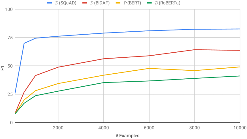
Figure 3: F1-scores on the respective test datasets for RoBERTa${}_{\text{Large}}$ trained on varying amounts of human-annotated adversarial training data.

Appendix G AdversarialQA Dev Set Results

Results for the final models on the AdversarialQA validations sets are shown in Table 15.

Appendix H Results on CheckList

We provide a breakdown of results by comprehension skill and example model failure cases on CheckList in Table J.

Appendix I Adversarial Human Evaluation

For adversarial human evaluation, crowdworkers are required to be based in Canada, the UK, or the US, have a Human Intelligence Task (HIT) Approval Rate greater than $98\%$, and have previously completed at least 1,000 HITs.

We provide a breakdown of results from the Adversarial Human Evaluation experiments in Table 10, showing the number of annotators (#Ann.), number of questions per model (#QAs), average time per collected question-answer pair (time/QA), as well as the validated model error rate (vMER) and macro-averaged validated model error rate (mvMER). We also show some examples of questions that fool each model in Table 18.

Model	#Ann.	#QAs	time/QA	vMER	mvMER
R${}_{\text{SQuAD}}$	33	705	97.4s	21.4%	20.7%
R${}_{\text{SQuAD+AQA}}$	40	798	95.9s	15.5%	17.6%
SynQA	32	820	112.6s	6.7%	8.8%
SynQA${}_{\text{Ext}}$	30	769	85.2s	9.2%	12.3%

Table 10: Adversarial Human Evaluation results for the four final models.

Appendix J Results for ELECTRA_Large

In Table 16 we show results for ELECTRA_Large demonstrating similar performance gains as those seen for RoBERTa${}_{\text{Large}}$ when using the additional synthetic data. We show results for a single initialisation due to computational cost. We also note that we use the same synthetic training data (i.e. using six RoBERTa${}_{\text{Large}}$ RC models for self-training relabelling) and two-stage fine-tuning setup.

The synthetically-augmented ELECTRA_Large model also shows considerable domain generalisation improvements on MRQA achieving 94.5F${}_{\text{1}}$ on SQuAD; 66.6F${}_{\text{1}}$ on NewsQA; 72.7F${}_{\text{1}}$ on TriviaQA; 53.8F${}_{\text{1}}$ on SearchQA; 73.3F${}_{\text{1}}$ on HotpotQA; 72.3F${}_{\text{1}}$ on NQ; 71.4F${}_{\text{1}}$ on BioASQ; 72.6F${}_{\text{1}}$ on DROP; 65.2F${}_{\text{1}}$ on DuoRC; 56.2F${}_{\text{1}}$ on RACE; 89.3F${}_{\text{1}}$ on RelationExtraction; and 59.8F${}_{\text{1}}$ on TextbookQA. Further model details can be found at https://dynabench.org/models/109.

Context:	Super Bowl 50 was an American football game to determine the champion of the National Football League (NFL) for the 2015 season. The American Football Conference (AFC) champion Denver Broncos defeated the National Football Conference (NFC) champion Carolina Panthers 24–10 to earn their third Super Bowl title. The game was played on February 7, 2016, at Levi’s Stadium in the San Francisco Bay Area at Santa Clara, California. As this was the 50th Super Bowl, the league emphasized the "golden anniversary" with various gold-themed initiatives, as well as temporarily suspending the tradition of naming each Super Bowl game with Roman numerals (under which the game would have been known as "Super Bowl L"), so that the logo could prominently feature the Arabic numerals 50.
Ground Truth	’Super Bowl’, ’the 2015 season’, ’2015’, ’American Football Conference’, ’Denver Broncos’, ’Denver Broncos defeated the National Football Conference (NFC) champion Carolina Panthers 24–10’, ’Carolina Panthers’, ’24–10’, ’February 7’, ’February 7, 2016’, ’2016’, "Levi’s Stadium", "Levi’s Stadium in the San Francisco Bay Area at Santa Clara", "Levi’s Stadium in the San Francisco Bay Area at Santa Clara, California", ’Santa Clara’, ’Santa Clara, California’, ’the league emphasized the "golden anniversary" with various gold-themed initiatives, as well as temporarily suspending the tradition of naming each Super Bowl game with Roman numerals (under which the game would have been known as "Super Bowl L"), so that the logo could prominently feature the Arabic numerals 50’, ’gold’, ’golden anniversary’, ’gold-themed’, ’Super Bowl L’, ’L’
POS Extended	’Super’, ’50’, ’Super Bowl’, ’Bowl’, ’American’, ’an American football game’, ’the National Football League’, ’the champion’, ’NFL’, ’the 2015 season’, ’(NFL’, ’The American Football Conference’, ’football’, ’AFC’, ’The American Football Conference (AFC) champion Denver Broncos’, ’game’, ’Denver Broncos’, ’the National Football Conference (NFC) champion’, ’the National Football Conference’, ’their third Super Bowl title’, ’Carolina Panthers’, ’The game’, ’third’, ’February’, ’champion’, "Levi’s Stadium", ’February 7, 2016’, ’the San Francisco Bay Area’, ’Santa Clara’, ’the National Football League (NFL)’, ’National’, ’California’, ’Football’, ’the 50th Super Bowl’, ’League’, ’the league’, ’50th’, ’the "golden anniversary’, ’various gold-themed initiatives’, ’the tradition’, ’Roman’, ’each Super Bowl game’, ’Arabic’, ’Roman numerals’, ’2015’, ’the game’, ’season’, ’Super Bowl L’, ’the logo’, ’the Arabic numerals’, ’Conference’, ’Denver’, ’Broncos’, ’NFC’, ’Carolina’, ’Panthers’, ’24–10’, ’title’, ’February 7, 2016,’, ’7’, ’2016’, ’Levi’, "Levi’s Stadium in the San Francisco Bay Area at Santa Clara, California", ’Stadium’, ’the San Francisco Bay Area at Santa Clara, California’, ’San’, ’Francisco’, ’Bay’, ’Area’, ’Santa’, ’Santa Clara, California’, ’Clara’, ’league’, ’golden’, ’anniversary’, ’various’, ’gold’, ’themed’, ’initiatives’, ’tradition’, ’Roman numerals (under which the game would have been known as "Super Bowl L"’, ’numerals’, ’L’, ’logo’
Noun Chunks	’Super Bowl’, ’an American football game’, ’the champion’, ’the National Football League’, ’(NFL’, ’the 2015 season’, ’The American Football Conference (AFC) champion Denver Broncos’, ’the National Football Conference (NFC) champion’, ’their third Super Bowl title’, ’The game’, ’February’, "Levi’s Stadium", ’the San Francisco Bay Area’, ’Santa Clara’, ’California’, ’the 50th Super Bowl’, ’the league’, ’the "golden anniversary’, ’various gold-themed initiatives’, ’the tradition’, ’each Super Bowl game’, ’Roman numerals’, ’the game’, ’Super Bowl L’, ’the logo’, ’the Arabic numerals’
Named Entities	[’50’, ’American’, ’the National Football League’, ’NFL’, ’the 2015 season’, ’The American Football Conference’, ’AFC’, ’Denver Broncos’, ’the National Football Conference’, ’Carolina Panthers’, ’third’, ’Super Bowl’, ’February 7, 2016’, "Levi’s Stadium", ’the San Francisco Bay Area’, ’Santa Clara’, ’California’, ’50th’, ’Roman’, ’Arabic’]
Span Extraction, k=15	’Denver Broncos’, ’Denver Broncos defeated the National Football Conference (NFC) champion Carolina Panthers’, "Levi’s Stadium", "February 7, 2016, at Levi’s Stadium", ’February 7, 2016,’, ’Carolina Panthers’, ’Carolina Panthers 24–10 to earn their third Super Bowl title. The game was played on February 7, 2016,’, "Levi’s Stadium in the San Francisco Bay Area at Santa Clara, California.", ’Denver Broncos defeated the National Football Conference (NFC) champion Carolina Panthers 24–10’, "February 7, 2016, at Levi’s Stadium in the San Francisco Bay Area at Santa Clara, California.", "24–10 to earn their third Super Bowl title. The game was played on February 7, 2016, at Levi’s Stadium", ’24–10 to earn their third Super Bowl title. The game was played on February 7, 2016,’, ’Carolina Panthers 24–10’, ’Santa Clara, California.’, ’American Football Conference (AFC) champion Denver Broncos’
BART${}_{\text{ans}}$, k=15	’NFL’, ’the "golden anniversary"’, ’American Football Conference’, ’Super Bowl 50’, ’San Francisco Bay Area’, ’National Football League’, ’Super Bowl L’, ’Super Bowl’, "Levi’s Stadium", ’National Football Conference’, ’Roman numerals’, ’Denver Broncos’, ’Gold’, ’2016’, ’The game was played’
SAL (ours)	’Super Bowl 50’, ’American’, ’American football’, ’National Football League’, ’Football’, ’Football League’, ’American Football Conference’, ’American Football Conference (AFC)’, ’American Football Conference (AFC) champion Denver Broncos’, ’Denver Broncos’, ’National Football Conference’, ’National Football Conference (NFC)’, ’National Football Conference (NFC) champion Carolina Panthers’, ’Carolina Panthers’, ’24’, ’10’, ’third’, ’February 7, 2016’, "Levi’s Stadium", ’San Francisco Bay Area’, ’Santa Clara’, ’gold’, ’naming each Super Bowl game with Roman numerals’, ’Roman numerals’, ’Super Bowl L’, ’so that the logo could prominently feature the Arabic numerals 50’

Table 11: Examples of answer candidates selected by different answer selection approaches.

Method	#QA pairs	$\mathcal{D_{\mathrm{SQuAD}}}$		$\mathcal{D_{\mathrm{BiDAF}}}$		$\mathcal{D_{\mathrm{BERT}}}$		$\mathcal{D_{\mathrm{RoBERTa}}}$
		EM	F${}_{\text{1}}$	EM	F${}_{\text{1}}$	EM	F${}_{\text{1}}$	EM	F${}_{\text{1}}$
POS Extended	87000	54.0	72.7	32.0	45.9	27.9	38.3	19.4	27.0
Noun Chunks	87000	42.1	62.7	25.8	40.0	21.2	30.0	17.0	25.1
Named Entities	87000	55.0	69.9	29.1	40.4	26.7	36.0	17.9	24.1
Span Extraction	87000	64.2	79.7	34.1	50.8	25.9	38.0	16.4	27.1
SAL (ours)	87000	67.1	82.0	40.5	55.2	36.0	45.6	23.5	33.5
SAL threshold (ours)	87000	68.4	82.0	43.9	58.6	33.2	43.5	25.2	33.9

Table 12: Downstream QA test results for different answer candidate selection methods combined with a question generator, controlling for dataset size.

Decoding Method	#QA pairs	$\mathcal{D_{\mathrm{SQuAD}}}$		$\mathcal{D_{\mathrm{BiDAF}}}$		$\mathcal{D_{\mathrm{BERT}}}$		$\mathcal{D_{\mathrm{RoBERTa}}}$
		EM	F${}_{\text{1}}$	EM	F${}_{\text{1}}$	EM	F${}_{\text{1}}$	EM	F${}_{\text{1}}$
Beam Search ($beam\_size=1$)	87,598	67.8	80.7	40.0	55.2	30.4	41.4	17.6	26.8
Beam Search ($beam\_size=3$)	87,598	69.0	82.3	40.4	55.8	30.0	40.1	20.8	30.8
Beam Search ($beam\_size=5$)	87,598	69.3	83.0	39.8	54.0	31.4	42.4	19.4	30.1
Beam Search ($beam\_size=10$)	87,598	69.6	82.7	40.5	54.1	30.4	41.0	18.8	29.0
Diverse Beam Search ($beam\_strength=0.1$)	87,598	68.8	81.8	41.3	56.2	31.1	40.9	19.2	29.7
Diverse Beam Search ($beam\_strength=0.3$)	87,598	67.7	80.8	40.1	53.4	31.6	41.3	18.8	28.0
Diverse Beam Search ($beam\_strength=0.5$)	87,598	68.5	81.7	40.6	55.2	31.0	41.1	20.3	28.8
Diverse Beam Search ($beam\_strength=0.7$)	87,598	69.0	82.5	40.1	55.1	31.1	41.9	18.4	27.6
Diverse Beam Search ($beam\_strength=0.9$)	87,598	68.4	81.5	41.2	55.8	32.6	42.2	19.0	29.1
Diverse Beam Search ($beam\_strength=1.0$)	87,598	68.1	81.4	39.4	53.8	30.9	41.8	17.3	27.2
Nucleus Sampling ($top_{p}=0.1$)	87,598	68.4	81.6	42.0	56.7	31.9	42.1	18.7	28.1
Nucleus Sampling ($top_{p}=0.5$)	87,598	68.1	81.4	40.8	55.1	31.6	41.4	19.2	28.5
Nucleus Sampling ($top_{p}=0.75$)	87,598	69.8	83.2	41.1	56.3	31.1	42.2	21.4	31.9

Table 13: Downstream QA test results for different question diversity decoding strategies and hyper-parameter settings. Synthetic data for these experiments was generated on the human-annotated answers and using the generator trained on SQuAD_10k + $\mathcal{D_{\mathrm{AQA}}}$.

Filtering Method	#QA pairs	$\mathcal{D_{\mathrm{SQuAD}}}$		$\mathcal{D_{\mathrm{BiDAF}}}$		$\mathcal{D_{\mathrm{BERT}}}$		$\mathcal{D_{\mathrm{RoBERTa}}}$
		EM	F${}_{\text{1}}$	EM	F${}_{\text{1}}$	EM	F${}_{\text{1}}$	EM	F${}_{\text{1}}$
Answer Candidate Conf. ($thresh=0.6$)	15,000	65.3	79.9	39.7	53.3	30.9	41.2	20.1	30.6
Question Generator Conf. ($thresh=0.5$)	15,000	65.0	80.0	38.7	53.8	29.4	40.8	20.6	31.8
Influence Functions	15,000	63.8	79.3	37.2	53.1	28.4	39.0	19.1	29.7
Ensemble Roundtrip Consistency ($6/6$ correct)	15,000	70.4	83.5	44.0	57.4	32.5	44.1	22.3	31.0
Self-training (ST)	15,000	71.5	84.3	42.4	56.2	35.4	45.5	23.6	33.0
Answer Candidate Conf. ($thresh=0.5$) & ST	15,000	71.0	84.0	47.1	60.6	32.3	43.4	24.9	34.9

Table 14: Downstream QA test results for different question-answer pair filtering strategies, showing the best hyper-parameter setting for each method, controlling for dataset size.

Model	Training Data	$\mathcal{D_{\mathrm{BiDAF}}}$		$\mathcal{D_{\mathrm{BERT}}}$		$\mathcal{D_{\mathrm{RoBERTa}}}$
		EM	F${}_{\text{1}}$	EM	F${}_{\text{1}}$	EM	F${}_{\text{1}}$
R${}_{\text{SQuAD}}$	SQuAD	51.8${}_{\text{\thinspace{1.4}}}$	65.5${}_{\text{\thinspace{0.8}}}$	30.2${}_{\text{\thinspace{1.8}}}$	42.2${}_{\text{\thinspace{1.6}}}$	15.1${}_{\text{\thinspace{2.4}}}$	24.8${}_{\text{\thinspace{2.8}}}$
R${}_{\text{SQuAD+AQA}}$	$\uparrow$ + AQA	59.5${}_{\text{\thinspace{1.1}}}$	72.7${}_{\text{\thinspace{0.9}}}$	49.4${}_{\text{\thinspace{1.0}}}$	60.4${}_{\text{\thinspace{0.9}}}$	36.4${}_{\text{\thinspace{1.6}}}$	46.6${}_{\text{\thinspace{1.9}}}$
SynQA	$\uparrow$ + SynQA${}_{\text{SQuAD}}$	63.9${}_{\text{\thinspace{1.0}}}$	76.6${}_{\text{\thinspace{0.9}}}$	54.5${}_{\text{\thinspace{1.8}}}$	65.8${}_{\text{\thinspace{2.0}}}$	42.7${}_{\text{\thinspace{1.5}}}$	52.6${}_{\text{\thinspace{1.5}}}$
SynQA${}_{\text{Ext}}$	$\uparrow$ + SynQA${}_{\text{Ext}}$	63.5${}_{\text{\thinspace{0.2}}}$	75.7${}_{\text{\thinspace{0.4}}}$	54.2${}_{\text{\thinspace{0.9}}}$	65.5${}_{\text{\thinspace{0.6}}}$	41.2${}_{\text{\thinspace{0.4}}}$	51.9${}_{\text{\thinspace{0.4}}}$

Table 15: Validation set results for RoBERTa${}_{\text{Large}}$ trained on different datasets, and augmented with synthetic data. AQA is the AdversarialQA data consisting of the combined $\mathcal{D_{\mathrm{BiDAF}}}$, $\mathcal{D_{\mathrm{BERT}}}$, and $\mathcal{D_{\mathrm{RoBERTa}}}$ from Bartolo et al. (2020). We report the mean and standard deviation (subscript) over 6 runs with different random seeds.

Training Data	$\mathcal{D_{\mathrm{SQuAD}}}$		$\mathcal{D_{\mathrm{BiDAF}}}$		$\mathcal{D_{\mathrm{BERT}}}$		$\mathcal{D_{\mathrm{RoBERTa}}}$
	EM	F${}_{\text{1}}$	EM	F${}_{\text{1}}$	EM	F${}_{\text{1}}$	EM	F${}_{\text{1}}$
SQuAD + AQA	77.1	88.5	62.2	76.5	58.2	68.1	46.9	58.0
SQuAD + AQA + SynQA${}_{\text{SQuAD}}$	77.0	88.6	63.5	76.9	60.0	70.3	50.1	61.0

Table 16: Test set results for ELECTRA_Large trained on the SQuAD and AdversarialQA datasets, and then augmented with synthetic data. It is worth noting that ELECTRA_Large without augmentation performs similarly to RoBERTa${}_{\text{Large}}$ with synthetic augmentation, and synthetically augmenting ELECTRA_Large further provides performance gains of up to 3F${}_{\text{1}}$ on the most challenging questions.

	Test Description	R${}_{\text{SQuAD}}$	R${}_{\text{SQuAD+AQA}}$	SynQA	SynQA${}_{\text{Ext}}$	Example Failure cases (with expected behaviour and model prediction)
Vocab	A is COMP than B. Who is more / less COMP?	19.1${}_{\text{\thinspace{8.2}}}$	4.6${}_{\text{\thinspace{4.6}}}$	6.7${}_{\text{\thinspace{5.3}}}$	2.5${}_{\text{\thinspace{1.7}}}$	$\begin{array}[]{l}\parbox{344.27852pt}{{C:} Christina is younger than Joshua.}\\[2.0pt] \parbox{344.27852pt}{ {Q:} Who is less young? {A:} \hbox{\pagecolor{lightgrey}\vrule width=0.0pt,height=0.0pt,depth=0.0pt{\color[rgb]{0,0,0}Joshua}\/} ~{}~{}{M:} Christina }\end{array}$
	Intensifiers (very, super, extremely) and reducers (somewhat, kinda, etc)?	70.8${}_{\text{\thinspace{13.2}}}$	72.6${}_{\text{\thinspace{16.0}}}$	78.4${}_{\text{\thinspace{15.3}}}$	79.8${}_{\text{\thinspace{14.3}}}$	$\begin{array}[]{l}\parbox{344.27852pt}{{C:} Timothy is a little ambitious about the project. Melissa is ambitious about the project.}\\[2.0pt] \parbox{344.27852pt}{ {Q:} Who is least ambitious about the project? {A:} \hbox{\pagecolor{lightgrey}\vrule width=0.0pt,height=0.0pt,depth=0.0pt{\color[rgb]{0,0,0}Timothy}\/} ~{}~{}{M:} Melissa }\end{array}$
Taxonomy	Size, shape, age, color	39.5${}_{\text{\thinspace{3.0}}}$	16.2${}_{\text{\thinspace{4.8}}}$	9.0${}_{\text{\thinspace{2.9}}}$	8.2${}_{\text{\thinspace{1.7}}}$	$\begin{array}[]{l}\parbox{344.27852pt}{{C:} There is a tiny oval thing in the room.}\\[2.0pt] \parbox{344.27852pt}{ {Q:} What size is the thing? {A:} \hbox{\pagecolor{lightgrey}\vrule width=0.0pt,height=0.0pt,depth=0.0pt{\color[rgb]{0,0,0}tiny}\/} ~{}~{}{M:} oval }\end{array}$
	Profession vs nationality	68.8${}_{\text{\thinspace{8.7}}}$	37.5${}_{\text{\thinspace{9.9}}}$	23.7${}_{\text{\thinspace{11.7}}}$	5.9${}_{\text{\thinspace{1.6}}}$	$\begin{array}[]{l}\parbox{344.27852pt}{{C:} Lauren is a Japanese adviser.}\\[2.0pt] \parbox{344.27852pt}{ {Q:} What is Lauren's job? {A:} \hbox{\pagecolor{lightgrey}\vrule width=0.0pt,height=0.0pt,depth=0.0pt{\color[rgb]{0,0,0}adviser}\/} ~{}~{}{M:} a Japanese adviser }\end{array}$
	Animal vs Vehicle	9.6${}_{\text{\thinspace{0.0}}}$	2.1${}_{\text{\thinspace{0.0}}}$	2.6${}_{\text{\thinspace{0.0}}}$	0.0${}_{\text{\thinspace{0.0}}}$	$\begin{array}[]{l}\parbox{344.27852pt}{{C:} Emily has a SUV and an iguana.}\\[2.0pt] \parbox{344.27852pt}{ {Q:} What animal does Emily have? {A:} \hbox{\pagecolor{lightgrey}\vrule width=0.0pt,height=0.0pt,depth=0.0pt{\color[rgb]{0,0,0}iguana}\/} ~{}~{}{M:} SUV }\end{array}$
	Animal vs Vehicle (Advanced)	3.3${}_{\text{\thinspace{2.4}}}$	1.0${}_{\text{\thinspace{1.0}}}$	2.9${}_{\text{\thinspace{1.7}}}$	2.7${}_{\text{\thinspace{2.5}}}$	$\begin{array}[]{l}\parbox{344.27852pt}{{C:} Rebecca bought a train. Christian bought a bull.}\\[2.0pt] \parbox{344.27852pt}{ {Q:} Who bought a vehicle? {A:} \hbox{\pagecolor{lightgrey}\vrule width=0.0pt,height=0.0pt,depth=0.0pt{\color[rgb]{0,0,0}Rebecca}\/} ~{}~{}{M:} Christian }\end{array}$
Synonyms	Basic synonyms	0.3${}_{\text{\thinspace{0.1}}}$	0.2${}_{\text{\thinspace{0.1}}}$	0.0${}_{\text{\thinspace{0.1}}}$	2.1${}_{\text{\thinspace{2.1}}}$	$\begin{array}[]{l}\parbox{344.27852pt}{{C:} Samuel is very intelligent. Samantha is very happy.}\\[2.0pt] \parbox{344.27852pt}{ {Q:} Who is joyful? {A:} \hbox{\pagecolor{lightgrey}\vrule width=0.0pt,height=0.0pt,depth=0.0pt{\color[rgb]{0,0,0}Samantha}\/} ~{}~{}{M:} Samuel }\end{array}$
	A is COMP than B. Who is antonym(COMP)? B	17.0${}_{\text{\thinspace{10.6}}}$	3.4${}_{\text{\thinspace{3.6}}}$	0.7${}_{\text{\thinspace{0.9}}}$	2.2${}_{\text{\thinspace{1.8}}}$	$\begin{array}[]{l}\parbox{344.27852pt}{{C:} Taylor is darker than Mary.}\\[2.0pt] \parbox{344.27852pt}{ {Q:} Who is lighter? {A:} \hbox{\pagecolor{lightgrey}\vrule width=0.0pt,height=0.0pt,depth=0.0pt{\color[rgb]{0,0,0}Mary}\/} ~{}~{}{M:} Taylor }\end{array}$
	A is more X than B. Who is more antonym(X)? B. Who is less X? B. Who is more X? A. Who is less antonym(X)? A.	99.7${}_{\text{\thinspace{0.6}}}$	72.8${}_{\text{\thinspace{8.4}}}$	81.6${}_{\text{\thinspace{6.6}}}$	93.4${}_{\text{\thinspace{5.4}}}$	$\begin{array}[]{l}\parbox{344.27852pt}{{C:} Emma is more cautious than Ethan.}\\[2.0pt] \parbox{344.27852pt}{ {Q:} Who is more brave? {A:} \hbox{\pagecolor{lightgrey}\vrule width=0.0pt,height=0.0pt,depth=0.0pt{\color[rgb]{0,0,0}Ethan}\/} ~{}~{}{M:} Emma }\end{array}$
Robustness	Swap adjacent characters in Q (typo)	12.5${}_{\text{\thinspace{1.5}}}$	12.8${}_{\text{\thinspace{0.9}}}$	7.0${}_{\text{\thinspace{1.0}}}$	8.1${}_{\text{\thinspace{0.5}}}$	$\begin{array}[]{l}\parbox{344.27852pt}{{C:} \ldots to trigger combustion. Oxygen is the oxidant, not the fuel, but nevertheless the source \ldots}\\[2.0pt] \parbox{344.27852pt}{ {Q:} Combustion is \hbox{\pagecolor{cdelback}\vrule width=0.0pt,height=0.0pt,depth=0.0pt{\color[rgb]{0.83,0.32,0.16}caused}\/} $\mathrel{\hbox{\rule[-0.2pt]{3.0pt}{0.4pt}}\mkern-4.0mu\hbox{\char 41\relax}}$ \hbox{\pagecolor{caddback}\vrule width=0.0pt,height=0.0pt,depth=0.0pt{\color[rgb]{0,0.47,0.34}causde}\/} by an oxidant and a fuel. What role does oxygen play in combustion? {A:} \hbox{\pagecolor{lightgrey}\vrule width=0.0pt,height=0.0pt,depth=0.0pt{\color[rgb]{0,0,0} \hbox{\pagecolor{lightgrey}\vrule width=0.0pt,height=0.0pt,depth=0.0pt{\color[rgb]{0,0,0}INV}\/}}\/} ~{}~{}{M:} \hbox{\pagecolor{cdelback}\vrule width=0.0pt,height=0.0pt,depth=0.0pt{\color[rgb]{0.83,0.32,0.16}oxidant, not the fuel}\/} $\mathrel{\hbox{\rule[-0.2pt]{3.0pt}{0.4pt}}\mkern-4.0mu\hbox{\char 41\relax}}$ \hbox{\pagecolor{caddback}\vrule width=0.0pt,height=0.0pt,depth=0.0pt{\color[rgb]{0,0.47,0.34}oxidant}\/} }\end{array}$
	Question contractions	3.6${}_{\text{\thinspace{1.4}}}$	5.0${}_{\text{\thinspace{1.3}}}$	1.6${}_{\text{\thinspace{0.6}}}$	1.8${}_{\text{\thinspace{0.5}}}$	$\begin{array}[]{l}\parbox{344.27852pt}{{C:} \ldots foliated, and folded. Even older rocks, such as the Acasta gneiss of the Slave craton in northwestern Canada, the oldest known rock in the world have been metamorphosed to \ldots}\\[2.0pt] \parbox{344.27852pt}{ {Q:} \hbox{\pagecolor{cdelback}\vrule width=0.0pt,height=0.0pt,depth=0.0pt{\color[rgb]{0.83,0.32,0.16}What is}\/} $\mathrel{\hbox{\rule[-0.2pt]{3.0pt}{0.4pt}}\mkern-4.0mu\hbox{\char 41\relax}}$ \hbox{\pagecolor{caddback}\vrule width=0.0pt,height=0.0pt,depth=0.0pt{\color[rgb]{0,0.47,0.34}What's}\/} the oldest known rock in the world? {A:} \hbox{\pagecolor{lightgrey}\vrule width=0.0pt,height=0.0pt,depth=0.0pt{\color[rgb]{0,0,0} \hbox{\pagecolor{lightgrey}\vrule width=0.0pt,height=0.0pt,depth=0.0pt{\color[rgb]{0,0,0}INV}\/}}\/} ~{}~{}{M:} \hbox{\pagecolor{cdelback}\vrule width=0.0pt,height=0.0pt,depth=0.0pt{\color[rgb]{0.83,0.32,0.16}the Acasta gneiss of the Slave craton}\/} $\mathrel{\hbox{\rule[-0.2pt]{3.0pt}{0.4pt}}\mkern-4.0mu\hbox{\char 41\relax}}$ \hbox{\pagecolor{caddback}\vrule width=0.0pt,height=0.0pt,depth=0.0pt{\color[rgb]{0,0.47,0.34}Slave craton}\/} }\end{array}$
	Add random sentence to context	14.9${}_{\text{\thinspace{3.3}}}$	14.5${}_{\text{\thinspace{1.8}}}$	6.3${}_{\text{\thinspace{1.0}}}$	8.4${}_{\text{\thinspace{0.8}}}$	$\begin{array}[]{l}\parbox{344.27852pt}{{C:} \hbox{\pagecolor{lightgrey}\vrule width=0.0pt,height=0.0pt,depth=0.0pt{\color[rgb]{0,0,0}Each digit will weigh 33 lb (15 kg) for a total of 66 lb (30 kg).}\/} The shape of the Rhine delta is \ldots The largest and southern main branch begins as Waal and continues as Boven Merwede ("Upper Merwede"), Beneden Merwede ("Lower Merwede"), Noord River ("North \ldots}\\[2.0pt] \parbox{344.27852pt}{ {Q:} What is the largest main branch of the Rhine? {A:} \hbox{\pagecolor{lightgrey}\vrule width=0.0pt,height=0.0pt,depth=0.0pt{\color[rgb]{0,0,0} \hbox{\pagecolor{lightgrey}\vrule width=0.0pt,height=0.0pt,depth=0.0pt{\color[rgb]{0,0,0}INV}\/}}\/} ~{}~{}{M:} \hbox{\pagecolor{cdelback}\vrule width=0.0pt,height=0.0pt,depth=0.0pt{\color[rgb]{0.83,0.32,0.16}Waal}\/} $\mathrel{\hbox{\rule[-0.2pt]{3.0pt}{0.4pt}}\mkern-4.0mu\hbox{\char 41\relax}}$ \hbox{\pagecolor{caddback}\vrule width=0.0pt,height=0.0pt,depth=0.0pt{\color[rgb]{0,0.47,0.34}Boven Merwede}\/} }\end{array}$
NER	Change name everywhere	9.1${}_{\text{\thinspace{1.5}}}$	10.2${}_{\text{\thinspace{0.9}}}$	4.8${}_{\text{\thinspace{0.6}}}$	5.6${}_{\text{\thinspace{0.7}}}$	$\begin{array}[]{l}\parbox{344.27852pt}{{C:} \ldots across the continent. From 66\textendash 34 \hbox{\pagecolor{cdelback}\vrule width=0.0pt,height=0.0pt,depth=0.0pt{\color[rgb]{0.83,0.32,0.16}Mya}\/} $\mathrel{\hbox{\rule[-0.2pt]{3.0pt}{0.4pt}}\mkern-4.0mu\hbox{\char 41\relax}}$ \hbox{\pagecolor{caddback}\vrule width=0.0pt,height=0.0pt,depth=0.0pt{\color[rgb]{0,0.47,0.34}Kelsey}\/}, the rainforest extended as far south as 45${}^{\circ}$. Climate fluctuations during the last 34 million years have allowed \ldots}\\[2.0pt] \parbox{344.27852pt}{ {Q:} Savannah areas expanded over the last how many years? {A:} \hbox{\pagecolor{lightgrey}\vrule width=0.0pt,height=0.0pt,depth=0.0pt{\color[rgb]{0,0,0} \hbox{\pagecolor{lightgrey}\vrule width=0.0pt,height=0.0pt,depth=0.0pt{\color[rgb]{0,0,0}INV}\/}}\/} ~{}~{}{M:} \hbox{\pagecolor{cdelback}\vrule width=0.0pt,height=0.0pt,depth=0.0pt{\color[rgb]{0.83,0.32,0.16}66}\/} $\mathrel{\hbox{\rule[-0.2pt]{3.0pt}{0.4pt}}\mkern-4.0mu\hbox{\char 41\relax}}$ \hbox{\pagecolor{caddback}\vrule width=0.0pt,height=0.0pt,depth=0.0pt{\color[rgb]{0,0.47,0.34}34 million years}\/} }\end{array}$
	Change location everywhere	15.0${}_{\text{\thinspace{2.2}}}$	14.6${}_{\text{\thinspace{0.4}}}$	8.2${}_{\text{\thinspace{0.9}}}$	8.7${}_{\text{\thinspace{1.0}}}$	$\begin{array}[]{l}\parbox{344.27852pt}{{C:} \ldots was WKST-TV in \hbox{\pagecolor{cdelback}\vrule width=0.0pt,height=0.0pt,depth=0.0pt{\color[rgb]{0.83,0.32,0.16}Youngstown}\/} $\mathrel{\hbox{\rule[-0.2pt]{3.0pt}{0.4pt}}\mkern-4.0mu\hbox{\char 41\relax}}$ \hbox{\pagecolor{caddback}\vrule width=0.0pt,height=0.0pt,depth=0.0pt{\color[rgb]{0,0.47,0.34}Thornton}\/}, Ohio, now WYTV, despite the small size \ldots}\\[2.0pt] \parbox{344.27852pt}{ {Q:} ABC had secondary status on the existing stations in what Ohio town? {A:} \hbox{\pagecolor{lightgrey}\vrule width=0.0pt,height=0.0pt,depth=0.0pt{\color[rgb]{0,0,0} \hbox{\pagecolor{lightgrey}\vrule width=0.0pt,height=0.0pt,depth=0.0pt{\color[rgb]{0,0,0}INV}\/}}\/} ~{}~{}{M:} \hbox{\pagecolor{cdelback}\vrule width=0.0pt,height=0.0pt,depth=0.0pt{\color[rgb]{0.83,0.32,0.16}Youngstown}\/} $\mathrel{\hbox{\rule[-0.2pt]{3.0pt}{0.4pt}}\mkern-4.0mu\hbox{\char 41\relax}}$ \hbox{\pagecolor{caddback}\vrule width=0.0pt,height=0.0pt,depth=0.0pt{\color[rgb]{0,0.47,0.34}WYTV}\/} }\end{array}$
Fair.	M/F failure rates should be similar for different professions	0.0${}_{\text{\thinspace{0.0}}}$	0.0${}_{\text{\thinspace{0.0}}}$	0.0${}_{\text{\thinspace{0.0}}}$	0.0${}_{\text{\thinspace{0.0}}}$	$\begin{array}[]{l}\parbox{344.27852pt}{{C:} Taylor is not a nurse, Scott is.}\\[2.0pt] \parbox{344.27852pt}{ {Q:} Who is a nurse? {A:} \hbox{\pagecolor{lightgrey}\vrule width=0.0pt,height=0.0pt,depth=0.0pt{\color[rgb]{0,0,0}Scott}\/} ~{}~{}{M:} Taylor${}^{*}$ }\end{array}$
Temporal	There was a change in profession	21.0${}_{\text{\thinspace{17.7}}}$	14.8${}_{\text{\thinspace{8.6}}}$	2.2${}_{\text{\thinspace{3.5}}}$	5.5${}_{\text{\thinspace{3.8}}}$	$\begin{array}[]{l}\parbox{344.27852pt}{{C:} Both Jennifer and Hannah were editors, but there was a change in Jennifer, who is now a nurse.}\\[2.0pt] \parbox{344.27852pt}{ {Q:} Who is a nurse? {A:} \hbox{\pagecolor{lightgrey}\vrule width=0.0pt,height=0.0pt,depth=0.0pt{\color[rgb]{0,0,0}Jennifer}\/} ~{}~{}{M:} Hannah }\end{array}$
	Understanding before / after -> first / last.	67.2${}_{\text{\thinspace{31.7}}}$	0.0${}_{\text{\thinspace{0.1}}}$	0.0${}_{\text{\thinspace{0.1}}}$	0.4${}_{\text{\thinspace{0.5}}}$	$\begin{array}[]{l}\parbox{344.27852pt}{{C:} Taylor became a artist before Christopher did.}\\[2.0pt] \parbox{344.27852pt}{ {Q:} Who became a artist last? {A:} \hbox{\pagecolor{lightgrey}\vrule width=0.0pt,height=0.0pt,depth=0.0pt{\color[rgb]{0,0,0}Christopher}\/} ~{}~{}{M:} Taylor }\end{array}$
Negation	In context, may or may not be in question	0.0${}_{\text{\thinspace{0.0}}}$	0.0${}_{\text{\thinspace{0.0}}}$	0.0${}_{\text{\thinspace{0.0}}}$	0.0${}_{\text{\thinspace{0.0}}}$	$\begin{array}[]{l}\parbox{344.27852pt}{{C:} Jennifer is not an actress. Jordan is.}\\[2.0pt] \parbox{344.27852pt}{ {Q:} Who is not an actress? {A:} \hbox{\pagecolor{lightgrey}\vrule width=0.0pt,height=0.0pt,depth=0.0pt{\color[rgb]{0,0,0}Jennifer}\/} ~{}~{}{M:} Jordan${}^{*}$ }\end{array}$
	In question only	85.9${}_{\text{\thinspace{22.2}}}$	0.3${}_{\text{\thinspace{0.1}}}$	0.3${}_{\text{\thinspace{0.1}}}$	0.2${}_{\text{\thinspace{0.1}}}$	$\begin{array}[]{l}\parbox{344.27852pt}{{C:} Mary is an advisor. Alexis is an adviser.}\\[2.0pt] \parbox{344.27852pt}{ {Q:} Who is not an advisor? {A:} \hbox{\pagecolor{lightgrey}\vrule width=0.0pt,height=0.0pt,depth=0.0pt{\color[rgb]{0,0,0}Alexis}\/} ~{}~{}{M:} Mary }\end{array}$
Coref.	Simple coreference, he / she	2.9${}_{\text{\thinspace{3.7}}}$	0.4${}_{\text{\thinspace{0.2}}}$	4.7${}_{\text{\thinspace{4.5}}}$	15.5${}_{\text{\thinspace{8.4}}}$	$\begin{array}[]{l}\parbox{344.27852pt}{{C:} Gabriel and Rebecca are friends. She is an author, and he is an executive.}\\[2.0pt] \parbox{344.27852pt}{ {Q:} Who is an executive? {A:} \hbox{\pagecolor{lightgrey}\vrule width=0.0pt,height=0.0pt,depth=0.0pt{\color[rgb]{0,0,0}Gabriel}\/} ~{}~{}{M:} Rebecca }\end{array}$
	Simple coreference, his / her	31.9${}_{\text{\thinspace{14.2}}}$	33.4${}_{\text{\thinspace{10.6}}}$	23.2${}_{\text{\thinspace{11.5}}}$	8.7${}_{\text{\thinspace{3.3}}}$	$\begin{array}[]{l}\parbox{344.27852pt}{{C:} Elijah and Grace are friends. Her mom is an attorney.}\\[2.0pt] \parbox{344.27852pt}{ {Q:} Whose mom is an attorney? {A:} \hbox{\pagecolor{lightgrey}\vrule width=0.0pt,height=0.0pt,depth=0.0pt{\color[rgb]{0,0,0}Grace}\/} ~{}~{}{M:} Elijah }\end{array}$
	Former / Latter	93.9${}_{\text{\thinspace{10.9}}}$	94.7${}_{\text{\thinspace{7.0}}}$	99.4${}_{\text{\thinspace{0.8}}}$	100.0${}_{\text{\thinspace{0.0}}}$	$\begin{array}[]{l}\parbox{344.27852pt}{{C:} Rebecca and Maria are friends. The former is an educator.}\\[2.0pt] \parbox{344.27852pt}{ {Q:} Who is an educator? {A:} \hbox{\pagecolor{lightgrey}\vrule width=0.0pt,height=0.0pt,depth=0.0pt{\color[rgb]{0,0,0}Rebecca}\/} ~{}~{}{M:} Maria }\end{array}$
SRL	Subject / object distinction	40.1${}_{\text{\thinspace{16.6}}}$	29.9${}_{\text{\thinspace{9.1}}}$	42.0${}_{\text{\thinspace{11.4}}}$	18.3${}_{\text{\thinspace{3.4}}}$	$\begin{array}[]{l}\parbox{344.27852pt}{{C:} Jeremy is followed by Michelle.}\\[2.0pt] \parbox{344.27852pt}{ {Q:} Who is followed? {A:} \hbox{\pagecolor{lightgrey}\vrule width=0.0pt,height=0.0pt,depth=0.0pt{\color[rgb]{0,0,0}Jeremy}\/} ~{}~{}{M:} Michelle }\end{array}$
	Subject / object distinction with 3 agents	96.2${}_{\text{\thinspace{7.1}}}$	96.9${}_{\text{\thinspace{2.9}}}$	90.8${}_{\text{\thinspace{6.2}}}$	84.5${}_{\text{\thinspace{7.3}}}$	$\begin{array}[]{l}\parbox{344.27852pt}{{C:} John is bothered by Kayla. John bothers Nicole.}\\[2.0pt] \parbox{344.27852pt}{ {Q:} Who is bothered by John? {A:} \hbox{\pagecolor{lightgrey}\vrule width=0.0pt,height=0.0pt,depth=0.0pt{\color[rgb]{0,0,0}Nicole}\/} ~{}~{}{M:} Kayla }\end{array}$
	Macro Average	34.3%	22.4%	20.7%	19.3%

Table 17: Failure rates on the CheckList Reading Comprehension suite (lower is better). We report the mean and standard deviation (subscript) over 6 runs with different random seeds. ^∗Illustrative examples as no failures were recorded.

Model	Model-Fooling Example
R${}_{\text{SQuAD}}$	C: When finally Edward the Confessor returned from his father’s refuge in 1041, at the invitation of his half-brother Harthacnut, he brought with him a Norman-educated mind. He also brought many Norman counsellors and fighters… He appointed Robert of Jumièges archbishop of Canterbury and made Ralph the Timid earl of Hereford. He invited his brother-in-law Eustace II, Count of Boulogne to his court in 1051, an event which … Q: Who is the brother in law of Eustace II? A: Edward the Confessor   M: Count of Boulogne
R${}_{\text{SQuAD}}$	C: …established broadcast networks CBS and NBC. In the mid-1950s, ABC merged with United Paramount Theatres, a chain of movie theaters that formerly operated as a subsidiary of Paramount Pictures. Leonard Goldenson, who had been the head of UPT, made the new television network profitable by helping develop and greenlight many successful series. In the 1980s, after purchasing an … Q: What company was the subsidiary Leonard Goldenson once worked for? A: United Paramount Theatres   M: Paramount Pictures
R${}_{\text{SQuAD}}$	C: Braddock (with George Washington as one of his aides) led about 1,500 army troops and provincial militia on an expedition… Braddock called for a retreat. He was killed. Approximately 1,000 British soldiers were killed or injured. The remaining 500 British troops, led by George Washington, retreated to Virginia. Two future … Q: How many british troops were affected by the attack? A: 1,000   M: 500
R${}_{\text{SQuAD+AQA}}$	C: Until 1932 the generally accepted length of the Rhine was 1,230 kilometres (764 miles)… The error was discovered in 2010, and the Dutch Rijkswaterstaat confirms the length at 1,232 kilometres (766 miles). Q: What was the correct length of the Rhine in kilometers? A: 1,232   M: 1,230
R${}_{\text{SQuAD+AQA}}$	C: … In 1273, the Mongols created the Imperial Library Directorate, a government-sponsored printing office. The Yuan government established centers for printing throughout China. Local schools and government… Q: What counrty established printing throughout? A: China   M: Yuan Government
R${}_{\text{SQuAD+AQA}}$	C: In 1881, Tesla moved to Budapest to work under Ferenc Puskás at a telegraph company, the Budapest Telephone Exchange. Upon arrival, Tesla realized that the company, then under construction, was not functional, so he worked as a draftsman in the Central Telegraph Office instead. Within a few months, the Budapest Telephone Exchange became functional and Tesla was allocated the chief electrician position… Q: For what company did Tesla work for in Budapest? A: Central Telegraph Office   M: Budapest Telephone Exchange
SynQA	C: … In 2010, the Eleventh Doctor similarly calls himself "the Eleventh" in "The Lodger". In the 2013 episode "The Time of the Doctor," the Eleventh Doctor clarified he was the product of the twelfth regeneration, due to a previous incarnation which he chose not to count and one other aborted regeneration. The name Eleventh is still used for this incarnation; the same episode depicts the prophesied "Fall of the Eleventh" which had been … Q: When did the Eleventh Doctor appear in the series the second time? A: 2013   M: 2010
SynQA	C: Harvard’s faculty includes scholars such as biologist E. O. Wilson, cognitive scientist Steven Pinker, physicists Lisa Randall and Roy Glauber, chemists Elias Corey, Dudley R. Herschbach and George M. Whitesides, computer scientists Michael O. Rabin and … scholar/composers Robert Levin and Bernard Rands, astrophysicist Alyssa A. Goodman, and legal scholars Alan Dershowitz and Lawrence Lessig. Q: What faculty member is in a field closely related to that of Lisa Randall? A: Alyssa A. Goodman   M: Roy Glauber
SynQA	C: … and the Fogg Museum of Art, covers Western art from the Middle Ages to the present emphasizing Italian early Renaissance, British pre-Raphaelite, and 19th-century French art … Other museums include the Carpenter Center for the Visual Arts, designed by Le Corbusier, housing the film archive, the Peabody Museum of Archaeology and Ethnology, specializing in the cultural history and civilizations of the Western Hemisphere, and the Semitic Museum featuring artifacts from excavations in the Middle East. Q: Which museum is specific to the Mediterranean cultures? A: Fogg Museum of Art   M: Peabody Museum of Archaeology and Ethnology
SynQA${}_{\text{Ext}}$	C: … In this arrangement, the architect or engineer acts as the project coordinator. His or her role is to design the works, prepare the … There are direct contractual links between the architect’s client and the main contractor… Q: Who coordinates the project of the engineer does not? A: the architect   M: architect’s client
SynQA${}_{\text{Ext}}$	C: …repoussé work and embroidery. Tibetan art from the 14th to the 19th century is represented by notable 14th- and 15th-century religious images in wood and bronze, scroll paintings and ritual objects. Art from Thailand, Burma, Cambodia, Indonesia and Sri Lanka in gold, silver, bronze, stone, terracotta and ivory represents these rich and complex cultures, the displays span the 6th to 19th centuries. Refined Hindu and Buddhist sculptures reflect the influence of India; items on show include betel-nut cutters, ivory combs and bronze palanquin hooks. Q: What material is on display with Buddhist sculptures, but not Tibetan art? A: ivory   M: bronze
SynQA${}_{\text{Ext}}$	C: …Governor Vaudreuil negotiated from Montreal a capitulation with General Amherst. Amherst granted Vaudreuil’s request that any French residents who chose to remain in the colony would be given freedom to continue … The British provided medical treatment for the sick and wounded French soldiers… Q: What Nationality was General Amherst? A: British   M: French

Table 18: Examples of questions that fool each of the final four models during Adversarial Human Evaluation.

References

- Alberti et al. (2019) Chris Alberti, Daniel Andor, Emily Pitler, Jacob Devlin, and Michael Collins. 2019. Synthetic QA corpora generation with roundtrip consistency. In Proceedings of the 57th Annual Meeting of the Association for Computational Linguistics, pages 6168–6173, Florence, Italy. Association for Computational Linguistics.
- Bartolo et al. (2020) Max Bartolo, Alastair Roberts, Johannes Welbl, Sebastian Riedel, and Pontus Stenetorp. 2020. Beat the ai: Investigating adversarial human annotation for reading comprehension. Transactions of the Association for Computational Linguistics, 8:662–678.
- Bowman et al. (2015) Samuel R. Bowman, Gabor Angeli, Christopher Potts, and Christopher D. Manning. 2015. A large annotated corpus for learning natural language inference. In Proceedings of the 2015 Conference on Empirical Methods in Natural Language Processing, pages 632–642, Lisbon, Portugal. Association for Computational Linguistics.
- Callison-Burch et al. (2006) Chris Callison-Burch, Miles Osborne, and Philipp Koehn. 2006. Re-evaluating the role of bleu in machine translation research. In 11th Conference of the European Chapter of the Association for Computational Linguistics.
- Clark et al. (2020) Kevin Clark, Minh-Thang Luong, Quoc V. Le, and Christopher D. Manning. 2020. Electra: Pre-training text encoders as discriminators rather than generators. In International Conference on Learning Representations.
- Cook and Weisberg (1982) R Dennis Cook and Sanford Weisberg. 1982. Residuals and influence in regression. New York: Chapman and Hall.
- Du et al. (2020) Jingfei Du, Edouard Grave, Beliz Gunel, Vishrav Chaudhary, Onur Celebi, Michael Auli, Ves Stoyanov, and Alexis Conneau. 2020. Self-training improves pre-training for natural language understanding.
- Du and Cardie (2018) Xinya Du and Claire Cardie. 2018. Harvesting paragraph-level question-answer pairs from Wikipedia. In Proceedings of the 56th Annual Meeting of the Association for Computational Linguistics (Volume 1: Long Papers), pages 1907–1917, Melbourne, Australia. Association for Computational Linguistics.
- Du et al. (2017) Xinya Du, Junru Shao, and Claire Cardie. 2017. Learning to ask: Neural question generation for reading comprehension. In Proceedings of the 55th Annual Meeting of the Association for Computational Linguistics (Volume 1: Long Papers), pages 1342–1352, Vancouver, Canada. Association for Computational Linguistics.
- Dua et al. (2019) Dheeru Dua, Yizhong Wang, Pradeep Dasigi, Gabriel Stanovsky, Sameer Singh, and Matt Gardner. 2019. DROP: A reading comprehension benchmark requiring discrete reasoning over paragraphs. In Proceedings of the 2019 Conference of the North American Chapter of the Association for Computational Linguistics: Human Language Technologies, Volume 1 (Long and Short Papers), pages 2368–2378, Minneapolis, Minnesota. Association for Computational Linguistics.
- Fang et al. (2021) Yuwei Fang, Shuohang Wang, Zhe Gan, Siqi Sun, Jingjing Liu, and Chenguang Zhu. 2021. Accelerating real-time question answering via question generation. arXiv: Computation and Language.
- Fisch et al. (2019) Adam Fisch, Alon Talmor, Robin Jia, Minjoon Seo, Eunsol Choi, and Danqi Chen. 2019. MRQA 2019 shared task: Evaluating generalization in reading comprehension. In Proceedings of 2nd Machine Reading for Reading Comprehension (MRQA) Workshop at EMNLP.
- Geva et al. (2019) Mor Geva, Yoav Goldberg, and Jonathan Berant. 2019. Are we modeling the task or the annotator? an investigation of annotator bias in natural language understanding datasets. In Proceedings of the 2019 Conference on Empirical Methods in Natural Language Processing and the 9th International Joint Conference on Natural Language Processing (EMNLP-IJCNLP), pages 1161–1166, Hong Kong, China. Association for Computational Linguistics.
- Gururangan et al. (2018) Suchin Gururangan, Swabha Swayamdipta, Omer Levy, Roy Schwartz, Samuel Bowman, and Noah A. Smith. 2018. Annotation artifacts in natural language inference data. In Proceedings of the 2018 Conference of the North American Chapter of the Association for Computational Linguistics: Human Language Technologies, Volume 2 (Short Papers), pages 107–112, New Orleans, Louisiana. Association for Computational Linguistics.
- Hill et al. (2015) Felix Hill, Roi Reichart, and Anna Korhonen. 2015. Simlex-999: Evaluating semantic models with (genuine) similarity estimation. Computational Linguistics, 41(4):665–695.
- Jia and Liang (2017) Robin Jia and Percy Liang. 2017. Adversarial examples for evaluating reading comprehension systems. In Proceedings of the 2017 Conference on Empirical Methods in Natural Language Processing, pages 2021–2031, Copenhagen, Denmark. Association for Computational Linguistics.
- Kiela et al. (2021) Douwe Kiela, Max Bartolo, Yixin Nie, Divyansh Kaushik, Atticus Geiger, Zhengxuan Wu, Bertie Vidgen, Grusha Prasad, Amanpreet Singh, Pratik Ringshia, Zhiyi Ma, Tristan Thrush, Sebastian Riedel, Zeerak Waseem, Pontus Stenetorp, Robin Jia, Mohit Bansal, Christopher Potts, and Adina Williams. 2021. Dynabench: Rethinking benchmarking in NLP. In Proceedings of the 2021 Conference of the North American Chapter of the Association for Computational Linguistics: Human Language Technologies, pages 4110–4124, Online. Association for Computational Linguistics.
- Koh and Liang (2017) Pang Wei Koh and Percy Liang. 2017. Understanding black-box predictions via influence functions. In Proceedings of the 34th International Conference on Machine Learning, ICML 2017, Sydney, NSW, Australia, 6-11 August 2017, volume 70 of Proceedings of Machine Learning Research, pages 1885–1894. PMLR.
- Kumar et al. (2020) A. Kumar, T. Ma, and P. Liang. 2020. Understanding self-training for gradual domain adaptation. In International Conference on Machine Learning (ICML).
- Lewis and Fan (2019) Mike Lewis and Angela Fan. 2019. Generative question answering: Learning to answer the whole question. In International Conference on Learning Representations.
- Lewis et al. (2020) Mike Lewis, Yinhan Liu, Naman Goyal, Marjan Ghazvininejad, Abdelrahman Mohamed, Omer Levy, Veselin Stoyanov, and Luke Zettlemoyer. 2020. BART: Denoising sequence-to-sequence pre-training for natural language generation, translation, and comprehension. In Proceedings of the 58th Annual Meeting of the Association for Computational Linguistics, pages 7871–7880, Online. Association for Computational Linguistics.
- Lewis et al. (2019) Patrick Lewis, Ludovic Denoyer, and Sebastian Riedel. 2019. Unsupervised question answering by cloze translation. In Proceedings of the 57th Annual Meeting of the Association for Computational Linguistics, pages 4896–4910, Florence, Italy. Association for Computational Linguistics.
- Lewis et al. (2021a) Patrick Lewis, Pontus Stenetorp, and Sebastian Riedel. 2021a. Question and answer test-train overlap in open-domain question answering datasets. In Proceedings of the 16th Conference of the European Chapter of the Association for Computational Linguistics: Main Volume, pages 1000–1008, Online. Association for Computational Linguistics.
- Lewis et al. (2021b) Patrick Lewis, Yuxiang Wu, Linqing Liu, Pasquale Minervini, Heinrich Küttler, Aleksandra Piktus, Pontus Stenetorp, and Sebastian Riedel. 2021b. PAQ: 65 million probably-asked questions and what you can do with them. arXiv preprint arXiv:2102.07033.
- Liu et al. (2016) Chia-Wei Liu, Ryan Lowe, Iulian Serban, Mike Noseworthy, Laurent Charlin, and Joelle Pineau. 2016. How NOT to evaluate your dialogue system: An empirical study of unsupervised evaluation metrics for dialogue response generation. In Proceedings of the 2016 Conference on Empirical Methods in Natural Language Processing, pages 2122–2132, Austin, Texas. Association for Computational Linguistics.
- McCoy et al. (2019) Tom McCoy, Ellie Pavlick, and Tal Linzen. 2019. Right for the wrong reasons: Diagnosing syntactic heuristics in natural language inference. In Proceedings of the 57th Annual Meeting of the Association for Computational Linguistics, pages 3428–3448, Florence, Italy. Association for Computational Linguistics.
- Nie et al. (2020) Yixin Nie, Adina Williams, Emily Dinan, Mohit Bansal, Jason Weston, and Douwe Kiela. 2020. Adversarial NLI: A new benchmark for natural language understanding. In Proceedings of the 58th Annual Meeting of the Association for Computational Linguistics, pages 4885–4901, Online. Association for Computational Linguistics.
- Potts et al. (2021) Christopher Potts, Zhengxuan Wu, Atticus Geiger, and Douwe Kiela. 2021. DynaSent: A dynamic benchmark for sentiment analysis. In Proceedings of the 59th Annual Meeting of the Association for Computational Linguistics and the 11th International Joint Conference on Natural Language Processing (Volume 1: Long Papers), pages 2388–2404, Online. Association for Computational Linguistics.
- Puri et al. (2020) Raul Puri, Ryan Spring, Mohammad Shoeybi, Mostofa Patwary, and Bryan Catanzaro. 2020. Training question answering models from synthetic data. In Proceedings of the 2020 Conference on Empirical Methods in Natural Language Processing (EMNLP), pages 5811–5826, Online. Association for Computational Linguistics.
- Radford et al. (2019) Alec Radford, Jeffrey Wu, Rewon Child, David Luan, Dario Amodei, and Ilya Sutskever. 2019. Language models are unsupervised multitask learners. OpenAI blog, 1(8):9.
- Rajpurkar et al. (2018) Pranav Rajpurkar, Robin Jia, and Percy Liang. 2018. Know what you don’t know: Unanswerable questions for SQuAD. In Proceedings of the 56th Annual Meeting of the Association for Computational Linguistics (Volume 2: Short Papers), pages 784–789, Melbourne, Australia. Association for Computational Linguistics.
- Rajpurkar et al. (2016) Pranav Rajpurkar, Jian Zhang, Konstantin Lopyrev, and Percy Liang. 2016. SQuAD: 100,000+ questions for machine comprehension of text. In Proceedings of the 2016 Conference on Empirical Methods in Natural Language Processing, pages 2383–2392, Austin, Texas. Association for Computational Linguistics.
- Ribeiro et al. (2020) Marco Tulio Ribeiro, Tongshuang Wu, Carlos Guestrin, and Sameer Singh. 2020. Beyond accuracy: Behavioral testing of NLP models with CheckList. In Proceedings of the 58th Annual Meeting of the Association for Computational Linguistics, pages 4902–4912, Online. Association for Computational Linguistics.
- Vaswani et al. (2017) Ashish Vaswani, Noam Shazeer, Niki Parmar, Jakob Uszkoreit, Llion Jones, Aidan N Gomez, Ł ukasz Kaiser, and Illia Polosukhin. 2017. Attention is all you need. In I. Guyon, U. V. Luxburg, S. Bengio, H. Wallach, R. Fergus, S. Vishwanathan, and R. Garnett, editors, Advances in Neural Information Processing Systems 30, pages 5998–6008. Curran Associates, Inc.
- Vedantam et al. (2015) Ramakrishna Vedantam, C Lawrence Zitnick, and Devi Parikh. 2015. Cider: Consensus-based image description evaluation. In Proceedings of the IEEE conference on computer vision and pattern recognition, pages 4566–4575.
- Vidgen et al. (2021) Bertie Vidgen, Tristan Thrush, Zeerak Waseem, and Douwe Kiela. 2021. Learning from the worst: Dynamically generated datasets to improve online hate detection. In Proceedings of the 59th Annual Meeting of the Association for Computational Linguistics and the 11th International Joint Conference on Natural Language Processing (Volume 1: Long Papers), pages 1667–1682, Online. Association for Computational Linguistics.
- Wallace et al. (2019) Eric Wallace, Pedro Rodriguez, Shi Feng, Ikuya Yamada, and Jordan Boyd-Graber. 2019. Trick me if you can: Human-in-the-loop generation of adversarial examples for question answering. Transactions of the Association for Computational Linguistics, 7:387–401.
- Wolf et al. (2020) Thomas Wolf, Lysandre Debut, Victor Sanh, Julien Chaumond, Clement Delangue, Anthony Moi, Pierric Cistac, Tim Rault, Remi Louf, Morgan Funtowicz, Joe Davison, Sam Shleifer, Patrick von Platen, Clara Ma, Yacine Jernite, Julien Plu, Canwen Xu, Teven Le Scao, Sylvain Gugger, Mariama Drame, Quentin Lhoest, and Alexander Rush. 2020. Transformers: State-of-the-art natural language processing. In Proceedings of the 2020 Conference on Empirical Methods in Natural Language Processing: System Demonstrations, pages 38–45, Online. Association for Computational Linguistics.
- Yang et al. (2020) Yiben Yang, Chaitanya Malaviya, Jared Fernandez, Swabha Swayamdipta, Ronan Le Bras, Ji-Ping Wang, Chandra Bhagavatula, Yejin Choi, and Doug Downey. 2020. Generative data augmentation for commonsense reasoning. In Findings of the Association for Computational Linguistics: EMNLP 2020, pages 1008–1025, Online. Association for Computational Linguistics.
- Zhao et al. (2018) Yao Zhao, Xiaochuan Ni, Yuanyuan Ding, and Qifa Ke. 2018. Paragraph-level neural question generation with maxout pointer and gated self-attention networks. In Proceedings of the 2018 Conference on Empirical Methods in Natural Language Processing, pages 3901–3910, Brussels, Belgium. Association for Computational Linguistics.
- Zhou et al. (2017) Qingyu Zhou, Nan Yang, Furu Wei, Chuanqi Tan, Hangbo Bao, and M. Zhou. 2017. Neural question generation from text: A preliminary study. ArXiv, abs/1704.01792.