Distributed NLI: Learning to Predict Human Opinion Distributions for Language Reasoning

Abstract

We introduce distributed NLI, a new NLU task with a goal to predict the distribution of human judgements for natural language inference. We show that by applying additional distribution estimation methods, namely, Monte Carlo (MC) Dropout, Deep Ensemble, Re-Calibration, and Distribution Distillation, models can capture human judgement distribution more effectively than the softmax baseline. We show that MC Dropout is able to achieve decent performance without any distribution annotations while Re-Calibration can give further improvements with extra distribution annotations, suggesting the value of multiple annotations for one example in modeling the distribution of human judgements. Despite these improvements, the best results are still far below the estimated human upper-bound, indicating that predicting the distribution of human judgements is still an open, challenging problem with a large room for improvements. We showcase the common errors for MC Dropout and Re-Calibration. Finally, we give guidelines on the usage of these methods with different levels of data availability and encourage future work on modeling the human opinion distribution for language reasoning.

1 Introduction

Natural Language Understanding (NLU) and Reasoning play a fundamental role in Natural Language Processing (NLP) research. It has almost become the de facto rule that newly proposed generic language models will be tested on NLU tasks and progress obtained on general NLU often bring potential improvement on other aspects of NLP research Wang et al. (2019). The well-known NLU tasks include Sentiment Analysis Socher et al. (2013), Natural Language Inference (NLI) Bowman et al. (2015); Nie et al. (2020a), Commonsense Reasoning Talmor et al. (2019), etc., covering a representative set of problems for NLP.

One common practice shared by most of the language understanding and reasoning tasks is that they are formalized as a classification problem, where the model is required to predict a single most preferable label from a predefined candidate set, and the goal is to reverse-engineer how a reasonable human chooses the best one. This simplification not only helps standardize the evaluation, i.e., accuracy could become the canonical measure, but also help make the annotation task more straightforward during crowdsourcing data collection.

However, recent findings suggest that inherent disagreements exist in both the Natural Language Inference (NLI) and Commonsense Reasoning datasets Pavlick and Kwiatkowski (2019); Chen et al. (2020); Nie et al. (2020b) and advocate that NLU evaluation should explicitly incentivize models to predict distributions of human judgments. Similarly, Gantt et al. (2020) suggest that NLI should account for annotator random effects. This is intuitive since there might be different subjective views of the world and people might think differently given the same reasoning task especially those involving pragmatic reasoning Potts et al. (2016). Modeling the distribution of human opinions provides a higher level “meta-view” of the collective human intelligence which would be valuable for all aspects of NLP applications.

In this work, as a case study for learning the distribution of human judgements on NLU, we extend the NLI task to distributed NLI – a new task in which models are required to predict the distribution of human judgements for natural language inference. We introduce the new task based on the data from prior works Pavlick and Kwiatkowski (2019); Nie et al. (2020b) with new experimental guidelines designed for the distribution annotations. Standard NLP models are trained towards predicting single labels, while in theory models trained on single labels should still be able to capture the whole label distribution (see Appendix E.3 for a more detailed discussion), their predicted distribution may not be reliable Guo et al. (2017). To achieve better distribution estimation and to maintain the merits of SOTA models, we consider four distribution estimation methods that do not need major architecture changes, namely, MC Dropout Gal (2016), Deep Ensemble Lakshminarayanan et al. (2017), Re-Calibration Guo et al. (2017), and Distribution Distillation for distributed NLI. These methods have achieved empirical success in estimating the aleatoric uncertainty Gal (2016), calibrating the neural network prediction confidence Guo et al. (2017), and neural network knowledge distillation Hinton et al. (2015), respectively. We show that all four methods can substantially outperform the baseline and that Re-Calibration and Distribution Distillation can provide further improvement by making use of additional distribution annotations. Specifically, our primary contributions are:

• We introduce and define the distributed NLI task with the goal to model the distribution of human opinions on NLI. We also elaborate the motivation, feasibility (Sec. 2) and the experiential design (Sec. 3) for the task, serving as common ground for future research on the topic.

• We test 4 methods (MC Dropout, Deep Ensemble, Re-Calibration, Distribution Distillation) for predicting the distributions over human judgments on NLI according to our experimental design, and find: (1) all methods bring substantial improvements over baseline; (2) Re-Calibration, MC Dropout, and Distribution Distillation are able to further improve the performance by using additional distribution annotations (3) the best results are still far below the estimated human performance. (4) MC Dropout and Re-Calibration can achieve decent generalization performance on out-of-domain distributed NLI test set without in-domain training data (Sec. 6).

• Despite the improvement, we showcase common errors of MC Dropout and Re-Calibration and give guidelines on selecting methods and setting hyperparameters in different scenarios and argue for future work on modeling human opinions on language reasoning (Sec. 7).

2 Distributed NLI

2.1 Natural Language Inference

NLI was first introduced and mostly formulated as a 3-way classification problem. The input is a premise paired with a hypothesis. The output $y$ is a discrete and mutually exclusive label that can be entailment, neutral, or contradiction, indicating the truthfulness of the hypothesis given the premise. Some works advocated a shift for NLI from the 3-way discrete labeling schema to a graded schema due to the probabilistic nature of entailment inference Zhang et al. (2017); Chen et al. (2020). Following such schema, models were instead required to produce a continuous score representing how likely the premise is true given the hypothesis. No matter whether the label is discrete or graded, the conventional goal of NLI in most recent literature is to develop models to make the inferences that an individual would naturally make with an implicit assumption that there is only one true label.

2.2 Task Definition

We introduce distributed NLI by extending the conventional NLI label to be a distribution representing collective human opinions on the example. Specifically, the goal of distributed NLI is to develop NLI models that can predict a categorical distribution similar to the real human opinion distribution obtained from a large population. In the following subsection, we explain the motivation and importance of distributed NLI.

Premise	Hypothesis	Labels	Hypothetical Reason for the Disagreement
To savor the full effect of the architect’s skill, enter the courtyard through the gate which opens onto the Hippodrome.	The gate to the Hippodrome is an example of the architect’s skill.	E(76) N(22) C(2)	Annotators might have different judgements on what is demonstrating the architect’s skill. The gate is highly possible for some annotators but it is not certain for others.
Look, there’s a legend here.	See, there is a well known hero here.	E(57) N(42) C(1)	Whether “a legend” refers to a “well known hero” is debatable and subjective.
While it’s probably true that democracies are unlikely to go to war unless they’re attacked, sometimes they are the first to take the offensive.	Democracies probably won’t go to war unless someone attacks them on their soil	E(66) N(31) C(3)	The words like “probably" and “sometimes" make it hard to determine whether the “democracies" will be the first to attack or not.

Table 1: We show 3 examples from ChaosNLI-M with their distribution labels and our hypothesis regarding how the disagreement arises.

2.3 Motivation and Positioning

Advocated by Manning (2006), annotation tasks of NLI should be “natural” for untrained annotators, and that the role of NLP should be to model the inferences that humans make in practical settings without imposing a prescriptivist definition of what types of inferences are licensed. Maintaining the “naturalness” of inference instead of referring to a strict definition of logic entailment facilitates the practical usage of NLI, however, it unfortunately brings a degree of uncertainty to the inference among different individuals. Recent findings reveal that inherent disagreements exist in a noticeable amount of examples in oft-used NLI datasets Pavlick and Kwiatkowski (2019); Nie et al. (2020b). Hence, the conventional goal of NLI (i.e., to model the natural thinking process of a single human) may have a risk of ill-definition because a consensus on the label cannot be reached for some cases. Examples are shown in Table 1. Moreover, with such label agreements, traditional evaluation methods using a single label may also become unreliable  Gordon et al. (2021). Our proposed distributed NLI resolves such a risk without compromising the naturalness of the inference.

An alternative approach toward the inherent disagreements is to narrow the task to model only the majority label. This is the default setup for most prior studies where multiple labels were collected for the examples in the development and test sets and the majority label will be chosen as the gold label upon which the accuracy will be calculated. We argue that such a practice is insufficient. With the advancement in general language modeling for NLU, we could envision NLI models having a potential influence on AI-aided critical decision making. Such decisions may be involved when assisting a jury’s verdict of a lawsuit given the vocal and textual reports about the case Surden (2019); Armour and Sako (2020), providing automated opinions for company recruiting or university admissions based on personal information Ochmann and Laumer (2020); Newman et al. (2020), or even helping governments make decisions Eggers et al. (2017) (see the Appendix E.1 for potential NLI inputs for these applications). Hence, it would be important for the system used in such a decision-making process to be aware of different opinions and to pass the distribution of the collective opinions to either the actual decision maker or any downstream models.

Merits of Distribution Labels.

The Distributed NLI and the traditional format of NLI seem to be two similar tasks with a major difference as using the distribution labels instead of the one-hot labels. However, we argue that these distribution labels can capture more fine-grained and subtle semantics that may have a great impact on downstream applications, which is ignored in the traditional one-hot labeling schema. Firstly, distribution modeling captures more semantic subtleties. Three examples are shown in Table 1. In order to predict the corresponding label correctly, the model needs to understand all these challenging language properties, including ambiguous relationships between phrases (e.g. “legend” vs. “well known hero” in the second example), sentences with subjective understandings (the first example), sentences with more complicated relationships hard to attribute any of the three classes conclusively (the third example). These challenges are not visible in the traditional one-hot label schema, but become essential to solving the distributed NLI task. Additionally, capturing these semantic ambiguities can also lead to great impact in downstream tasks and real-life applications. NLI models are widely used in various downstream tasks either to conduct a sub-step and to provide rewards Pasunuru and Bansal (2017); Falke et al. (2019), where the data distribution can be diverse and noisy (e.g. model-generated sentences are usually imperfect), which leads to more complex and ambiguous labels. Models capturing better label distribution can be more useful in these downstream applications, as well as in the potential decision-making applications.

Remark on Labeling Schema.

For the study of distributed NLI in this work, we maintain the discrete labeling schema rather than the graded labeling schema because this is the default format by which most of the natural data is recorded. The discrete label is also more straightforward for annotation, since annotators are accustomed to providing their discrete judgement (yes or no, true or false) in daily life, but usually not a real value indicating how confident (or strong) their feelings are. Note that despite the schema choice in this work, the concept of distributed NLI can be easily generalized to graded-label settings where the target is to fit a distribution of the continuous grade score. Finally, there can be a connection between the distributed NLI categorical distribution and the graded score annotated by an individual human. Despite their different meanings, the judgement of individual humans can sometimes be influenced by their belief of other people’s thoughts Kovács et al. (2010).

Remark on Future Directions.

Additionally, an ideal model should also be able to capture the detailed thought process behind the prediction of each label and provide corresponding explanations. Such interpretability will make the model more reliable in critical applications, but is generally beyond the capability of current models and hard to evaluate under current datasets. While related information can be extracted from current models by using post-hoc interpretability tools (e.g. LIME Ribeiro et al. (2016)), we encourage future works to build more interpretable models and collect datasets suitable for more fine-grained evaluations.

Remark on Annotation Quality.

Evaluation of distributed NLI compares model prediction to the opinion distribution estimated by multiple annotations. We noticed that examples with a high-level of disagreement usually require more mental effort to annotate. While previous work Pavlick and Kwiatkowski (2019); Nie et al. (2020b) have conducted analyses showing these collected label distribution contain genuine intrinsic disagreement, we also notice unreasonable labels that may just come from annotation noises. So far, it is still unclear whether the collected distribution labels are high-quality and clean enough to serve as evaluation datasets. Therefore, to ensure that the evaluation is valid, it is crucial to maintain the quality of annotations such that the label distribution will indeed represent opinion diversity rather than annotation errors. As an example, we use ChaosNLI Nie et al. (2020b) in our experiments, which is collected with careful quality control. Furthermore, we conducted a manual quality check on 100 examples from the ChaosNLI-M (the $D^{dev}_{s}$ subset later to be introduced in Sec. 3). Each example has 100 three-way annotated NLI labels, and we examine whether any of the 100 annotations for each example will be an absolute error in almost all scenarios. In total, only 4 (out of 100) examples contain more than 10 error annotations and no example contain more than 16 error annotations. Quantitatively, we have also verified that these errors do not substantially impact the findings and comparisons in this paper. More detailed results and examples on annotation quality analysis are in the Appendix E.2.

3 Dataset and Experiment Design

In this section, we describe a typical design of dataset and experiment of the distributed NLI task, and is used in later experiments in this work. For a typical NLI task, the dataset is split into train, development, and test set where each example is associated with one ground truth label. The model will be trained using examples in the training set. Accuracy on the development set is used for model selection, and accuracy on the test set will be reported as the final metric. For distributed NLI, in order to develop models that can predict the label distribution, we assume that each example in the test set will also have a sufficient amount of human labels to approximate the real human label distribution to evaluate the model’s prediction.

Let us define the $D^{train}$, $D^{dev}$, $D^{dev}_{s}$, and $D_{s}^{test}$ to be the different splits of the dataset. The subscript $s$ in $D^{dev}_{s}$ and $D_{s}^{test}$ indicates that the examples in these two splits have soft labels representing the human label distribution, while there is no such label in $D^{train}$ and $D^{dev}$. $D_{s}^{dev}$ is a very small set of examples with soft-labels besides the test set. This gives a good simulation for real production because in practice, $D^{dev}_{s}$ will be extremely scarce. The goal of the distributed NLI is to develop models that can predict human label distributions and minimize the average divergence between predicted label distributions and approximated human label distributions on the test set using examples in $D^{train}$, $D^{dev}$, and $D^{dev}_{s}$. Even though obtaining these soft label distributions is expensive, our design can generalize to the situation where we can also have enough training data with soft-label by simply making a new split $D^{train}_{s}$ on which the model can be trained.

4 Distribution Estimation

The output of a typical NLI classifier is a vector $\mathbf{z}\in\mathbf{R}^{3}$ whose elements $z_{i}$ represent the unnormalized scores (or logits) for each of the three labels Parikh et al. (2016); Nie and Bansal (2017). In modern NLI models, the classifier is usually a deep neural network and the final output is:

$$\hat{\mathbf{y}}=\text{Softmax}({\mathbf{z}}),\quad\hat{c}=\operatorname*{arg\,max}(\mathbf{z})\vspace{-6pt}$$

where $\hat{\mathbf{y}}$ is the normalized label distribution whose element $\hat{y}_{i}={e^{z_{i}}}/{\sum{e^{z_{i}}}}$, and $\hat{c}$ is the predicted label. Prior works Pavlick and Kwiatkowski (2019); Nie et al. (2020b) revealed that the distribution $\hat{\mathbf{y}}$ produced by the softmax layer gives a poor estimation on the real human label distribution.

In this work, we experiment on using distribution estimation methods for predicting human opinion distribution on NLI, and we show that they can achieve better performance than the softmax output. These methods have been used in uncertainty estimation and confidence calibration with some empirical success. Although the problem of uncertainty estimation is different from opinion distribution estimation, the essence of the two are the same – the estimation of a distribution.

4.1 Bayesian Inference

The Bayesian view of neural networks MacKay (1992); Neal (1995) offers a mathematically grounded framework to produce a distribution for the end task. From a Bayesian perspective, we have a prior over possible models $p(\theta)$, a likelihood of the data $p(D|\theta)$, and we can use the expected posterior prediction as the final prediction distribution:

$$p(\hat{y}|x)=\int_{\theta}p(\hat{y}|x,\theta)p(D|\theta)p(\theta)d\theta\vspace{-1pt}$$

In practice, the integral over $\theta$ is intractable. We can approximate it by Monte Carlo sampling Metropolis and Ulam (1949) $\theta$ from an approximated posterior $p(\theta|D)\propto p(D|\theta)p(\theta)$ and then averaging their outputs.

$$p(\hat{y}|x)=\mathbb{E}_{p(\theta|D)}\llbracket p(\hat{y}|x,\theta)\rrbracket\approx\frac{1}{k}\sum_{i}^{k}p(\hat{y}|x,\theta_{i})\vspace{-1pt}$$

where $\theta_{i}$ is one of the $k$ models sampled from the posterior $p(\theta|D)$. The calculation of the real posterior $p(\theta|D)$ is also intractable and there are multiple ways to approximate the model parameters sampled from the posterior. In this work, we consider two simple and empirically effective methods.

Deep Ensemble.

The ensemble of neural networks Lakshminarayanan et al. (2017) has an intuitive Bayesian interpretation: network initialization is a sample from the prior $p(\theta)$ and network training is maximizing the data likelihood $p(D|\theta)$. Hence, sampling $k$ models from posterior $p(\theta|D)$ can be approximated by training $k$ models with different initialization and example ordering.

Monte Carlo Dropout.

Sampling models by ensemble is computationally expensive because in total, $k$ models need to be trained, and even training one single model is already expensive for some tasks. Alternatively, Gal and Ghahramani (2016) proposed an efficient method that directly draws the samples by making $k$ stochastic forward passes with dropout in one single fully trained neural network. Loosely speaking, this is similar to obtaining samples by adding noise to a fully trained network Srivastava et al. (2014): $p(\hat{y}|x,\theta_{i})=p(\hat{y}|x,\theta+\sigma_{i})$. The method was shown to have good performances on neural network uncertainty estimation, and we refer the readers to the original paper for a detailed theoretic description.

Remark.

The Bayesian approach for the estimation of the NLI human label distribution has an appealing analogy to collective thinking. Sampling $\theta_{i}$ from parameter space can be seen as sampling an individual person from a large population with potentially diverse opinions. The stochasticity in personal experience is analogous to the randomness of network initialization and training dynamics.

4.2 Re-Calibration

The Bayesian method has a nice theoretical ground and does not require additional soft-labeled data $D^{dev}_{s}$. However, the empirical performance of Bayesian methods can be suboptimal due to overly idealized approximation. Therefore, we also consider the method of calibration for distribution estimation which makes empirical post-editing on the output of the network by explicitly taking advantage of additional soft-labeled data $D^{dev}_{s}$. The core of calibration is to seek a proper scaling of $\mathbf{z}$ such that the calibrated output $\hat{y}$ can better present the objective distribution. In our work, the calibrated predicted distribution is:

$$\hat{y}_{i}=\frac{z_{i}/T}{\sum_{i}z_{i}/T}\vspace{-3pt}$$

The method is called temperature scaling and $T$ is a hyper-parameter that will be tuned on the hold-out validation set $D^{dev}_{s}$ by minimizing the summation of the KL-divergence between the predicted distribution and the true distribution for the examples in the set: $\sum\textsc{kl}\left(\mathbf{y}\|\hat{\mathbf{y}}\right)$. Note that the method is proposed to be used in confidence calibration Guo et al. (2017), whereas we use it for calibrating the model outputs to the human label distribution.

4.3 Distribution Distillation

Both the Bayesian Inference and Re-Calibration methods do not involve a supervised learning process that is often effective for training models. Here, we consider another method that involves direct training of neural networks called Distribution distillation (reminiscent of model distillation Hinton et al. (2015)). Distribution distillation consists of three steps. Firstly, we use a “teacher method”, which can be the Bayesian Inference or Re-Calibration method explained above, to obtain high-quality distribution estimation using $D^{train}$, $D^{dev}$, $D^{dev}_{s}$. Secondly, we re-label the training set $D^{train}$ with the “teacher method” so every example in the training set will be associated with a pseudo soft-label. Finally, we train a new “student model” using the relabeled training set. The method is similar to distilling the distribution knowledge of the “teacher method” to the final “student model” through a large-scale diverse training set.

5 Experimental Setup

Experiments	$D^{train}$	$D^{dev}$	$D^{dev}_{s}$	$D^{test}_{s}$
ChaosNLI-$\alpha$	169,654	3,059	100	1,432
ChaosNLI-S	942,854	10,000	100	1,414
ChaosNLI-M	942,854	10,000	100	1,499
UNLI	-	-	-	2,998
PK2019	-	-	-	297

Table 2: The size of each data split in this work.

Model	ChaosNLI-$\alpha$			ChaosNLI-S			ChaosNLI-M
	JSD$\downarrow$	KL$\downarrow$	Acc.$\uparrow$	JSD$\downarrow$	KL$\downarrow$	Acc.$\uparrow$	JSD$\downarrow$	KL$\downarrow$	Acc.$\uparrow$
Chance	0.3205	0.406	0.5052	0.383	0.5457	0.5370	0.3023	0.3559	0.4634
Baseline (Mean)	0.2033	0.8142	0.8345	0.2160	0.4661	0.7863	0.3020	0.8017	0.6324
Baseline (Best)	0.2017	0.7757	0.8317	0.2107	0.4276	0.7822	0.2963	0.7558	0.6318
MC Dropout	0.1882	0.5045	0.8251	0.1954	0.3294	0.7845	0.2725	0.5812	0.6231
Deep Ensemble	0.1941	0.6574	0.8359	0.2087	0.4212	0.7942	0.2926	0.7319	0.6264
Re-calibration (Oracle)	0.1663	0.1613	0.8345	0.1866	0.1730	0.7863	0.2007	0.1872	0.6324
Re-calibration	0.1663	0.1615	0.8345	0.1889	0.1733	0.7863	0.2015	0.1873	0.6324
MC Dropout (Opt. Rate)	0.2046	0.3049	0.7629	0.1970	0.2145	0.7474	0.2525	0.3296	0.4981
Dist. Distillation	0.1591	0.1647	0.8365	0.1812	0.1802	0.7840	0.1969	0.1881	0.6374
Human Nie et al. (2020b)	0.0421	0.0373	0.97	0.0614	0.0411	0.94	0.0695	0.0381	0.86

Table 3: Distribution estimation performances on ChaosNLI. $\downarrow$ indicates smaller value is better. $\uparrow$ indicates larger value is better. For each column, the best values are in bold and the second best values are underlined.

5.1 Datasets

We consider the following two NLI-related tasks in our experiments: NLI, and abductive commonsense reasoning. As described in Sec. 3, we need to make the split for $D^{train}$, $D^{dev}$, $D^{dev}_{s}$, and $D^{test}_{s}$ for each task. We use ChaosNLI Nie et al. (2020b) as the data source for $D^{dev}_{s}$ and $D^{test}_{s}$ since every example in ChaosNLI are associated with high quality 100 human-annotated labels. Following Nie et al. (2020b), for each task, we calculate the soft-label for $D^{dev}_{s}$ and $D^{test}_{s}$ by using the 100 labels for each example in ChaosNLI. We sampled 100 examples from ChaosNLI and use them for $D^{dev}_{s}$ and all the other example in ChaosNLI are used for $D^{test}_{s}$. We use the training set of SNLI Bowman et al. (2015) and MNLI Williams et al. (2018) as $D^{train}$ for the NLI task and the training set of $\alpha$NLI Bhagavatula et al. (2020) as $D^{train}$ for the abductive reasoning task. We use SNLI-test, MNLI-dev-mismatch, and $\alpha$NLI-test as the $D^{dev}$. Additionally, we use the dataset (PK2019) collected in Pavlick and Kwiatkowski (2019) as a generalization test set since it contains NLI examples from a different set of domains from MNLI and SNLI. Note that each example in PK2019 is labeled by 100 annotators with graded labeling schema and we converted the graded labels to 3-way labels (the same format as ChaosNLI) following the conversion guidelines in Pavlick and Kwiatkowski (2019). The sizes of each split are in Table 2, and another Table summarizing the split details here is in the Appendix A. Moreover, to understand how well the distribution estimation method can capture individual graded plausibility judgements, we also test our methods on UNLI Chen et al. (2020) where each example is annotated with one single graded label denoting a continuous plausibility score. For both UNLI and PK2019, we again removed the examples that appeared in our training or development set. The resulting PK2019 dataset used in this work only contains examples from RTE2 Dagan et al. (2005), DNC Poliak et al. (2018) and JOCI Zhang et al. (2017).

5.2 Metrics

We report the accuracy on the majority label and the KL-divergence and JS-distance (JSD) between the predicted distribution and the soft distribution. On UNLI, we report the Pearson correlation $r$ and the Spearman correlation $\rho$ between the provided graded label and the predicted entailment probability, following the original UNLI setup. On PK2019, we report the same metrics as ChaosNLI.

5.3 Implementation Details

All the models in this work are built on RoBERTa-Large Liu et al. (2019). We use the accuracy on the development set ($D^{dev}$) for model selection. We run each model with 10 seeds and report the mean. Additionally, for the baseline experiments, we also report the best performance over 10 different runs. All models are trained using the default dropout rate (0.1) for RoBERTa-Large models. Hyperparameter details are in the Appendix B.

Model	UNLI		PK2019
	r$\uparrow$	$\rho$$\uparrow$	JSD$\downarrow$	KL$\downarrow$	Acc.$\uparrow$
Baseline (Mean)	0.5486	0.6421	0.2858	0.6725	0.6445
MC Dropout	0.5585	0.6281	0.2699	0.5089	0.6273
Re-Calibration (S)	0.6344	0.6288	0.2469	0.2926	0.6445
Re-Calibration (M)	0.6577	0.6641	0.2581	0.2926	0.6445
Train on UNLI	0.6762	0.6806	-	-	-

Table 4: Generalization performances on UNLI Chen et al. (2020) and PK2019 Pavlick and Kwiatkowski (2019). The bracket on the right of Re-Calibration denotes the data for $D^{dev}_{s}$. S=SNLI, M=MNLI.

Re-Calibration Data	ChaosNLI-$\alpha$		ChaosNLI-M
	JSD$\downarrow$	KL$\downarrow$	JSD$\downarrow$	KL$\downarrow$
$\left|D^{dev}_{s}\right|=100$	0.1663	0.1615	0.2015	0.1873
$\left|D^{dev}_{s}\right|=10$	0.1570	0.1973	0.1962	0.1940
No soft label	0.1738	0.1630	0.2347	0.3704

Table 5: Re-Calibration results with different $D^{dev}_{s}$.

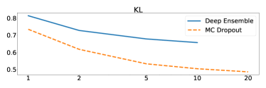
Figure 1: KL divergence of MC Dropout and Deep Ensemble with different numbers of model samples.

6 Results

The performances of different distribution estimation methods are shown in Table 3. The first group (row 2-5) presents the results that do not make use of the soft-labeled data $D^{dev}_{s}$, while the second group (row 6-8) uses $D^{dev}_{s}$. Table 4 shows the performance of distribution estimation methods on the out-of-domain test set and the performance of predicting individual graded plausibility judgments. In what follows, we explain the main findings.

MC Dropout is the most preferable method without additional soft-labeled data.

The first thing we can observe from the first group (row 2-5) in Table 3 is that both MC Dropout and the Deep Ensemble outperform baselines on all the metrics. More importantly, MC Dropout substantially outperforms Deep Ensemble in all KL and JSD columns, with a slight drop on Accuracy. Notice that the MC Dropout results reported in this group are obtained by using the default dropout rate of RoBERTa-Large models (0.1), without tuning on any additional data. The advantage of MC Dropout over Deep Ensemble is different from previous works Lakshminarayanan et al. (2017), and we suspect that this is attributed to the fine-tuning regime of BERT-based models, causing the models in the ensemble to be less diverse. Note that compared to Deep Ensemble, MC dropout does not require training multiple models.

Further improvement can be obtained by using soft-labeled data, but still below estimated human upper-bound.

From the second group (row 6-8) of Table 3, we can see further improvement over the Bayesian methods by using additional 100 soft-labeled data $D^{dev}_{s}$. For example, on ChaosNLI-$\alpha$, Re-Calibration achieves 0.1615 KL (MC Dropout get 0.5045) and 0.1663 JSD (MC Dropout 0.1882). We also include an upper-bound Re-Calibration result by directly applying this method on the test set ($>1000$ examples), but get very close performance to the result with only 100 labels, showing that Re-Calibration is label-efficient. With an additional set of soft-labeled data $D^{dev}_{s}$, we can also tune the optimal dropout rate of MC Dropout. The results are shown in the table with name MC Dropout (Opt. Rate). The JSD and KL performance after tuning are substantially higher than the original MC Dropout, however, there is also a substantial decrease on the overall accuracy, and overall this method does not outperform Re-Calibration. Additionally, Distribution Distillation only gives slightly better JSD than Re-Calibration, with additional computational cost of retraining the model on the whole relabeled training set, indicating that directly applying Re-Calibration is more efficient. Lastly, the best results here are still below estimated human upper-bound, leaving huge room for improvements.

In-domain improvements hold on the out-of-domain set.

Table 4 shows the direct generalization results on PK2019 of the models trained on SNLI and MNLI. All the improvements on the in-domain test sets, including MC Dropout over the baseline and the Re-calibration over the MC Dropout, still hold on the out-of-domain examples in the PK2019 test set. Although the out-of-domain scores are generally lower than the in-domain scores in Table 3, MC Dropout and Re-Calibration can still bring substantial improvements over the baselines without any PK2019 training data.

Correlation exists between opinion distribution and graded individual judgement.

As explained in Sec. 2.3 and 5.1, the distribution of human opinions on NLI examples is different from the individual graded plausibility judgement. In Table 4, we compare the entailment probability output by the distribution estimation method with the graded plausibility scores in UNLI. Although MC dropout and Re-Calibration method under-perform the baseline on Spearman correlation, Re-Calibration can still greatly improve the Pearson correlation $r$. More importantly, our best distribution estimation method without using any UNLI data is noticeably comparable to the reported numbers in UNLI Chen et al. (2020) using a fine-tuned model on in-domain UNLI data. This hints at a certain correlation between opinion distributions and graded individual judgements, consistent with our intuition regarding the interpretation of the labels.

7 Ablation & Analysis

7.1 Ablations for Re-Calibration

In the previous section, we showed the effectiveness of Re-Calibration in predicting human opinion distribution by explicitly utilizing extra soft-labeled data $D^{dev}_{s}$. To get a better sense of what contributes to the performance, we make two ablations on $D^{dev}_{s}$: (1) reducing the size of $D^{dev}_{s}$ from 100 to 10; (2) using only the majority class as hard labels in $D^{dev}_{s}$ rather than the whole label distribution as soft labels for Re-Calibration. Table 5 shows the results. We can observe that with only 10 examples, Re-Calibration can already achieve good performance, with slightly worse KL but slightly better JSD. However, using only the hard labels gives significantly worse scores than using the soft labels on ChaosNLI-M, indicating the necessity of extra annotations in human distribution modeling.

7.2 Sample Sizes in Bayesian Method

In both MC Dropout and Deep Ensemble methods, the distribution is approximated by sampling. To understand how the number of samples will influence the results, we present the result for both methods with different numbers of samples ($k$) on ChaosNLI-$\alpha$ in Figure 1. We can see that while a larger number of samples will lead to better distribution estimation results on KL, the gain is gradually diminished (even with the log-scale x-axis in Figure 1). Similar trends can also be seen on JSD and Accuracy and the figures are in the Appendix D. Considering practical constraints on inference time and computational budget that prohibit a very large number of samples, in our experiments, numbers around 10 is a sweet point between good performance and an acceptable computational budget.

7.3 Distribution Prediction Example

Table 6 shows an example from MNLI with the prediction distribution from both MC Dropout and Re-Calibration. We can see that one-third of humans believe the label should be entailment and two-third as neutral. It is commonsense that clerking for an honorable District Court can be a really rewarding experience, though the premise does not explicitly say so. The MC Dropout method underestimates such a factor and gives more than 80% for the neutral label. Notably, although Re-Calibration method predicts a smoother distribution that resembles human distribution more, it ends up erroneously increasing the probability for the inexplicable contradiction label. Such observation that MC Dropout tends to overlook the disagreement and Re-Calibration can sometimes produce smooth distribution but with erroneously high probabilities is common and should be taken into consideration before practical deployment. More error-analysis examples and a more detailed comparison of the predictions of distribution prediction methods on the whole-dataset level is in the Appendix F, G.

Premise	Professor Rogers began her career by clerking for The Honorable Thomas D. Lambros of the United States District Court for the Northern District of Ohio.
Hypothesis	Her career benefited from being a clerk to Thomas.
Prediction (Entailment / Neutral / Contradiction)
Human Distribution	0.33 / 0.66 / 0.01
MC Dropout	0.1617 / 0.8362 / 0.0021
Re-Calibration	0.3063 / 0.5902 / 0.1035

Table 6: An example of prediction distribution and human ground truth in MNLI.

8 Related Work

Inherent disagreement and ambiguity in NLP annotations has a long history Poesio and Artstein (2005); Zeman (2010) involving tasks like coreference resolution Poesio et al. (2008, 2019); Li et al. (2020), POS-tagging Zeman (2010); Plank et al. (2014, 2016), semantic frame disambiguation Dumitrache et al. (2019), humorousness prediction Simpson et al. (2019), etc. Most previous works design methods to predict one single gold label by aggregating the noisy information Dawid and Skene (1979); Hovy et al. (2013); Rodrigues et al. (2017); Paun et al. (2018); Braylan and Lease (2020); Fornaciari et al. (2021). On the contrary, following the recent definition in NLI works Chen et al. (2020); Pavlick and Kwiatkowski (2019); Nie et al. (2020b), we directly try to predict distribution labels that accurately reflect the opinion of a large population. Peterson et al. (2019) is most similar to us in label definition, and studied the advantage of using distribution labels in image classification.

Uncertainty and calibration have also been studied in various NLP models, from traditional structured prediction models Nguyen and O’Connor (2015), to seq-to-seq models Ott et al. (2018); Kumar and Sarawagi (2019); Xu et al. (2020) and transformers Desai and Durrett (2020). Gantt et al. (2020) suggests a constructive view of NLI modeling in which the prediction is explicitly grounded on annotator identifiers, incorporating the annotator random effects. Zhang and de Marneffe (2021) propose an ensemble-based framework that can identify examples with high label disagreement. Xiao and Wang (2019) shows that explicitly modeling the uncertainty can improve performance, and Wang et al. (2020) propose a label smoothing method that improves calibration for NMT. Instead of aiming for a better uncertainty, our work uses multiple uncertainty estimation methods for more accurate distribution prediction. Concurrently, Meissner et al. (2021) explores training models directly on the multiple labels from each annotator in SNLI and MNLI, Zhang et al. (2021a, b) also leverage distribution labels in the model development process and explore training methods combining the supervision signal of one-hot and distributional labels. In comparison, our work studies additional Bayesian estimation methods and provides a detailed discussion on why and how modeling distribution labels is beneficial for NLU, including the motivation, nuances, and evaluation standardization.

9 Conclusion

We introduce distributed NLI – an extension of NLI with a new goal of predicting human opinion distribution. We show that several distribution estimation methods can capture such distributions more effectively than softmax, but the best results are still far below the estimated upper-bound. We analyze the properties and weaknesses of the methods, highlight the importance of the task, and encourage future work on developing better models for estimating the human opinion distribution.

10 Ethical Considerations

The main target of this paper is to propose a new extension of the NLI task that focuses on predicting the whole distribution instead of one single label. Our new formalization can potentially make the related application of NLI more reliable in the practice, as the models trained on our proposed task will focus more on minority opinions which may be ignored in the traditional formalization. Nonetheless, we are strongly against the use of current NLI models in any critical applications (e.g. admission, jury, etc.). While NLP models can use to help human judgment (and the results should be verified by a human), their robustness and fairness are still an unsolved issue, and cannot replace the work of human experts.

Experiments	Train $D^{train}$	Dev $D^{dev}$	Soft Dev $D^{dev}_{s}$	Test $D^{test}_{s}$
ChaosNLI-$\alpha$	$\alpha$NLItrain (169654)	$\alpha$NLITest (3059)	$\alpha$NLIdev (100)	ChaosNLI-$\alpha$- $D^{dev}_{s}$ (1432)
ChaosNLI-S	SNLItrain + MNLItrain (942854)	SNLITest (10000)	SNLIdev (100)	ChaosNLI-S- $D^{dev}_{s}$ (1414)
ChaosNLI-M	SNLItrain + MNLItrain (942854)	$\text{MNLI}^{\text{dev}}_{\text{mismatch}}$ (10000)	$\text{MNLI}^{\text{dev}}_{\text{match}}$ (100)	ChaosNLI-M- $D^{dev}_{s}$ (1499)
UNLI	-	-	-	UNLI (2998)
PK2019	-	-	-	PK2019 (297)

Table 7: Data sources for each split. The corresponding size of each split is shown in the bracket after the source.

	ChaosNLI-$\alpha$		ChaosNLI-S		ChaosNLI-M
	JSD$\downarrow$	KL$\downarrow$	JSD$\downarrow$	KL$\downarrow$	JSD$\downarrow$	KL$\downarrow$
$D^{dev}_{s}=100$	0.1663	0.1615	0.1889	0.1733	0.2015	0.1873
$D^{dev}_{s}=10$	0.1570	0.1973	0.1744	0.1977	0.1962	0.1940
No soft label	0.1738	0.1630	0.2008	0.3667	0.2347	0.3704

Table 8: Re-calibration performances with different types of labels. $\downarrow$ indicates smaller value is better. $\uparrow$ indicates larger value is better. For each column, the best values are in bold.

Appendix A Dataset Split Details

The details of dataset split, including the source of the data and the corresponding size in Table 7. The UNLI data can be downloaded at https://nlp.jhu.edu/unli/. The PK2019 data is at https://github.com/epavlick/NLI-variation-data. The ChaosNLI data is at https://github.com/easonnie/ChaosNLI.

Appendix B Hyperparameter Details

All the models in this work are built on RoBERTa-Large Liu et al. (2019). For both NLI and $\alpha$NLI tasks, we fine-tune our model with peak learning rate 5e-6, warm-up ratio 0.1 and linear learning rate decay. We use a batch size of 32. We train the NLI model for 2 epochs, and the $\alpha$NLI model for 3 epochs. We always use the accuracy on the development set ($D^{dev}$) for model selection. All our experiments are conducted on a single server with 4 GTX 1080Ti GPUs.

Appendix C Full Re-Calibration Ablation

The full results of Re-Calibration ablations is shown in Table 8. We can see on all three subsets of ChaosNLI, Re-Calibration always achieves good performance even with as few as 10 additional distribution labels; and using 100 distribution labels always significantly outperforms using 100 hard labels without any distribution information.

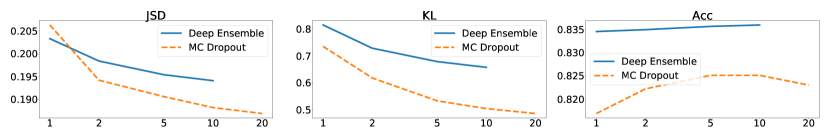
Figure 2: Performances of MC Dropout and Deep Ensemble with different numbers of model samples.

Appendix D The Effect of Sample Size

Figure 2 shows model performances on all three metrics (JSD, KL and Accuracy) with different sample sizes. We can observe similar trends on the KL metric as discussed in the main paper. While a larger number of samples usually leads to better performance, the gain is gradually diminished.

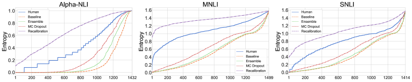
Figure 3: Entropy quantile curve on ChaosNLI. Each point in this figure represents model’s prediction on one example. y-axis is the entropy value, and x-axis is the prediction’s index in a sequence of examples sorted in the increasing-entropy order.

Premise	Hypothesis
Case Description: Some dark night a policeman walks down a street, apparently deserted; but suddenly he hears a burglar alarm, looks across the street, and sees a jewelry store with a broken window. Then a gentleman wearing a mask comes crawling out through the broken window, carrying a bag which turns out to be full of expensive jewelry.	The gentleman is dishonest and guilty for stealing.
The Off Fossil Fuels for a Better Future Act lays out that by 2035: (1) 100% of electricity must be generated from clean energy resources, (2) 100% of vehicle sales from manufacturers must be zero-emission vehicles, and (3) 100% of train rail lines and train engines must be electrified.	Passing the bill means embracing clean energy sources for the good of sustainable development.

Table 9: Examples where AI-aided human decision making can be formulated as an NLI problem.

Appendix E Additional Motivation and Positioning of Distributed NLI

E.1 Potential Applications of Distributed NLI

In order for NLU models to aid humans in decision-making, it is important for NLI models to output a valid distribution and to capture the opinions of the minority sub-populations. We include two example inputs in such situations in Table 9.

Premise	you want to punch the button and go
Hypothesis	You don’t want to push the button lightly, but rather punch it hard.
Prediction (Entailment / Neutral / Contradiction)
Original Annotation	0.48 / 0.45 / 0.07
Incorrect Labels	Contradiction
Reasons for Incorrect Labels	There is no sufficient evidence in the premise indicating "you also want to push the button lightly".
Premise	The tomb guardian will unlock the gate to the tunnel and give you a candle to explore the small circular catacomb, but for what little you can see, it is hardly worth the effort.
Hypothesis	The tomb garden can give you a thorough tour of the catacombs.
Prediction (Entailment / Neutral / Contradiction)
Original Annotation	0.10 / 0.14 / 0.76
Incorrect Labels	Entailment
Reasons for Incorrect Labels	The premise mentions "tomb guardian" instead of "tomb garden", so it should not be entailment.

Table 10: Examples of wrong annotations on the $D^{dev}_{s}$ split of ChaosNLI-M.

Premise	They said that (1) agencies need to be able to design their procedures to fit their particular circumstances (e.g.
Hypothesis	The authors of the recently introduced bill stated each agency would be required to match their operational methods to their particular situations.
Prediction (Entailment / Neutral / Contradiction)
Human Distribution	0.58 / 0.30 / 0.12
Baseline	0.002 / 0.997 / 0.001
Reasons for Ambiguity	Based on different understanding of the phrases "need to be able to" in the premise, this sentence pair can have different labels.
Premise	What changed?
Hypothesis	Nothing changed.
Prediction (Entailment / Neutral / Contradiction)
Human Distribution	0.04 / 0.76 / 0.20
Baseline	0.001 / 0.007 / 0.992
Reasons for Ambiguity	In different contexts, the question in the premise can imply different meanings.

Table 11: Examples of prediction distribution of the baseline model and human ground truth in MNLI.

Model	JSD$\downarrow$		KL$\downarrow$
	Original	Corrected	Original	Corrected
Baseline (Mean)	0.3053	0.3039	0.8383	0.8343
MC Dropout	0.2649	0.2653	0.5851	0.5839
Deep Ensemble	0.2956	0.2941	0.7775	0.7709
Re-Calibration	0.1983	0.2079	0.1859	0.1983

Table 12: Performances difference on the $D^{dev}_{s}$ split of ChaosNLI-M.

E.2 Analysis of Annotation Quality

We manually examined the label correctness of the 100 examples in the $D^{dev}_{s}$ split of ChaosNLI-M. Due to the careful quality control over label collection, only a very limited set of the labels are incorrect. Out of the 100 examples in the examined subset, only 4 examples contain more than 10 error annotations and no example contain more than 16 error annotations. In Table 10, we show two examples of incorrect label annotations in the $D^{dev}_{s}$ split of ChaosNLI-M. While both examples do contain a certain level of semantic ambiguities, with careful reasoning, we do not find sufficient evidence to make the "contradiction" or "entailment" judgement in those cases respectively, hence we view these labels as error annotations.

We also verified these incorrect labels will not substantially impact the results in this paper. For these 100 examples, we removed all the incorrect labels with more than 5 annotations and created a corrected label set. The performance difference between the original annotations and the corrected annotations can be seen in Table 12. We can see only marginal performance difference is shown for the Baseline, MC Dropout and Deep Ensemble variants. The performance difference for the Re-Calibration variant is slighter larger due to the fact that these labels are also directly used in the temperature calibration process, but it also only leads to a relatively small difference around 0.01. Furthermore, using either the original or the corrected labels, the order of more effective methods (Re-Calibration > MC Dropout > Deep Ensemble > Baseline) always holds.

E.3 Predicting Label Distribution from Deterministic Labels

Another question around the feasibility of the Distributed NLI is whether model can learn label distributions if only deterministic labels are possible. Here we prove it is definitely possible if the deterministic labels are annotated by individual annotators. Specifically, if we assume all the training inputs $x$ are randomly sampled from a dataset $D$, and each corresponding label $y$ is provided from a random annotator $a$ from a set of annotators $A$. Then, on the training set, the model is trained to minimize $\displaystyle\mathop{\mathbb{E}}_{x\in D}\mathop{\mathbb{E}}_{a\in A}\textsc{kl}\left(y_{a}(x)\|P(x)\right)$. Specifically, assuming the model parameter is $\theta$, the optimization target is:

$$\operatorname*{arg\,min}_{\theta}\displaystyle\mathop{\mathbb{E}}_{x\in D}\mathop{\mathbb{E}}_{a\in A}\textsc{kl}\left(y_{a}(x)\|P_{\theta}(x)\right)$$

$$= \operatorname*{arg\,min}_{\theta}\displaystyle\mathop{\mathbb{E}}_{x\in D}\mathop{\mathbb{E}}_{a\in A}\sum_{j}y_{a}(x)_{j}\frac{\log y_{a}(x)_{j}}{\log P_{\theta}(x)_{j}}$$

$$= \operatorname*{arg\,min}_{\theta}\displaystyle\mathop{\mathbb{E}}_{x\in D}\mathop{\mathbb{E}}_{a\in A}\sum_{j}-y_{a}(x)_{j}\log P_{\theta}(x)_{j}$$

$$= \operatorname*{arg\,min}_{\theta}\displaystyle\mathop{\mathbb{E}}_{x\in D}\sum_{j}-(\mathop{\mathbb{E}}_{a\in A}y_{a}(x))_{j}\log P_{\theta}(x)_{j}$$

$$= \operatorname*{arg\,min}_{\theta}\displaystyle\mathop{\mathbb{E}}_{x\in D}\sum_{j}(\mathop{\mathbb{E}}_{a\in A}y_{a}(x))_{j}\frac{\log(\mathop{\mathbb{E}}_{a\in A}y_{a}(x))_{j}}{\log P_{\theta}(x)_{j}}$$

$$= \operatorname*{arg\,min}_{\theta}\displaystyle\mathop{\mathbb{E}}_{x\in D}\textsc{kl}\left(\mathop{\mathbb{E}}_{a\in A}y_{a}(x)\|P_{\theta}(x)\right)$$

, where $j$ is each dimension of the output label. Hence, even with deterministic labels, the model still achieves the best performance if and only if when given an example $x$, $P_{\theta}(x)=\displaystyle\mathop{\mathbb{E}}_{a\in A}y_{a}(x)$, where the model correctly predicts the distribution of all labels.

Appendix F More Analysis on Distribution Prediction Examples

In this section, we provided more prediction examples and a more comprehensive analysis in addition to the examples shown in the Ablation & Analysis section in the main paper. Specifically, we focus on analyzing what are the worst-prediction examples produced by current models.

For each model variant, we checked the performance on the $D^{dev}_{s}$ split on ChaosNLI-M and focused on the examples with the largest KL-divergence (worst-prediction examples). For the baseline, we again noticed the trend that models being over-confident on examples with substantial ambiguity. We show two examples in Table 11. In both of these cases, the model fails to capture the label distribution caused by subtle phrase relationships or under-specified meaning depending on the context, etc. As shown in the results section in the main paper, Such over-confidence can be partially alleviated by the Bayesian uncertainty estimation methods (e.g., MC-Dropout and Deep Ensemble) and by the Re-calibration methods. However, most of the top 10 worst-prediction examples of the baseline variant still remain in the top 10 worst-prediction list of the Bayesian and Re-calibration approaches. This observation is possibly due to the limited improvement of Bayesian approaches and the incapability of Re-calibration methods to correct totally wrong predictions, hence showing current models’ inherent incapability to capture these distributions. We also encourage future work to explore the connection between the model’s incapability to capture distribution labels and the model’s tendency to focus on artifact features.

Appendix G Prediction Difference in Bayesian Inference and Re-Calibration

We show that both Bayesian Inference and Re-Calibration can achieve better JSD and KL scores in the main paper. In order to investigate the difference between the predictions produced by the two methods, we conduct the following analysis. Firstly, for each example in the test set, we calculate the entropy for the models outputs as $\mathbf{H}\left(\mathbf{p}\right)=-\sum_{i\in\{e,n,c\}}{p_{i}\log(p_{i})}$ where $p_{i}$ is the probability for entailment, neutral, or contradiction. We also calculate the entropy for human using the annotations in ChaosNLI. We then sort the entropy and plot their entropy values for each model. The plot is shown in Fig. 3. We can see a large gap between the blue line representing human distribution and the orange dashed line representing the baseline, consistent with previous quantitative findings. While Bayesian inference methods can slightly reduce this gap, there is still large room for improvements. Moreover, the distribution predicted by the Re-Calibration method is noticeably different from the ones given by the MC Dropout, Ensemble, and the baseline method, while the latter three are very similar to each other. Finally, it is worth noting that the line for the Re-Calibration method is above the human line while the other three methods are below the human line. This suggests that Re-Calibration method tends to over-predict the disagreement among humans whereas the Bayesian method and the baseline fail to capture some inherent disagreements.

References

- Armour and Sako (2020) John Armour and Mari Sako. 2020. Ai-enabled business models in legal services: from traditional law firms to next-generation law companies? Journal of Professions and Organization, 7(1):27–46.
- Bhagavatula et al. (2020) Chandra Bhagavatula, Ronan Le Bras, Chaitanya Malaviya, Keisuke Sakaguchi, Ari Holtzman, Hannah Rashkin, Doug Downey, Wen-tau Yih, and Yejin Choi. 2020. Abductive commonsense reasoning. In 8th International Conference on Learning Representations, ICLR 2020, Addis Ababa, Ethiopia, April 26-30, 2020. OpenReview.net.
- Bowman et al. (2015) Samuel Bowman, Gabor Angeli, Christopher Potts, and Christopher D Manning. 2015. A large annotated corpus for learning natural language inference. In Proceedings of the 2015 Conference on Empirical Methods in Natural Language Processing, pages 632–642.
- Braylan and Lease (2020) Alexander Braylan and Matthew Lease. 2020. Modeling and aggregation of complex annotations via annotation distances. In Proceedings of The Web Conference 2020, pages 1807–1818.
- Chen et al. (2020) Tongfei Chen, Zhengping Jiang, Adam Poliak, Keisuke Sakaguchi, and Benjamin Van Durme. 2020. Uncertain natural language inference. In Proceedings of the 58th Annual Meeting of the Association for Computational Linguistics, pages 8772–8779, Online. Association for Computational Linguistics.
- Dagan et al. (2005) Ido Dagan, Oren Glickman, and Bernardo Magnini. 2005. The pascal recognising textual entailment challenge. In Machine Learning Challenges Workshop, pages 177–190. Springer.
- Dawid and Skene (1979) Alexander Philip Dawid and Allan M Skene. 1979. Maximum likelihood estimation of observer error-rates using the em algorithm. Journal of the Royal Statistical Society: Series C (Applied Statistics), 28(1):20–28.
- Desai and Durrett (2020) Shrey Desai and Greg Durrett. 2020. Calibration of pre-trained transformers. In Proceedings of the 2020 Conference on Empirical Methods in Natural Language Processing (EMNLP), pages 295–302.
- Dumitrache et al. (2019) Anca Dumitrache, Lora Aroyo, and Chris Welty. 2019. A crowdsourced frame disambiguation corpus with ambiguity. In Proceedings of the 2019 Conference of the North American Chapter of the Association for Computational Linguistics: Human Language Technologies, Volume 1 (Long and Short Papers), pages 2164–2170.
- Eggers et al. (2017) William D. Eggers, David Schatsky, and Peter Viechnicki. 2017. Ai-augmented government using cognitive technologies to redesign public sector work.
- Falke et al. (2019) Tobias Falke, Leonardo F. R. Ribeiro, Prasetya Ajie Utama, Ido Dagan, and Iryna Gurevych. 2019. Ranking generated summaries by correctness: An interesting but challenging application for natural language inference. In Proceedings of the 57th Annual Meeting of the Association for Computational Linguistics, pages 2214–2220, Florence, Italy. Association for Computational Linguistics.
- Fornaciari et al. (2021) Tommaso Fornaciari, Alexandra Uma, Silviu Paun, Barbara Plank, Dirk Hovy, and Massimo Poesio. 2021. Beyond black & white: Leveraging annotator disagreement via soft-label multi-task learning. In Proceedings of the 2021 Conference of the North American Chapter of the Association for Computational Linguistics: Human Language Technologies, Volume 2 (Short Papers).
- Gal (2016) Yarin Gal. 2016. Uncertainty in Deep Learning. Ph.D. thesis, University of Cambridge.
- Gal and Ghahramani (2016) Yarin Gal and Zoubin Ghahramani. 2016. Dropout as a bayesian approximation: Representing model uncertainty in deep learning. In Proceedings of The 33rd International Conference on Machine Learning, volume 48 of Proceedings of Machine Learning Research, pages 1050–1059, New York, New York, USA. PMLR.
- Gantt et al. (2020) William Gantt, Benjamin Kane, and Aaron Steven White. 2020. Natural language inference with mixed effects. In Proceedings of the Ninth Joint Conference on Lexical and Computational Semantics, pages 81–87, Barcelona, Spain (Online). Association for Computational Linguistics.
- Gnanadesikan and Wilk (1968) Ramanathan Gnanadesikan and Martin B Wilk. 1968. Probability plotting methods for the analysis of data. Biometrika, 55(1):1–17.
- Gordon et al. (2021) Mitchell L Gordon, Kaitlyn Zhou, Kayur Patel, Tatsunori Hashimoto, and Michael S Bernstein. 2021. The disagreement deconvolution: Bringing machine learning performance metrics in line with reality. In Proceedings of the 2021 CHI Conference on Human Factors in Computing Systems, pages 1–14.
- Guo et al. (2017) Chuan Guo, Geoff Pleiss, Yu Sun, and Kilian Q Weinberger. 2017. On calibration of modern neural networks. In Proceedings of the 34th International Conference on Machine Learning-Volume 70, pages 1321–1330.
- Hinton et al. (2015) Geoffrey Hinton, Oriol Vinyals, and Jeff Dean. 2015. Distilling the knowledge in a neural network. arXiv preprint arXiv:1503.02531.
- Hovy et al. (2013) Dirk Hovy, Taylor Berg-Kirkpatrick, Ashish Vaswani, and Eduard Hovy. 2013. Learning whom to trust with mace. In Proceedings of the 2013 Conference of the North American Chapter of the Association for Computational Linguistics: Human Language Technologies, pages 1120–1130.
- Jaynes (2003) Edwin T Jaynes. 2003. Probability theory: The logic of science. Cambridge university press.
- Kendall and Gal (2017) Alex Kendall and Yarin Gal. 2017. What uncertainties do we need in bayesian deep learning for computer vision? In Proceedings of the 31st International Conference on Neural Information Processing Systems, pages 5580–5590.
- Kovács et al. (2010) Ágnes Melinda Kovács, Ernő Téglás, and Ansgar Denis Endress. 2010. The social sense: Susceptibility to others’ beliefs in human infants and adults. Science, 330(6012):1830–1834.
- Kumar and Sarawagi (2019) Aviral Kumar and Sunita Sarawagi. 2019. Calibration of encoder decoder models for neural machine translation. arXiv preprint arXiv:1903.00802.
- Lakshminarayanan et al. (2017) Balaji Lakshminarayanan, Alexander Pritzel, and Charles Blundell. 2017. Simple and scalable predictive uncertainty estimation using deep ensembles. In Proceedings of the 31st International Conference on Neural Information Processing Systems, pages 6405–6416.
- Li et al. (2020) Maolin Li, Hiroya Takamura, and Sophia Ananiadou. 2020. A neural model for aggregating coreference annotation in crowdsourcing. In Proceedings of the 28th International Conference on Computational Linguistics, pages 5760–5773.
- Liu et al. (2019) Yinhan Liu, Myle Ott, Naman Goyal, Jingfei Du, Mandar Joshi, Danqi Chen, Omer Levy, Mike Lewis, Luke Zettlemoyer, and Veselin Stoyanov. 2019. Roberta: A robustly optimized bert pretraining approach. arXiv preprint arXiv:1907.11692.
- MacKay (1992) David JC MacKay. 1992. A practical bayesian framework for backpropagation networks. Neural computation, 4(3):448–472.
- Manning (2006) Christopher D. Manning. 2006. Local textual inference: It’s hard to circumscribe.
- Meissner et al. (2021) Johannes Mario Meissner, Napat Thumwanit, Saku Sugawara, and Akiko Aizawa. 2021. Embracing ambiguity: Shifting the training target of NLI models. In Proceedings of the 59th Annual Meeting of the Association for Computational Linguistics and the 11th International Joint Conference on Natural Language Processing (Volume 2: Short Papers), pages 862–869, Online. Association for Computational Linguistics.
- Metropolis and Ulam (1949) Nicholas Metropolis and Stanislaw Ulam. 1949. The monte carlo method. Journal of the American statistical association, 44(247):335–341.
- Neal (1995) Radford M Neal. 1995. BAYESIAN LEARNING FOR NEURAL NETWORKS. Ph.D. thesis, University of Toronto.
- Newman et al. (2020) Grace Newman, Ryan Frazier, and Kandace Miller. 2020. The 2020 recruiting trends report: Covid-19 revision.
- Nguyen and O’Connor (2015) Khanh Nguyen and Brendan O’Connor. 2015. Posterior calibration and exploratory analysis for natural language processing models. In Proceedings of the 2015 Conference on Empirical Methods in Natural Language Processing, pages 1587–1598.
- Nie and Bansal (2017) Yixin Nie and Mohit Bansal. 2017. Shortcut-stacked sentence encoders for multi-domain inference. In Proceedings of the 2nd Workshop on Evaluating Vector Space Representations for NLP, pages 41–45.
- Nie et al. (2020a) Yixin Nie, Adina Williams, Emily Dinan, Mohit Bansal, Jason Weston, and Douwe Kiela. 2020a. Adversarial NLI: A new benchmark for natural language understanding. In Proceedings of the 58th Annual Meeting of the Association for Computational Linguistics. Association for Computational Linguistics.
- Nie et al. (2020b) Yixin Nie, Xiang Zhou, and Mohit Bansal. 2020b. What can we learn from collective human opinions on natural language inference data? In Proceedings of the 2020 Conference on Empirical Methods in Natural Language Processing (EMNLP), pages 9131–9143.
- Ochmann and Laumer (2020) Jessica Ochmann and S. Laumer. 2020. Ai recruitment: Explaining job seekers’ acceptance of automation in human resource management. In Wirtschaftsinformatik.
- Ott et al. (2018) Myle Ott, Michael Auli, David Grangier, and Marc’Aurelio Ranzato. 2018. Analyzing uncertainty in neural machine translation. In International Conference on Machine Learning, pages 3956–3965. PMLR.
- Parikh et al. (2016) Ankur Parikh, Oscar Täckström, Dipanjan Das, and Jakob Uszkoreit. 2016. A decomposable attention model for natural language inference. In Proceedings of the 2016 Conference on Empirical Methods in Natural Language Processing, pages 2249–2255.
- Pasunuru and Bansal (2017) Ramakanth Pasunuru and Mohit Bansal. 2017. Multi-task video captioning with video and entailment generation. In Proceedings of the 55th Annual Meeting of the Association for Computational Linguistics (Volume 1: Long Papers), pages 1273–1283, Vancouver, Canada. Association for Computational Linguistics.
- Paun et al. (2018) Silviu Paun, Jon Chamberlain, Udo Kruschwitz, Juntao Yu, and Massimo Poesio. 2018. A probabilistic annotation model for crowdsourcing coreference. In Proceedings of the 2018 Conference on Empirical Methods in Natural Language Processing, pages 1926–1937.
- Pavlick and Kwiatkowski (2019) Ellie Pavlick and Tom Kwiatkowski. 2019. Inherent disagreements in human textual inferences. Transactions of the Association for Computational Linguistics, 7:677–694.
- Peterson et al. (2019) Joshua C Peterson, Ruairidh M Battleday, Thomas L Griffiths, and Olga Russakovsky. 2019. Human uncertainty makes classification more robust. In Proceedings of the IEEE/CVF International Conference on Computer Vision, pages 9617–9626.
- Plank et al. (2014) Barbara Plank, Dirk Hovy, and Anders Søgaard. 2014. Learning part-of-speech taggers with inter-annotator agreement loss. In Proceedings of the 14th Conference of the European Chapter of the Association for Computational Linguistics, pages 742–751.
- Plank et al. (2016) Barbara Plank, Anders Søgaard, and Yoav Goldberg. 2016. Multilingual part-of-speech tagging with bidirectional long short-term memory models and auxiliary loss. In Proceedings of the 54th Annual Meeting of the Association for Computational Linguistics (Volume 2: Short Papers), pages 412–418.
- Poesio and Artstein (2005) Massimo Poesio and Ron Artstein. 2005. The reliability of anaphoric annotation, reconsidered: Taking ambiguity into account. In Proceedings of the workshop on frontiers in corpus annotations ii: Pie in the sky, pages 76–83.
- Poesio et al. (2019) Massimo Poesio, Jon Chamberlain, Silviu Paun, Juntao Yu, Alexandra Uma, and Udo Kruschwitz. 2019. A crowdsourced corpus of multiple judgments and disagreement on anaphoric interpretation. In Proceedings of the 2019 Conference of the North American Chapter of the Association for Computational Linguistics: Human Language Technologies, Volume 1 (Long and Short Papers), pages 1778–1789.
- Poesio et al. (2008) Massimo Poesio, Uwe Reyle, and Rosemary Stevenson. 2008. Justified sloppiness in anaphoric reference. In Computing meaning, pages 11–31. Springer.
- Poliak et al. (2018) Adam Poliak, Aparajita Haldar, Rachel Rudinger, J Edward Hu, Ellie Pavlick, Aaron Steven White, and Benjamin Van Durme. 2018. Collecting diverse natural language inference problems for sentence representation evaluation. In Proceedings of the 2018 Conference on Empirical Methods in Natural Language Processing.
- Potts et al. (2016) Christopher Potts, Daniel Lassiter, Roger Levy, and Michael C Frank. 2016. Embedded implicatures as pragmatic inferences under compositional lexical uncertainty. Journal of Semantics, 33(4):755–802.
- Ribeiro et al. (2016) Marco Tulio Ribeiro, Sameer Singh, and Carlos Guestrin. 2016. " why should i trust you?" explaining the predictions of any classifier. In Proceedings of the 22nd ACM SIGKDD international conference on knowledge discovery and data mining, pages 1135–1144.
- Rodrigues et al. (2017) Filipe Rodrigues, Mariana Lourenco, Bernardete Ribeiro, and Francisco C Pereira. 2017. Learning supervised topic models for classification and regression from crowds. IEEE transactions on pattern analysis and machine intelligence, 39(12):2409–2422.
- Simpson et al. (2019) Edwin Simpson, Erik-Lân Do Dinh, Tristan Miller, and Iryna Gurevych. 2019. Predicting humorousness and metaphor novelty with gaussian process preference learning. In Proceedings of the 57th Annual Meeting of the Association for Computational Linguistics, pages 5716–5728.
- Socher et al. (2013) Richard Socher, Alex Perelygin, Jean Wu, Jason Chuang, Christopher D Manning, Andrew Y Ng, and Christopher Potts. 2013. Recursive deep models for semantic compositionality over a sentiment treebank. In Proceedings of the 2013 conference on empirical methods in natural language processing, pages 1631–1642.
- Srivastava et al. (2014) Nitish Srivastava, Geoffrey Hinton, Alex Krizhevsky, Ilya Sutskever, and Ruslan Salakhutdinov. 2014. Dropout: a simple way to prevent neural networks from overfitting. The journal of machine learning research, 15(1):1929–1958.
- Surden (2019) Harry Surden. 2019. Artificial intelligence and law: An overview. Georgia State University Law Review, 35:19–22.
- Talmor et al. (2019) Alon Talmor, Jonathan Herzig, Nicholas Lourie, and Jonathan Berant. 2019. CommonsenseQA: A question answering challenge targeting commonsense knowledge. In Proceedings of the 2019 Conference of the North American Chapter of the Association for Computational Linguistics: Human Language Technologies, Volume 1 (Long and Short Papers), pages 4149–4158, Minneapolis, Minnesota. Association for Computational Linguistics.
- Wang et al. (2019) Alex Wang, Amanpreet Singh, Julian Michael, Felix Hill, Omer Levy, and Samuel R. Bowman. 2019. GLUE: A multi-task benchmark and analysis platform for natural language understanding. In 7th International Conference on Learning Representations, ICLR 2019, New Orleans, LA, USA, May 6-9, 2019. OpenReview.net.
- Wang et al. (2020) Shuo Wang, Zhaopeng Tu, Shuming Shi, and Yang Liu. 2020. On the inference calibration of neural machine translation. In Proceedings of the 58th Annual Meeting of the Association for Computational Linguistics, pages 3070–3079.
- Williams et al. (2018) Adina Williams, Nikita Nangia, and Samuel Bowman. 2018. A broad-coverage challenge corpus for sentence understanding through inference. In Proceedings of the 2018 Conference of the North American Chapter of the Association for Computational Linguistics: Human Language Technologies, Volume 1 (Long Papers), pages 1112–1122.
- Xiao and Wang (2019) Yijun Xiao and William Yang Wang. 2019. Quantifying uncertainties in natural language processing tasks. In Proceedings of the AAAI Conference on Artificial Intelligence, volume 33, pages 7322–7329.
- Xu et al. (2020) Jiacheng Xu, Shrey Desai, and Greg Durrett. 2020. Understanding neural abstractive summarization models via uncertainty. In Proceedings of the 2020 Conference on Empirical Methods in Natural Language Processing (EMNLP), pages 6275–6281.
- Zeman (2010) Daniel Zeman. 2010. Hard problems of tagset conversion. In Proceedings of the Second International Conference on Global Interoperability for Language Resources, pages 181–185.
- Zhang et al. (2017) Sheng Zhang, Rachel Rudinger, Kevin Duh, and Benjamin Van Durme. 2017. Ordinal common-sense inference. Transactions of the Association for Computational Linguistics, 5:379–395.
- Zhang et al. (2021a) Shujian Zhang, Chengyue Gong, and Eunsol Choi. 2021a. Capturing label distribution: A case study in nli. arXiv preprint arXiv:2102.06859.
- Zhang et al. (2021b) Shujian Zhang, Chengyue Gong, and Eunsol Choi. 2021b. Learning from uneven training data: Unlabeled, single label, and multiple labels. In Proceedings of the 2021 Conference on Empirical Methods in Natural Language Processing (EMNLP).
- Zhang and de Marneffe (2021) Xinliang Frederick Zhang and Marie-Catherine de Marneffe. 2021. Identifying inherent disagreement in natural language inference. In Proceedings of the 2021 Conference of the North American Chapter of the Association for Computational Linguistics: Human Language Technologies, pages 4908–4915.