“Average” Approximates “First Principal Component”? An Empirical Analysis on Representations from Neural Language Models

Abstract

Contextualized representations based on neural language models have furthered the state of the art in various NLP tasks. Despite its great success, the nature of such representations remains a mystery. In this paper, we present an empirical property of these representations—“average” $\approx$ “first principal component”. Specifically, experiments show that the average of these representations shares almost the same direction as the first principal component of the matrix whose columns are these representations. We believe this explains why the average representation is always a simple yet strong baseline. Our further examinations show that this property also holds in more challenging scenarios, for example, when the representations are from a model right after its random initialization. Therefore, we conjecture that this property is intrinsic to the distribution of representations and not necessarily related to the input structure. We realize that these representations empirically follow a normal distribution for each dimension, and by assuming this is true, we demonstrate that the empirical property can be in fact derived mathematically.

1 Introduction

A large variety of state-of-the-art methods in NLP tasks nowadays are built upon contextualized representations from pre-trained neural language models, such as ELMo Peters et al. (2018), BERT Devlin et al. (2019), and XLNet Yang et al. (2019). Despite the great success, we lack understandings about the nature of such representations. For example, Aharoni and Goldberg (2020) have shown that averaging BERT representations in a sentence can preserve its domain information. However, to our best knowledge, there is no analysis on what leads to the power of averaging representations.

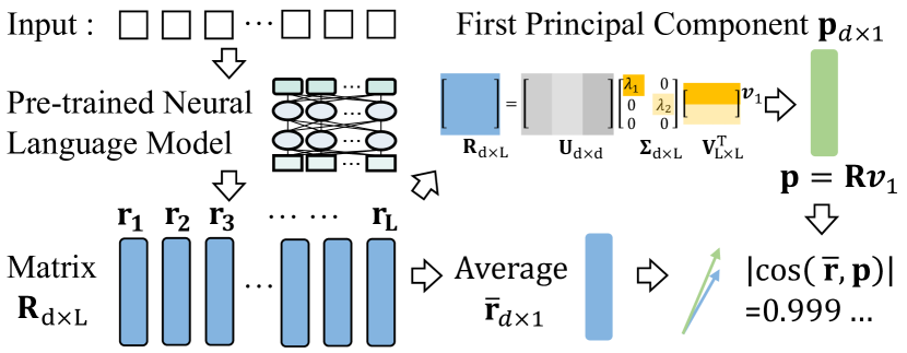
Figure 1: Visualization of our discovered empirical property: “average” $\approx$ “first principal component”.

In this work, we present an empirical property of these representations, “average” $\approx$ “first principal component”. As shown in Figure 1, given a sequence of $L$ tokens, one can construct a $d\times L$ matrix $\mathbf{R}$ using each $d$-dimensional representation $\mathbf{r_{i}}$ of the $i$-th token as a column. There are two popular ways to project this matrix into a single $d$-dimensional vector: (1) average and (2) first principal component. Formally, the average $\overline{\mathbf{r}}$ is a $d$-dimensional vector where $\overline{\mathbf{r}}=\sum_{i=1}^{L}\mathbf{r_{i}}/L$. The first principal component $\mathbf{p}$ is a $d$-dimensional vector whose direction maximizes the variance of the (mean-shifted) $L$ representations. Then, the property can be written as $|\mbox{cos}(\overline{\mathbf{r}},\mathbf{p})|\approx 1$. This absolute value is more than 0.999 in our experiments.

Table 1: Average and minimum absolute cosine similarity of last layer representations between $\overline{\mathbf{r}}$ and $\mathbf{p}$ from 4,000 tests. As a reference, $\mathbf{r_{i}}$ drawn from a uniformly random distribution would lead to Average of .0149.

Model	AG’s news		KP20k		Dbpedia
	Average	Min	Average	Min	Average	Min
BERT	.9994	.9908	.9995	.9958	.9988	.9845
RoBERTa	.9989	.9984	.9990	.9982	.9987	.9980
XLNet	.9990	.9874	.9991	.9932	.9994	.9856
ELMo	.9957	.9681	.9985	.9666	.9949	.9355
Word2vec	.9590	.8506	.9647	.8907	.9530	.8474
Glove	.9639	.5014	.9839	.6369	.9697	.6088

Table 2: Average and minimum absolute cosine similarity between $\overline{\mathbf{r}}$ and $\mathbf{p}$ from 4,000 tests from AG’s news.

Model	Same Sentence		Random Sentence
	Average	Min	Average	Min
BERT	.9994	.9908	.9992	.9930
RoBERTa	.9989	.9984	.9989	.9985
XLNet	.9990	.9874	.9994	.9960
ELMo	.9957	.9681	.9860	.6836
Word2vec	.9590	.8506	.9405	.8497
Glove	.9639	.5014	.9546	.3102

We examine the generality of this property and find it also holds in three more scenarios when every $\mathbf{r_{i}}$ is drawn from (1) a fixed layer (not necessary the last layer) in a pre-trained neural language model, (2) a fixed layer in a model right after random initialization without any training, and (3) random token representations from all sentences encoded by a pre-trained model. Therefore, we conjecture that this property is intrinsic to the representations’ distribution, which is related to the neural language model’s architecture and parameters, and not necessarily related to the input structure. We realize that the empirical distribution of these representations is similar to a normal distribution on each dimension. Assuming this is true, we show that the property can be in fact derived mathematically.

Our contributions are summarized as follow.

• We discover a common, insightful property of several pre-trained neural language models—“average” $\approx$ “first principal component”. To some extent, this explains why the average representation is always a simple yet strong baseline.

• We verify the generality of this property by obtaining representations from a random mixture of layers and sentences and also using randomly initialized models instead of pre-trained ones.

• We show that representations from language models empirically follow a per-dimension normal distribution that leads to the property.

Reproducibility. We will release code to reproduce experiments on Github.

2 Experimental Settings

Dataset. We random sample 4,000 sentences each from three different datasets on three different domains: AG’s news corpus Zhang et al. (2015), KP20k Computer Science papers Meng et al. (2017), and DBpedia Zhang et al. (2015).

Pre-trained Neural Language Models. We experiment on four well-known language models: (1) BERT Devlin et al. (2019), (2) RoBERTa Liu et al. (2019), (3) XLNet Yang et al. (2019), and (4) ELMo Peters et al. (2018). For the first four transformer-based models, we use the base (and cased, if available) version from the HuggingFace’s Wolf et al. (2019) implementation. For ELMo, we follow the AllenNLP toolbox Gardner et al. (2018).

Word Embedding Models. We include experiments on word embeddings Word2vec Mikolov et al. (2013) and Glove Pennington et al. (2014) learned on Wikipedia Fares et al. (2017).

3 The Property: “Average” $\approx$ “First Principal Component”

In most applications, each representation $\mathbf{r_{i}}$ in $\mathbf{R}$ comes from the tokens within the Same Sentence and the last layer of a pre-trained neural language model. Following this setting, we conduct 4,000 tests each on three datasets and summarize the results in Table 1. One can easily see that the average and min absolute cosine similarities are very close to 1 for all pre-trained neural language models. The word embeddings satisfy the property on average, but not for some outlier sentences . Given that uniformly random representations have near-zero average and min absolute cosine similarity values, we conclude that this is a special property for the language model generated representations. To some extent, it explains the effectiveness of the average last-layer representation based on a language model, which has been widely adopted and observed in the literature.

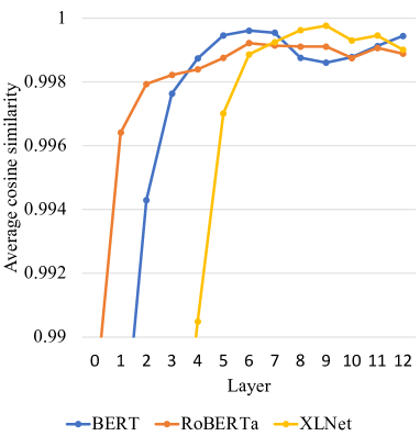
(a) Pre-trained

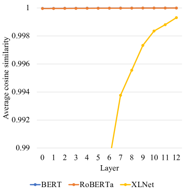
(b) Randomly Initialized

Figure 2: Average cosine similarity for different layers.

4 Generality Tests of the Property

Different Layers. To evaluate our discovered property’s generality, we first investigate if this property only holds for the last-layer representations. For the four transformer-based language models, there are 13 possible layers (i.e., one after lookup table and 12 after encoder/decoder layers) to retrieve representations for tokens. Therefore, we test the property based on representations from each layer and plot the average absolute cosine similarities in Figure 2. One can see that the property holds for the last few layers in all four models.

Random Initialized Models. We repeat the same test for randomly initialized models, i.e., not (pre-)trained at all. The results are in Figure 2. Again, we can see that the property holds for the last few layers in all four models.

Random Sentence. Finally, we explore the case when the representations can even come from different sentences. Specifically, we shuffle all the last-layer token representations of the 4,000 sentences and re-group them into 4,000 random lists of representations. With a high probability, each token representation in a list is generated independently of other tokens from the same list. We show the results in Random Sentences section in Table 2. Surprisingly, even with “unrelated” token representations, the property still holds well.

5 Analysis

In this section, we attempt to answer what could be a reason that the language models show this property. From Section 4, we know that the property also holds for randomly initialized models. Such models know nothing about natural languages. Therefore, it is reasonable to believe that this property is intrinsic to the models and related to the distribution of these representations.

5.1 Representation Distribution Analysis: BERT as a Case Study

We show that each dimension of BERT representations likely follows a normal distribution.

From Figure 3, we can see that the quantiles match with a normal distribution almost perfectly through a Q-Q plot Wilk and Gnanadesikan (1968) on the first dimension. We have checked another ten random dimensions and their quantiles all match well (see Appendix).

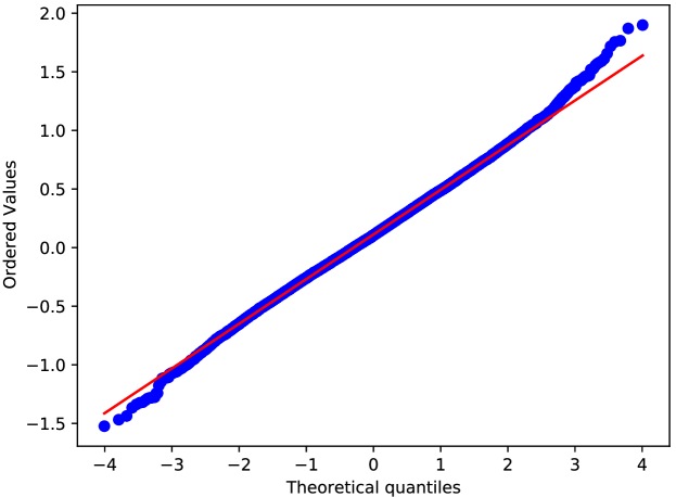
Figure 3: Q-Q plot of the 1st dimension of BERT representations against a normal distribution. We sampled 10% of representations to reduce the figure size.

We also compare the skewness and kurtosis of a standard normal distribution and the empirical distribution of standardized representation values in each dimension. Let $\mathbf{s_{j}}$ be the vector that contains values of dimension $j$ in the representations. Specifically, consider the representation matrix $\mathbf{R^{\prime}}$ for all $D=224,970$ representations over the 4,000 sentences. The rows of $\mathbf{R^{\prime}}$ correspond to $\mathbf{s_{j}}$. The standardized vector $\widetilde{\mathbf{s_{j}}}$ of $\mathbf{s_{j}}$ is defined as $\widetilde{s_{ji}}=\frac{s_{ji}-\hat{\mu}_{j}}{\hat{\sigma}_{j}}$, where $\hat{\mu}_{j}=\frac{\sum_{i=1}^{D}s_{ji}}{D}$ and $\hat{\sigma_{j}}=\sqrt{\frac{\sum_{i=1}^{D}(s_{ji}-\hat{\mu}_{j})^{2}}{D}}$. For each dimension $j,1\leq j\leq d$, one can obtain an empirical distribution from $\widetilde{\mathbf{s_{j}}}$. From Table 3, the third moment matches with a standard normal distribution well, while the fourth moment is a bit off. Further, we examine the the off diagonal terms in the $d\times d$ covariance matrix of the representations, which has a mean of 0.0101 and a standard deviation of 0.0116. When compared with a mean of 0.1747 of the diagonal terms, this is very small. Therefore, we conjecture that each dimension of BERT’s representation can be treated approximately like an independent normal distribution. We note that we do not perform normality tests due to the large dataset size (i.e., over 200,000 representations), since even a minor shift away from the normal distribution can make statistical tests reject the null hypothesis.

Table 3: $N(0,1)$ vs. the Distribution of Normalized BERT Representations. For empirical values, we show Avg($\pm$Std) over 768 dimensions.

	$\sim N(0,1)$	$\sim\mbox{Distribution}(\widetilde{\mathbf{s_{j}}}$)
Skewness ($\mathbb{E}[z^{3}]$)	0	0.0062($\pm{0.5884}$)
Kurtosis ($\mathbb{E}[z^{4}]$)	3	3.9629($\pm{3.3821}$)

In the rest of this section, we assume representations are sampled from $d$ normal distributions, i.e., each dimension follows a distribution $N(\mu_{j},\sigma_{j}^{2})$.

5.2 Fitted distributions satisfy the property

Table 4: Property testing results of representations following $d$ normal distributions with $\mu_{j}$ and $\sigma_{j}$ sampled from certain uniform distributions. 4000 tests are done.

$r_{ij}\sim N(\mu_{j},\sigma_{j}^{2})$	Average	Min
$\mu_{j}\sim\mathcal{U}[-1,1],\sigma_{j}\sim\mathcal{U}[0,1]$	.9986	.9939
$\mu_{j}\sim\mathcal{U}[-1,1],\sigma_{j}\sim\mathcal{U}[0,10]$	.1475	.0000
$\mu_{j}\sim\mathcal{U}[3,5],\sigma_{j}\sim\mathcal{U}[0,1]$	.1490	.1463
$\mu_{j}=0,\sigma_{j}\sim\mathcal{U}[0,1]$	.1587	.0000

We verify the property on generated representations following the distribution. When the parameters $\mu_{j},\sigma_{j}$ are estimated from representations from language models, the property holds (see Appendix). We can also randomly sample the parameters from pre-defined distributions, as shown in Table 4. The results on pre-defined distributions tell us: (1) the average of all $\mu_{j}$ should be 0, (2) not all of $\mu_{j}$ should be exactly 0, and (3) the variance should not be too large in magnitude compared to the mean.

In the following analysis, we additionally restrict that all representations have a sum of value to 0, i.e. $\sum_{j=1}^{d}r_{ij}=0,$ for all representations $\mathbf{r_{i}}$. This is mainly for the simplicity of the covariance matrix computation, as the PCA algorithm will first mean-shift the R matrix.

5.3 Covariance Matrix $\mathbf{C}$ of Normally Distributed Representations

We define the L-by-L covariance matrix $\mathbf{C}=\mathbf{R}^{\intercal}\mathbf{R}$. Its L-by-1 eigenvector $\mathbf{w}$ corresponding to the largest eigenvalue can be used to get the first principal component, i.e., $\mathbf{p}=\mathbf{R}\mathbf{w}$.

We show that if the representations follow a per-dimension normal distribution, $\mathbf{C}$ will follow a special shape—by expectation, its diagonals and off-diagonals will be the same positive value, respectively. We theoretically derive the mean and standard deviation of the entries based on $\mu_{j}$ and $\sigma_{j}$ (derivations are available in Appendix), empirically estimate their values, and put them in Table 5. It is clear that the standard deviation is smaller than the mean in magnitudes, confirming the special shape of $\mathbf{C}$. Also, the theoretical and estimated values mostly match. The only significant difference is the standard deviation for diagonal entries, which is due to the difference on the fourth power statistics between the representations and the standard normal distribution as shown in Table 3.

5.4 This Special $\mathbf{C}$ $\rightarrow$ the Property

If the diagonal entries of the covariance matrix $\mathbf{C}$ are $a>0$, and all off-diagonal entries are $b>0$, the eigenvector $\mathbf{w}$ corresponding to the largest eigenvalue will be a uniform vector. The Perron–Frobenius theorem Samelson (1957) states that the (unique) largest eigenvalue $\lambda$ is bounded:

$$\min_{i}\sum_{j=1}^{L}C_{ij}\leq\lambda\leq\max_{i}\sum_{j=1}^{L}C_{ij},$$ (1)

which refer to the min and max row-sums in $\mathbf{C}$. Due to its special shape, all row-sums in $\mathbf{C}$ are around $a+b*(L-1)$. Therefore, the largest eigenvalue $\lambda_{1}\approx a+b*(L-1)$. To obtain $\mathbf{w}$, one can solve $\mathbf{C}\mathbf{w}=\lambda_{1}\mathbf{w}$. Obviously, $\mathbf{w}=\mathbf{1}$ is a solution, where $\mathbf{1}$ is a vector of 1’s of length $L$. As a result, the first principal component $\mathbf{p}=\mathbf{R}\mathbf{w}$ follows the same direction as the average.

Table 5: Theoretical and Estimated Mean and Standard Deviation of the Values in the Covariance Matrix $\mathbf{C}$.

	Theoretical		Estimated
	Mean	Std	Mean	Std
diagonal	0.2857	0.0350	0.2857	0.0710
off-diagonal	0.1100	0.0248	0.1100	0.0248

6 Related Work

Simply averaging is a widely used, strong baseline to aggregate (contextualized) token representations Ethayarajh (2019); Aharoni and Goldberg (2020); Reimers and Gurevych (2019); Zhang et al. (2015); Taddy (2015); Yu et al. (2018). In this paper, we discover an empirical property of these representations (“average” $\approx$ “first principal component”), which can justify its effectiveness.

There are other attempts to analyze properties of language models. Clark et al. (2019) analyze syntactic information that BERT’s attention maps capture. K et al. (2020) prune the causes for multilinguality of multilingual BERT. Wang and Chen (2020) show that position information are learned differently in different language models. Different from these language-specific properties, we believe our newly discovered property relates more to the internal structure of neural language models.

7 Conclusion and Future Work

This paper shows a common, insightful property of representations from neural language models—“average” $\approx$ “first principal component”. This property is general and holds in many challenging scenarios. After analyzing the BERT representations as a case study, we conjecture that these representations follow a normal distribution for each dimension, and this distribution leads to our discovered property. We believe that this work can shed light on future directions: (1) identifying the distributions that representations from language models follow, and (2) further implications or properties that representations have.

Appendix A Q-Q Plot of Ten Random Dimensions

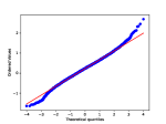
(a) d = 29

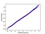
(b) d = 94

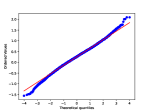
(c) d = 287

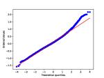
(d) d = 342

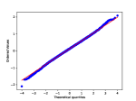
(e) d = 390

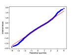
(f) d = 495

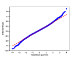
(g) d = 507

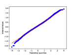
(h) d = 527

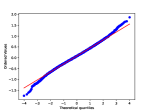
(i) d = 655

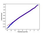
(j) d = 670

Figure 4: Q-Q plots on ten random dimensions.

We randomly sample another 10 dimensions from the 768 dimensions of BERT and plot the quantiles against a normal distribution in Figure 4. All the 10 dimensions match with a normal distribution pretty well.

Table 6: Representations following $d$ normal distributions with parameters estimated from neural language models.

Model	Average	Min
BERT	.9995	.9978
RoBERTa	.9989	.9982
GPT-2	.9988	.9982
XLNet	.9994	.9977
ELMo	.9987	.9947

Appendix B Normal Distribution Estimated from Models

In additional to randomly sampled $\mu_{j}$ and $\sigma_{j}$, we can also use the empirical mean and standard deviation of (dimensions of) representations from pre-trained language models. Table 6 shows that the property is well satisfied on these representations. This further advocates that representations from these models have properties similar to normal distributions.

Appendix C Diagonal & Off-diagonal Values

Here we show the calculations for values in the covariance matrix $C$. Note that

$$C_{ij}=\frac{1}{d-1}\sum_{k=1}^{d}r_{ki}r_{kj},$$

so for diagonal entries $C_{ii}$ is a sum of $d$ products of normally distributed random variables with itself, and all $C_{ii}$ follow the same distribution; for off diagonal entries $C_{ij}$ is a sum of $d$ products of pairs of normally distributed random variables, and similarly, all off diagonal entries also follow the same distribution. Therefore, on expectation, the covariance matrix have the same diagonal entries, and the same off-diagonal entries. The average and variance can be mathematically derived:

$$\begin{split}\mathbb{E}[C_{ii}]&=\frac{1}{d-1}\sum_{k=1}^{d}(\sigma_{k}^{2}+\mu_{k}^{2})\\ Var[C_{ii}]&=\frac{1}{(d-1)^{2}}\left(\sum_{k=1}^{d}2\sigma_{k}^{4}+4\mu_{k}^{2}\sigma_{k}^{2}\right)\\ \mathbb{E}[C_{ij}]&=\frac{1}{d-1}\sum_{k=1}^{d}\mu_{k}^{2}\\ Var[C_{ij}]&=\frac{1}{(d-1)^{2}}\left(\sum_{k=1}^{d}\sigma_{k}^{4}+2\mu_{k}^{2}\sigma_{k}^{2}\right)\end{split}$$

We also outline steps for the derivation. Following our notations, $r_{ij}\sim N(\mu_{j},\sigma_{j}^{2})\implies r_{ij}=\sigma_{j}*z_{ij}+\mu_{j}$ where $z_{ij}$ is a standard normal variable, i.e. $z_{ij}\sim N(0,1)$.

$$\begin{split}E[C_{ii}]&=E[\frac{1}{d-1}*\sum_{k=1}^{d}r_{ik}r_{ik}]\\ &=\frac{1}{d-1}\sum_{k=1}^{d}E[(\sigma_{k}*z_{ik}+\mu_{k})^{2}]\\ &=\frac{1}{d-1}\sum_{k=1}^{d}(\sigma_{k}^{2}+\mu_{k}^{2})\end{split}$$ (2)

$$\begin{split}E[C_{ij}]&=E[\frac{1}{d-1}*\sum_{k=1}^{d}r_{ik}r_{jk}]\\ &=\frac{1}{d-1}\sum_{k=1}^{d}E[(\sigma_{k}*z_{ik}+\mu_{k})(\sigma_{k}*z_{jk}+\mu_{k})]\\ &=\frac{1}{d-1}\sum_{k=1}^{d}(\mu_{k}^{2})\end{split}$$ (3)

$$\begin{split}Var[C_{ii}]&=E[\left(\frac{1}{d-1}*\sum_{k=1}^{d}r_{ki}r_{ki}\right)^{2}]-E[C_{ii}]^{2}\\ &=\frac{1}{(d-1)^{2}}E[(\sum_{k=1}^{d}r_{ki}*r_{ki})^{2}]-E[C_{ii}]^{2}\end{split}$$ (4)

$$\begin{split}E[(\sum_{k=1}^{d}r_{ki}*r_{ki})^{2}]&=E[(\sum_{k=1}^{d}(\sigma_{k}z_{ik}+\mu_{k})^{2})^{2}]\\ &=\sum_{k=1}^{d}E[(\sigma_{k}^{2}z_{ik}^{2}+2\mu_{k}\sigma_{k}z_{ik}+\mu_{k}^{2})^{2}]\\ &\textrm{\;\;\;\;}+\sum_{k_{1}!=k_{2}}E[(\sigma_{k_{1}}^{2}z_{i{k_{1}}}^{2}+2\mu_{k_{1}}\sigma_{k_{1}}z_{i{k_{1}}}+\mu_{k_{1}}^{2})*(\sigma_{k_{2}}^{2}z_{i{k_{2}}}^{2}+2\mu_{k_{2}}\sigma_{k_{2}}z_{i{k_{2}}}+\mu_{k_{2}}^{2})]\\ &=\sum_{k=1}^{d}E[(\sigma_{k}^{2}z_{ik}^{2}+\mu_{k}^{2})^{2}+4\mu_{k}^{2}\sigma_{k}^{2}z_{ik}^{2}]+\sum_{k_{1}!=k_{2}}(\sigma_{k_{1}}^{2}+\mu_{k_{1}}^{2})*(\sigma_{k_{2}}^{2}+\mu_{k_{2}}^{2})\\ &=\sum_{k=1}^{d}\sigma_{k}^{4}*3+\mu_{k}^{4}+2*\sigma_{k}^{2}\mu_{k}^{2}+4\mu_{k}^{2}\sigma_{k}^{2}+\sum_{k_{1}!=k_{2}}(\sigma_{k_{1}}^{2}+\mu_{k_{1}}^{2})*(\sigma_{k_{2}}^{2}+\mu_{k_{2}}^{2})\\ &=\left(\sum_{k=1}^{d}\sigma_{k}^{2}+\mu_{k}^{2}\right)^{2}+\sum_{k=1}^{d}2\sigma_{k}^{4}+4\mu_{k}^{2}\sigma_{k}^{2}\end{split}$$ (5)

$$\begin{split}Var[C_{ij}]&=E[\left(\frac{1}{d-1}*\sum_{k=1}^{d}r_{ki}r_{kj}\right)^{2}]-E[C_{ij}]^{2}\\ &=\frac{1}{(d-1)^{2}}E[(\sum_{k=1}^{d}r_{ki}*r_{kj})^{2}]-E[C_{ij}]^{2}\end{split}$$ (6)

$$\begin{split}E[(\sum_{k=1}^{d}r_{ki}*r_{kj})^{2}]&=E[\left(\sum_{k=1}^{d}(\sigma_{k}z_{ik}+\mu_{k})*(\sigma_{k}z_{jk}+\mu_{k})\right)^{2}]\\ &=\sum_{k=1}^{d}E[(\sigma_{k}^{2}z_{ik}z_{jk}+\mu_{k}\sigma_{k}(z_{ik}+z_{jk})+\mu_{k}^{2})^{2}]\\ &\;\;+\sum_{k_{1}!=k_{2}}E[(\sigma_{k_{1}}^{2}z_{i{k_{1}}}z_{j{k_{1}}}+\mu_{k_{1}}\sigma_{k_{1}}(z_{i{k_{1}}}+z_{j{k_{1}}})+\mu_{k_{1}}^{2})\\ &\;\;*(\sigma_{k_{2}}^{2}z_{i{k_{2}}}z_{j{k_{2}}}+\mu_{k_{2}}\sigma_{k_{2}}(z_{i{k_{2}}}+z_{j{k_{2}}})+\mu_{k_{2}}^{2})]\\ &=\sum_{k=1}^{d}E[(\sigma_{k}^{2}z_{ik}z_{jk}+\mu_{k}^{2})^{2}+\mu_{k}^{2}\sigma_{k}^{2}(z_{ik}+z_{jk})^{2}]+\sum_{k_{1}!=k_{2}}\mu_{k_{1}}^{2}*\mu_{k_{2}}^{2}\\ &=\sum_{k=1}^{d}\sigma_{k}^{4}+\mu_{k}^{4}+\mu_{k}^{2}\sigma_{k}^{2}*2+\sum_{k_{1}!=k_{2}}\mu_{k_{1}}^{2}*\mu_{k_{2}}^{2}\\ &=\left(\sum_{k=1}^{d}\mu_{k}^{2}\right)^{2}+\sum_{k=1}^{d}\sigma_{k}^{4}+2\mu_{k}^{2}\sigma_{k}^{2}\end{split}$$ (7)

References

- Aharoni and Goldberg (2020) Roee Aharoni and Yoav Goldberg. 2020. Unsupervised domain clusters in pretrained language models. In Proceedings of the 58th Annual Meeting of the Association for Computational Linguistics, ACL 2020, Online, July 5-10, 2020, pages 7747–7763. Association for Computational Linguistics.
- Clark et al. (2019) Kevin Clark, Urvashi Khandelwal, Omer Levy, and Christopher D. Manning. 2019. What does BERT look at? an analysis of bert’s attention. CoRR, abs/1906.04341.
- Devlin et al. (2019) Jacob Devlin, Ming-Wei Chang, Kenton Lee, and Kristina Toutanova. 2019. BERT: pre-training of deep bidirectional transformers for language understanding. In Proceedings of the 2019 Conference of the North American Chapter of the Association for Computational Linguistics: Human Language Technologies, NAACL-HLT 2019, Minneapolis, MN, USA, June 2-7, 2019, Volume 1 (Long and Short Papers), pages 4171–4186. Association for Computational Linguistics.
- Ethayarajh (2019) Kawin Ethayarajh. 2019. How contextual are contextualized word representations? comparing the geometry of bert, elmo, and GPT-2 embeddings. In Proceedings of the 2019 Conference on Empirical Methods in Natural Language Processing and the 9th International Joint Conference on Natural Language Processing, EMNLP-IJCNLP 2019, Hong Kong, China, November 3-7, 2019, pages 55–65. Association for Computational Linguistics.
- Fares et al. (2017) Murhaf Fares, Andrey Kutuzov, Stephan Oepen, and Erik Velldal. 2017. Word vectors, reuse, and replicability: Towards a community repository of large-text resources. In Proceedings of the 21st Nordic Conference on Computational Linguistics, NODALIDA 2017, Gothenburg, Sweden, May 22-24, 2017, volume 131 of Linköping Electronic Conference Proceedings, pages 271–276. Linköping University Electronic Press / Association for Computational Linguistics.
- Gardner et al. (2018) Matt Gardner, Joel Grus, Mark Neumann, Oyvind Tafjord, Pradeep Dasigi, Nelson F. Liu, Matthew E. Peters, Michael Schmitz, and Luke Zettlemoyer. 2018. Allennlp: A deep semantic natural language processing platform. CoRR, abs/1803.07640.
- K et al. (2020) Karthikeyan K, Zihan Wang, Stephen Mayhew, and Dan Roth. 2020. Cross-lingual ability of multilingual BERT: an empirical study. In 8th International Conference on Learning Representations, ICLR 2020, Addis Ababa, Ethiopia, April 26-30, 2020. OpenReview.net.
- Liu et al. (2019) Yinhan Liu, Myle Ott, Naman Goyal, Jingfei Du, Mandar Joshi, Danqi Chen, Omer Levy, Mike Lewis, Luke Zettlemoyer, and Veselin Stoyanov. 2019. Roberta: A robustly optimized BERT pretraining approach. CoRR, abs/1907.11692.
- Meng et al. (2017) Rui Meng, Sanqiang Zhao, Shuguang Han, Daqing He, Peter Brusilovsky, and Yu Chi. 2017. Deep keyphrase generation. In Proceedings of the 55th Annual Meeting of the Association for Computational Linguistics, ACL 2017, Vancouver, Canada, July 30 - August 4, Volume 1: Long Papers, pages 582–592. Association for Computational Linguistics.
- Mikolov et al. (2013) Tomas Mikolov, Ilya Sutskever, Kai Chen, Gregory S. Corrado, and Jeffrey Dean. 2013. Distributed representations of words and phrases and their compositionality. In Advances in Neural Information Processing Systems 26: 27th Annual Conference on Neural Information Processing Systems 2013. Proceedings of a meeting held December 5-8, 2013, Lake Tahoe, Nevada, United States, pages 3111–3119.
- Pennington et al. (2014) Jeffrey Pennington, Richard Socher, and Christopher D. Manning. 2014. Glove: Global vectors for word representation. In Proceedings of the 2014 Conference on Empirical Methods in Natural Language Processing, EMNLP 2014, October 25-29, 2014, Doha, Qatar, A meeting of SIGDAT, a Special Interest Group of the ACL, pages 1532–1543. ACL.
- Peters et al. (2018) Matthew E. Peters, Mark Neumann, Mohit Iyyer, Matt Gardner, Christopher Clark, Kenton Lee, and Luke Zettlemoyer. 2018. Deep contextualized word representations. In Proceedings of the 2018 Conference of the North American Chapter of the Association for Computational Linguistics: Human Language Technologies, NAACL-HLT 2018, New Orleans, Louisiana, USA, June 1-6, 2018, Volume 1 (Long Papers), pages 2227–2237. Association for Computational Linguistics.
- Reimers and Gurevych (2019) Nils Reimers and Iryna Gurevych. 2019. Sentence-bert: Sentence embeddings using siamese bert-networks. In Proceedings of the 2019 Conference on Empirical Methods in Natural Language Processing and the 9th International Joint Conference on Natural Language Processing, EMNLP-IJCNLP 2019, Hong Kong, China, November 3-7, 2019, pages 3980–3990. Association for Computational Linguistics.
- Samelson (1957) Hans Samelson. 1957. On the perron-frobenius theorem. Michigan Math. J., 4(1):57–59.
- Taddy (2015) Matt Taddy. 2015. Document classification by inversion of distributed language representations. In Proceedings of the 53rd Annual Meeting of the Association for Computational Linguistics and the 7th International Joint Conference on Natural Language Processing of the Asian Federation of Natural Language Processing, ACL 2015, July 26-31, 2015, Beijing, China, Volume 2: Short Papers, pages 45–49. The Association for Computer Linguistics.
- Wang and Chen (2020) Yu-An Wang and Yun-Nung Chen. 2020. What do position embeddings learn? an empirical study of pre-trained language model positional encoding. In Proceedings of the 2020 Conference on Empirical Methods in Natural Language Processing, EMNLP 2020, Online, November 16-20, 2020, pages 6840–6849. Association for Computational Linguistics.
- Wilk and Gnanadesikan (1968) M. B. Wilk and R. Gnanadesikan. 1968. Probability plotting methods for the analysis of data. Biometrika, 55(1):1–17.
- Wolf et al. (2019) Thomas Wolf, Lysandre Debut, Victor Sanh, Julien Chaumond, Clement Delangue, Anthony Moi, Pierric Cistac, Tim Rault, Rémi Louf, Morgan Funtowicz, and Jamie Brew. 2019. Huggingface’s transformers: State-of-the-art natural language processing. CoRR, abs/1910.03771.
- Yang et al. (2019) Zhilin Yang, Zihang Dai, Yiming Yang, Jaime G. Carbonell, Ruslan Salakhutdinov, and Quoc V. Le. 2019. Xlnet: Generalized autoregressive pretraining for language understanding. In Advances in Neural Information Processing Systems 32: Annual Conference on Neural Information Processing Systems 2019, NeurIPS 2019, 8-14 December 2019, Vancouver, BC, Canada, pages 5754–5764.
- Yu et al. (2018) Katherine Yu, Haoran Li, and Barlas Oguz. 2018. Multilingual seq2seq training with similarity loss for cross-lingual document classification. In Proceedings of The Third Workshop on Representation Learning for NLP, Rep4NLP@ACL 2018, Melbourne, Australia, July 20, 2018, pages 175–179. Association for Computational Linguistics.
- Zhang et al. (2015) Xiang Zhang, Junbo Jake Zhao, and Yann LeCun. 2015. Character-level convolutional networks for text classification. In Advances in Neural Information Processing Systems 28: Annual Conference on Neural Information Processing Systems 2015, December 7-12, 2015, Montreal, Quebec, Canada, pages 649–657.