Observations of AR Sco with $Chandra$ and AstroSat Soft X-ray Telescope

Abstract

We present our AstroSat soft X-ray observations of a compact binary system, AR Sco, and analysis of its X-ray observations with $Chandra$ that were taken only about a week before the AstroSat observations. An analysis of the soft X-ray ($0.3-2.0$ keV) data limits the modulation of the spin, orbital, or beat periods to less than 0.03 counts s^-1 or $<$10% of the average count rate. The X-ray flux obtained from both observatories is found to be almost identical (within a few percent) in flux, and about 30% lower than reported from the nine months older observations with XMM-Newton. A two-temperature thermal plasma model with the same spectral parameters fit $Chandra$ and AstroSat data very well, and requires very little absorption in the line of sight to the source. The low-temperature component has the same temperature ($\sim$1 keV) as reported earlier, but the high-temperature component has a lower temperature of 5.0${}^{+0.8}_{-0.7}$ keV as compared to 8.0 keV measured earlier, however, the difference is not statistically significant.

kpsinghx52@gmail.com

xxxxxxxx

12.3456/s78910-011-012-3 #### 000 0000 1– 1

1 Introduction

A uniquely variable star, AR Scorpii (AR Sco) was initially mis-classified as a pulsating $\delta$-Scuti type (Satyvaldiev, V. 1971). The star is at a distance of 117$\pm$1 pc based on parallax measurements given in Gaia Early Data Release 3 by Gaia Collaboration, Brown et al. (2020), with statistical error as given at the Gaia website. It gained prominence when it was identified as a rare radio pulsing white dwarf (WD) binary system by Marsh et al. (2016). A very short spin period of P_s=117.1 s, and a synodic (spin$-$orbital beat) period, P_b=118.2 s and its harmonics, with very high amplitudes of P_b in the ultraviolet, optical and infra-red were found by Marsh et al. (2016). These periods were also seen at radio frequencies, and a slowing of the synodic period ($\dot{\rm P}_{b}$=3.92$\times$10^-13s s^-1) was also reported by Marsh et al (2016), thus implying a time-scale of 10⁷ years for synchronization. However, in more recent photometric studies by Stiller et al. (2018) and Gaibor et al. (2020), the latter from data taken over a 5 year baseline, a larger spin down rate of $\dot{\rm P}_{b}$=6.82$\times$10^-13s s^-1 is derived, implying a commensurate decrease in the synchonization time.

Marsh et al. (2016) concluded that AR Sco is a close binary system consisting of a WD and a cool low-mass M-star, with an orbital period of 3.56 h. They further pointed out that AR Sco is primarily spin-down powered, and its broadband spectral energy distribution is well explained by synchrotron radiation from relativistic electrons which likely originate from near the WD or are generated in situ at the M star surface through a direct interaction with the WD’s magnetosphere. Marsh et al. also reported on a short X-ray observation of AR Sco using the Swift X-ray Telescope (XRT) that showed the X-ray luminosity of AR Sco is very low ($\sim 5\times 10^{30}$ erg$s^{-1})$ and therefore, accretion is not sufficient to power the system. In some respects AR Scorpii resembles the cataclysmic variable AE Aquarii (Ikhsanov 1998, Meintjes & Venter 2005, Oruru & Meintjes 2012), which has a 33 s white dwarf spin period and a $\dot{\rm P}_{b}$=5.66$\times$10^-14s s^-1 and is in a propeller mass ejection phase, i.e., a system with very little or no mass accretion. However, as pointed out by Marsh et al. (2016) and Buckley et al. (2017), no flickering or broad emission lines in the optical are seen in AR Sco, in contrast to AE Aqr. This implies that the system is detached, with little or no mass loss from the secondary star, and therefore by definition is not a cataclysmic variable.

AR Sco also exhibits strong (up to $\sim 40\%$) linear polarization in the optical, modulated strongly at P_s and P_b (Buckley et al. 2017; Potter & Buckley 2018a), which Buckley et al. used to derive an estimate of the white dwarf’s magnetic field of B$\sim$10⁸ Gauss at its surface. Such a large field was also shown to be consistent with the system being powered by dipole radiation of the slowing down white dwarf, caused by the magnetic torque between the white dwarf and secondary star. A recent model proposed by Lyutikov et al. (2020) attempts to explain the properties of AR Sco with a lower white dwarf magnetic field, closer to what is seen in the intermediate polar sub-class of magnetic CVs, which would more easily explain the initial spin-up of the white dwarf. However, the current large spin-down rate, coupled to the very different polarimetric properties of AR Sco compared to intermediate polars, may be argue against a lower field strength. Optical photo-polarimetry and photometry by Potter & Buckley (2018a,b) has identified several harmonic components of the spin and beat periods, and they have suggested a model in which the optical polarized emission comes from two diametrically opposed synchrotron emission regions in the magnetosphere of the WD, consistent with the model proposed by Takata et al. (2018). Finally, work by du Plessis et al. (2019), where the RVM (rotating vector model) for pulsars was successfully applied to the AR Sco polarimetric observations, is added evidence for the presence of a rotating magnetic dipole in AR Sco.

AR Sco was observed in the UV and X-rays with XMM-Newton by Takata et al. (2018), who found orbital modulation, but with no evidence of eclipses or absorption features. The XMM-Newton data also showed strong X-ray pulsations at the synodic beat frequency $\nu_{b}$ (=$\nu_{s}$ - $\nu_{o}$) of 8.461100 mHz (P_b=118.2s), where $\nu_{s}$ is the spin frequency at 8.5390 mHz (117.11 s) and $\nu_{o}$ is the orbital frequency at 0.07792 mHz (3.56 h). These modulations are seen mostly in the soft energy band of 0.15-2.0 keV (Takata et al. 2018). They also reported a very weak signal corresponding to the side-band frequency of $\nu_{s}$ + $\nu_{o}$. The pulse profiles were similar in UV and soft X-rays thus suggestive of similar origin, though the pulse modulation in UV is about 3 times higher than in X-rays.

The phase averaged X-ray spectrum reported by Takata et al. (2018) was best fit by two-temperature (1.1 keV and 8.0 keV) plasma emission models and even better fit by a three-temperature (0.6, 1.7 and 8.0 keV) plasma model with solar abundance, with total flux of 3.2$\times$10^-12ergs cm^-2 s^-1 in the energy band of 0.15 - 12 keV (Takata et al. 2018). The low absorption column density, N_H of 4$\times$10²⁰ cm^-2 and X-ray luminosity of 4$\times$10³⁰ ergs s^-1 are very different from that seen in intermediate polars. The X-ray emission likely arises from a non-thermally heated plasma and the system appears to be a WD analogue of a neutron star radio pulsar, although no direct evidence is found for the presence of a non-thermal component in the X-ray spectrum. Data analyzed in the energy range from 100 MeV to 500 GeV from Fermi Large Area Telescope (LAT) for the period August 4, 2008 to March 31, 2019, did not lead to any statistically significant detection either (Singh et al. 2020). The exact emission mechanism operating in AR Sco, therefore, continues to be a mystery.

Here, we present X-ray observations of AR Sco with the Chandra X-ray Observatory and the AstroSat Soft X-ray telescope carried out just a few days apart from each other.

2 Observations

2.1 Chandra X-ray Observatory

AR Sco was observed with the Advanced CCD Imaging Spectrometer (ACIS-I) onboard the Chandra X-ray Observatory (CXO) from 2017 June 23, 23H:36M:13S to June 24, 07H:25M:59S. The data from this observation (Observation ID: 19711) were downloaded from archives maintained by NASA and analysed with Chandra Interactive Analysis of Observations (CIAO) software version 4.12. Each dataset was reprocessed with the most recently-available calibration (CALDB version 4.9.1 ) applied to it using the $chandra\_repro$ script. The reprocessing created a new level 2 event file for each dataset which was used in all further analyses. The level 2 event files were filtered for Solar Particle flares by analysing their light curves (LCs), and a useful exposure time of 24790 s was obtained.

2.2 AstroSat Soft X-ray Telescope

AstroSat (Singh et al. 2014) observed AR Sco with the Soft X-ray Telescope (SXT) (Singh et al. 2016, 2017) as the prime instrument in the photon counting (PC) mode. SXT observed the source throughout an orbit of the satellite taking care that the Sun avoidance angle is $\geq$ 45^∘ and RAM angle (the angle between the payload axis to the velocity vector direction of the spacecraft) $>$ 12^∘ to ensure the safety of the mirrors and the detector. The observation (Observation ID 9000001350) was started on 2017 June 30 at 06H:36M:51S UT and ended on 2017 Jul 2 at 10H:13M:53S UT. Level 1 Data from individual orbits were received at the SXT POC (Payload Operation Centre) from the ISSDC (Indian Space Science Data Center). These data were processed with the sxtpipeline, available in the SXT software (AS1SXTLevel2, version 1.4b), thus calibrating the source events and extracting Level-2 cleaned event files for the individual orbits. The cleaned event files of all the orbits were then merged into a single cleaned event file using a $Julia$-based merger tool developed by G. C. Dewangan to avoid the time-overlapping events from the consecutive orbits. The XSELECT (V2.4d) package was used to extract the source spectra and light curves from the processed Level-2 cleaned event files and a useful exposure time of 53610 sec was obtained.

3 Analysis and Results

An X-ray image of AR Sco obtained with the Chandra ACIS is shown in Figure 1. The source lies towards the edge of the field-of-view. A circular region of 7 arcsec radius was used for extraction of counts from the source. A box region of size 136”x93” in the vicinity of the source was selected as the background region.

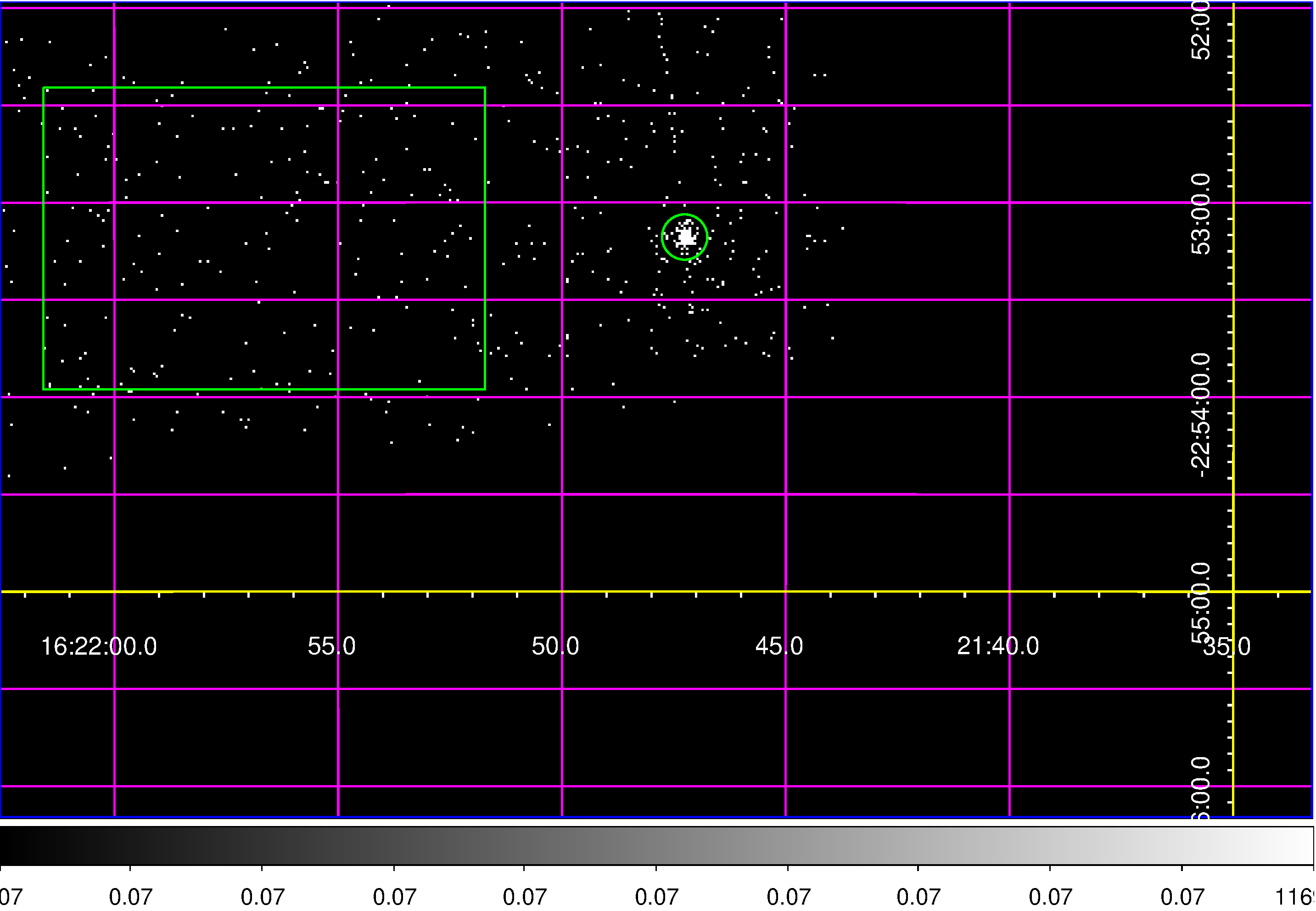
Figure 1: Chandra X-ray image of AR Sco in the energy band of 0.3-7.0 keV showing the source region (circle) and the background region (rectangle) for the extraction of photons used in the analysis.

An X-ray image of AR Sco taken with the SXT is shown in Figure 2. Source counts were extracted from a circular region of 10 arcmin radius centered on AR Sco. Both a light curve and a spectrum were extracted from this region for further analysis.

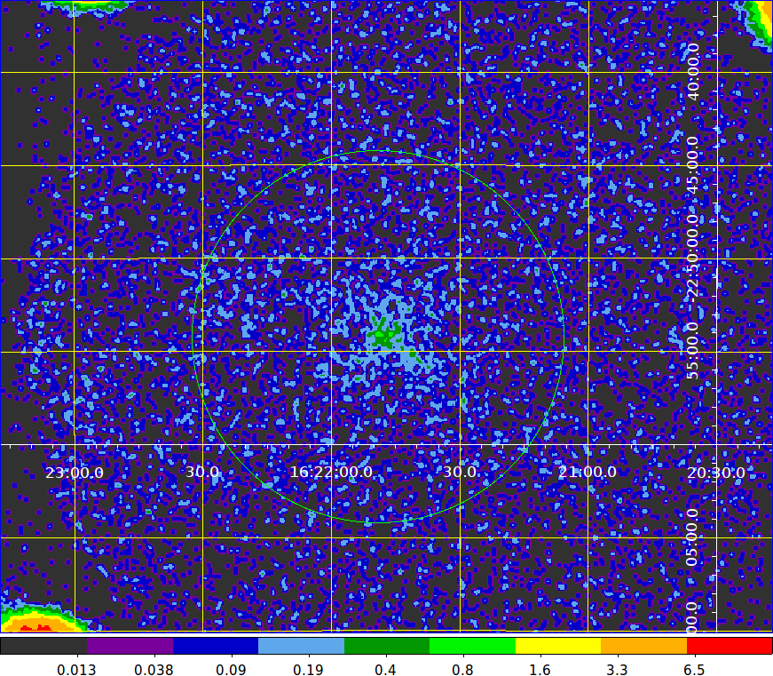
Figure 2: AstroSat SXT image of AR Sco in the energy band of 0.3-7.1 keV showing the circular extraction region of 10 arcmin radius for source counts. Smoothing by a Gaussian with kernel of 3 pixel radius (1 pixel=4 arcsec) has been applied.

3.1 X-ray Light curves

The X-ray light curve in the energy range of 0.3 - 7.0 keV obtained from Chandra observations is shown in Figure 3. The task ’dmextract’ was used to generate the background subtracted source light curve shown. A binsize of 3.364s was used for extraction. The background region was supplied via the ’dmextract’ task parameter ’bkg’.

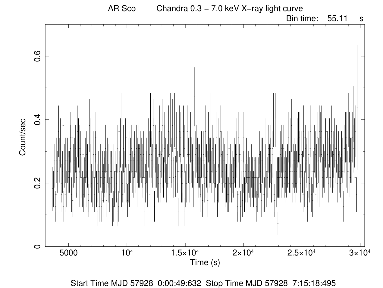
Figure 3: X-ray light curve of AR Sco obtained with the Chandra in the energy range of 0.3-7.0 keV without background subtraction.

The SXT light curve of AR Sco was extracted in the useful energy band of 0.3 $-$ 7.1 keV and is shown in Figure 4. The light curve was extracted with the highest time resolution of 2.3775s. We also extracted the light curves in the soft energy band of 0.3-2.0 keV from both the $Chandra$ and SXT data, where most of the modulation was seen by Takata et al. (2018), and studied their power spectra.

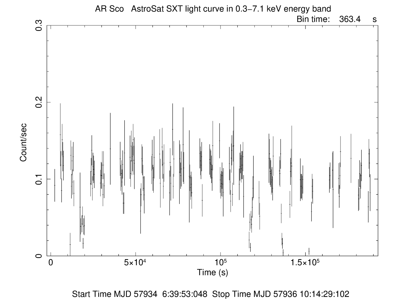
Figure 4: X-ray light curve of AR Sco obtained with the AstroSat SXT in the energy range of 0.3-7.1 keV without any background subtraction.

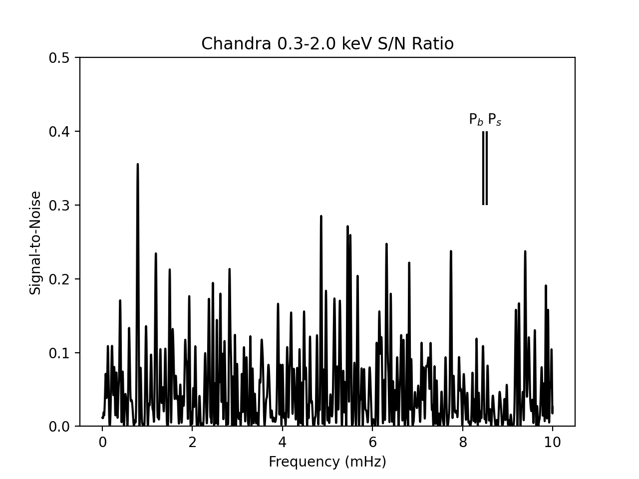
Figure 5: Signal-to-Noise ratio at each frequency in mHz for the $Chandra$ 0.3-2.0 keV data, obtained after applying the DFT. The S/N is $<$1 for all frequencies, so the data show no obvious signal at the spin, orbital, or beat periods. The two vertical lines mark the spin and beat frequencies.

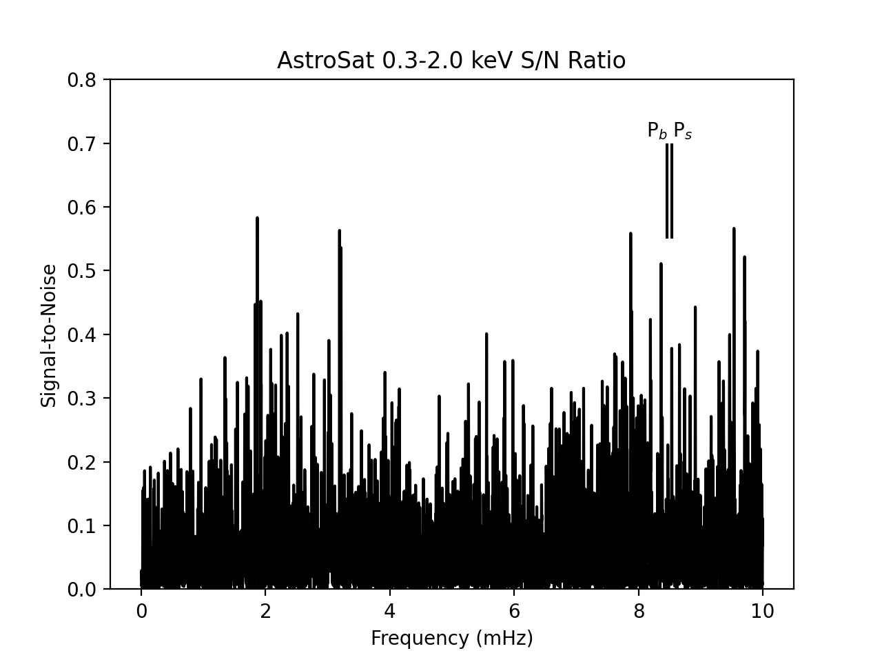
Figure 6: Similar to Fig. 5 for SXT 0.3 - 2.0 keV light curve. The S/N is $<$1.5 for all frequencies showing no obvious signal at the spin, orbital, or beat periods. The two vertical lines mark the spin and beat frequencies.

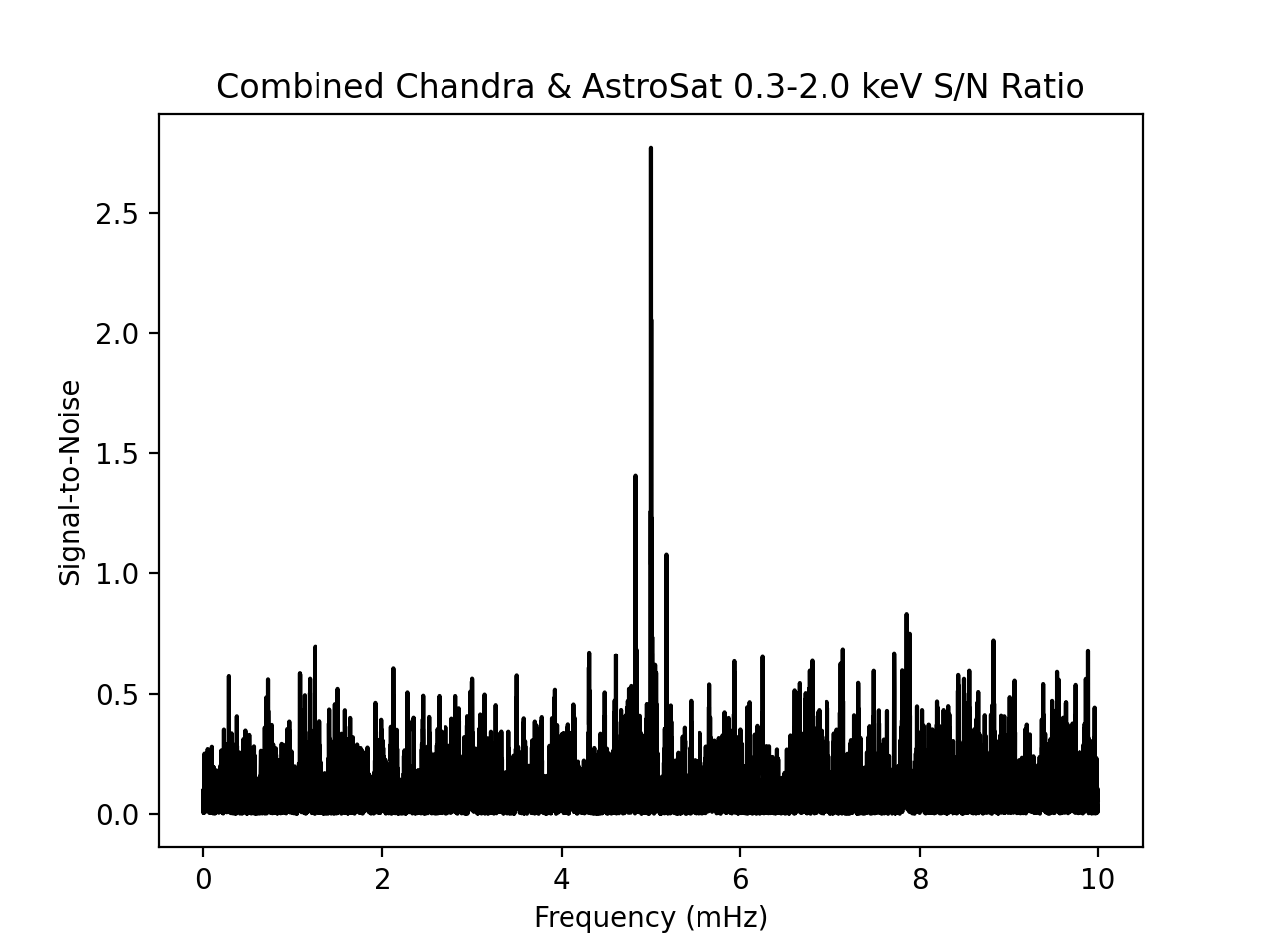
Figure 7: Same as above but with the combined $Chandra$ and AstroSat data injected with a 0.03 counts s^-1 Poisson sinusoid. This simulation implies that any modulation of the spin, orbital, and beat periods is less than about 10% in soft X-rays.

Barycentric corrections are applied to both of the light curves shown in Figs. 3 and 4. The light curves are analyzed using the algorithm of Bretthorst (1988). This algorithm is a formal derivation of the discrete Fourier transform (DFT) using Bayesian statistics and is a generalization of the Lomb-Scargle periodogram (see Appendix A). The signal-to-noise (S/N) ratio of the resulting power spectra for the 0.3–2.0 keV energy band of Chandra and AstroSat are shown in Figures 5 and 6, respectively. Neither figure shows a signal (or peak) having a S/N ratio of $>5$, or equivalently a significance of $>99$%, indicating that no signal is detected. Figure 7 shows S/N obtained for the combined Chandra and AstroSat light curves that include an injected sinusoidal Poisson signal with an amplitude of 0.03 counts s^-1 at a frequency of 5 mHz. The S/N ratio of the dominant signal is about 3 or a likelihood of $>$90%. Note that the S/N ratio decreases quickly from about 3 to 1 between 0.03 to 0.025 counts s^-1. Based on this simulation, any modulation of the spin, orbital, and beat periods in the combined Chandra and AstroSat soft X-ray data are limited to less than about 0.03 counts s^-1, or a modulation amplitude of less than about 10%, assuming an average count rate of 0.3 counts s^-1. Takata et al. (2018) report an $\approx$14% pulse fraction of the beat period in the XMM-Newton $0.15-0.20$ keV X-ray data and essentially no modulation in the $2-12$ keV data from XMM-Newton, thus indicating that the pulse fraction decreases rapidly with increasing energy. We conclude that this spectral characteristic combined with the lower energy cutoff of the XMM-Newton X-ray band compared to that of AstroSat (0.15 keV vs 0.3 keV), and a small change in the X-ray pulse fraction between the 2016 and 2017 observations, is the reason for the non-detection of the beat period by AstroSat and Chandra.

3.2 X-ray Spectra

X-ray spectra were extracted from both the Chandra and SXT observations. The filtered events file from Chandra observation was used for extraction of spectra and responses (Ancillary Response Function (ARF) and spectral Response Matrix File (RMF)) with the CIAO task ’specextract’. The background region was supplied via the task parameter ’bkgfile’. The parameter ’correctpsf=yes’ was used to apply point-source aperture correction to the source ARF file.

For the SXT data, a background spectral file ${SkyBkg\_comb\_EL3p5\_Cl\_Rd16p0\_v01.pha}$, derived from a composite of several deep blank sky observations, distributed by the instrument team is used for spectral analysis for all the spectra analysed here. We used ${sxt\_arf\_excl00\_v04\_20190608.arf}$ as the ARF, and ${sxt\_pc\_mat\_g0to12.rmf}$ as the RMF for the SXT in this work. All these files are available at the SXT POC website $https://www.tifr.res.in/~{}astrosat\_sxt/index.html$.

The source spectra from both the observations were grouped using the grppha tool to ensure a minimum of 25 counts per energy bin, prior to further analysis here and below. The average spectra obtained after background subtraction are shown in Figure 8. We obtained a net count rate of 0.17 $\pm$ 0.0026 s^-1 for the Chandra data and 0.034$\pm$ 0.0012 s^-1 in the SXT spectrum in the energy range 0.7$-$7.0 keV, used for a joint spectral analysis. We confined ourselves to the low energy limit of 0.7 keV instead of 0.3 keV as the background subtraction for this very weak source in the SXT indicated almost negligible flux below 0.7 keV while the flux in the Chandra data at this low energy was slightly higher. This small discrepancy below 0.7 keV, though not statistically significant, would have compromised the value of the column density obtained. A line at 6.7 keV is observed clearly (Figure 8) in the X-ray spectrum obtained from the $Chandra$ observations. The line which is very close to the line expected from ionised Fe XXV indicates thermal emission in the source.

The two spectra were fitted jointly with a simple plasma emission models apec using the xspec program (version 12.9.1; Arnaud (1996) distributed with the heasoft package (version 6.20)). The atomic data base AtomDB version 3.0.7 ($http://www.atomdb.org$), was used. We used a common absorber model Tbabs as a multiplicative model with the model parameter N_H, i.e., the equivalent Galactic neutral hydrogen column density. The plasma temperature (kT) and N_H parameter were kept free, at least initially. We used the abundance table ${}^{\prime}aspl^{\prime}$ given by Asplund et al. (2009) for our analysis, and the abundances of all the elements were tied together and could be varied together with respect to the solar values as one parameter. The normalisation for the plasma component was kept free for the two spectra, and $\chi^{2}$ minimisation technique was used to find the best fit parameters. The column density, N_H, was fixed at the low value of 0.1$\times$10²¹ cm^-2 after it was found to be tending toward zero. This simple model, when fitted to the spectra in the energy range of 0.7 -7.0 keV, gave a good fit with a plasma temperature $\sim$4 keV and solar elemental abundances. The best-fit values for this and other models used for fitting are given in Table 1. The normalisation of the apec model for the two sets of data differ only by $\sim$7%, most probably due to systematic differences in the calibration of the two instruments used. The total flux obtained for the energy band of 0.5-10 keV is found to be (2.5$\pm$0.8$)\times$10^-12 ergs cm² s^-1.

Assuming non-solar abundances for all the elements improved the fit only slightly. We have explored the possibility of an additional thermal component: a black body or a plasma component at different temperature. Addition of either of these gave a significant improvement in the $\chi^{2}$ (and based on the F-statistic values) as can be seen in Table 1, with the maximum improvement coming from the addition of another thermal component. The additional blackbody component was best fit for a temperature of 0.13 keV, but it required a significant absorption column density of 1.8-6.7$\times$10²¹cm^-2 for solar abundances and 2.3-8.2$\times$10²¹cm^-2 (90% confidence range) for non-solar abundances. The best fit to the two-temperature plasma models requires a low temperature component of 0.95${}^{+0.20}_{-0.19}$ keV and a high temperature component of 5.0${}^{+0.8}_{-0.7}$ keV, elemental abundance of 0.6$\pm$0.3 solar, and a negligible N_H in the range of (0.0-2.1)$\times$10²¹cm^-2. We also tried two-component $mekal$ plasma models to compare with the results of Takata et al. (2018), and found very similar results, except for the low-temperature component which gave the best fit for a temperature of 0.77${}^{+0.18}_{-0.16}$, slightly lower but consistent within the errors with that obtained from XMM-Newton data by Takata et al. (2018).

Table 1: Spectral Parameters obtained from a joint fit to the Chandra and SXT spectra (0.7 - 7.0 keV).

Spectral Model				Parameters
	N${}_{H}^{a}$	kTapec	Zb	A1c(C,S)	kTbb/apec	A2c(C,S)	$\chi^{2}_{\nu}$/dof	Flux${}^{d}_{A}$	Flux${}^{d}_{B}$
		keV			keV			(C,S)	(C,S)
tbabs*apec	0.1	4.3${}^{+0.4}_{-0.3}$	1.0	1.55 ,1.66			1.39/274	0.97,1.04	1.43,1.53
tbabs*apec	0.1	4.1${}^{+0.4}_{-0.3}$	0.6${}^{+0.2}_{-0.3}$	1.68 ,1.80			1.30/273	0.97,1.04	1.37,1.47
tbabs*(bbody+apec)	4.7${}^{+2.0}_{-2.9}$	4.1${}^{+1.1}_{-0.6}$	1	1.71,1.70	0.13${}^{+0.03}_{-0.01}$	0.05, 0.06	1.21/270	0.95,1.08	1.49,1.46
tbabs*(bbody+apec)	5.4${}^{+2.8}_{-3.1}$	4.1${}^{+0.8}_{-0.6}$	0.7${}^{+0.3}_{-0.3}$	1.87,1.85	0.13${}^{+0.02}_{-0.01}$	0.07, 0.08	1.20/269	0.93,1.06	1.42,1.39
tbabs*(apec+apec)	0.2${}^{+2.0}_{-0.2}$	5.0${}^{+0.8}_{-0.7}$	1	1.5,1.4	0.94${}^{+0.15}_{-0.18}$	0.06, 0.13	1.20/270	0.97,1.04	1.5,1.4
tbabs*(apec+apec)	0.2${}^{+1.9}_{-0.2}$	5.0${}^{+0.8}_{-0.7}$	0.6${}^{+0.3}_{-0.3}$	1.5,1.4	0.95${}^{+0.20}_{-0.19}$	0.07, 0.15	1.20/269	0.97,1.04	1.5,1.4
tbabs*(mekal+mekal)	0.3${}^{+2.6}_{-0.3}$	4.65${}^{+0.7}_{-0.7}$	0.7${}^{+0.2}_{-0.3}$	1.44,1.37	0.77${}^{+0.18}_{-0.16}$	0.06, 0.14	1.23/269	0.99,1.11	1.44,1.38

^a N_H is in units of 10²¹ cm^-2 ; ^b Abundance, Z, is relative to solar values for all the elements; ^cA1 and A2 are the normalizations for the additive models (as listed) in units of 10^-3 photons cm²s^-1; The letters C and S for A1, A2 and for the flux values refer to $Chandra$ and SXT respectively. ^d Fluxes are in units of 10^-12 ergs cm² s^-1 and are quoted for two energy bands: A for 0.5 - 2.0 keV and B for 2.0 - 10 keV; All errors quoted are with 90% confidence.

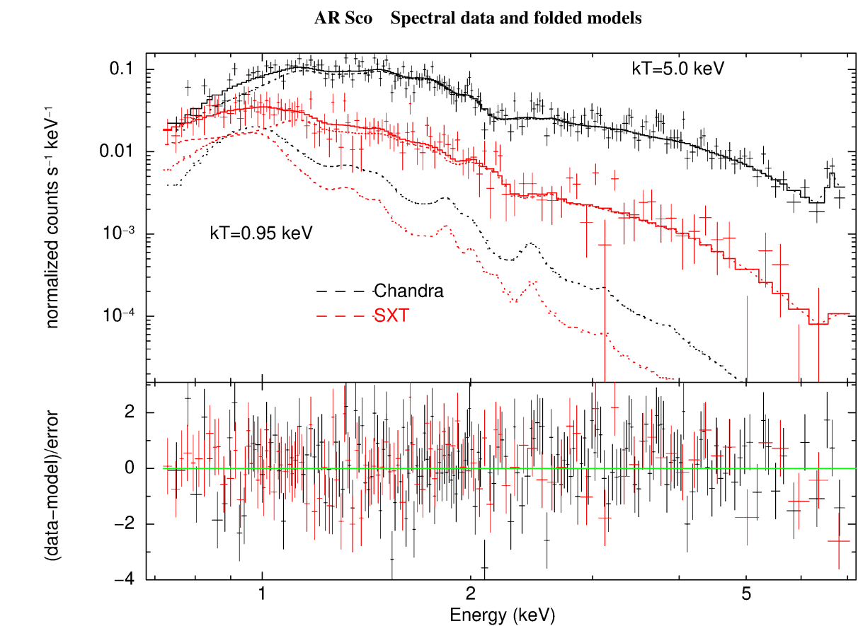
Figure 8: X-ray Spectra of AR Sco (top) along with the best fit 2-temperature plasma models (apec) shown as histograms. Contribution of each component of the plasma model is shown separately as dotted and dash curves, while the solid line histogram shows the combined contribution from the two components. The rms-normalised residuals per channel are shown in the bottom panel.

4 Discussion and Conclusion

Our X-ray observations of AR Sco were carried out in 2017, June-July within a few days of each other with $Chandra$ and AstroSat SXT, and about nine months after the XMM-Newton observations (2016 Sept 19). We find that although on average AR Sco appears about 30% fainter this is not statistically significant given our errors. We find that the spectral data from the two instruments can be fit with the same models with remarkable agreement of normalization to within 7% of each other. The spectra are clearly thermal as significant emission due to the presence of an ionised iron (Fe XXV) line is seen clearly in the $Chandra$ spectrum. The Fe line was also reported earlier by Takata et al. (2018) in the XMM-Newton spectrum. The best-fit spectral models favour two temperature plasma apec models with the best fit high temperature ($\sim$5 keV) component differing from $\sim$8 keV obtained from XMM-Newton observations. It should be noted, however, that the SXT has a negligible effective area above the 7.1 keV limit used here, and Chandra has a very low area above 8.0 keV, and in this particular case the Chandra data above 7.0 keV were flagged as unusable. This could be the reason for the difference in the estimated high energy component. The low-temperature component ($\sim$1 keV) and the low column density (negligible) are in agreement, however.

The time series analysis of the Chandra and AstroSat soft X-ray data show no periodicities at the WD spin period, the orbital period, or the beat period of the two. We believe that the lack of such periodicities is due to the lower sensitivity of the Chandra and AstroSat X-ray telescopes compared to that of XMM-Newton. The XMM light curve contains about 20000 counts, while those of Chandra and AstroSat SXT contain about a factor of ten less or about 2000 counts. Therefore, the relative noise in the Chandra and AstroSat periodograms are about a factor of three larger. We also note that the counting statistics are Poissonian because of the low count rates, which may increase the noise in the data caused by quantization error. It is possible that longer exposures by either of these two telescopes may increase the sensitivity enough to detect a modulation of the soft X-ray flux.

Appendix A

Arthur Schuster (1905) introduced the periodogram near the beginning of the 20th century and this algorithmic technique has been discussed by many authors since that time; including Lomb (1976) and Scargle (1982) for which the Lomb-Scargle algorithm is known by the astronomical community. The periodogram $C(\omega)$ is defined as the squared magnitude of the discrete Fourier transform of the data $D={d_{1},d_{2},...,d_{N}}$:

$$C(\omega)=\frac{1}{N}\Big{[}R(\omega)^{2}+I(\omega)^{2}\Big{]}=\frac{1}{N}\Bigg{|}\sum_{j=1}^{N}d_{j}e^{iwt_{j}}\Bigg{|}^{2},$$ (1)

where

$$R(\omega)=\sum_{i=1}^{N}d_{i}\cos(\omega t_{i})$$ (2)

and

$$I(\omega)=\sum_{i=1}^{N}d_{i}\sin(\omega t_{i}).$$ (3)

A generalization of the periodogram for any time series function was derived using Bayesian principles by Bretthorst in his Ph.D. thesis (1988). The monograph is available for free download at https://bayes.wustl.edu/glb/book.pdf. The following is a brief presentation of Chapters 3 and 4, ’The General Model Equation Plus Noise’ In the most general model, the hypothesis H is

$$H\equiv f(t)=\sum_{j=1}^{m}B_{j}G_{j}(t,\{\omega\}),$$ (4)

where $f(t)$ is some analytic expression of the time series, $G_{j}(t,\{\omega\})$ is a particular model function, $B_{j}$ is the amplitude of the model, and $\{\omega\}$ is a set of parameters (in our case, frequencies). The Bayesian likelihood function for data $D$ is

$$L(\{B\},\{\omega\},\sigma)\propto\sigma^{-N}\exp\Bigg{\{}-\frac{NQ}{2\sigma^{2}}\Bigg{\}}$$ (5)

where

$$Q\equiv\overline{d^{2}}-\frac{2}{N}\sum_{j=1}^{m}\sum_{i=1}^{N}B_{j}d_{i}G_{j}(t_{i})+\frac{1}{N}\sum_{j=1}^{m}\sum_{k=1}^{m}g_{jk}B_{j}B_{k},$$ (6)

$$g_{jk}=\sum_{i=1}^{N}G_{j}(t_{i})G_{k}(t_{i}),$$ (7)

and $\sigma$ is the standard deviation of the noise. $Q$ is an $m\times m$ matrix that can be orthogonalized, resulting in a set of eigenvectors of the likelihood equation. Therefore $f(t)$ can be written in terms of a set of orthonormal functions:

$$f(t)=\sum_{k=1}^{m}A_{k}H_{k}(t),$$ (8)

where

$$A_{k}=\sqrt{\lambda_{k}}\sum_{j=1}^{m}B_{j}e_{kj},$$ (9)

$$B_{k}=\sum_{j=1}^{m}\frac{A_{j}e_{jk}}{\sqrt{\lambda_{j}}},$$ (10)

and

$$H_{j}(t)=\frac{1}{\sqrt{\lambda_{j}}}\sum_{k=1}^{m}e_{jk}G_{k}(t).$$ (11)

A change of functions (6) and variables (8) gives the joint likelihood of the new parameters

$$L(\{A\},\{\omega\},\sigma)\propto\sigma^{-N}\exp\Bigg{\{}-\frac{N}{2\sigma^{2}}\Bigg{[}\overline{d^{2}}-\frac{2}{N}\sum_{j=1}^{m}A_{j}h_{j}+\frac{1}{N}\sum_{j=1}^{m}A_{j}^{2}\Bigg{]}\Bigg{\}},$$ (12)

where

$$h_{j}\equiv\sum_{i=1}^{N}d_{i}H_{j}(t_{i}),(1\leq j\leq m).$$ (13)

$h_{j}$ is the projection of the data onto the orthonormal model function $H_{j}$. Because we have no knowledge of the amplitudes $A_{j}$, they need to be marginalized, or integrated out, by performing j integrations, which gives the likelihood

$$L(\{\omega\},\sigma)\propto\sigma^{-N+m}\exp\Bigg{\{}-\frac{N\overline{d^{2}}-m\overline{h^{2}}}{2\sigma^{2}}\Bigg{\}},$$ (14)

where

$$\overline{d^{2}}\equiv\frac{1}{N}\sum_{i=1}^{N}d_{i}^{2}$$ (15)

and

$$\overline{h^{2}}\equiv\frac{1}{m}\sum_{j=1}^{m}h_{j}^{2}.$$ (16)

If $\sigma$ is unknown, then it’s considered a nuisance parameter and can be eliminated by integrating over all values using the Jeffreys prior $1/\sigma$. This gives an expression for the probability of the form of the ”Student t-distribution”:

$$P(\{\omega\}|D,I)\propto\Bigg{[}1-\frac{m\overline{h^{2}}}{N\overline{d^{2}}}\Bigg{]}^{\frac{m-N}{2}}.$$ (17)

Although $\{A\}$ and $\sigma$ are described as nuisance parameters when deriving the likelihood of the frequency parameters, they are actually of some interest. Bretthorst shows in Chapter 4 that the first posterior moments, i.e., the expected amplitudes, are:

$$\langle A_{j}\rangle=h_{j},$$ (18)

the second posterior moments are:

$$\langle A_{j}A_{k}\rangle=h_{j}j_{k}+\sigma^{2}\delta_{jk},$$ (19)

the noise variance is:

$$\langle\sigma^{2}\rangle=\frac{1}{N-m-2}\Bigg{[}\sum_{i=1}^{N}d_{i}^{2}-\sum_{j=1}^{m}h_{j}^{2}\Bigg{]},$$ (20)

and the signal-to-noise ratio is:

$$\frac{\rm{Signal}}{\rm{Noise}}=\Bigg{\{}\frac{m}{N}\Bigg{[}1+\frac{\overline{h^{2}}}{\sigma^{2}}\Bigg{]}\Bigg{\}}^{\frac{1}{2}}$$ (21)

References

- [1] Arnaud, K.A., 1996, Astronomical Data Analysis Software and Systems V, eds. G. Jacoby and J. Barnes,p17, ASP Conf. Series volume 101.
- [2] Asplund M., Grevesse N., Sauval A.J. & Scott P. 2009, ARAA, 47, 481
- [3] Bretthorst, G. L. 1988, ”Bayesian Spectrum Analysis and Parameter Estimation”, Lecture Notes in Statistics (eds. Berger, Fienberg, Gani, Krickenber, & Singer, Springer-Verlag), Vol. 48.
- [4] Buckley, D.A.H., Meintjes, P.J., Potter, S.B., Marsh, T.R. & Gänsicke, B.T. 2017, Nature Astronomy, 1, 0029
- [5] du Plessis, L, Wadiasingh, Z., Venter, C., Harding, A.K., 2019, ApJ, 887, 44
- [6] Fullerton A. W., Massa D. L., Prinja R. K., Owocki S. P., Cranmer S. R.,1997, A&A, 327, 699
- [7] Gaia Collaboration, Brown, A. G. A., Vallenari, A., Prusti, T., de Bruijne, J. H. J. et al. 2020, A & A (in press); DOI: https://doi.org/10.1051/0004-6361/202039657
- [8] Gaibor, Y., Garnavich, P. M., Littlefield, C., Potter, S. B., Buckley, D. A. H., 2020, MNRAS, 496, 4849
- [9] Garnavich, P., Littlefield, C., Kafka, S., Kennedy, M., Callanan, P., Balsara, D.S. & Lyutikov, M., 2019, ApJ, 872, 67
- [10] Ikhsanov, N. R. 1998, Astron. Astrophys., 338, 521–526.
- [11] Lomb, N. R. 1976, Adv. Space Sci., 39, 447
- [12] Lyutikov, M., Barkov, M., Route, M., Balsara, D., Garnavich, P., Littlefield, C., 2020, (arXiv:2004.11474)
- [13] Marsh, T. R., Gänsicke, B.T., Hümmerich, S., Hambsch, F.-J., Bernhard, K. , Lloyd, C. , Breedt, E., Stanway, E.R., Steeghs, D.T., Parsons, S.G., Toloza, O. , Schreiber, M.R., Jonker, P.G., van Roestel, J., Kupfer, T., Pala, A.F., Dhillon, V.S., Hardy, L.K., Littlefair, S.P., Aungwerojwit, A., Arjyotha, S., Koester, D., Bochinski, J.J., Haswell, C.A., Frank, P. & Wheatley, P.J. 2016, Nature, 537, 374
- [14] Meintjes, P. J. & Venter, L. A. 2005, MNRAS, 360, 573–582.
- [15] Oruru, B. & Meintjes, P. J., 2012, MNRAS, 421, 1557–1586.
- [16] Peterson, E., Littlefield, C. & Garnavich, P. 2019, AJ, 158, 131
- [17] Potter, S.B. & Buckley, D.A.H. 2018a, MNRAS, 478, L78
- [18] Potter, S.B. & Buckley, D.A.H. 2018b, MNRAS, 481, 2384
- [19] Satyvaldiev, V. On seventeen variable stars. Astron. Tsirk. 1971, 633, 7
- [20] Scargle, J. D. 1982, ApJ, 263, 835
- [21] Schuster, A. 1905, Proc. Roy. Soc. London, 77, 136
- [22] Singh, K. K., Meintjes, P. J., Kaplan, Q., Ramamonjisoa, F. A., Sahayanathan, S. 2020, astro-ph.HE, 2006.12950v1.
- [23] Singh, K. P., Tandon, S. N., Agrawal, P. C., et al. 2014, Proc. SPIE, Space Telescopes and Instrumentation 2014: Ultraviolet to Gamma Ray. 9144, 91441S doi:10.1117/12.2062667
- [24] Singh K. P., Stewart, G. C., Chandra, S. et al. 2016, Proc. SPIE, in Space Telescopes and Instrumentation 2016: Ultraviolet to Gamma Ray. 9905, p. 99051E, doi:10.1117/12.2235309
- [25] Singh, K. P., Stewart, G. C., Westergaard, N. J., et al. 2017, JApA, 38, 29
- [26] Starrfield S., Iliadis C., Hix W. R. 2008, in Bode M. F., Evans A., eds, Classical Novae, 2nd edition, Cambridge University Press, Cambridge, p. 77
- [27] Stiller, R. A., Littlefield, C., Garnavich, P., et al. 2018, AJ, 156, 150.
- [28] Takata, J., Hu, C.-P., Lin, L.C.C., Tam, P.H.T., Pal, P.S., Hui, C.Y., Kong, A.K.H.,& Cheng, K.S. 2018, ApJ, 853, 106
- [29] Van Loon J. Th. 2008, in Evans A. et al., eds, R S Ophiuchi (2006) and the Recurrent Nova Phenomenon, ASP Conference Series, Volume 401, p. 90