Automated Mathematical Equation Discovery for Visual Analysis

Abstract

Finding the best mathematical equation to deal with the different challenges found in complex scenarios requires a thorough understanding of the scenario and a trial and error process carried out by experts. In recent years, most state-of-the-art equation discovery methods have been widely applied in modeling and identification systems. However, equation discovery approaches can be very useful in computer vision, particularly in the field of feature extraction. In this paper, we focus on recent AI advances to present a novel framework for automatically discovering equations from scratch with little human intervention to deal with the different challenges encountered in real-world scenarios. In addition, our proposal can reduce human bias by proposing a search space design through generative network instead of hand-designed. As a proof of concept, the equations discovered by our framework are used to distinguish moving objects from the background in video sequences. Experimental results show the potential of the proposed approach and its effectiveness in discovering the best equation in video sequences. The code and data are available at: https://github.com/carolinepacheco/equation_discovery_scene_analysis.

Keywords: automated machine learning, equation discovery, local binary patterns

1 Introduction

In the past few decades, the availability of big data, computing power and the breakthroughs in machine learning algorithms have dramatically increased the impact of artificial intelligence (AI) on our society. AI has been successfully applied to solve many challenging tasks, in areas such as computer vision (Deng et al., 2009; Everingham et al., 2010; Krizhevsky et al., 2012; Shi et al., 2016; Hsu et al., 2018; Shaham et al., 2019; Zhengqi et al., 2019; Radosavovic et al., 2019; Xie et al., 2019), speech recognition (Dahl et al., 2013; Maas et al., 2014; Bukhari et al., 2017; Hadian et al., 2018; Stephenson et al., 2019; Schneider et al., 2019), natural language processing (Sutskever et al., 2014; Bahdanau et al., 2015; Wu et al., 2016; Zheng et al., 2019; Lewis et al., 2020), and others. Despite these impressive advances, significant human expertise is still needed to design promising AI algorithms to solve complex task in the most diverse areas.

Until a few years ago, AI algorithms were able to successfully learn to recognize places, objects, or people but they were not good at creating their own plausible data. Nevertheless, everything started to change with the advances in Deep Generative Networks. They try to simulate the “innovation potential” of the human brain by learning the true data distribution of the training set, in order to generate realistic synthetic data in the form of images, video, audio or text. Variational Autoencoders (VAE) (Kingma and Welling, 2014), Generative Adversarial Networks (GAN) (Goodfellow et al., 2014) and their variants are the most popular types of generative models. The basic idea of the VAE is to maximize the lower bound of the data log-likelihood while GAN aims to achieve a balance between Generator $G$ that generates real-like samples from a random noise input and Discriminator $D$ that tries to differentiate $G^{^{\prime}}s$ generated samples from real training data.

Another important breakthrough in the field of machine learning has been the Automated Machine Learning (AutoML). It is not a new concept, the AutoML techniques have been explored by the scientific community since the 1990s (Ripley, 1993; King et al., 1995; Kohavi and John, 1995; Michie et al., 1995; Guyon and Elisseeff, 2003; Chen et al., 2004; Samanta, 2004; Guyon et al., 2008; Escalante et al., 2009; Bergstra and Bengio, 2012; Feurer et al., 2015; Hoffer et al., 2017). Nevertheless, the AutoML techniques have recently received considerable attention from both scientific and industrial communities. This can be explained by the the exponential growth in computing power and data storage capacity that made it possible to automate machine learning pipelines - from pre-processing, feature extraction, feature selection, model fitting and selection, and hyper-parameter tuning with minimal human intervention  (Drori et al., 2018; Hutter et al., 2019; Feurer and Hutter, 2019). AutoML’s popularity has increased further still since 2016 when Google Brain team revealed their first Neural Architecture Search (NAS) (Zoph and Le, 2017). It a subfield of AutoML that allows to automate the manual process to discover the optimal network architecture, which significantly reduces human labor. Given a human-designed search space containing a set of possible neural networks architectures, NAS uses an optimization method to automatically find the best combinations within the search space (Kobler, 2009; Zoph and Le, 2017; Liu et al., 2018; Hutter et al., 2019). Despite the effectiveness of NAS, it still remains laborious to define a useful search space, because it often requires human expert knowledge and involves a process of trial-and-error. In addition, the search space usually relies on human bias, as its design depends on human-designed architectures as starting points.

Currently, research in the field of NAS focuses mainly on discovery of high-performance neural network architectures that were predefined by humans. However, reducing the search space of the human bias can help increase of the innovation potential of NAS, meaning a great breakthrough in the development of AI systems that can create novelties with high performance on their own without human intervention (Hutter et al., 2019; Real et al., 2020). An impressive research recently presented by (Real et al., 2020), showed that AutoML can discover completely new algorithms through a generic search space. They proposed a framework for discovering machine learning algorithms using regularized evolution search method. Inspired by their research, in this paper we propose a novel framework for discovering mathematical equations that even human developers may not have thought of yet with minimal human intervention. Given a search space designed by VAE instead hand-designed containing a set of possible Local Binary Patterns (LBP) equation structures, the Multi-Objective Covariance Matrix Adaptation Evolution Strategy (MO-CMA-ES) (Igel et al., 2007; Hansen, 2011) searches the best LBP equation by mutating its arithmetic operators. Next, the performance of each LBP equation is estimated in a background subtraction problem  (Sobral and Vacavant, 2014) to distinguish the moving objects from a set of videos. Finally, the LBP equation which presented the maximum precision is selected as a best equation for dealing with specific challenges (e.g., changes in lighting, dynamic backgrounds, noise, shadows and others) in a real-world scene.

In summary, our contributions are as follows:

• a search space designed by VAE containing a wide variety of mathematical equation structures that we may never have thought of yet;

• a new framework capable of discovering the most suitable LBP mathematical equations to deal real-world scenarios;

• an extensive experiments to prove the potential of our approach to distinguish moving objects from the background in video sequences.

The remainder of the paper is organized as follows. Section II provides quite a comprehensive overview of state-of-the-art of the equation discovery approaches. Section III introduces our framework by illustrating it on a background subtraction problem. Section IV shows the experimental results which are reported and discussed. Finally, Section V concludes the paper with a summary and a brief outline of some directions for further research.

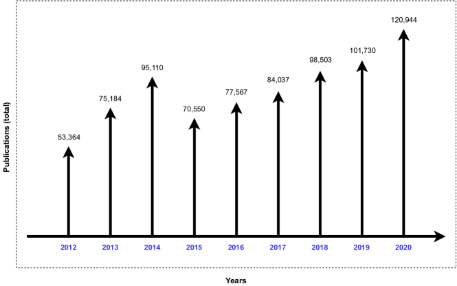
Figure 1: Scientific publications based on LBP from 2012, the year the Convolutional Neural Networks (CNN) achieved a top-5 error of 15.3 in the ImageNet 2012 Challenge, up to 2020. In total, 776.989 LBP research papers were proposed in this period 2012-19 showing the growing interest of the scientific community in the subject. Source: Dimensions (2021).

2 Related Work

Equation discovery is a topic in the machine learning area that automates the process of formulating mathematical equations to find the equation that best fits through data  (Langley, 1995; Mitchell, 1997; Todorovski and Džeroski, 2001). It has achieved remarkable success late 1980s, since publication of the BACON system proposed by Langley et al. (1987a, b). Six versions of BACON have been proposed to rediscover various physical laws, such as the gravitation’s law, the Boyle’s law, the Ohm’s law and others - from experimental data. All BACON system versions share a common approach, as well as a common representation of data and laws for equation discovery. The differences between them are in the set of data-driven heuristics that is used to search for empirical laws. One of the main limitations of the BACON systems is that they do not support irrelevant variables in the input data. Another pioneering system in discovery equations that deals with this restriction is the ABACUS (Falkenhainer and Michalski, 1985). In contrast to BACON, ABACUS allows irrelevant variables to be present in the input data, making the combination of existing variables to formulate new intrinsically exponential variables. To overcome this limitation, ABACUS prohibits mathematically redundant expressions and physically impossible relationships. Other related methods that extend or use approaches similar to BACON and ABACUS are FAHRENHEIT (Zytkow, 1987), IDS  (Nordhausen and Langlay, 1990)  (Shrager and Langley, 1990) and KEPLER  (Wu and Wang, 1989), Coper  (Kokar, 1986a, b) and Fortyniner (Zytkow and Baker, 1991).

Džeroski and Todorovski (1995) proposed LAGRANGE, the first equation discovery approach to dealing with differential equations. It exhaustively searches for the space of polynomial equations with limited number of terms that are based on observed system variables and their time derivatives. LAGRANGE allows the user to define the space of candidate equations by selecting the parameter values, such as the maximum number of terms or maximum degree of the polynomial. Two years later, Todorovski and Džeroski (1997) introduced the successor to the LAGRANGE framework, the LAGRAMGE. Instead of using the model structure provided by a human expert, like most other methods, LAGRAMGE relies on context free grammars to specify a wide range of possible equation structures that make sense from the expert’s point of view. It allows expressing different types of knowledge by grammar, however, it is not very easy for a domain expert to encode their domain knowledge in the form of grammar. Besides, the grammar-based formulation is generally task specific, so a grammar created to model a certain system cannot necessarily be used to model other systems in the same domain. Some years later, Todorovski and Džeroski (2007) extend the LAGRAMGE method by proposing the LAGRAMGE 2.0 version. It provides a formalism for integrating knowledge of population dynamics modeling for discovering equations. This formalism allows the codification of a high level domain knowledge accessible to human specialists. Coded knowledge can be automatically transformed into operational form of context-dependent grammars. The experimental results show that the integration of specialized knowledge within the equation discovery process significantly improves the robustness and efficiency of the LAGRAMGE 2.0 method when compared to the previous version. LAGRAMGE framework has been successfully applied in different real-world applications. For instance,  Ganzert et al. (2010) adapt the LAGRAMGE method to discover mathematical equations that model a mechanically ventilated lung. In (Alzaidi and Kazakov, 2011), the method is used to find equations that predict London Metal Exchange commodity prices.  Markič and Stankovski (2013) also use this method to discover equations in the field of earthquake engineering to predict peak ground acceleration.

Simidjievski et al. (2020) recently presented a process-based approach to discover equations for modeling nonlinear dynamic systems from measurements and domain-specific modeling knowledge. Although the approach has been applied to a cascaded water tank system with two tanks, the authors claim that the proposed method can be applied in a variety of other system identification tasks. Tanevski et al. (2020) shows a knowledge-driven strategy for selecting a suitable structure from a finite set of user-specified equation structures using various combinatorial search algorithms. After carrying out different experiments in reconstructing the structure of dynamical systems models, the authors noticed that using the combination of beam (Bisiani, 1992) and tabu (Glover and Laguna, 1997) search algorithms or particle swarm optimization (Parsopoulos, 2010), achieves the best trade-off between speed of convergence and recall. Nonetheless, search algorithms with moderate diversification are the most suited algorithms to biased equation discovery. Finally, the authors conclude that genetic algorithms showed a lower performance for knowledge-based equation discovery.

Most state-of-the-art equation discovery methods have been widely applied in the modeling and identification systems. However, we believe that equation discovery approaches can be very useful in the scope of computer vision, particularly in the field of feature extraction. Despite the great success of deep learning techniques  (Krizhevsky et al., 2012; Lecun et al., 2015; Goodfellow et al., 2016), a variety of texture extraction methods have recently attracted great attention for different applications, especially the Local Binary Pattern (LBP) (Ojala et al., 2002) because it is simple and quick to calculate. Figure 1 shows a graph of the LBP-based papers proposed since 2012, the year the Convolutions Neural Network (CNN) achieved a top-5 error of 15.3 % in the ImageNet 2012 Challenge, up to 2020. In total 776.989 LBP papers were proposed in the period 2012-19 showing the growing interest of the scientific community for the subject. LBP is a texture descriptor which labels the pixels of an image by establishing a threshold in the neighborhood of each pixel and considers the result as a binary number. It shows great invariance to changes in monotonic lighting, does not require many parameters to be set, and has a high discriminative power. However, sometimes the original LBP equation needs to be reformulated to make it capable to deal with several challenges (e.g., sudden changes in lighting, dynamic backgrounds, camera jitter, noise, shadows, and others) found in different types of scenes. Nevertheless, to formulate a mathematical LBP equation that is robust to the different challenges faced in a complex scene, in-depth knowledge of the scene and trial-error process by experts is required. Therefore, in this paper we focus on recent AI advances to propose a framework to automatically discovering LBP equations from scratch with little human intervention to deal with different challenges encountered in complex scenes.

3 Proposed Method

The proposed approach to discovering equations consists of two main components: (1) Discover the best VAE to design our search space that contains a wide variety of mathematical LBP equation structure that we may never have thought of yet. (2) Search the best LBP equation to deal with different challenges (e.g., changes in lighting, dynamic backgrounds, camera jitter, noise, shadows, and others) faced by a background subtraction algorithm in detecting moving objects found in complex scenarios. We describe each of these components in the remainder of this section.

3.1 Search Space Design by VAE to Generate Equation Structures

The search space design is a key component for equation discovery. In the search space, we must define which equation structures will be designed and optimized. Instead of hand-designed search space, we design it through a Variational Autoencoder (VAE). Given a set of parameters denoted by $S$, the MO-CMA-ES (see subsection 3.2.1 for further details) is responsible for generating a set of parameters to train different VAE’s expressed by $\Psi=\{\psi_{1},\psi_{2},\ldots,\psi_{L}\}$, where $\psi$ represents a VAE instance and $L$ is the maximum number of elements $\psi\subseteq\Psi$. Next, the VAE with the optimum parameters that allow best well-performing is selected. Finally, the $\psi\subseteq\Psi$ which presented the maximum accuracy $\{\arg\max_{j\in 1,\ldots,L}P_{j}(x)\}$ is chosen to design our search space defined as $E$ that will contain a set of new LBP equations. The $P$ defines a set of accuracy for each $\psi\subseteq\Psi$. A brief overview of this first step of our proposed framework is illustrated in Figure 2. The VAE is introduced below.

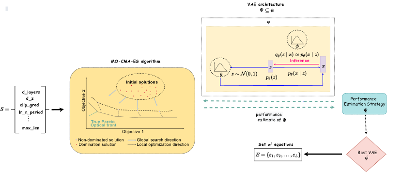
Figure 2: Brief overview of the first component of the proposed framework. Given a set of parameters denoted by $S$, the MO-CMA-ES is responsible for generating a set of optimal parameters to train different VAE’s expressed by $\Psi=\{\psi_{1},\psi_{2},\ldots,\psi_{L}\}$, where $\psi$ represents a VAE and $L$ is the maximum number of elements $\psi\subseteq\Psi$. Then, the VAE with the optimum parameters that allow best performance is selected. Finally, the $\psi\subseteq\Psi$ which presented the highest performance is chosen to design the search space $E$.

3.1.1 Variational Autoencoder (VAE)

Variational Autoencoder (VAE) is a neural network-based generation model that learns an encoder and a decoder that leads to data reconstruction and the ability to generate new samples that share similar statistics from the input data. Given a small set of equations $x$ the VAE maps the $x$ onto a latent space with a probabilistic encoder $q_{\phi}(z\mid x)$ and reconstructs samples with a probabilistic decoder $p_{\theta}(x\mid z)$. A Gaussian encoder was used with the following reparameterization trick:

$$q_{\phi}(z\mid x)=\mathcal{N}(z\mid\mu_{{}_{\phi}}(x),\sigma_{{}_{\phi}}(x))=\mathcal{N}(\in\mid 0,I)\cdot\sigma_{{}_{\phi}}(x)+\mu_{{}_{\phi}}(x)$$ (1)

Gaussian distribution $\mathcal{N}(0,I)$ is the most popular choice for a prior distribution $p{{}_{\psi}}(z)$ in the latent space. The Kullback-Leibler divergence, or simply, the $\mathcal{KL}$ divergence is a similarity measure commonly used to calculate difference between two probability distributions. To ensure that $q(z\mid x)$ is similar to $p(x\mid z)$, we need to minimize the $\mathcal{KL}$ divergence between the two probability distributions.

$$\min\mathcal{KL}(q_{{}_{\phi}}(z\mid x)\|p_{\theta}(z\mid x))$$ (2)

We can minimize the above expression by maximizing the following:

$$L(\phi,\theta:x)=E_{z\sim q_{{}_{\phi}}(z\mid x)}(\log(p_{\theta}(x\mid z))-\mathcal{KL}(q_{{}_{\phi}}(z\mid x)\|p(z))$$ (3)

As we see in Eq.(3), the loss function for VAE consists of two terms, the reconstruction term that penalizes error between the reconstruction of input back from the latent vector and the divergence term that encourages the learned distribution $q_{{}_{\phi}}(z\mid x)$ to be similar to the true prior distribution $p(z)$, which we assume following a unit Gaussian distribution, for each dimension $j$ of the latent space.

Figure 3: Brief overview of the second component of the proposed framework. A set of LBP equations $E=\{\varepsilon_{1},\varepsilon_{2},\dots,\varepsilon_{K}\}$, where $\varepsilon$ expresses each equation structures and $k$ is a user parameter that determines the number of elements $\varepsilon\subseteq E$. Initially, the MO-CMA-ES seeks the best LBP equation by mutating the arithmetic operators of each equation $\varepsilon\subseteq E$ resulting in a new one of the mutated equations $E^{{}^{\prime}}=\{\varepsilon^{{}^{\prime}}_{1},\varepsilon^{{}^{\prime}}_{2},\dots,\varepsilon^{{}^{\prime}}_{K}\}$. The performance of each LBP equation is estimated by a background subtraction algorithm to distinguish the moving objects from the background of a set of videos. Finally, the $\varepsilon^{{}^{\prime}}$ that presented the maximum accuracy is selected as a best equation structure.

Algorithm 1 Equation Structure Discovery

1:  Require: $S=\{{\text{ENC\_LAYERS, DEC\_LAYERS, ENC\_HIDDEN, DEC\_HIDDEN, etc.}}\}$, training set images $X$, user parameter $L$, VAE instance $\nu$, MO-CMA-ES instance, arithmetic operators $A=\{+,-,*,/\}$, user parameter $K$

2:  l $\leftarrow 1$

3:  repeat

4:  for $l=1:L$ do

5:     // search the best VAE $\psi$

6:     $\psi_{l}\leftarrow$ MO-CMA-ES ($\nu$ ,$S$)

7:     $P_{l}\leftarrow$ Performance-Estimation($\psi_{l})$

8:     vae-scores $\leftarrow$ {$P_{l}$, $\psi^{{}^{\prime}}_{l}\}$

9:  end for

10:  // Select the best VAE

11:  {$P$, $\psi\}$ = $\arg\max(\textit{vae-scores})$

12:  

13:  // generate a set of LBP equation structure $E=\{\varepsilon_{1},\varepsilon_{2},\dots,\varepsilon_{K}\}$ using the best VAE $\psi$

14:  k $\leftarrow 1$

15:  repeat

16:  for $k=1:K$ do

17:     // generate a set of LBP equations $\varepsilon^{{}^{\prime}}$ by mutating their arithmetic operators $A=\{+,-,*,/\}$

18:     $\{\varepsilon^{{}^{\prime}}_{t}\}\leftarrow$ MO-CMA-ES ($\varepsilon$, A)

19:     $P^{{}^{\prime}}_{k}\leftarrow$ Background-Subtraction-Method($\varepsilon^{{}^{\prime}}_{k},X)$

20:     lbp-scores$\leftarrow$ {$P^{{}^{\prime}}_{k}$, $\varepsilon^{{}^{\prime}}_{k}\}$

21:  end for

22:  // Select the best equation

23:  {$P^{{}^{\prime}}$, $\varepsilon^{{}^{\prime}}\}$ = $\arg\max(\textit{lbp-scores})$

24:  Output: Best $\varepsilon^{{}^{\prime}}$ equation and its accuracy

3.2 Search Strategy by MO-CMA-ES to Discover the Best Equation

With a search space designed, $E=\{\varepsilon_{1},\varepsilon_{2},\dots,\varepsilon_{K}\}$, where $\varepsilon$ expresses each equation structures and $K$ is a user parameter that determines the number of elements $\varepsilon\subseteq E$, the MO-CMA-ES looks for the best LBP equation by mutating the arithmetic operators $(+,-,*,/)$ of each equation $\varepsilon\subseteq E$ resulting in a new set of mutated equations given by $E^{{}^{\prime}}=\{\varepsilon^{{}^{\prime}}_{1},\varepsilon^{{}^{\prime}}_{2},\dots,\varepsilon^{{}^{\prime}}_{K}\}$. We estimate the performance of each LBP equation by using a background subtraction algorithm called Texture BGS (Heikkila and Pietikainen, 2006). Alows us to distinguish moving objects from the background of a set of videos. Finally, the $\varepsilon^{{}^{\prime}}\subseteq E^{{}^{\prime}}$ that presented the maximum accuracy $\{\arg\max_{j\in 1,\ldots,K}P^{{}^{\prime}}_{j}(x)\}$ is chosen to deal with a particular challenge that is commonly encountered in complex scenes (e.g., changes in lighting, dynamic backgrounds, camera jitter, noise, shadows and others). The $P^{{}^{\prime}}$ represents a set of accuracy for each $\varepsilon^{{}^{\prime}}\subseteq E^{{}^{\prime}}$. A complete description of all steps of the proposed framework is presented in Algorithm 1. The Figure 3 shows a brief illustration of this step of our framework. An introduction of the MO-CMA-ES is described below. A state-of-the-art with a detailed description of the MO-CMA-ES can be found in (Igel et al., 2007; Hansen, 2011).

3.2.1 Multi-Objective Covariance Matrix Adaptation Evolution Strategy (MO-CMA-ES)

Multi-Objective Covariance Matrix Adaptation Evolution Strategy (MO-CMA-ES) is a search strategy algorithm that ranks the elements in a population $A$ of candidate solutions according to their level of non-dominance. It is based on two hierarchical criteria: Pareto ranking and hypervolume contribution. Let the non-dominated solution in $A$ be represented by ndom(A) = $\{a\in\mathrm{A}\mid\nexists a^{{}^{\prime}}\in\mathrm{A}:a^{{}^{\prime}}\prec a\}$, where $\prec$ indicates the Pareto-dominance relation. The Pareto front of $A$ is then given by $\{{(f_{1}(x),\ldots,f_{m}(a))\mid a\in{\text{ndom(A)}}}\}$, where the $f_{i}$ are the $m$ real-valued objective functions. Initially, the Pareto by interactively process ranks the elements in ndom(A) a level of non-dominance getting rank 1. The other ranks of non-dominance continue until all points of $A$ have received a Pareto rank. Next, the solutions that have the same level of non-dominance are ranked by considering the contributing hypervolume. The hypervolume measure or $\mathcal{S}$-metric (Zitzler and Thiele, 1998) is determined in as follows:

$$\mathcal{S}_{f^{ref}}(A)=\land\left(\bigcup_{a\in A}\left[f_{1}(a),f_{1}^{ref}\right]\times\cdot\cdot\cdot\times\left[f_{m}(a),f_{m}^{ref}\right]\right)$$ (4)

where $f^{ref}\in\mathbb{R}^{m}$ indicates an appropriately selected reference point and $\land(\cdot)$ (i.e., the volume) being Lebesgue measure. The contributing hypervolume of a point $a\in A^{{}^{\prime}}$= ndom(A) is given according by $\bigtriangleup_{\mathcal{S}}(a,A{{}^{{}^{\prime}}})=\mathcal{S}_{f^{ref}}(A^{{}^{\prime}})-\mathcal{S}_{f^{ref}}(A^{{}^{\prime}}\backslash\{a\})$. Element $a$ with the lowest contributing hypervolume is assigned to contribution rank 1.

Finally, in the MO-CMA-ES version considered in this paper, an individual offspring $a^{{}^{\prime}(g+1)}_{i}$ is determined to be successful if selected for the next parent population $P^{(g+1)}=\{Q^{g}_{\prec:i}\mid 1\leq i\leq\mu\}$:

$$succ_{Q^{(g)}}^{P}\left(a_{i}^{(g)},a^{{}^{\prime}(g+1)}_{i}\right)=\begin{cases}1&\text{if $a_{i}^{{}^{\prime}(g+1)}\in Q^{(g+1)}$}\\ 0&\text{otherwise}\end{cases}$$ (5)

where succ${}_{Q^{(g)}}^{P}\left(a_{i}^{(g)},a^{{}^{\prime}(g+1)}_{i}\right)$ in Eq.(5) is success indicator. It evaluates as one if the mutation that created $a^{{}^{\prime}(g+1)}_{i}$ is considered successful and zero otherwise.

4 Experimental Results

In this section, we evaluate each component of our proposed method by conducting different experiments. First, we start by finding the set of optimal hyperparameters to train a VAE instance that generates a set of valid equations that are different from those within the training set. Therefore, we defined an evaluation measure called number of Unseen & Valid Equations (UVE), and our main objective in this first experiment was to find a configuration for the VAE instance that maximizes the UVE measure. Each VAE instance with specific hyperparameters generates a set of equations, so its validity is verified by a regular expression. As a search strategy algorithm, we choose the MO-CMA-ES due to its simplicity and scalability to higher dimensional problems. In addition, it is parallelizable and easily distributed. This can be a very important factor in AutoML approaches that spend a lot of computational time. To perform the experiments optimally, we use the Proactive Machine Learning (PML) . It is an open source solution developed by Activeeon that allows researchers to easily automate and orchestrate AI-based workflows, scaling-up with parallel and distributed execution in any type of infrastructure: on premise, hybrid, multi-cloud or HPC (High Performance Computing), by taking into account full computing capacity, from CPU to GPU/TPU/FPGA. PML allows hyperparameter optimization on a large scale, and users are free to implement their own machine learning algorithms using different programming languages such as Python, MATLAB, R, C, Java etc.

We implemented the proposed framework using PyTorch 1.0 and Python 3.6. The experiments were conducted on an NVIDIA GeForce RTX 2070 graphics card with 3.5 GHz Intel i7-3770K CPU that consists of 4 cores and 8 threads, and 16GB of RAM. First, we ran 150 interactions of two parallel instances of the VAE with different hyperparameters using the PML platform. VAE models are based on the Gated Recurrent Unit (GRU) (Cho et al., 2014). It’s an enhanced version of the standard recurrent neural network that aims to solve the vanishing gradient problem. The GRU can also be known as a variation on the Long short-term memory (LSTM) (Hochreiter and Schmidhuber, 1997) because both are similarly designed and, in some cases, produce equal results. Nevertheless, we choose to use GRU instead of LSTM because it has less training parameters and therefore uses less memory, running time and trains faster. We trained our model into 150 epochs using an early stopping mechanism. Therefore, we seek to minimize the KL-divergence and the reconstruction loss. In Table 1, we tabulate the hyperparameters used in the VAE network and in the training stage. The first column contains the definitions of each parameter. In the second column the range value that each of these parameters can assume and finally the last column shows the combination of the best values for each parameter. The set of the best parameter values were used the configuration of our VAE that will be responsible for generating our search space containing a set of equations. Note that the choice represents a list of possible values or parameters for each variable.

Hyperparameter	Range Values	Best Values
VAE network parameters
ENC_HIDDEN - Number of features in the hidden of the encoder	choice([125, 256, 512])	125
DEC_HIDDEN - Number of features in the hidden of the decoder	choice([512, 800])	512
ENC_LAYERS - Number of recurrent layers of the encoder	choice([1, 2, 4, 6])	6
DEC_LAYERS - Number of recurrent layers of the decoder	choice([1, 2, 4, 6])	1
ENC_DROPOUT - Dropout rate of the encoder	choice([0.01, 0.02, 0.01, 0.1, 0.2])	0.1
DEC_DROPOUT - Dropout rate of the decoder	choice([0.01, 0.02, 0.01, 0.1, 0.2])	0.01
Training parameters
N_BATCH - Samples per batch to load	choice([32, 64, 512])	32
LEARNING_RATE - Learning rate	choice([0.001, 0.005])	0.005
OPTIMIZER - Optimization algorithms	choice([Adam, Adadelta, RMSprop])	RMSprop

• ^⋆ If (ENC_LAYERS) or (DEC_LAYERS) $>$ 1, becomes a bidirectional GRU otherwise unidirectional GRU.

Table 1: List of hyperparameters used in the VAE network and in the training stage. In the second column the range value that each of these parameters can assume and finally the last column shows the combination of the best values for each parameter. The set of the best parameter values is used as the configuration of our VAE that will be responsible for generating our search space containing a set of equations.

In Figure 4, we can see an overview of how the different instances of VAE behave when varying the values of their hyperparameters to maximize the UVE measure. Some hyperparameters values are important, while others could even be eliminated, thereby reducing our initial set of hyperparameters. For instance, the ENC_HIDDEN: 125, 256, DEC_HIDDEN: 512, ENC_LAYER: 4, 6, DEC_LAYER: 1, ENC_DROPOUT: 0.01, 0.1, 0.2, DEC_DROPOUT: 0.01, OPTIMIZER: RMSpop, N_BATCH: 32 and LEARNING_RATE: 0.05 were parameter values that contributed to maximize the number of UVE. Figure 5 shows the importance of each hyperparameter when trying to maximize the UVE measure. As we can see the ENC_DROPOUT, ENC_LAYERS and DEC_DROPOUT were the hyperparameters that most impacted on VAE training. This can be explained by the fact that the dropout layer is very important in Generative Network architectures because they pre-

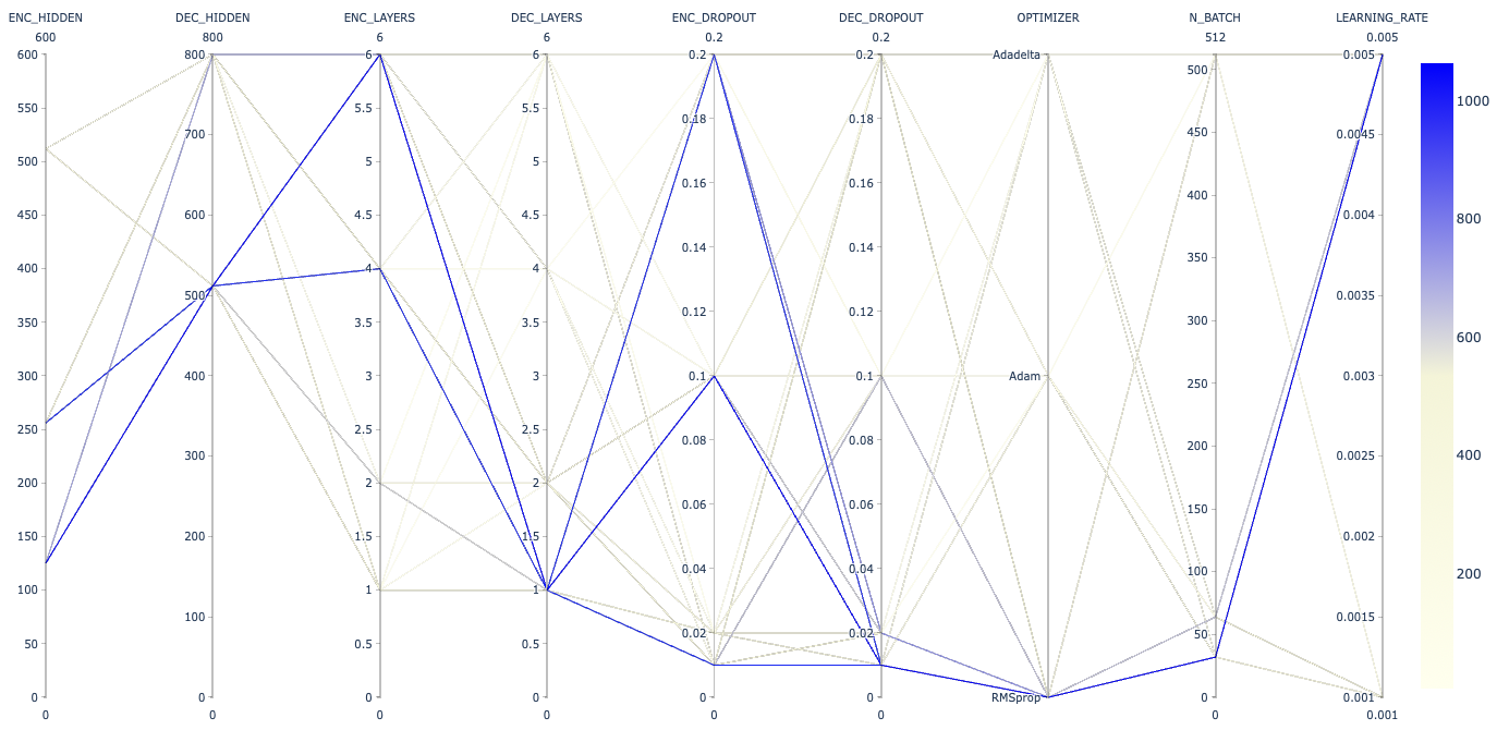
Figure 4: Different hyperparameters used in the VAE. An overview of how the different instances of VAE behave when varying the values of their hyperparameters to maximize the UVE measure.

vent all neurons in a layer from synchronously optimizing their weights preventing all the neurons from converging to the same goal, thus decorrelating the weights. Another hyperparameter that normally positively impacts the performance of the generative neural models is the number of recurrent layers in the encoder. A study presented by Wu et al. (2016) showed that the 2-layer bidirectional encoder performed slightly better than other tested configurations. However, in Figure 4 we can see that 4 or 6 bidirectional layers provided better results to solve our problem, thus reinforcing the theory that deeper networks achieve better performance than shallow networks. A curious fact is that the number of decoder layers did not have a major positive impact on the performance of the VAE models in this work. This behavior could be explained by the fact that the encoder layers as well as its dropouts played a more important role during the equations generation than the decoder layers. Once we define a set of optimal hyperparameters for VAE model, it generated a set of 305 valid and unique LBP equations structures. They are based on the LBP modified by Heikkila and Pietikainen (2006) for background modeling. The authors proposed to modify the threshold scheme of the original LBP equation, replacing the term $s(Z-C)$ with the $s(Z-C+a)$ where $C$ corresponds to the gray value of the center pixel of a local neighborhood, $X$ to the gray values of $P$ pixels equally spaced on a circle of radius R and $a$ is a small value. Note that in our experiments $a$ is defined as 0.01. The modified LBP improves the original LBP equation in image areas where the gray values of the neighboring pixels are very close to the center pixel, e.g. sky, grass, etc. The MO-CMA-ES changed each LBP equation using $4^{n}$ permutations, where $4$ is the number of the types of arithmetic operations $[+,-,*,/]$) and $n$ is number of arithmetic operators presented in the equation. However, to prevent the generation of exponential mutations, we limited our experiment to $4^{5}=1024$ mutations. In order to verify if the mutated equations are useful for dealing with different challenges found in real-world scenarios, we consider as our performance estimation strategy a background subtraction algorithm called Texture BGS proposed by Heikkila and Pietikainen (2006) and a set of real-world scene sequences from CDnet-2014 data set (Wang et al., 2014). A brief description of the Texture BGS algorithm and CDnet-2014 are presented below:

• Texture BGS method: it is a non-parametric approach that models each pixel as a group of adaptive LBP histograms that are calculated over a circular region around the pixel. Initially, the LBP histogram of the given pixel is calculated from the new video frame and compared to the current model histograms using an intersection measure of the histogram. Then, the histogram’s persistence in the model is used to decide whether the histogram models the background or not. The higher the weight, the more likely it is a background histogram. At the end of the updating procedure, the model’s histograms are ordered in descending order according to their weights, and the first histograms are select as background histograms.

• CDnet-2014 data set: it is the largest data set with videos that contains several motion and change detection challenges, in addition to typical indoor and outdoor scenes that are found in most surveillance, smart environments, and video analytics applications. The CDnet data set contains 53 annotated videos from various real-world scenarios. These videos are categorized into 11 categories such as bad weather, low framerate, night videos, PTZ, thermal, shadow, intermittent object motion, camera jitter, dynamic background, baseline and turbulence.

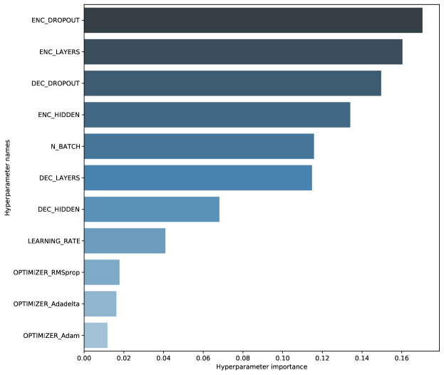
Figure 5: Hyperparameters Importance. The ENC_DROPOUT, ENC_LAYERS and DEC_DROPOUT were the hyperparameters that had the greatest impact on training.

Each mutated LBP equation was evaluated using the Texture BGS method in ’peopleInShade’, ’snowFall’, ’canoe’, ’busStation’, ’skating’, and ’fall’ sequences with resolutions 180 x 120 pixels. The description of each scene and its main challenges are presented in Table 2. We limited the number of sequence for each scene around 7 $\sim$ 40 frames due to the limitation of computational resources, since our approach has high computational complexity and computation time. All equations were performed in parallel thanks to the PML platform. We present the visual results on individual frames from six different scenes: ’peopleInShade’ (frame #318), ’snowFall’ (frame #2758), ’canoe’ (frame #904), ’busStation’ (frame #300), ’skating’ (frame #1845) and ’fall’ (frame#3987) of the CDnet-2014 data set. Figures 6 and 7 show the foreground detection results using the Texture BGS and the proposed method, respectively. They were shown without any post-processing technique. The results obtained by using the best LBP equations discovered by the proposed method (see Table 2) clearly appears to be less sensitive to background subtraction challenges and are able to detect moving objects with fewer false detection, especially in the ’canoe’ video which is a complex scene with a strong background motion and in the ’skating’ scenes that presents challenges such as low-visibility winter storm conditions and snow accumulation. Next, given the ground truth data, the accuracy of the foreground segmentation is measured using three classical measures: recall, precision and F-score. Table 3 shows the proposed framework evaluated on in the six scenes. The best scores are in bold. The proposed approach presented the best scores for ’peopleInShade’, ’snowFall’, ’canoe’, ’busStation’ and ’skating’ while it performing the worst score for the ’fall’ scene. However, we can improve the results of our proposed method by conducting an exhaustive search to find the best LBP equation for this scene. The authors of the Texture BGS method reported in their work that shadow turned out to be an extremely difficult problem to solve for this method. However, as we can see in Table 3, the best LBP equations discovered by our approach to dealing with the shadow problem in ’peopleInShade’ and ’busStation’ scenes were able to improve the results considerably.

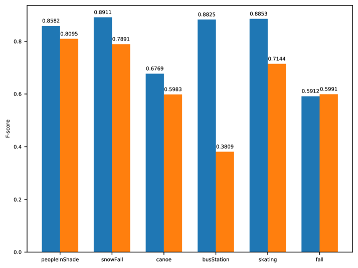
Figure 8: The F1 score obtained by our proposed approach in scenes from ’peopleInShade’, ’snowFall’, ’canoe’, ’busStation’, ’skating’, fall. The blue bar on the chart represents the results presented by the best equations discovered during the mutation process, while the orange bar represents the result obtained by the best equations discovered in unseen scenes. Observe that while the F1 score has decreased for most scenes in unseen sequences (orange bar), the best LBP equations are still adequate to deal with unseen sequences over time. In contrast, the F1 score dropped dramatically from 0.8825 %, to 0.3809 % for the ’busStation’ scene.

We also evaluate the best LBP equations discovered by our algorithm in unseen sequences. Therefore, we selected around 100 $\sim$ 150 sequences for each scene. The results are shown in Figure 8. From the chart, we can see that although the F1 score has decreased for most scenes in unseen sequences (orange bar), the best LBP equations are still adequate to deal with unseen sequences over time. In contrast, the F1 score dropped drastically from 0.8825 %, to 0.3809 % for the ’busStation’ scene. The best LBP equation discovered by our algorithm does not seem to be adequate for ’busStation’ scene over time. To help us understanding the performance of the ’busStation’ scene, we performed a new experiment adding 27 more new sequences during the mutation process and our algorithm discovered a new best equation: $(Z/C)/(Z/C)/(Z*(Z/C)-(Z+C))-a$. When applying this better equation to unseen sequences, it seems to deal better with the challenges presented in the ’busStation’ scene by increasing the F1 score from 0.3809% to 0.4483%.

In general, we can see that the proposed framework is capable of finding useful LBP equations to deal with different challenges encountered in a given scene. Although one scene has similar challenges to the other, our experiments showed that the best equation for dealing with them will not be the same, since each one is unique and the dynamics of the scene also contributes to the choice of the best equation. This can be noticed by the couples of scenes [’peopleInShade’ and ’busStation’], [’canoe’ and ’fall’] and [’snowFall’ and ’skating’] that have similar challenges and yet the best equation found out for each of them by our approach is different (see Table 2). Furthermore, when performing experiments in unseen sequences, we can see that the best LBP equation that seemed to be adequate to deal with the ’busStation’ scene initially does not seem to be appropriate over time. By increasing the number of sequences during the mutation process, a new better equation was discovered indicating that the number of sequences used in the mutation process can impact the performance of our framework.

Finding a specific equation for a given scene manually is a laborious task that requires a in-depth knowledge of the scene and a trial-error process by experts. The approach presented in this paper can be very useful saving human research time. Finally, the best mathematical LBP equations found out in this work may be different for the same scene, especially if a different background subtraction method is used or our approach is applied to another type of domain. In addition, the results presented in this paper are an non-exhaustive search for the best LBP, due to limited computational resources. Therefore, the approach presented in this paper is especially ideal for discovering the best mathematical equations for solving specific problem in computer vision field.

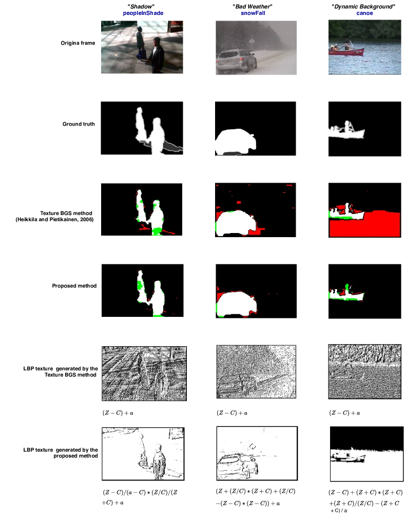
Figure 6: Background subtraction results using the CDnet-2014 data set. From top to bottom: (a) Original frame, (b) Ground truth, (c) Texture BGS method, (d) Proposed method, and (e) LBP texture. The true positives (TP) pixels are in white, the true negatives (TN) pixels are in black, the false positives (FP) pixels are in red, and the false negatives (FN) pixels are in green.

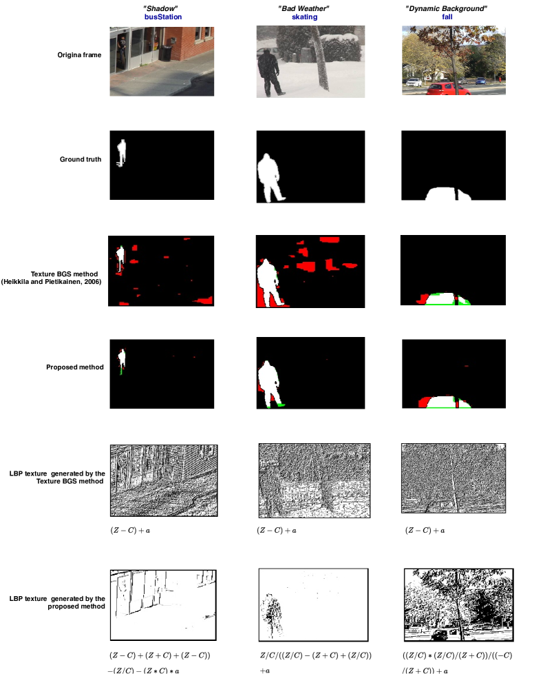
Figure 7: Background subtraction results using the CDnet-2014 data set. From top to bottom: (a) Original frame, (b) Ground truth, (c) Texture BGS method, (d) Proposed method, and (e) LBP texture. The true positives (TP) pixels are in white, the true negatives (TN) pixels are in black, the false positives (FP) pixels are in red, and the false negatives (FN) pixels are in green.

Videos	Challenge	LBP structure	Best LBP equation
peopleInShade	Consists of pedestrian walking outdoor. The main challenges are: hard shadow cast on the ground by the walking persons and illumination changes.	(Z o C) o (a o C) o (Z o C) o (Z o C) o a	(Z - C) / (a - C) * (Z / C) / (Z + C) + a
snowFall	Contains a traffic scene in a blizzard. The main challenges are: low-visibility winter storm conditions, snow accumulation, the dark tire tracks left in the snow.	(Z o (Z o C) o (Z o C) o (Z o C) o (Z o C) o (Z o C)) o a	(Z +( Z / C) * (Z + C) + (Z / C) - (Z - C) * (Z - C)) + a
canoe	Shows people in a boat with strong background motion. The main challenges are: outdoor scenes with strong background motion.	(Z o C) o (Z o C) o (Z o C) o (Z o C) o (Z o C) o (Z o C o C) o a	(Z - C) + (Z + C) * (Z + C) + (Z + C) / (Z / C) - (Z + C + C) / a
busStation	Presents people waiting in a bus station. The main challenges are: hard shadow cast on the ground by the walking persons.	(Z o C) o (Z o C) o (Z o C) o (Z o C) o (Z o C) o a	(Z - C) + (Z + C) + (Z - C) - (Z / C) - (Z * C) * a
skating	Shows people skating in the snow. The main challenges are: low-visibility winter storm conditions and snow accumulation.	Z o C o ((Z o C) o (Z o C) o (Z o C)) o a	Z / C/ ((Z / C) - (Z + C) +(Z / C)) + a
fall	Show cars passing next to a fountain. The main challenges are: outdoor scenes with strong background motion.	((Z o C) o (Z o C) o (Z o C)) o ((o C) o (Z o C)) o a	((Z / C) * (Z / C) / (Z + C)) / ((-C) / (Z + C)) + a

Table 2: List of the best equations for dealing with different challenges encountered in real-world scenarios. From the left to the right: (a) different types of scenes, (b) with their main challenge descriptions, (c) the best LBP structure, and (d) the best LBP equation.

Videos	Method	Precision	Recall	F-score
peopleInShade	Texture BGS	0.7339	0.9009	0.8088
	Proposed approach	0.8211	0.8988	0.8582
snowFall	Texture BGS	0.5970	0.9384	0.7298
	Proposed approach	0.8673	0.91638	0.8911
canoe	Texture BGS	0.1106	0.8183	0.1949
	Proposed approach	0.8710	0.5535	0.6769
busStation	Texture BGS	0.2747	0.9695	0.4282
	Proposed approach	0.8792	0.8859	0.8825
skating	Texture BGS	0.2666	0.9161	0.4130
	Proposed approach	0.9213	0.8520	0.8853
fall	Texture BGS	0.5453	0.7904	0.6453
	Proposed approach	0.4625	0.8190	0.5912

Table 3: Performance using the CDnet-2014 data set.

5 Conclusion

In this paper, we present a novel framework for discovering the appropriate Local Binary Patterns to deal with the main challenges encountered in real-world scenarios. The proposed framework can reduce human bias and time by proposing a search space designed by a generative network instead of hand-designed features. In addition, it can discover equations that we may never have thought of yet. Experimental results in video sequences show the potential of the proposed approach and its effectiveness in discovering the best equation for dealing with the problems found in a particular complex scene. Future work includes formulating new structures of equations other than LBP and carrying on experiments on scenes with different challenges. Moreover, the method developed in this paper could be extended to neural architecture search. This could be done by generating and combining basic mathematical structures as building blocks, enabling the construction of a variety of neural architectures.

References

- Alzaidi and Kazakov (2011) A. Alzaidi and D. Kazakov. Equation discovery for financial forecasting in the context of islamic banking. In IASTED International Conference on Artificial Intelligence and Applications (AIA), 2011.
- Bahdanau et al. (2015) D. Bahdanau, K. Cho, and Y. Bengio. Neural machine translation by jointly learning to align and translate. In International Conference on Learning Representations (ICLR), 2015.
- Bergstra and Bengio (2012) J. Bergstra and Y. Bengio. Random search for hyper-parameter optimization. Journal of Machine Learning Research (JMLR), 13:281–305, 2012.
- Bisiani (1992) R. Bisiani. Beam search. Encyclopedia of Artficial Intelligence, pages 1467–1468, 1992.
- Bukhari et al. (2017) D. Bukhari, Y. Wang, and H. Wang. Multilingual convolutional, long short-term memory, deep neural networks for low resource speech recognition. Procedia Computer Science, 107:842–3847, 2017.
- Chen et al. (2004) P-W. Chen, J-Y. Wang, and H-M. Lee. Model selection of SVMs using GA approach. In IEEE International Joint Conference on Neural Networks (IJCNN), 2004.
- Cho et al. (2014) K. Cho, B. van Merrienboer, C. Gulcehre, D. Bahdanau, F. Bougares, H. Schwenk, and Y. Bengio. Learning phrase representations using rnn encoder-decoder for statistical machine translation. In Proceedings of the Empiricial Methods in Natural Language Processing (EMNLP), pages 1724–1734, 2014.
- Dahl et al. (2013) G. Dahl, T. Sainath, and G. Hinton. Improving deep neural networks for LVCSR using rectified linear units and dropout. In IEEE International Conference on Acoustics, Speech, and Signal Processing (ICASSP), 2013.
- Deng et al. (2009) J. Deng, W. Dong, R. Socher, L.-J. Li, K. Li, and L. Fei-Fei. Imagenet: A large-scale hierarchical image database. In IEEE Conference on Computer Vision and Pattern Recognition (CVPR), 2009.
- Dimensions (2021) Dimensions. Digital Science & Research Solutions In, 2021. URL https://www.dimensions.ai. Accessed on 28.02.2021.
- Drori et al. (2018) I. Drori, Y. Krishnamurthy, R. Rampin, R. Lourenco, J. Ono, K. Cho, C. Silva, and J. Freire. AlphaD3M: Machine learning pipeline synthesis. In International Workshop on Automated Machine Learning, 2018.