ScaleFreeCTR: MixCache-based Distributed Training System for CTR Models with Huge Embedding Table

Abstract.

Because of the superior feature representation ability of deep learning, various deep Click-Through Rate (CTR) models are deployed in the commercial systems by industrial companies. To achieve better performance, it is necessary to train the deep CTR models on huge volume of training data efficiently, which makes speeding up the training process an essential problem. Different from the models with dense training data, the training data for CTR models is usually high-dimensional and sparse. To transform the high-dimensional sparse input into low-dimensional dense real-value vectors, almost all deep CTR models adopt the embedding layer, which easily reaches hundreds of GB or even TB. Since a single GPU cannot afford to accommodate all the embedding parameters, when performing distributed training, it is not reasonable to conduct the data-parallelism only. Therefore, existing distributed training platforms for recommendation adopt model-parallelism. Specifically, they use CPU (Host) memory of servers to maintain and update the embedding parameters and utilize GPU worker to conduct forward and backward computations. Unfortunately, these platforms suffer from two bottlenecks: (1) the latency of pull & push operations between Host and GPU; (2) parameters update and synchronization in the CPU servers. To address such bottlenecks, in this paper, we propose the ScaleFreeCTR: a MixCache-based distributed training system for CTR models. Specifically, in SFCTR, we also store huge embedding table in CPU but utilize GPU instead of CPU to conduct embedding synchronization efficiently. To reduce the latency of data transfer between both GPU-Host and GPU-GPU, the MixCache mechanism and Virtual Sparse Id operation are proposed. Comprehensive experiments are conducted to demonstrate the effectiveness and efficiency of SFCTR. In addition, our system will be open-source based on MindSpore in the near future.

1. Introduction

To alleviate the problem of information explosion, recommender systems are widely deployed to provide personalized information filtering in online information services, such as web search, news recommendation, and online advertising. In recommender systems, Click-Through Rate (CTR) prediction is a crucial task, which is to estimate the probability that a user will click on a recommended item under a specific context, so that recommendation decisions can be made based on the predicted CTR values (McMahan et al., 2013; Zhou et al., 2018; Cheng et al., 2016; Guo et al., 2017; Zhao et al., 2020; He et al., 2014). Due to the superior performance of feature representation in computer vision (He et al., 2016) and natural language processing (Devlin et al., 2019), deep learning techniques attract the attention of recommendation community. Therefore, industrial companies propose various deep CTR models and deploy them in their commercial systems, such as Wide & Deep (Cheng et al., 2016) in Google Play, DeepFM (Guo et al., 2017) in Huawei AppGallery and DIN (Zhou et al., 2018) in Taobao.

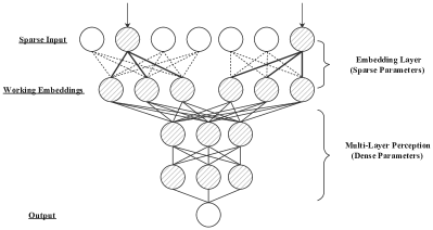
Figure 1. Embedding & MLP paradigm of CTR models.

To achieve good performance, deep CTR models with complicated network architectures need to be trained on huge volume of training data  for several epochs, leading to low training efficiency. Such low training efficiency (namely, long training time) may result in performance degradation when the model is not produced on time and therefore delayed to deploy (Wang et al., 2020). Hence, how to improve training efficiency of deep CTR models without hurting model performance is an essential problem in industrial recommender systems. Incremental learning (Wang et al., 2020; Xu et al., 2020; Yang et al., 2019) and distributed training (Jiang et al., 2019; Rong et al., 2020; Zhao et al., 2020) are two common paradigms to tackle this problem from different perspectives. Incremental learning is a complement to batch training, which only utilizes the most recent data to update the model. Distributed training utilizes extra computational resources to speed up batch training process.

Many applications, such as computational finance (Heaton et al., 2016), computer vision (You et al., 2018) and natural language processing (Brown et al., 2020), also need training datasets of billions of instances with TB size. To perform distributed training on these applications, data-parallelism, such as the All-Reduce based approach (Sergeev and Balso, 2018; Mamidala et al., 2004), is usually adopted, as the models in such applications are small enough to put in the High Bandwidth Memory (HBM) of a single GPU device (usually no more than 32 GB). However, different from the above mentioned applications with dense training data, the data of recommendation and advertising is high-dimensional and sparse (Guo et al., 2018; Ying et al., 2018; Cheng et al., 2016). As shown in Figure 1, existing deep CTR models follow the Embedding & Multi-Layer Perception (MLP) paradigm. The embedding layer transforms the high-dimensional sparse input into low-dimensional dense real-value vectors (Zhang et al., 2016). The sparse features can easily reach a scale of several billions or even trillions (Zhao et al., 2020), making the parameter size of the embedding layer to be hundreds of GB or even TB, which is significantly larger than the HBM of a single GPU device with several orders of magnitude. Therefore, when performing distributed training, it is not a reasonable solution to conduct data-parallelism only, since a single GPU cannot always afford to accommodate all the embedding parameters. Due to this reason, the majority of the existing distributed training frameworks for recommendation consider model-parallelism.

Limitations of Existing Model-Parallelism Solutions for Recommendation Models. As a classic distributed training framework, Parameter Server (PS) (Li et al., 2014; Jiang et al., 2019; Kim et al., 2019) is widely used to train CTR models with large amount of embedding parameters. Two distinguished roles, namely server and worker, exist in PS mechanism, as shown in Figure 2. The servers maintain and synchronize model parameters, and the workers perform the forward and backward computations. Specifically, a worker pulls its corresponding parameters from the severs, conducts forward computation to make predictions, computes gradients by back-propagation and finally pushes such gradients to the servers. Deployed in the cluster of high performance devices , the computation of recommendation models in workers is very fast and therefore the efficiency of traditional PS usually suffers from these two bottlenecks: (1) pull and push operation between the servers and the workers; (2) parameters synchronization in the servers after receiving gradients from the workers.

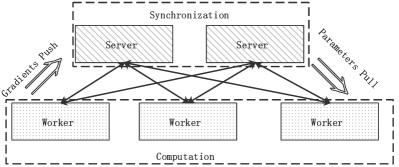
Figure 2. The training process of parameter server.

To make full use of powerful computation ability and high-speed bandwidth of GPUs, various distributed training systems for deep CTR models are proposed by industrial companies, such as HugeCTR  by NVIDIA, DLRM (Naumov et al., 2019) by Facebook, DES (Rong et al., 2020) by Tencent and HierPS (Zhao et al., 2020) by Baidu. HugeCTR and DLRM devide the parameters of the embedding layer into multiple pieces such that each piece can be stored in the HBM of a single GPU. Due to the limited size of HBM (normally less than 32 GB), we need tens or even hundreds of GPUs to store the embedding parameters, which is expensive. Therefore, the solutions provided by HugeCTR and DLRM are impractical to train deep CTR models with huge embedding table.

To overcome this limitation, DES and HierPS utilize the Host memory to maintain the embedding parameters of large size. More specifically, DES proposes a field-aware partition strategy to reduce communication data among GPUs, while the communication cost between Host-GPUs are not considered to optimize. HierPS introduces a Big-Batch Strategy to cache the working parameters in GPUs to decrease the latency of parameters/gradients transfer between Host-GPUs, but the latency between two such consecutive Big-Batches is not tolerable. Therefore, both of DES and HierPS still suffer from the latency of parameters/gradients transfer between Host-GPUs.

Challenges & contributions. From the above observations, we can see that there are two challenges when designing a distributed training framework for deep CTR models. First, how to reduce the latency of parameters/gradients transfer between Host-GPUs is a key factor, as a large latency leads to low scalability. Second, how to reduce the amount of parameters/gradients transfer between Host-GPUs and GPU-GPU is also important.

There are two distinguishable characterizations for data in recommendation, which help us to design a distributed training system for deep CTR models and tackle the above mentioned challenges. First, working parameters are of small size. Working parameters refer to all the parameters that exist and will be updated in the current batch of training data, including the embedding parameters of all the existing sparse features in the current batch and parameters in MLP. Sparse features existed in the current batch are not many and the parameters in MLP are also limited, which lead to small size of working parameters. Second, sparse features follow power-law distribution. That is to say, a very small portion of the sparse features appear in the dataset with high frequencies, which also suggests that there exist many duplicate features in a batch of training data. The first characterization gives the chance to eliminate the latency between Host-GPUs by utilizing the cache mechanism, and the second characterization provides us the opportunity to reduce the amount of parameters/gradients transfer between both Host-GPUs and GPU-GPU by re-organizing the data in the current batch.

Leveraging the characterizations of small size of working parameters and power-law distribution of features, we propose ScaleFreeCTR (SFCTR for short), to training deep CTR models with huge size of embedding parameters efficiently, in a distributed GPU cluster. SFCTR consists of three modules, i.e., Data-Loader, Host-Manager and GPU-Worker. These three modules in SFCTR make the following contributions:

• SFCTR utilizes Host memory to maintain the huge embedding table and GPU to conduct the synchronization of embedding parameters efficiently. To reduce the amount of parameters/gradients transfer between Host-GPUs and GPU-GPU, a Virtual Sparse Id (VSI) operation is proposed in Data-Loader of SFCTR, removing the duplicate feature embeddings in a batch of data.

• To eliminate the latency of parameters/gradients transfer between Host-GPUs, we propose MixCache, an efficient cache mechanism, in Host-Manager of SFCTR to store the working parameters in GPUs.

• A three-stage pipeline, that overlaps Data-Loader, Host-Manager, and the training in GPU-Worker, is proposed to match the inevitable GPU computation.

• Comprehensive experiments are conducted on a public benchmark dataset to demonstrate the efficiency of SFCTR, which is 6.9X faster than HugeCTR by NVIDIA and 1.3X faster than the optimized parameter server of MxNet. Ablation studies are also performed to validate the effectiveness and efficiency of VSI operation, MixCache mechanism and three-stage pipeline.

2. Related Work and Background

In this section, we discuss related literature of deep CTR models and distributed training platforms for deep CTR models.

2.1. Deep CTR Models

CTR prediction models evolves from logistic regression (McMahan et al., 2013), factorization machines and its variants (Rendle, 2010; Juan et al., 2016), to deep learning models (Guo et al., 2017; Cheng et al., 2016; Liu et al., 2019; Huang et al., 2019; Wang et al., 2017; Liu et al., 2020; Guo et al., 2019). Generalized Logistic Regression (LR) models, such as FTRL (McMahan et al., 2013), are widely used in recommender systems, because of their robustness and efficiency. Recently, due to superior performance of feature representation in computer vision and natural language processing, deep learning techniques attracts more attention in recommendation community. Most deep CTR models follow the Embedding & MLP paradigm, as presented in Figure 1. The embedding layer transforms the high-dimensional sparse input (which are usually categorical features, such as city, gender, user id) into low-dimensional dense real-value vectors. MLP layers aim to learn the non-linear interactions among features, such as DeepFM (Guo et al., 2017), xDeepFM (Lian et al., 2018), DIN (Zhou et al., 2018).

Why deep CTR models are of large size. As stated earlier, all the features that serve as input for deep CTR models are assumed to be in categorical form, therefore they have to be encoded into real-value to apply gradient-based optimization methods. One-hot encoding is an approach to encode a categorical feature into a sparse binary vector, which all bits are 0’s except for just one bit being 1. For example, the one-hot encoding of a categorical feature with index $i$ is $s_{i}=(0,0,...,1,...,0)^{T}\in\mathbb{R}^{n}$, where $n$ is the number of features in all. The $i$-th of $s_{i}$ is 1 while other bits are 0’s. If followed up a matrix multiplication, we have a low-dimensional representation of the categorical features. That is to say, given a dense matrix $E\in\mathbb{R}^{n\times m}$, $s_{i}^{T}\times E$ is the $m$-dimensional dense real-value vector for feature with index $i$. In this way, a categorical feature is transformed into a low-dimensional dense vector.

However, due to the fact that there are often billions or even trillions of categorical features (i.e., $n$ is very large), the one-hot vector can be extremely high-dimensional. Therefore nowadays it is more usual to use the look-up embedding as a mathematically equivalent alternative. For instance, for the feature with index $i$, it directly looks up the $i$-th row from the dense matrix $E$. The matrix $E$ is often referred to as embedding table. As $n$ is usually very huge (in billion- or trillion-scale), the size of embedding table may take hundreds of GB or even TB to hold. Whereas, the parameter size in MLP is relatively much smaller. Therefore, deep CTR models with large embedding table are of large size, and the parameters in the embedding table take the majority of the model size.

2.2. Distributed Training Platforms for Deep CTR Models

Investigating advance parallel mechanism among the workers and servers in distributed training systems is important (Li et al., 2014). Distributed training process includes two main phases, namely, computation and parameter synchronization. In computation phase, the loss and gradients of parameters are computed according the input data (including both features and labels) in workers. In the synchronization phase, the gradients are collected and adopted to update the maintained parameters by servers. As summarized in  (Zhao et al., 2020), there are three typical synchronization patterns: (1) Bulk Synchronous Parallel (BSP) (Valiant, 1990), which strictly synchronizes updates from all the workers; (2) Stale Synchronous Parallel (SSP) (Ho et al., 2013), which synchronizes results from faster workers; (3) Asynchronous Parallel (ASP), which does not require any synchronization on the gradients from different workers. Although ASP and SSP improves training efficiency by reducing synchronization frequency, they suffer from degrading model performance (such as accuracy, convergence rate) (Gupta et al., 2016). Aiming to not sacrificing model performance, we focus on comparing the existing distributed training systems with BSP. Our proposed SFCTR is also working with BSP.

We compare the existing distributed training systems for deep CTR models with BSP. To improve the inferior performance of distributed training in Tensorflow (Abadi et al., 2016), MxNet (Chen et al., 2015) and Pytorch (Lerer et al., 2019), both Horovod (Sergeev and Balso, 2018) and BytePS (Peng et al., 2019) are proposed to support different platforms. Horovod speeds up the training of dense models based on its efficient and elegant implementation of Ring-AllReduce mechanism. BytePS further improves synchronizing parameters in different layers by prioritized scheduling, i.e., optimizing the order of different layers to synchronize parameters during the backward-propagation and the forward-computation phase. Recently, to training deep CTR models with a large embedding table, various systems are proposed, such as HugeCTR ⁵, DLRM (Naumov et al., 2019), DES (Rong et al., 2020) and HierPS (Zhao et al., 2020). The comparison of SFCTR with the most relevant platforms are summarized in Table 1.

Relationship with related work: First, HugeCTR and DLRM do not design to hold embedding table in the Host memory, therefore models with very large embedding tables (hundreds of GB or TB) are not supported. Second, as DES, HierPS and SFCTR support storing embedding in Host, the latency of parameters/gradients transfer between Host-GPUs raises an issue. DES does not specifically optimize the latency between Host-GPUs. HierPS adopts the Big-Batch strategy to reduce such latency, but there still exists intolerable latency between such two consecutive Big-Batches. To eliminate this latency, SFCTR is equipped with the MixCache, an efficient cache mechanism, to store the working parameters in GPUs, such that much parameters/gradients transfer between Host-GPUs can be avoided.

Table 1. The comparison between different approaches.

	Embedding	Host-GPUs
	in Host	Latency
HugeCTR	$\times$	Not Involve
DLRM	$\times$	Not Involve
DES	$\surd$	Large
HierPS	$\surd$	Small
SFCTR	$\surd$	Hiding

3. Overview of ScaleFreeCTR

Algorithm 1 The workflow of ScaleFreeCTR.

1:while not converge do

2:     batch $\leftarrow$ get_batch();

3:     global_id, virtual_id $\leftarrow$ virtual_sparse_id(batch);

4:     working, noworking $\leftarrow$ manager_get(global_id);

5:     push_parameters_to_cache(working);

6:     pull_parameters_to_host(noworking);

7:     mini_batches, local_id $\leftarrow$ shard(global_id, virtual_id);

8:     for  $i\in[1,\#GPU]$ do

9:         common_embed $\leftarrow$ gather_cache(local_id);

10:         common_embed = AllReduce(common_embed);

11:         batch_embed_i $\leftarrow$ gather(global_embed, mini_batch_i);

12:         grad_i $\leftarrow$ forward_backward(loss_i);

13:         grad_i $\leftarrow$ grad_synchronize(grad_i);

14:         update_sparse(grad_i);      

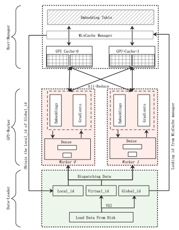
Figure 3. The architecture of ScaleFreeCTR, including Data-Loader (line 2-3 in Aglorithm 1, as presented in Section 4), Host-Manager (line 4-7 in Aglorithm 1, as elaborated in Section 5) and GPU-Worker (line 9-14 in Aglorithm 1, as described in Section 6).

In this section, we overview the architecture and workflow of SFCTR in high-level. As presented in Figure 3, SFCTR consists of three modules, i.e., Data-Loader, Host-Manager and GPU-Worker (the details are presented in Section 4, Section 5 and Section 6, respectively). At first, we introduce the workflow of SFCTR according to Aglorithm 1.

• The line 2-3 in Aglorithm 1 is the Data-Loader, which is responsible for loading data from disk to main memory. To reduce the amount of parameters/gradients transfer between Host-GPUs and GPU-GPU, a Virtual Sparse Id (VSI) operation is proposed. To construct a uniform representation of the working embedding parameters in the current batch, VSI operation removes duplicated feature ids in a batch of data and keeps only one copy of feature ids which is indexed by global_id. For each instance in the current batch, VSI represents a feature by virtual_id, which serves as a pointer to find the corresponding global_id (line 3).

• The Host-Manager (line 4-7 in Aglorithm 1) maintains embedding parameters in Host memory and transfers the working embedding parameters in a batch of data from Host to the corresponding GPUs. To eliminate such latency of parameters/gradients transfer between Host-GPUs, we propose MixCache, an efficient cache mechanism in the Host-Manager to store the working parameters in GPUs. MixCache allocates a cache buffer for each GPU, and stores working embedding parameters in each of such cache buffers in a non-overlap manner. MixCache also functions to update cache buffers. More specifically, MixCache checks which embedding parameters are needed for the next batch (referred as working in line 4), and predicts which embedding parameters are not needed for a short future (referred as noworking in line 4). MixCache pushes the working from Host to cache buffers (line 5) and pulls noworking from cache buffers to Host if the cache buffers are full (line 6). Next, Host-Manager dispatches training data to individual GPUs, and identifies local_id of each feature in the local GPU (line 7).

• The GPU-Worker completes the training process in GPUs, including embedding table lookup (line 9-11), forward prediction and backward gradients computation (line 12), MLP parameters and working embedding parameters updating (line 13-14). Host-Manager and GPU-Worker act in producer-consumer fashion, namely, Host Manager prepares embedding parameters of a batch of data while GPU-Worker consumes the batch of data and updates parameters.

Three-stage pipeline:

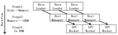
Figure 4. The three-stage pipeline.

As presented in Figure 4, a three-stage pipeline is applied to overlap timeline of different modules in SFCTR using multi-thread technologies. The training process involves three stages: (1) Data-Loader loads data and removes duplicated feature embeddings by keeping global_id and virtual_id; (2) Host-Manager pushes the working embedding parameters to the cache buffers of GPUs and pulls the unnecessary embedding parameters to Host; (3) GPU-Worker performs forward/backward calculation and conducts communication on GPUs. The hardware resources needed in the three stages are different: namely, Disk, CPU and GPU, respectively. Therefore, such different hardware resources can be fully utilized, if jobs of these three stages are scheduled to three different thread pools reasonably. The Host-Manager thread receives global batches of data from the Data-Loader thread and pushes the processed data/parameters to the GPU-Worker thread, as illustrated in Figure 4. When the GPU-Workers are busy with training on the current batch of data, the Data-Loader thread is loading data and the Host-Manager thread is preparing parameters in cache buffers from the next batch. Therefore, once the training on the current batch is finished, the required embedding parameters of the next batch are already in HBM of GPUs, so that the training on the next batch can be started immediately.

4. Data-Loader

The Data-Loader reads batches of training data from disk to Host memory. In datasets for CTR prediction problem, there exist many repeated features across different data samples in batches. Such redundancy brings unnecessary overhead on parameters/gradients transfer between Host-GPUs in Host-Manager and between GPU-GPU in GPU-Worker. To reduce such redundancy, we propose a Virtual Sparse Id (VSI) operation in Data-Loader. To construct a uniform representation of the working embedding parameters in the current batches, VSI operation removes duplicate feature embeddings in a batch of data and keeps only one copy of feature embeddings which are indexed by global_id. For each instance in the current batch, VSI represents a feature by virtual_id, which serves as a pointer to find the corresponding global_id.

Example for the VSI operation in Data-Loader: There is a batch with two instances: $\{[1,3,2],[2,3,1]\}$, where each number represents a feature index. After eliminating duplicate features, VSI operation keeps their global_id, sorted by the order of appearance, as $(1,3,2)$. VSI operation represents the two data instances as $\{[0,1,2],[2,1,0]\}$, where each number is a virtual_id. $\texttt{virtual\_id}=0$ retrieves the global_id with index 0, which is $\texttt{global\_id}=1$. As we can see, utilizing global_id and virtual_id is able to recover the data with duplicate feature embeddings.

As we will see later, working embedding parameters are distributed stored in the cache buffers across GPUs, therefore training model on one GPU may need embedding parameters in other GPUs. Loading the batches that are trained cross all the GPUs (referred to as “global batches”) to the current GPU is helpful to construct a uniform representation of working embedding parameters. Such a uniform representation introduces a more efficient GPU-GPU communication scheme, which is detailed in Section 6. The size of such uniform representation for working embedding parameters is much less when we use global_id instead of original feature index. In the above example, the size of this uniform representation is halved if we use global_id, because in the original format there are six feature embeddings while three of them are duplicate and therefore eliminated. To summarize, VSI operation helps construct a more space-efficient uniform representation of working embedding parameters, and therefore reduces the amount of parameters/gradients transfer between GPU-GPU. As will be discussed in Section 5, the amount of transfer between Host-GPUs is also optimized by VSI operation.

5. Host-Manager

Host-Manager maintains embedding parameters in Host memory and transfers the working embedding parameters in a batch of data from Host to GPUs. To eliminate the latency of parameters/gradients transfer between Host-GPUs, MixCache, which is an efficient cache mechanism in Host-Manager, is proposed. MixCache allocates a cache buffer in HBM of each GPU, which stores the working embedding parameters for the next batch of training data in the corresponding GPU. MixCache utilizes a hash function (such as modulo hashing) to divide the features into disjointed groups such that each cache buffer in a GPU is responsible for one such group.

Each cache buffer of a GPU stores working embedding parameters, of which the corresponding features are in its responsibility. As shown in the three-stage pipeline in Section 3, MixCache identifies the working embedding parameters in the next batch of data and transfers them from Host to the cache buffer if they are not in the cache buffer for now, when the current batch of data is trained in GPU. Therefore, when the training of the current batch is finished, GPUs do not need to wait the working embedding parameters to be transferred and can train the next batch without any latency. As can be seen, embedding parameters of a working feature are transferred to cache buffer at most once with VSI operation performed beforehand; otherwise, embedding parameters of a working feature are repeatedly transferred to cache buffer if this feature is duplicated in the next batch. That is to say, VSI operation reduces the amount of parameters/gradient transfer between Host-GPUs, which has been stated in Section 4.

As the cache buffer is of limited size, embedding parameters have to be transferred back to Host if the cache buffer is full and new working embedding parameters of next batches are needed to transfer into the cache buffer. Embedding parameters of a feature can be transferred back to Host under two conditions that have to be satisfied both: first, the embedding parameters of this feature finish updating; second, this feature does not exist in the next batches that we consider. The first condition guarantees the updating of embedding parameters not interrupted by parameters transfer. The second condition prevents the overhead cost by transferring embedding parameters of a feature to the cache buffer immediately after pulling it out.

Example for the MixCache in Host-Manager:

• Current features maintained in cache: Assume the buffer size of GPU cache is $12$ and the following features’ embedding parameters are maintained in the cache: $[1,3,2,5,4,6,$ $12,13,14,15,9]$, where is only one slot available.

• The features which will be used in next batch: Three features (with $\texttt{global\_id}=6,7,8$) in the next batch need to be transferred in the cache buffer, where exists only one slot.

• Removing and transferring: Assume features with $\texttt{global\_id}=3,2,5,4$ are used in current batch and do not finish updating, therefore they are not candidates for removal. Feature with $\texttt{global\_id}=6$ is not reasonable to be removed from the cache buffer, as it is needed in the next batch. As a result, features with $\texttt{global\_id}=1$ is selected to be replaced by features with $\texttt{global\_id}=7$, feature with $\texttt{global\_id}=8$ is positioned in the available slot, and feature with $\texttt{global\_id}=6$ is untouched. Now, the following features’ embedding parameters are maintained in the cache: $[7,3,2,5,4,6,12,13,14,15,9,8]$

6. GPU-Worker Training

As the embedding parameters in the current training batch may be located in different GPUs, both the embedding parameters in the forward phase and the gradients in the backward phase need to be synchronized across different GPUs.

6.1. Forward

When synchronizing embedding parameters in the forward phase, every GPU collects the embedding parameters in all GPUs for the current batches of training data. We choose to adopt all-reduce communication scheme, where every GPU only needs to communicate twice with another two GPUs. To realize the all-reduce communication scheme, a uniform representation of embedding parameters indexed by global_id is needed in every GPU, which is referred to as Local Common Embedding in Figure 5.

Example of the forward phase in GPU-Worker: Consistent with the example in Section 4, a global batch of two data instances $\{[1,3,2],[2,3,1]\}$ load for training, where the first instance feeds in Worker-0 and the second one feeds in Worker-1. These two workers know all the global_id ($(1,3,2)$ in this example) in the current global batch of data, realized by Data-Loader, as shown in Figure 5:

• Gather in Worker-0: its cache buffer stores $e_{1}$, $e_{3}$ and other embeddings, hence, the Local Common Embedding of the current global batch in Worker-0 is $(e_{1},e_{3},0)$ ($e_{2}$ is not in Worker-0 so the position of global_id 2 is presented with 0 value).

• Gather in Worker-1: similarly, the Local Common Embedding of Worker-1 is $(0,0,e_{2})$. As the format of the Local Common Embedding is consistent across the workers, all-reduce communication scheme is possible to perform, so that both workers keep the same embedding parameters that are appeared in the current global batch, known as Global Common Embedding in Figure 5.

• All-reduce: utilizing virtual_id of each feature, the original training data with feature embeddings are recovered, as $[e_{1},e_{3},e_{2}]$ in Worker-0 and $[e_{2},e_{3},e_{1}]$ in Worker-1.

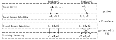
Figure 5. Synchronization of embedding in forward phase.

6.2. Backward

After backward propagation, the gradients of all the embedding parameters are computed in different workers, known as Local Gradients in Figure 6. Then virtual_id is utilized to transform Local Gradients to Local Common Gradients to keep a uniform order, i.e, the same as in Local Common Embedding in Figure 5. This transformation is known as unsorted_segment_sum in Tensorflow. For example in Figure 6, the Local Gradients $(g_{1},g_{3},g_{2})$ and $(g_{2},g_{3},g_{1})$ are accumulated as Local Common Gradients $(g_{1},g_{3},g_{2})$ and $(g_{1},g_{3},g_{2})$ by worker-0 and worker-1 respectively.

After this transformation, the format of the Local Common Gradients is consistent across the workers. So all-reduce communication scheme is possible to perform to collect the Local Common Gradients of the other GPUs, and the Global Common Gradients are computed by summing such local ones. Finally, each worker uses Global Common Gradients to update the embedding parameters stored in its Cache Buffer. For example, based on the Global Common Gradients, worker-0 updates $e_{1},e_{3}$ and worker-1 updates $e_{2}$.

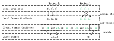
Figure 6. Synchronization and updating of gradients in backward phase.

7. Experiment

In this section, we conduct extensive experiments to answer the following research questions:

• RQ1: How does SFCTR perform compared to other distributed training systems for CTR prediction task?

• RQ2: Can VSI operation reduce the amount of communication data and accelerate the training process?

• RQ3: Can MixCache mechanism eliminate the latency between Host-GPU without sacrificing the model accuracy?

• RQ4: How does the proposed 3-stage pipeline improve the efficiency of SFCTR?

7.1. Setting

7.1.1. Environment

To realize all-reduce communication scheme efficiently, our GPU cluster is connected through InfiniBand which is a high-speed, low latency, low CPU overhead network hardware. Based on InfiniBand network, Remote Direct Memory Access (RDMA) technology is applied to speed-up GPU communication. Specifically, we evaluate SFCTR on a cluster with four GPU servers connected by a 100Gb RDMA network adaptor. Each server has 2 Intel Xeon Gold-5118 CPUs with 18 cores (36 threads), 8 Tesla V100 GPUs with 32 GB HBM, and approximate 1 TB Host memory. The GPUs in each server are connected with PCIe.

7.1.2. Dataset

To make it easy for audiences to reproduce the experiments, we adopt a large-scale real-world public available dataset Criteo-TB  to conduct our experiments and verify the performance of SFCTR. It consists of 24 days consecutive user click logs from Criteo, including 26 categorical features and 13 numerical features. The first column of the dataset is the label indicating whether the ad has been clicked or not.

To investigate the performance of SFCTR to handle different sizes of embedding table, we construct two versions of Criteo-TB, namely 10 GB and 100 GB, through different thresholds (the thresholds of 10 GB and 100 GB are 10 and 1, respectively) to filter low-frequency features (similar to (Qu et al., 2019)). Specifically, the 10 GB (100 GB) contains 33 (330) million features with the size of embedding table $33~{}(330)~{}M\times 4~{}B\times 80~{}\approx~{}10~{}(100)~{}GB$, where $4~{}B$ indicates the data type of parameters as float32, $80$ indicates the embedding size. Since we adopt the widely-used Adam as the optimizer, which needs to maintain another two corresponding variables (namely, momentum and velocity), the size of training parameters is three times of the embedding size. Therefore, the parameter size is 300 GB when the embedding table is 100 GB, which is larger than $8\times 32~{}GB$ (HBMs of 8 GPUs) and can not be put in GPU memory directly.

7.1.3. Base Model & Metric

We use the widely-used DeepFM (Guo et al., 2017) as the base deep CTR model. In addition, we adopt the training throughput (i.e., number of examples trained per second) and logistic loss (logloss in short) as the evaluation metrics to verify the scalability and accuracy, respectively. Specifically, logloss is defined as:

(1) $$logloss=\frac{1}{n}\sum_{i=1}^{n}log(1+exp(-y_{i}\times\hat{y_{i}}))$$

where $n$ is the number of instances, $y_{i}\in\{0,1\}$ indicates the ground truth of click or not, and $\hat{y_{i}}\in[0,1]$ is predicted by model.

7.1.4. Baselines

We compare the performance of SFCTR with two public available distributed training systems: HugeCTR and Parameter Server (PS in short, based on MxNet (Chen et al., 2015)).

HugeCTR is a fully optimized CTR training system that proposed by NVIDIA and achieves better performance than Tensorflow. It is based on the collective communication and only utilizes the HBM of GPUs to store the embedding parameters.

PS utilizes Host memory to store the parameters and transfers the parameters based on the traditional push/pull mechanism. However, as far as we know, the model training with large embedding in Tensorflow, MxNet and PyTorch is not well supported, due to the following reasons: (1) there is no officially available PS for PyTorch; (2) the model size in MxNet is limited because of some implementation issues; (3) the throughout of TensorFlow drops sharply when its PS is utilized. For fair comparison, we use an optimized PS in MxNet with three modifications: (1) we re-implement the parameter server because it does not support the models with huge embedding table; (2) we optimize the training pipeline to overlap the different components of training process; (3) the unique operation is adopted on the batch data of each worker to reduce the communication latency.

In addition, to demonstrate the effectiveness of different components of SFCTR, we also conduct alabtion study for SFCTR.

7.2. Overall Performance (RQ1)

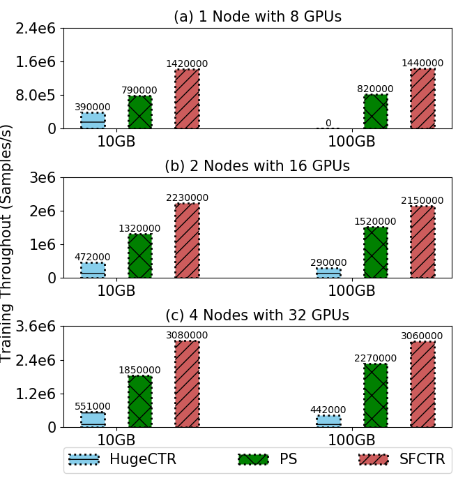
Figure 7. The training throughout comparison of SFCTR, HugeCTR and PS.

To compare the scalability of SFCTR with HugeCTR and PS, we conduct the experiments under three cases with different computational resources: (1) 1 node with 8 GPUs; (2) 2 nodes with 16 GPUs; (3) 4 nodes with 32 GPUs. Figure 7 shows the training throughouts of the three compared systems with 10 GB and 100 GB embedding tables (in fact 30 GB and 300 GB parameters, respectively), in the three mentioned cases. Noted that HugeCTR is not applicable with 300 GB embedding parameters in 8 GPUs because the HBM of GPU(s) cannot afford the corresponding embedding parameters. We summarize the observations from Figure 7 as follows.

• Equipped with VSI operation, MixCache mechanism and 3-stage pipeline, SFCTR achieves the highest training throughout under all the settings. The size of embedding parameters does not impact on the thoughout of SFCTR much. When 4 nodes with 32 GPUs are available, the acceleration of SFCTR compared to PS (HugeCTR) is 1.6X (5.6X) and 1.3X (6.9X) with 10 GB and 100 GB embedding table, respectively.

• The size of a model that can be trained by HugeCTR is limited by the number of cards available. With eight GPUs, HugeCTR cannot even train a model with 100 GB embedding table (300 GB embedding parameters), because HugeCTR only utilizes the HBM of GPUs to store the embeddings.

• As VSI operation reduces the amount of communication data between GPU-GPU, SFCTR is more efficient than HugeCTR. SFCTR is also superior to PS, which thanks to eliminating the latency between Host-GPU by MixCache.

7.3. The Study of VSI (RQ2)

Figure 8 presents the amount of communication data reduced and the training time saved with the utilization of VSI. Recall that VSI operation sets a global identifier to each feature and eliminates duplicate features in the global batch, which benefits from the following two aspects: (1) it avoids repeatedly transferring duplicate features from Host to cache buffer in GPUs, which reduces the amount of parameters/gradients transfer between Host-GPUs; (2) it helps construct a uniform representation of working embedding parameters which introduces a more efficient GPU-GPU communication scheme. As Figure 8 shows, when 4 nodes with 32 GPUs are available, the amount of parameters/gradients transfer between Host-GPU and the communication time between GPU-GPU reduces 94% and 88%, respectively, with VSI operation.

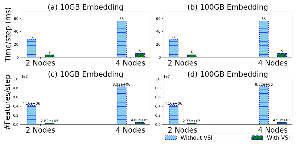
Figure 8. The comparison of data transfer between using VSI and not using VSI.

7.4. The Study of MixCache (RQ3)

7.4.1. The cache mechanism

To study the efficiency improvement brought by MixCache, we introduce another two strategies: Host and Prefetch. Host indicates all the embedding parameters are maintained in host memory without pre-fetching parameters in the next batch. Prefetch means prefetch working embedding parameters of next batch before the worker conducts training of current batch, without any guarantee on the consistence of parameters. Cache is the strategy that utilizes the proposed MixCache.

Figure 9 and Figure 10 present the training efficiency and training curve of the above mentioned strategies. From these figures, we have the following observations:

• As presented in Figure 9, to handle both 10 GB and 100 GB embedding tables, Prefetch strategy is more efficient than Host strategy because Prefetch overlaps fetching embedding parameters of the next batch with training the current batch to reduce the overall latency. Moreover, Cache strategy is the most efficient strategy, because the amount of transferring data in Cache strategy is smaller than that in Prefetch, which will be analyzed in Section 7.4.2.

• Compared with Host and Cache, the training curve of Prefetch in Figure 10 indicates slower convergence, since such simple strategy to prefetch the embedding parameters of the next batch is not able to guarantee the consistency of parameters. Such consistency is promised in both Host and Cache strategies while the Cache strategy implements it in a more efficient way.

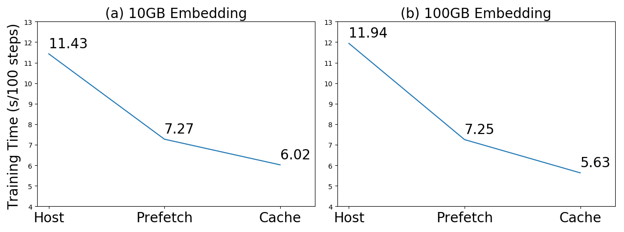
Figure 9. Training time comparison between Host, Prefetch and Cache.

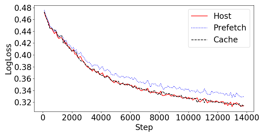
Figure 10. The training curves of Host, Prefetch and Cache strategies.

7.4.2. The parameter swapping in MixCache

To study the impact of the cache size in MixCache, we analyze the ratio of data that need to be transferred between GPU-Host in the current batch, when the cache size is varying in the range of 2 GB, 0.5 GB and 0.25 GB. The results are presented in Figure 11, where the upper (bottom) half displays the ratio of data transfer from Host to GPU (from GPU to Host) in the different training step. In detail, the red solid, blue dotted, black dashed lines represent results of 2 GB, 0.5 GB and 0.25 GB, respectively. The following observations can be concluded:

• A cache with larger cache size makes data transfer from GPU to Host starting later, because a larger cache is able to maintain more embedding parameters. Specifically, a 2 GB-size cache is able to delay the data transfer from GPU to Host after more than 1000 training steps.

• The ratio of data transfer in each step is smaller if cache size is larger. This is because the larger cache is able to maintain more embedding parameters of high-frequency features. In particular, the average ratio of data transfer between GPU-Host is around 12%, 27% and 29%, when the cache size is 2 GB, 0.5 GB and 0.25 GB, respectively.

Moreover, the analysis of parameter swapping in MixCache also explains why the amount of transferring data in Cache strategy is smaller than that in Prefetch (as in Section 7.4.1).

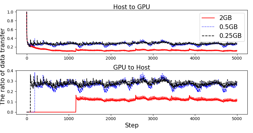
Figure 11. The ratio of data transfer between GPU and Host according to different cache sizes.

7.5. 3-Stage Pipeline (RQ4)

In this section, we investigate how effective our proposed 3-stage pipeline is in terms of training time saved. In Figure 12, the upper and bottom half present the training time of 100 million samples with 10 GB and 100 GB embedding table, respectively. There are four groups of histograms, namely the training time of single node, 2 nodes, 3 nodes and 4 nodes. Each group contains the training time of different stages.

We can observe that 3-stage pipeline is able to maximize the utilization of GPU worker. As the training time in “GPU-Worker” is the largest in all the three stages, such that GPUs can keep computing without interrupting if the other stages can be scheduled reasonably by our pipeline. As a result, our proposed 3-stage pipeline saves the training time significantly.

For example, when we use single node equipped with 3-stage pipeline to train the model with 100 GB embedding, such three stages can be scheduled reasonably and the overall training time is 75 seconds, which is the largest training time of the three stages. However, when we use single node without 3-stage pipeline, the three stages are executed sequentially and the training time of SFCTR is the summation of individual training time taken in the three stages and is around 150 seconds.

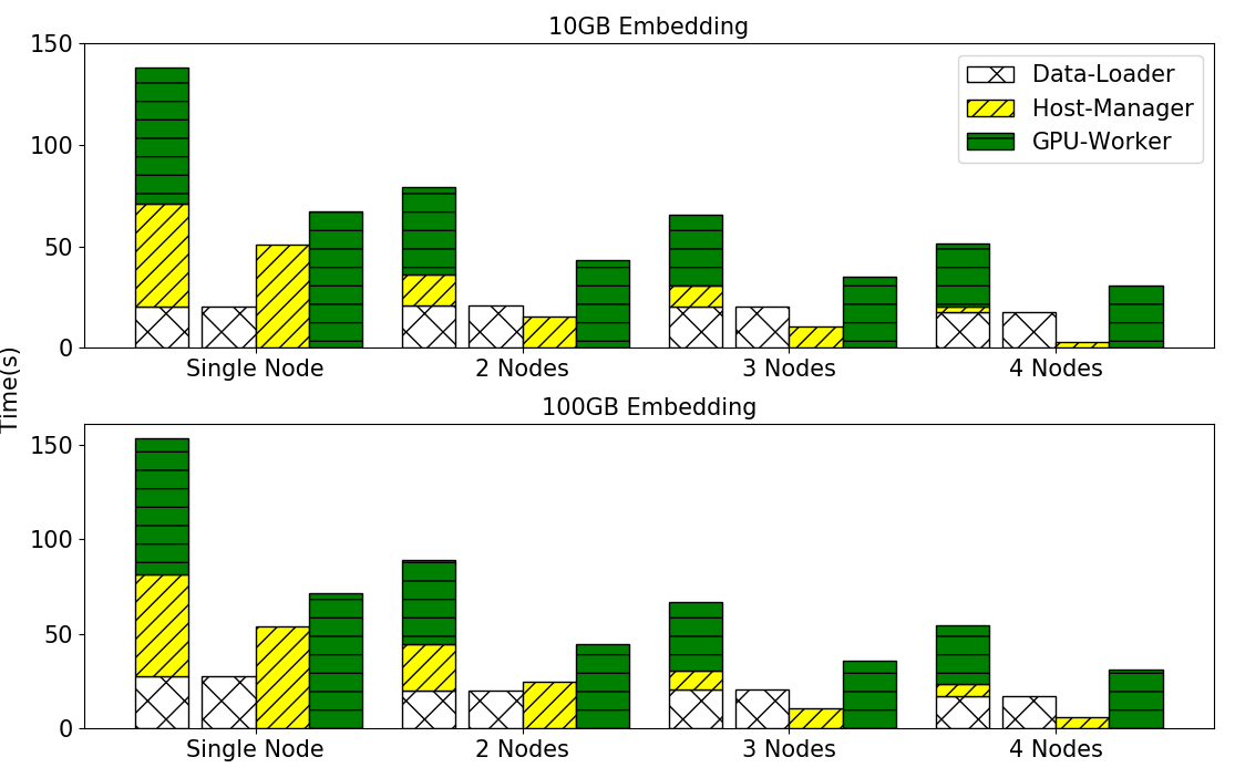
Figure 12. The training time in different stages of SFCTR.

8. Conclusion

In this paper, we propose SFCTR, a MixCache-based distributed training system for CTR models with huge embedding table. SFCTR, which consists of Data-Loader, Host-Manager and GPU-Worker, overcomes the limitations of state-of-the-art distributed training systems for CTR prediction and achieves better efficiency. Firstly, SFCTR utilizes Virtual Sparse Id operation to reduce the amount of parameters/gradients transfer between Host-GPU and GPU-GPU. Secondly, SFCTR adopts MixCache mechanism to eliminate the latency of parameters/gradients transfer between Host-GPU. Thirdly, SFCTR uses a 3-stage pipeline that overlaps Data-Loader, Host-Manager and GPU-Worker. We conduct extensive experiments and ablation studies to demonstrate the superiority of SFCTR.

There are two interesting directions for future work. One is to improve the communication efficiency (such as All2All), which will further accelerate SFCTR. The other is to investigate the fast optimization method to speed up the convergence of deep CTR model with huge embedding table.

References

- (1)
- Abadi et al. (2016) Martín Abadi, Paul Barham, Jianmin Chen, Zhifeng Chen, Andy Davis, Jeffrey Dean, Matthieu Devin, Sanjay Ghemawat, Geoffrey Irving, Michael Isard, et al. 2016. Tensorflow: A system for large-scale machine learning. In 12th USENIX Symposium on Operating Systems Design and Implementation (OSDI 16). 265–283.
- Brown et al. (2020) Tom B. Brown, Benjamin Mann, Nick Ryder, Melanie Subbiah, Jared Kaplan, Prafulla Dhariwal, Arvind Neelakantan, Pranav Shyam, Girish Sastry, Amanda Askell, Sandhini Agarwal, Ariel Herbert-Voss, Gretchen Krueger, Tom Henighan, Rewon Child, Aditya Ramesh, Daniel M. Ziegler, Jeffrey Wu, Clemens Winter, Christopher Hesse, Mark Chen, Eric Sigler, Mateusz Litwin, Scott Gray, Benjamin Chess, Jack Clark, Christopher Berner, Sam McCandlish, Alec Radford, Ilya Sutskever, and Dario Amodei. 2020. Language Models are Few-Shot Learners. CoRR abs/2005.14165 (2020).
- Chen et al. (2015) Tianqi Chen, Mu Li, Yutian Li, Min Lin, Naiyan Wang, Minjie Wang, Tianjun Xiao, Bing Xu, Chiyuan Zhang, and Zheng Zhang. 2015. Mxnet: A flexible and efficient machine learning library for heterogeneous distributed systems. arXiv preprint arXiv:1512.01274 (2015).
- Cheng et al. (2016) Heng-Tze Cheng, Levent Koc, Jeremiah Harmsen, Tal Shaked, Tushar Chandra, Hrishi Aradhye, Glen Anderson, Greg Corrado, Wei Chai, Mustafa Ispir, et al. 2016. Wide & deep learning for recommender systems. In Proceedings of the 1st workshop on deep learning for recommender systems. ACM, 7–10.
- Devlin et al. (2019) Jacob Devlin, Ming-Wei Chang, Kenton Lee, and Kristina Toutanova. 2019. BERT: Pre-training of Deep Bidirectional Transformers for Language Understanding. In Proceedings of the 2019 Conference of the North American Chapter of the Association for Computational Linguistics: Human Language Technologies. Association for Computational Linguistics, 4171–4186.
- Guo et al. (2017) Huifeng Guo, Ruiming Tang, Yunming Ye, Zhenguo Li, and Xiuqiang He. 2017. DeepFM: A Factorization-Machine Based Neural Network for CTR Prediction. In Proceedings of the 26th International Joint Conference on Artificial Intelligence (Melbourne, Australia). AAAI Press, 1725–1731.
- Guo et al. (2018) Huifeng Guo, Ruiming Tang, Yunming Ye, Zhenguo Li, Xiuqiang He, and Zhenhua Dong. 2018. DeepFM: An End-to-End Wide & Deep Learning Framework for CTR Prediction. CoRR abs/1804.04950 (2018). arXiv:1804.04950 http://arxiv.org/abs/1804.04950
- Guo et al. (2019) Huifeng Guo, Jinkai Yu, Qing Liu, Ruiming Tang, and Yuzhou Zhang. 2019. PAL: a position-bias aware learning framework for CTR prediction in live recommender systems. In RecSys. ACM, 452–456.
- Gupta et al. (2016) Suyog Gupta, Wei Zhang, and Fei Wang. 2016. Model Accuracy and Runtime Tradeoff in Distributed Deep Learning: A Systematic Study. In Proceedings of International Conference on Data Mining. IEEE Computer Society, 171–180.
- He et al. (2016) Kaiming He, Xiangyu Zhang, Shaoqing Ren, and Jian Sun. 2016. Deep Residual Learning for Image Recognition. In 2016 IEEE Conference on Computer Vision and Pattern Recognition, CVPR 2016, Las Vegas, NV, USA, June 27-30, 2016. IEEE Computer Society, 770–778.
- He et al. (2014) Xinran He, Junfeng Pan, Ou Jin, Tianbing Xu, Bo Liu, Tao Xu, Yanxin Shi, Antoine Atallah, Ralf Herbrich, Stuart Bowers, and Joaquin Quiñonero Candela. 2014. Practical Lessons from Predicting Clicks on Ads at Facebook. In Proceedings of the International Workshop on Data Mining for Online Advertising. ACM, 5:1–5:9.
- Heaton et al. (2016) J. B. Heaton, Nicholas G. Polson, and J. H. Witte. 2016. Deep Learning in Finance. CoRR abs/1602.06561 (2016).
- Ho et al. (2013) Qirong Ho, James Cipar, Henggang Cui, Seunghak Lee, Jin Kyu Kim, Phillip B. Gibbons, Garth A. Gibson, Gregory R. Ganger, and Eric P. Xing. 2013. More Effective Distributed ML via a Stale Synchronous Parallel Parameter Server. In Advances in Neural Information Processing Systems. 1223–1231.
- Huang et al. (2019) Tongwen Huang, Zhiqi Zhang, and Junlin Zhang. 2019. FiBiNET: combining feature importance and bilinear feature interaction for click-through rate prediction. In Proceedings of Conference on Recommender Systems. ACM, 169–177.
- Jiang et al. (2019) Biye Jiang, Chao Deng, Huimin Yi, Zelin Hu, Guorui Zhou, Yang Zheng, Sui Huang, Xinyang Guo, Dongyue Wang, Yue Song, et al. 2019. XDL: an industrial deep learning framework for high-dimensional sparse data. In Proceedings of the 1st International Workshop on Deep Learning Practice for High-Dimensional Sparse Data. 1–9.
- Joglekar et al. (2019) Manas R. Joglekar, Cong Li, Jay K. Adams, Pranav Khaitan, and Quoc V. Le. 2019. Neural Input Search for Large Scale Recommendation Models. CoRR abs/1907.04471 (2019). arXiv:1907.04471 http://arxiv.org/abs/1907.04471
- Juan et al. (2016) Yu-Chin Juan, Yong Zhuang, Wei-Sheng Chin, and Chih-Jen Lin. 2016. Field-aware Factorization Machines for CTR Prediction. In In RecSys. 43–50.
- Kim et al. (2019) Soojeong Kim, Gyeong-In Yu, Hojin Park, Sungwoo Cho, Eunji Jeong, Hyeonmin Ha, Sanha Lee, Joo Seong Jeong, and Byung-Gon Chun. 2019. Parallax: Sparsity-aware Data Parallel Training of Deep Neural Networks. In Proceedings of the Fourteenth EuroSys Conference. ACM, 43:1–43:15.
- Lerer et al. (2019) Adam Lerer, Ledell Wu, Jiajun Shen, Timothee Lacroix, Luca Wehrstedt, Abhijit Bose, and Alex Peysakhovich. 2019. PyTorch-BigGraph: A Large-scale Graph Embedding System. arXiv preprint arXiv:1903.12287 (2019).
- Li et al. (2014) Mu Li, David G. Andersen, Jun Woo Park, Alexander J. Smola, Amr Ahmed, Vanja Josifovski, James Long, Eugene J. Shekita, and Bor-Yiing Su. 2014. Scaling Distributed Machine Learning with the Parameter Server. In 11th USENIX Symposium on Operating Systems Design and Implementation, Jason Flinn and Hank Levy (Eds.). USENIX Association, 583–598.
- Lian et al. (2018) Jianxun Lian, Xiaohuan Zhou, Fuzheng Zhang, Zhongxia Chen, Xing Xie, and Guangzhong Sun. 2018. xDeepFM: Combining Explicit and Implicit Feature Interactions for Recommender Systems. In Proceedings of International Conference on Knowledge Discovery & Data Mining.
- Liu et al. (2019) Bin Liu, Ruiming Tang, Yingzhi Chen, Jinkai Yu, Huifeng Guo, and Yuzhou Zhang. 2019. Feature Generation by Convolutional Neural Network for Click-Through Rate Prediction. In The World Wide Web Conference. ACM, 1119–1129.
- Liu et al. (2020) Bin Liu, Niannan Xue, Huifeng Guo, Ruiming Tang, Stefanos Zafeiriou, Xiuqiang He, and Zhenguo Li. 2020. AutoGroup: Automatic Feature Grouping for Modelling Explicit High-Order Feature Interactions in CTR Prediction. In Proceedings of the 43rd International conference on research and development in Information Retrieval. ACM, 199–208.
- Mamidala et al. (2004) Amith R. Mamidala, Jiuxing Liu, and Dhabaleswar K. Panda. 2004. Efficient Barrier and Allreduce on Infiniband clusters using multicast and adaptive algorithms. In Proceedings of International Conference on Cluster Computing. IEEE Computer Society, 135–144.
- McMahan et al. (2013) H Brendan McMahan, Gary Holt, David Sculley, Michael Young, Dietmar Ebner, Julian Grady, Lan Nie, Todd Phillips, Eugene Davydov, Daniel Golovin, et al. 2013. Ad click prediction: a view from the trenches. In SIGKDD. ACM, 1222–1230.
- Naumov et al. (2019) Maxim Naumov, Dheevatsa Mudigere, Hao-Jun Michael Shi, Jianyu Huang, Narayanan Sundaraman, Jongsoo Park, Xiaodong Wang, Udit Gupta, Carole-Jean Wu, Alisson G. Azzolini, Dmytro Dzhulgakov, Andrey Mallevich, Ilia Cherniavskii, Yinghai Lu, Raghuraman Krishnamoorthi, Ansha Yu, Volodymyr Kondratenko, Stephanie Pereira, Xianjie Chen, Wenlin Chen, Vijay Rao, Bill Jia, Liang Xiong, and Misha Smelyanskiy. 2019. Deep Learning Recommendation Model for Personalization and Recommendation Systems. CoRR abs/1906.00091 (2019).
- Peng et al. (2019) Yanghua Peng, Yibo Zhu, Yangrui Chen, Yixin Bao, Bairen Yi, Chang Lan, Chuan Wu, and Chuanxiong Guo. 2019. A generic communication scheduler for distributed DNN training acceleration. In Proceedings of Symposium on Operating Systems Principles. ACM, 16–29.
- Qu et al. (2019) Yanru Qu, Bohui Fang, Weinan Zhang, Ruiming Tang, Minzhe Niu, Huifeng Guo, Yong Yu, and Xiuqiang He. 2019. Product-based Neural Networks for User Response Prediction over Multi-field Categorical Data. ACM Trans. Inf. Syst. 37, 1 (2019), 5:1–5:35.
- Rendle (2010) Steffen Rendle. 2010. Factorization machines. In 2010 IEEE International Conference on Data Mining. IEEE, 995–1000.
- Rong et al. (2020) Haidong Rong, Yangzihao Wang, Feihu Zhou, Junjie Zhai, Haiyang Wu, Rui Lan, Fan Li, Han Zhang, Yuekui Yang, Zhenyu Guo, and Di Wang. 2020. Distributed Equivalent Substitution Training for Large-Scale Recommender Systems. In Proceedings of the 43rd International ACM SIGIR conference on research and development in Information Retrieval. ACM, 911–920.
- Sergeev and Balso (2018) Alexander Sergeev and Mike Del Balso. 2018. Horovod: fast and easy distributed deep learning in TensorFlow. CoRR abs/1802.05799 (2018). http://arxiv.org/abs/1802.05799
- Valiant (1990) Leslie G. Valiant. 1990. A Bridging Model for Parallel Computation. Commun. ACM 33, 8 (1990), 103–111.
- Wang et al. (2017) Ruoxi Wang, Bin Fu, Gang Fu, and Mingliang Wang. 2017. Deep & cross network for ad click predictions. In Proceedings of the ADKDD’17. ACM, 12.
- Wang et al. (2020) Yichao Wang, Huifeng Guo, Ruiming Tang, Zhirong Liu, and Xiuqiang He. 2020. A Practical Incremental Method to Train Deep CTR Models. CoRR abs/2009.02147 (2020).
- Xu et al. (2020) Yishi Xu, Yingxue Zhang, Wei Guo, Huifeng Guo, Ruiming Tang, and Mark Coates. 2020. GraphSAIL: Graph Structure Aware Incremental Learning for Recommender Systems. CoRR abs/2008.13517 (2020).
- Yang et al. (2019) Yang Yang, Da-Wei Zhou, De-Chuan Zhan, Hui Xiong, and Yuan Jiang. 2019. Adaptive Deep Models for Incremental Learning: Considering Capacity Scalability and Sustainability. In Proceedings of International Conference on Knowledge Discovery & Data Mining. ACM, 74–82.
- Ying et al. (2018) Rex Ying, Ruining He, Kaifeng Chen, Pong Eksombatchai, William L. Hamilton, and Jure Leskovec. 2018. Graph Convolutional Neural Networks for Web-Scale Recommender Systems. In SIGKDD. ACM, 974–983.
- You et al. (2018) Yang You, Zhao Zhang, Cho-Jui Hsieh, James Demmel, and Kurt Keutzer. 2018. ImageNet Training in Minutes. In Proceedings of the 47th International Conference on Parallel Processing. ACM, 1:1–1:10.
- Zhang et al. (2016) Weinan Zhang, Tianming Du, and Jun Wang. 2016. Deep learning over multi-field categorical data. In European conference on information retrieval. Springer, 45–57.
- Zhao et al. (2020) Weijie Zhao, Deping Xie, Ronglai Jia, Yulei Qian, Ruiquan Ding, Mingming Sun, and Ping Li. 2020. Distributed Hierarchical GPU Parameter Server for Massive Scale Deep Learning Ads Systems. In Proceedings of Machine Learning and Systems 2020, Inderjit S. Dhillon, Dimitris S. Papailiopoulos, and Vivienne Sze (Eds.). mlsys.org.
- Zhou et al. (2018) Guorui Zhou, Xiaoqiang Zhu, Chengru Song, Ying Fan, Han Zhu, Xiao Ma, Yanghui Yan, Junqi Jin, Han Li, and Kun Gai. 2018. Deep Interest Network for Click-Through Rate Prediction. In Proceedings of the 24th ACM SIGKDD International Conference on Knowledge Discovery & Data Mining. 1059–1068.