DWUG: A large Resource of Diachronic Word Usage Graphs
in Four Languages

Abstract

Word meaning is notoriously difficult to capture, both synchronically and diachronically. In this paper, we describe the creation of the largest resource of graded contextualized, diachronic word meaning annotation in four different languages, based on 100,000 human semantic proximity judgments. We describe in detail the multi-round incremental annotation process, the choice for a clustering algorithm to group usages into senses, and possible – diachronic and synchronic – uses for this dataset.

1 Introduction

The view on word meaning and senses in computational linguistics has moved from a discrete (Weaver, 1949/1955; Navigli, 2009) to a graded (McCarthy and Navigli, 2009; Erk et al., 2009, 2013; Schlechtweg et al., 2018) perspective. However, scalable annotation strategies for this graded view yielding large-scale data for semantic evaluation have not been implemented yet. We build on two pre-existing schemata for graded contextual word meaning annotation (Erk et al., 2013) and show how they can be applied efficiently to create large-scale data in a diachronic setup.

Both procedures populate a Word Usage Graph (WUG, McCarthy et al., 2016; Schlechtweg et al., 2020) for a target word with annotator judgments. Procedure (i) requires annotators to judge usage pairs on a semantic proximity scale avoiding the a priori definition of word senses. This makes it preparation-lean and reduces experimenter influence. Procedure (ii) relies on a predefined list of senses and requires annotators to judge usage-sense pairs on the same proximity scale as in procedure (i). Both procedures avoid binary assignments of word senses to word usages, which have been shown to be inadequate in many cases (Kilgarriff, 1997; Hanks, 2000; Kilgarriff, 2007). The resulting graphs relate word usages to each other (either directly or indirectly) and thus allow for a posteriori hard- or soft-clustering, where clusters can be interpreted as senses (Schütze, 1998; McCarthy et al., 2016; Schlechtweg et al., 2020). This makes the collapsing of senses possible, while allowing for sense overlap where this seems adequate after observing the annotated data. While both procedures require more judgments than traditional discrete word sense annotation, we show how the sampling of word usages can be optimized to reduce the number of necessary judgments.

We apply the above-described annotation procedures in a multi-lingual diachronic setup to create Diachronic WUGs (DWUGs). These contain annotations of the usages of a set of target words in corpora from two time periods (Schlechtweg et al., 2020). This allows us to identify changes in the WUGs over time. The final resource contains 168 DWUGs for four different languages (English (EN), German (DE), Swedish (SV), Latin (LA)) relying on approximately 100,000 human judgments.

After describing the annotation procedure, we provide a detailed analysis of annotator disagreements and evaluate the robustness of the annotated graphs. DWUGs can be exploited in many ways:

• as large sets (thousands) of pairwise semantic proximity judgments to evaluate contextualized embeddings in multiple languages;

• the inferred change scores can be used to evaluate semantic change detection models

• as word sense disambiguation/discrimination resources with additional aspects such as variation over time;

• the graphs may be treated as research objects in their own right, providing insights on cognitive aspects of word meaning and posing practical problems such as finding robust and efficient clustering algorithms.

2 Related Work

There has been a significant shift in the view on word meaning and word senses in computational linguistics since the birth of the field. The early formulations of the Word Sense Disambiguation (WSD) task took a discrete view on word senses, assuming a fixed inventory of senses and a single best sense per word usage (Weaver, 1949/1955; Navigli, 2009). After this view was shown empirically to be inadequate (Kilgarriff, 1997; Hanks, 2000; Kilgarriff, 2007), researchers have increasingly adopted a graded view on word senses, whereby a word usage may be assigned to multiple senses and more fine-grained distinctions are allowed within senses (McCarthy and Navigli, 2009; Erk et al., 2009, 2013).

Moreover, various approaches on how senses can be qualified have been proposed, starting from manual sense descriptions (Wilks and Keenan, 1975), to representing a sense solely by clusters of word usages (Schütze, 1998) or by lexical substitutes (McCarthy and Navigli, 2009). Recently, developments on computational models of the meaning of individual word usages (Peters et al., 2018; Devlin et al., 2019) have inspired new research on graded word meaning (Armendariz et al., 2019).

For discrete word senses, large-scale annotation projects have been carried out, e.g. SemCor and OntoNotes (Langone et al., 2004; Hovy et al., 2006). An advantage of the graded approach is that, through bypassing sense definitions, major parts of the annotation pipeline can be automated (cf. Biemann, 2013). Studies on graded word meaning, however, cover only small amounts of data (Soares da Silva, 1992; Brown, 2008; McCarthy and Navigli, 2009; Erk et al., 2009, 2013; Hätty et al., 2019).

The above-mentioned studies have paved the way to study diachronic dimensions of meaning. So far, studies that have explicitly tried to capture this dimension are rare, small-scale and mostly assume discrete word senses (Bamman and Crane, 2011; Lau et al., 2012; Cook et al., 2014; Tahmasebi and Risse, 2017; Schlechtweg et al., 2017; Perrone et al., 2019; Basile et al., 2020; Perrone et al., 2021). The most recent approaches take a graded view (Giulianelli et al., 2020; Rodina and Kutuzov, 2020) building on the DURel framework (Schlechtweg et al., 2018), but result in little annotated data. We release the largest known resource of diachronic contextualized graded word meaning. Our resource is related to discrete word sense annotation resources such as SemCor or OntoNotes in providing groups of word usages with the same/similar senses. However, they differ from those resources in the way in which senses are obtained, i.e., inferred on the pairwise annotated data and the graded nature of usage-usage and usage-sense comparisons. In this, our resources are strongly related to USim and WSim-2 (Erk et al., 2013), but differ from these by the additional diachronic dimension, the size of the graphs and the principled and robust approach to clustering.

	$C_{1}$	$C_{2}$
English	CCOHA 1810–1860	CCOHA 1960–2010
German	DTA 1800–1899	BZ+ND 1946–1990
Swedish	Kubhist 1790–1830	Kubhist 1895–1903
Latin	LatinISE -200–0	LatinISE 0–2000

Table 1: Time-defined subcorpora for each language from which annotation data was sampled.

3 Data

The data for annotation was sampled from two time-specific historical subcorpora for each language as summarized in Table 1. For English, we used the Clean Corpus of Historical American English (CCOHA, Davies, 2012; Alatrash et al., 2020), which spans 1810s–2000s. For German, we used the DTA corpus Deutsches Textarchiv (2017) and a combination of the BZ and ND corpora Berliner Zeitung (2018); Neues Deutschland (2018). DTA contains texts from different genres spanning the 16th–20th centuries. BZ and ND are newspaper corpora jointly spanning 1945–1993. For Latin, we used the LatinISE corpus McGillivray and Kilgarriff (2013) spanning from the 2nd century B.C. to the 21st century A.D. For Swedish, we used the Kubhist corpus Språkbanken (downloaded in 2019), a newspaper corpus containing texts from 18th–20th century. The corpora are automatically lemmatised and POS-tagged. CCOHA and DTA are spelling-normalized. BZ, ND and Kubhist contain frequent OCR errors Adesam et al. (2019); Hengchen et al. (2021).

For each language half of the target words ($\approx$ 20) were chosen as words for which a change between $C_{1}$ and $C_{2}$ was described in etymological or historical dictionaries OED (2009); Paul (2002); Clackson (2011); Svenska Akademien (2009). The other half was determined by sampling a control counterpart with the same POS and comparable frequency development between $C_{1}$ and $C_{2}$ as the corresponding target word. (For details refer to Schlechtweg et al. (2020).)

$\Bigg{\uparrow}$	Identity
	Context Variance
	Polysemy
	Homonymy

$\Bigg{\uparrow}$	4: Identical
	3: Closely Related
	2: Distantly Related
	1: Unrelated

Table 2: Blank (1997)’s continuum of semantic proximity (left) and the DURel relatedness scale derived from it (right).

Figure 1: Usage-usage graphs of English plane (left), German ausspannen (middle) and Swedish ledning (right). Nodes represent usages of the respective target word. Edge weights represent the median of relatedness judgments between usages (black/gray lines for high/low edge weights, i.e., weights $\geq$ 2.5/weights $<$ 2.5).

4 Procedure (i): Usage-Usage Graphs

We first describe the procedure devised to annotate EN, DE and SV data and later describe the procedure for LA in Sec. 5. A usage-usage graph (UUG) $\mathbf{G=(U,E,W)}$ is a weighted, undirected graph, where nodes $u\in U$ represent word usages and weights $w\in W$ represent the semantic proximity of a pair of usages (an edge) $(u_{1},u_{2})\in E$ (McCarthy et al., 2016; Schlechtweg et al., 2020). In practice, semantic proximity can be measured by human annotator judgments on a scale of relatedness (Brown, 2008; Schlechtweg et al., 2018) or similarity (Erk et al., 2013). The annotation procedure starts from a non-annotated sample of word usages and aims to populate a UUG for each target word in several rounds of annotation with human judgments of semantic relatedness. Annotators were asked to judge the semantic relatedness of pairs of word usages using the scale in Table 2. (4) and (4) show two example usages of the noun plane. Von Hassel replied that he had such faith in the plane that he had no hesitation about allowing his only son to become a Starfighter pilot. This point, where the rays pass through the perspective plane, is called the seat of their representation. Figure 1 shows three UUGs resulting from our annotation.

4.1 Annotators

We started out with four annotators per language. Following high annotation loads and dropouts, additional annotators were hired, resulting in 9/8/5 total annotators for EN/DE/SV, respectively. All annotators were native speakers and current or former university students. The number of annotators with a background in historical linguistics was two for DE and one for EN and SV.

4.2 Usage sampling

We refer to an occurrence of a word $w$ in a sentence by ‘usage of $w$’. For each target word, 100 usages were randomly sampled from each of $C_{1}$ and $C_{2}$ (Table 1). Each usage contained the target word in its lemma form and a minimum of ten tokens, yielding a total of 200 usages per target word. If a target word had less than 100 usages, the full sample was annotated. The usage samples were subsequently mixed into a joint set $U$ per target word. The set of usages $U$ were annotated by presenting usage pairs to annotators in randomized order, hence, the annotators did not know from which time period each usage stemmed.

4.3 Edge sampling

Annotating the full usage graph is not feasible even for a small set of $n$ usages as this implies annotating $n*(n-1)/2$ edges. Hence, the main challenge with this annotation approach was to annotate as few edges as possible, while keeping the information needed to infer a meaningful clustering on the graph. This was achieved by annotating the data in several rounds. After each round, the UUG of a target word was updated with the new annotations and a new clustering was obtained. Based on this clustering, the edges for the next round were sampled through heuristics similar to Biemann (2013). The annotation load was randomly distributed making sure that roughly half of the usage pairs were annotated by more than one annotator.

The first round aimed to obtain a small high-quality reference set of clusters. This was achieved through the sampling of 10% of the usages from $U$ and 30% of the edges by a random walk through the sample graph (exploration), which guaranteed that all nodes are connected by some path. Hence, the first clustering was obtained on a small but richly-connected subgraph ensuring that not too many clusters were inferred, as this would lead to a strong increase in annotation instances in the subsequent rounds. In the second round, the reference clusters from the first round served as a comparison for those usages which were not assigned to a multi-cluster yet (combination). In all subsequent rounds, both a combination step and an exploration step were employed. The combination step combined each single usage $u_{1}$ which is not yet member of a multi-cluster with a random usage $u_{2}$ from each of the multi-clusters to which $u_{1}$ had not yet been compared. The exploration step consisted of a random walk on 30% of the edges from the non-assignable usages, i.e., usages which had already been compared to each of the multi-clusters but were not assigned to any of these by the clustering algorithm. This procedure slowly populated the graph while minimizing the annotation of redundant information. We aimed to stop the procedure when each cluster had been compared to each other cluster. The sample sizes for the random walk were tuned and validated in a simulation study (Schlechtweg et al., 2020).

$G$

$G_{1}$

$G_{2}$

Figure 2: Usage-usage graph of Swedish ledning (left), subgraph for first time period $C_{1}$ (middle) and second time period $C_{2}$ (right).

• The above procedure was combined with further heuristics added after round 1 to increase the quality of the annotation: (i) sampling a low number of randomly chosen edges and edges between already confirmed multi-clusters for further annotation to corroborate the inferred structure; (ii) detecting relevant disagreements between annotators, i.e., judgments with a difference of $\geq 2$ on the scale or edges with a median $\approx 2.5$, and redistributing the corresponding edges to another randomly chosen annotator from the ones who did not annotate the respective edge yet to resolve the disagreements; and (iii) detecting clustering conflicts, i.e., positive edges between clusters and negative edges within clusters (see below) and sampling a new edge for each node connected by a conflicting edge. This added more information in regions of the graph where finding a good clustering was hard. Furthermore, after each round, nodes from the graph whose 0-judgments (undecidable) made up more than half of their total judgments were removed, and in a few cases, whole words were removed if they had a high number of ‘0’ judgments or needed a high number of further edges to be annotated. The annotation was stopped after four rounds for time constraints.

(An example of our annotation pipeline can be found in Appendix A.)

4.4 Clustering

Tasks such as SemEval-2020 Task 1 require to derive a hard-clustering from the graphs. The UUGs obtained from the annotation were weighted, undirected, sparsely observed and noisy. This called for a robust clustering algorithm. For this, a variation of correlation clustering (Bansal et al., 2004; Schlechtweg et al., 2020) was employed minimizing the sum of cluster disagreements, i.e., the sum of negative edge weights within clusters plus the sum of positive edge weights across clusters. To see this, consider Blank (1997)’s continuum of semantic proximity and the DURel relatedness scale derived from it, as illustrated in Table 2. In line with Blank, usage pairs with judgments of 3 and 4 are expected to belong to the same sense, while judgments of 1 and 2 belong to different senses. Consequently, the weight $W(e)$ of all edges $e\in E$ in a UUG $\mathbf{G=(U,E,W)}$ are shifted to $W^{\prime}(e)=W(e)-2.5$ (e.g. a weight of $4$ becomes $1.5$). Those edges $e$ with a weight $W^{\prime}(e)\geq 0$ are referred to as positive edges $P_{E}$, while edges with weights $W^{\prime}(e)<0$ are called negative edges $N_{E}$. Let further $C$ be some clustering on $U$, $\phi_{E,C}$ be the set of positive edges across any of the clusters in clustering $C$ and $\psi_{E,C}$ the set of negative edges within any of the clusters. We then search for a clustering $C$ that minimizes $L(C)$:

$$L(C)=\sum_{e\in\phi_{E,C}}W^{\prime}(e)+\sum_{e\in\psi_{E,C}}|W^{\prime}(e)|~{}~{}.$$ (1)

That is, the sum of positive edge weights between clusters and (absolute) negative edge weights within clusters is minimized. Minimizing $L$ is a discrete optimization problem which is NP-hard Bansal et al. (2004), which is eased by the relatively low number of nodes ($\leq 200$). Hence, the global optimum can be approximated sufficiently with a standard optimization algorithm such as Simulated Annealing Pincus (1970): an algorithm that has shown superior performance in a previous simulation study by Schlechtweg et al. (2020). Since we do not have strong efficiency constraints, we follow the same procedure. In order to reduce the search space, we iterate over different values for the maximum number of clusters. We also iterate over randomly, as well as heuristically, chosen initial clustering states. This way of clustering usage graphs has several advantages: (i) It finds the optimal number of clusters on its own. (ii) It easily handles missing information (non-observed edges). (iii) It is robust to errors by using the global information on the graph. That is, one wrong judgment can be outweighed by correct ones. (iv) It directly optimizes an intuitive quality criterion on usage graphs. Many other clustering algorithms such as Chinese Whispers Biemann (2006) make local decisions, so that the final solution is not guaranteed to optimize a global criterion such as $L$. (v) By weighing each edge with its (shifted) weight, $L$ respects the gradedness of word meaning. That is, edges with $|W^{\prime}(e)|\approx 0$ have less influence on $L$ than edges with $|W^{\prime}(e)|\approx 1.5$. The clustered graphs are provided with the published data. Figure 2 ($G$) shows the annotated and clustered UUG for SV ledning. Nodes represent usages of the target word (isolates removed). Edges represent the median of relatedness judgments between usages. Colors make clusters (senses) inferred on the full graph $G$. $G_{1}$ (left) and $G_{2}$ (right) represent the time-specific subgraphs resulting from removing the respective nodes and their edges for each time period ($C_{1}$, $C_{2}$) from the full graph.

Figure 3: Usage-sense graphs of Latin pontifex (left), potestas (middle) and sacramentum (right). Nodes in blue/red represent usages/senses respectively.

5 Procedure (ii): Usage-Sense Graphs

In this section, we describe the procedure devised to annotate the Latin data. This procedure is different from the other languages, as in a trial annotation task the annotators reported difficulties to judge usage-usage pairs. In consideration of this, usage-sense graphs were employed. Since we do not have access to native speakers of Latin, eight annotators with a high-level knowledge of Latin were recruited, ranging from undergraduate students to PhD students, post-doctoral researchers, and more senior researchers.

5.1 Usage-sense graphs

A usage-sense graph (USG) $\mathbf{G=(V,E,W)}$ is a weighted, undirected graph, whose nodes $v\in V$ represent either word usages or sense descriptions and weights $w\in W$ represent the semantic proximity of a usage-sense pair $(u_{1},s_{1})\in E$. We denote the set of word usages as $U$ and the set of word sense descriptions as $S$, where $V=U\cup S$. Following Erk et al. (2013), semantic proximity can be measured by human annotator judgments on a similar scale as for USGs. Hence, we started from a non-annotated sample of usage-sense pairs and populated a USG for each target word with human judgments of semantic relatedness. Annotators were asked to judge the semantic relatedness of usage-sense pairs using the scale as for the other languages. (5.1) contains an example of a usage-sense pair for sacramentum, displaying the older sense “a civil suit or process” Usage: Cum Arretinae mulieris libertatem defenderem et Cotta xviris religionem iniecisset non posse nostrum sacramentum iustum iudicari, […
‘When I was defending the liberty of a woman of Arretium, and when Cotta had suggested a scruple to the decemvirs that our action was not a regular one, […] ’
Sense: “a cause, a civil suit or process” Figure 3 shows three USGs resulting from our annotation. The first word, pontifex, originally meant “a member of the college of priests having supreme control in matters of public religion in Rome”, and with Christianity it acquired the sense of “bishop”. The three senses presented to the annotators were “priest, high priest”, “Roman high-priest, a pontiff, pontifex”, and “bishop”. The first two correspond to the two red nodes in the bottom left corner of the first plot in Figure 3, and the last one corresponds to the top right red node. The plot of the second word, potestas shows the complex and highly related set of its senses, which can be summarised as: “Power of doing any thing”; “Political power”; “Magisterial power”; “Meaning of a word” (the isolated sense on the far right of the plot); “Force, efficacy”; “Angelic powers”. The last plot refers to sacramentum and shows how the two senses “military oath of allegiance” and “oath” are close together on the top left of the plot, while the legal sense “a civil suit or process” is separated from the others in the top right corner and the Christian sense of “sacrament” is at the bottom right corner.

$G$

$G_{1}$

$G_{2}$

Figure 4: Usage-sense graph of Latin sacramentum (left), subgraph for first time period $C_{1}$ (middle) and second time period $C_{2}$ (right).

5.2 Usage and sense sampling

For each target word, 30 usages from each of $C_{1}$ and $C_{2}$ containing $\geq 2$ tokens were randomly sampled, yielding a total of 60 usages per target word. The sense definitions were taken from the Latin portion of the Logeion online dictionary. Due to the challenge of finding qualified annotators, each word was assigned to one annotator, apart from virtus, which was annotated by four annotators and used for inter-annotator agreement (Table 3). The annotators could add comments to their annotations. The senses and usages were presented in randomized order to the annotators.

5.3 Edge sampling

Procedure (ii) has an upper bound on the total number of annotated usage-sense pairs of $n\times k$ with $k$ senses for $n$ usages. The number of senses ranged between 2 and 7 with a usage sample size of $60$ which yielded a good number of annotation instances. Hence, no further optimization of the edge sampling procedure was carried out. Note though that a similar optimization as for procedure (i) would be possible by annotating the data incrementally or by randomly subsampling edges.

5.4 Clustering

From the annotation, USGs where each usage is connected to each sense by one edge (see Figure 3) were obtained. Therefore there is a first-order path between each usage-sense pair and a second-order path between each usage-usage pair. Similarly to UUGs, we wanted to assign usages and senses into the same cluster if they received high judgments (3, 4) and into different clusters if they received low judgments (1, 2). We used the same clustering algorithm as for UUGs, defined in Section 4.4. In this way, usages end up in the same cluster if they have high judgments with the same senses. If there are contradictory judgments (e.g. a usage has high judgments with several senses), the clustering uses the global information to decide on the cluster assignment by choosing the one with the lowest loss. This can also lead to the collapsing of two sense descriptions into one cluster, e.g. for Latin sacramentum in Figure 4.

LGS	$\mathbf{n}$	N/V/A	$\mathbf{|U|}$	AN	JUD	AV	SPR	KRI	LOSS
EN	40	36/4/0	189	9	29k	2	.69	.61	.16
DE	48	32/14/2	178	8	37k	2	.59	.53	.12
SV	40	31/6/3	168	5	20k	2	.57	.56	.08
LA	40	27/5/8	59	1	9k	1	.64	.62	.16

Table 3: Overview target words. LGS = language, $n$ = no. of target words, N/V/A = no. of nouns/verbs/adjectives, $|U|$ = avg. no. usages per word, AN = no. of annotators, JUD = total no. of judged usage pairs, AV = avg. no. of judgments per usage pair, SPR = weighted mean of pairwise Spearman in round 1, KRI = Krippendorff’s alpha in round 1, LOSS = avg. of normalized clustering loss * 10.

6 Resource

A summary of the annotation outcome for each language can be found in Table 3. The final resource contains 40 words for EN/SV/LA, and 48 words for DE. We report two annotation agreement measures: mean pairwise Spearman correlations (Bolboaca and Jäntschi, 2006) between annotator judgments and Krippendorff’s alpha Krippendorff (2004) for judgments’ consensus, both reaching comparable scores to previous studies (Erk et al., 2013; Schlechtweg et al., 2018; Rodina and Kutuzov, 2020). The clustering loss is the value of $L$ (Definition 1) divided by the maximum possible loss on the respective graph. It gives a measure of how well the graphs could be partitioned into clusters by the $L$ criterion. In total, roughly 100,000 judgments were made by annotators. For EN/DE/SV $\approx$50% of the usage pairs were annotated by more than one annotator, while for LA each target word but one was annotated by one annotator.

Figure 5 shows the frequencies of annotator judgments over the DURel scale by language. On the UUGs (EN/DE/SV) judgment ‘4’ is most frequent followed either by judgment ‘2’ (EN/DE) or ‘1’ (SV). Least frequent are judgments of ‘0’ (‘Cannot decide’). Swedish has a considerably higher number of ‘0’ judgments, presumably because of frequent OCR errors. On the USGs (LA) judgments of ‘1’ are clearly most frequent, followed by ‘4’. This is because each usage is judged against each sense description which can often be unrelated. It can be seen that annotators make frequent use of the intermediate levels of the scale (‘2’, ‘3’) and thus assign graded distinctions of word meaning.

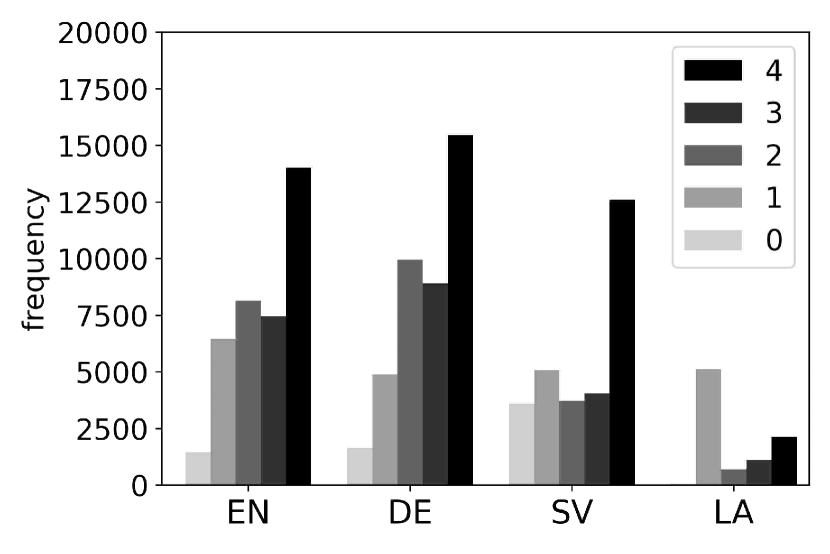
Figure 5: Judgment frequency per language.

7 Analysis

7.1 Annotator disagreements

Roughly half of all edges were annotated by only one annotator. In order to estimate the reliability of these annotations we report disagreement frequencies on all edges with two judgments as displayed in Figure 6. Annotator pairs agree on 61–69% of these edges across languages, while they disagree by one point on the scale on 27–34%. Stronger disagreements are very rare with less than 5%.

We further analyze annotator disagreements on a subset of words from the DWUG DE data set covering different POS (abbauen (VB), abgebrüht (ADJ), Knotenpunkt (NN), Manschette (NN), zersetzen (VB)); we extract edges where at least one annotator pair diverges by at least two points on the DURel scale in Table 2 (e.g. 1/3). We identify 5 sources of disagreement:

• ambiguity

• meaning unfamiliarity

• misleading context

• unclear meaning abstraction level

• different intuitions on semantic proximity

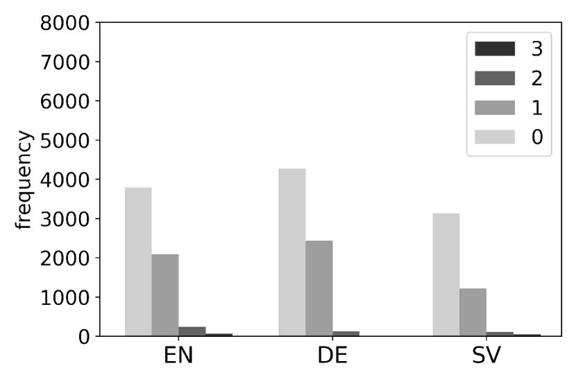
Figure 6: Disagreement frequency on edges with two annotations. Numbers in legend correspond to disagreements by points on the DURel scale.

Most cases of disagreements between annotators can be traced back to ambiguity or meaning unfamiliarity with one of the usages. das war ein finsterer Herr mit dem harten Blick eines abgebrühten Schellfisches.
‘that was a sinister gentleman with the hard look of a blanched/hard-nosed haddock’ Darum hatte Calloway solche Manschetten, was?
‘That’s why Calloway had fear/cuffs/collars like that, huh?’ Vor allem Gregor Strasser war einer der braunen Halbgötter, bis er 1932 kurzerhand von Hitler abgebaut wurde.
‘Above all Gregor Strasser was one of the brown demigods until he was destroyed?/deprived? by Hitler in 1932.’ (7.1) is a case of ambiguity: abgebrüht modifies an animal which could be “blanched” in the literal sense, but could also mean “hard-nosed” as the animal is further attributed with a “hard glance”. Often ambiguity is also triggered by missing sentence context. (7.1) is a short sentence which gives little clues on the meaning of the target word. Manschetten is at least ambiguous between a “fear”, a “cuff” and a “collar” reading. In (7.1) abgebaut occurs in an archaic sense which was only observed once in our data and is likely unfamiliar to annotators. The context and its other senses suggest a meaning like “to destroy, to deprive”, but the exact meaning is unclear. Further cases include usages with misleading context where a superficial reading or certain key words suggest a specific reading, while a deeper reading suggests another, and usages where the meaning of the target word could be described on various abstraction levels. There are also a few cases where the above categories do not apply, which may be due to (genuinely) different intuitions on semantic proximity.

7.2 Robustness

To estimate if the clustering method is sensitive to spurious errors in the annotation procedure, we tested the robustness of our results to perturbations in the graphs’ weights. We replaced existing annotations with random scores (i.e., changing scores only for existing annotation pairs), created new graphs, and clustered them. We then compared the similarity between the clusters in the original graphs, which we viewed as true labels, to those of the manipulated graphs using cluster accuracy. This analysis, computed on English graphs (Figure 7), demonstrates that the cluster structure of the graphs is robust under relatively high degree of random annotations: at an error rate of 25% of the annotations, the manipulated graphs have cluster accuracy greater than 80% on average.

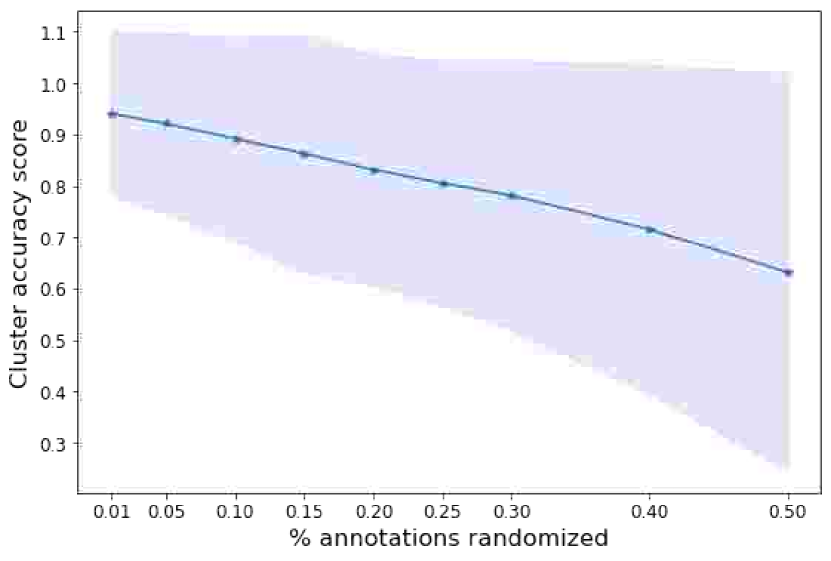
Figure 7: Mean cluster accuracies and CI (y axis) for increasing proportions of random annotations (x axis).

8 Conclusion

We described the creation of the largest existing resource of word usage graphs that capture graded, contextualized word meaning for four languages, namely English, German, Swedish and Latin. We detailed the annotation procedure, including the sampling aimed to reduce annotation effort while keeping a high density in regions where annotators have difficulty judging relatedness. The usage graphs have been clustered and we openly release clusterings, visualizations and an analysis of the clustering results. This resource has been used for the SemEval 2020 task on unsupervised lexical semantic change detection, but its possibilities are much broader and range from the use of different clustering techniques, including soft-clustering, to the use as ground truth for diachronic word sense disambiguation or temporal classification of sentences. The corpora used and some aspects of the annotation procedure were different for Latin, and this was a necessary choice due to the lack of native speakers for this language and to the nature of the texts at our disposal. Offering a resource for Latin attests to the methodological and intellectual contribution of our work and we believe in the value of working on lexical semantic change for a historical language.

Future work entails annotating additional critical edges to allow for better understanding of robustness; how much annotation is needed for different kinds of words? Knowing that some words, e.g., single-sense concrete words, require less annotation allows us to spend more effort on abstract and highly polysemous words. We will also analyze the influence of edge sparsity and ambiguity on the clustering procedure and compare its output to other annotation strategies.

Appendix A Annotation pipeline example

Figure 8 shows an example of our annotation pipeline. As the annotation proceeds through the rounds, the graph becomes more populated and the true cluster structure is found. In round 1 one multi-cluster is found. Hence, all remaining usages are compared with this cluster in round 2 by the combination step. In rounds 3 and 4 the exploration step discovers more clusters not found in the rounds before.

round 0

round 1

round 2

round 3

round 4

round 5

Figure 8: Simulated example of annotation pipeline.

References

- Adesam et al. (2019) Yvonne Adesam, Dana Dannélls, and Nina Tahmasebi. 2019. Exploring the quality of the digital historical newspaper archive KubHist. In Proceedings of the 2019 DHN conference, pages 9–17.
- Alatrash et al. (2020) Reem Alatrash, Dominik Schlechtweg, Jonas Kuhn, and Sabine Schulte im Walde. 2020. CCOHA: Clean Corpus of Historical American English. In Proceedings of the 12th Language Resources and Evaluation Conference, pages 6958–6966, Marseille, France. European Language Resources Association.
- Armendariz et al. (2019) Carlos Santos Armendariz, Matthew Purver, Matej Ulčar, Senja Pollak, Nikola Ljubešić, Marko Robnik-Šikonja, Mark Granroth-Wilding, and Kristiina Vaik. 2019. Cosimlex: A resource for evaluating graded word similarity in context. ArXiv, abs/1912.05320.
- Bamman and Crane (2011) David Bamman and Gregory Crane. 2011. Measuring historical word sense variation. In Proceedings of the 11th Annual International ACM/IEEE Joint Conference on Digital Libraries, pages 1–10, New York, NY, USA. ACM.
- Bansal et al. (2004) Nikhil Bansal, Avrim Blum, and Shuchi Chawla. 2004. Correlation clustering. Machine Learning, 56(1-3):89–113.
- Basile et al. (2020) Pierpaolo Basile, Annalina Caputo, Tommaso Caselli, Pierluigi Cassotti, and Rossella Varvara. 2020. Overview of the EVALITA 2020 Diachronic Lexical Semantics (DIACR-Ita) Task. In Proceedings of the 7th evaluation campaign of Natural Language Processing and Speech tools for Italian (EVALITA 2020), Online. CEUR.org.
- Berliner Zeitung (2018) Berliner Zeitung. Diachronic newspaper corpus published by Staatsbibliothek zu Berlin [online]. 2018.
- Biemann (2006) Chris Biemann. 2006. Chinese whispers: An efficient graph clustering algorithm and its application to natural language processing problems. In Proceedings of the First Workshop on Graph Based Methods for Natural Language Processing, TextGraphs-1, page 73–80, USA. Association for Computational Linguistics.
- Biemann (2013) Chris Biemann. 2013. Creating a system for lexical substitutions from scratch using crowdsourcing. Lang. Resour. Eval., 47(1):97–122.
- Blank (1997) Andreas Blank. 1997. Prinzipien des lexikalischen Bedeutungswandels am Beispiel der romanischen Sprachen. Niemeyer, Tübingen.
- Bolboaca and Jäntschi (2006) Sorana-Daniela Bolboaca and Lorentz Jäntschi. 2006. Pearson versus spearman, kendall’s tau correlation analysis on structure-activity relationships of biologic active compounds. Leonardo Journal of Sciences, 5(9):179–200.
- Brown (2008) Susan Windisch Brown. 2008. Choosing sense distinctions for WSD: Psycholinguistic evidence. In Proceedings of the 46th Annual Meeting of the Association for Computational Linguistics on Human Language Technologies: Short Papers, pages 249–252, Stroudsburg, PA, USA.
- Clackson (2011) James Clackson. 2011. A Companion to the Latin Language. Wiley-Blackwell.
- Cook et al. (2014) Paul Cook, Jey Han Lau, Diana McCarthy, and Timothy Baldwin. 2014. Novel word-sense identification. In 25th International Conference on Computational Linguistics, Proceedings of the Conference: Technical Papers, pages 1624–1635, Dublin, Ireland.
- Davies (2012) Mark Davies. 2012. Expanding Horizons in Historical Linguistics with the 400-Million Word Corpus of Historical American English. Corpora, 7(2):121–157.
- Deutsches Textarchiv (2017) Deutsches Textarchiv. Grundlage für ein Referenzkorpus der neuhochdeutschen Sprache. Herausgegeben von der Berlin-Brandenburgischen Akademie der Wissenschaften [online]. 2017.
- Devlin et al. (2019) Jacob Devlin, Ming-Wei Chang, Kenton Lee, and Kristina Toutanova. 2019. BERT: Pre-training of deep bidirectional transformers for language understanding. In Proceedings of the 2019 Conference of the North American Chapter of the Association for Computational Linguistics: Human Language Technologies, Volume 1 (Long and Short Papers), pages 4171–4186, Minneapolis, Minnesota. Association for Computational Linguistics.
- Erk et al. (2009) Katrin Erk, Diana McCarthy, and Nicholas Gaylord. 2009. Investigations on word senses and word usages. In Proceedings of the Joint Conference of the 47th Annual Meeting of the ACL and the 4th International Joint Conference on Natural Language Processing of the AFNLP: Volume 1, pages 10–18, Stroudsburg, PA, USA.
- Erk et al. (2013) Katrin Erk, Diana McCarthy, and Nicholas Gaylord. 2013. Measuring word meaning in context. Computational Linguistics, 39(3):511–554.
- Giulianelli et al. (2020) Mario Giulianelli, Marco Del Tredici, and Raquel Fernández. 2020. Analysing lexical semantic change with contextualised word representations. In Proceedings of the 58th Annual Meeting of the Association for Computational Linguistics, pages 3960–3973, Online. Association for Computational Linguistics.
- Hanks (2000) Patrick Hanks. 2000. Do word meanings exist? Computers and the Humanities, 34(1/2):205–215.
- Hätty et al. (2019) Anna Hätty, Dominik Schlechtweg, and Sabine Schulte im Walde. 2019. SURel: A gold standard for incorporating meaning shifts into term extraction. In Proceedings of the 8th Joint Conference on Lexical and Computational Semantics, pages 1–8, Minneapolis, MN, USA.
- Haug and Jøhndal (2008) Dag T. T. Haug and Marius L. Jøhndal. 2008. Creating a parallel treebank of the old indo-european bible translations. In Proceedings of the Second Workshop on Language Technology for Cultural Heritage Data (LaTeCH 2008), pages 27–34.
- Hayes (2019) Genevieve Hayes. 2019. mlrose: Machine Learning, Randomized Optimization and SEarch package for Python. https://github.com/gkhayes/mlrose. Accessed: May 22, 2020.
- Hengchen et al. (2021) Simon Hengchen, Ruben Ros, Jani Marjanen, and Mikko Tolonen. 2021. A data-driven approach to studying changing vocabularies in historical newspaper collections. Digital Scholarship in the Humanities.
- Hovy et al. (2006) Eduard Hovy, Mitchell Marcus, Martha Palmer, Lance Ramshaw, and Ralph Weischedel. 2006. Ontonotes: The 90% solution. In Proceedings of the Human Language Technology Conference of the NAACL, Companion Volume: Short Papers, NAACL-Short ’06, pages 57––60, USA. Association for Computational Linguistics.
- Kilgarriff (1997) Adam Kilgarriff. 1997. "I don’t believe in word senses". Computers and the Humanities, 31(2).
- Kilgarriff (2007) Adam Kilgarriff. 2007. Word Senses, chapter 2. Springer.
- Krippendorff (2004) K. Krippendorff. 2004. Content Analysis: An Introduction to Its Methodology. Content Analysis: An Introduction to Its Methodology. Sage.
- Langone et al. (2004) Helen Langone, Benjamin R. Haskell, and George A. Miller. 2004. Annotating wordnet. In Proceedings of the Workshop Frontiers in Corpus Annotation at HLT-NAACL, Boston, MA, USA.
- Lau et al. (2012) Jey Han Lau, Paul Cook, Diana McCarthy, David Newman, and Timothy Baldwin. 2012. Word sense induction for novel sense detection. In Proceedings of the 13th Conference of the European Chapter of the Association for Computational Linguistics, pages 591–601, Stroudsburg, PA, USA.
- McCarthy et al. (2016) Diana McCarthy, Marianna Apidianaki, and Katrin Erk. 2016. Word sense clustering and clusterability. Computational Linguistics, 42(2):245–275.
- McCarthy and Navigli (2009) Diana McCarthy and Roberto Navigli. 2009. The english lexical substitution task. Language Resources and Evaluation, 43(2):139–159.
- McGillivray and Kilgarriff (2013) Barbara McGillivray and Adam Kilgarriff. 2013. Tools for historical corpus research, and a corpus of Latin. In New Methods in Historical Corpus Linguistics, Tübingen. Narr.
- Navigli (2009) Roberto Navigli. 2009. Word sense disambiguation: a survey. ACM Computing Surveys, 41(2):1–69.
- Neues Deutschland (2018) Neues Deutschland. Diachronic newspaper corpus published by Staatsbibliothek zu Berlin [online]. 2018.
- OED (2009) OED. 2009. Oxford English Dictionary. Oxford University Press.
- Paul (2002) Hermann Paul. 2002. Deutsches Wörterbuch: Bedeutungsgeschichte und Aufbau unseres Wortschatzes, 10. edition. Niemeyer, Tübingen.
- Perrone et al. (2021) Valerio Perrone, Simon Hengchen, Marco Palma, Alessandro Vatri, Jim Q. Smith, and Barbara McGillivray. 2021. Lexical semantic change for Ancient Greek and Latin. In Nina Tahmasebi, Lars Borin, Adam Jatowt, Yang Xu, and Simon Hengchen, editors, Computational Approaches to Semantic Change, Language Variation, chapter 9. Language Science Press, Berlin.
- Perrone et al. (2019) Valerio Perrone, Marco Palma, Simon Hengchen, Alessandro Vatri, Jim Q. Smith, and Barbara McGillivray. 2019. GASC: Genre-aware semantic change for ancient Greek. In Proceedings of the 1st International Workshop on Computational Approaches to Historical Language Change, pages 56–66, Florence, Italy. Association for Computational Linguistics.
- Peters et al. (2018) Matthew Peters, Mark Neumann, Mohit Iyyer, Matt Gardner, Christopher Clark, Kenton Lee, and Luke Zettlemoyer. 2018. Deep contextualized word representations. In Proceedings of the 2018 Conference of the North American Chapter of the Association for Computational Linguistics: Human Language Technologies, pages 2227–2237, New Orleans, LA, USA.
- Pincus (1970) Martin Pincus. 1970. A monte carlo method for the approximate solution of certain types of constrained optimization problems. Operations Research, 18(6):1225–1228.
- Rodina and Kutuzov (2020) Julia Rodina and Andrey Kutuzov. 2020. RuSemShift: a dataset of historical lexical semantic change in Russian. In Proceedings of the 28th International Conference on Computational Linguistics (COLING 2020). Association for Computational Linguistics.
- Schlechtweg et al. (2017) Dominik Schlechtweg, Stefanie Eckmann, Enrico Santus, Sabine Schulte im Walde, and Daniel Hole. 2017. German in flux: Detecting metaphoric change via word entropy. In Proceedings of the 21st Conference on Computational Natural Language Learning, pages 354–367, Vancouver, Canada.
- Schlechtweg et al. (2020) Dominik Schlechtweg, Barbara McGillivray, Simon Hengchen, Haim Dubossarsky, and Nina Tahmasebi. 2020. SemEval-2020 Task 1: Unsupervised Lexical Semantic Change Detection. In Proceedings of the 14th International Workshop on Semantic Evaluation, Barcelona, Spain. Association for Computational Linguistics.
- Schlechtweg et al. (2018) Dominik Schlechtweg, Sabine Schulte im Walde, and Stefanie Eckmann. 2018. Diachronic Usage Relatedness (DURel): A framework for the annotation of lexical semantic change. In Proceedings of the 2018 Conference of the North American Chapter of the Association for Computational Linguistics: Human Language Technologies, pages 169–174, New Orleans, Louisiana.
- Schütze (1998) Hinrich Schütze. 1998. Automatic word sense discrimination. Computational Linguistics, 24(1):97–123.
- Soares da Silva (1992) A. Soares da Silva. 1992. Homonímia e polissemia: Análise sémica e teoria do campoléxico. In Actas do XIX Congreso Internacional de Lingüística e Filoloxía Románicas, volume 2 of Lexicoloxía e Metalexicografía, pages 257–287, La Coruña. Fundación Pedro Barrié de la Maza.
- Språkbanken (downloaded in 2019) Språkbanken. downloaded in 2019. The Kubhist Corpus, v2. Department of Swedish, University of Gothenburg.
- Svenska Akademien (2009) Svenska Akademien. 2009. Contemporary dictionary of the Swedish Academy. The changed words are extracted from a database managed by the research group that develops the Contemporary dictionary.
- Tahmasebi and Risse (2017) Nina Tahmasebi and Thomas Risse. 2017. Finding individual word sense changes and their delay in appearance. In Proceedings of the International Conference Recent Advances in Natural Language Processing, pages 741–749, Varna, Bulgaria.
- Weaver (1949/1955) Warren Weaver. 1949/1955. Translation. In William N. Locke and A. Donald Boothe, editors, Machine Translation of Languages, pages 15–23. MIT Press, Cambridge, MA. Reprinted from a memorandum written by Weaver in 1949.
- Wilks and Keenan (1975) Yorick Wilks and Edward L. Keenan. 1975. Preference Semantics, page 329–348. Cambridge University Press.