Emergence of Lie symmetries in functional architectures learned by CNNs

In this paper we study the spontaneous development of symmetries in the early layers of a Convolutional Neural Network (CNN) during learning on natural images. Our architecture is built in such a way to mimic the early stages of biological visual systems. In particular, it contains a pre-filtering step $\ell^{0}$ defined in analogy with the Lateral Geniculate Nucleus (LGN). Moreover, the first convolutional layer is equipped with lateral connections defined as a propagation driven by a learned connectivity kernel, in analogy with the horizontal connectivity of the primary visual cortex (V1). The layer $\ell^{0}$ shows a rotational symmetric pattern well approximated by a Laplacian of Gaussian (LoG), which is a well-known model of the receptive profiles of LGN cells. The convolutional filters in the first layer can be approximated by Gabor functions, in agreement with well-established models for the profiles of simple cells in V1. We study the learned lateral connectivity kernel of this layer, showing the emergence of orientation selectivity w.r.t. the learned filters. We also examine the association fields induced by the learned kernel, and show qualitative and quantitative comparisons with known group-based models of V1 horizontal connectivity. These geometric properties arise spontaneously during the training of the CNN architecture, analogously to the emergence of symmetries in visual systems thanks to brain plasticity driven by external stimuli.

1 Introduction

The geometry of the visual system has been widely studied over years, starting from the first celebrated descriptions given by D. H. Hubel and T. N. Wiesel (Hubel and Wiesel,, 1962; Hubel,, 1987) and advancing with a number of more recent geometrical models of the early stages of the visual pathway, describing the functional architectures in terms of group invariances (Hoffman,, 1989; Petitot,, 2008; Citti and Sarti,, 2006). Some works have also focused on reproducing processing mechanisms taking place in the visual system using these models – e.g. detection of perceptual units in Sarti and Citti, (2015), image completion in Sanguinetti et al., (2008).

On the other hand, relations between Convolutional Neural Networks (CNNs) and the human visual system have been proposed and studied, in order to make CNNs even more efficient in specific tasks (see e.g. Serre et al.,, 2007). For instance, in Yamins et al., (2015) and Yamins and DiCarlo, (2016) the authors were able to study several cortical layers by focusing on the encoding and decoding ability of the visual system, whereas in Girosi et al., (1995); Anselmi et al., (2014); Poggio and Anselmi, (2016) the authors studied some invariance properties of CNNs. A parallel between horizontal connectivity in the visual cortex and lateral connections in neural networks has also been proposed in some works (see e.g. Liang and Hu,, 2015; Spoerer et al.,, 2017; Sherstinsky,, 2020). Recently, other biologically-inspired modifications of the classical CNN architectures have been introduced (Montobbio et al.,, 2019; Bertoni et al.,, 2019).

In this paper, we combine the viewpoints of these strands of research by studying the emergence of geometrical symmetries in the early layers of a biologically inspired CNN architecture. We will focus on drawing a parallel between the patterns learned from natural images by specific computational blocks of the network, and the symmetries arising in the functional architecture of the Lateral Geniculate Nucleus (LGN) and the primary visual cortex (V1).

2 Group symmetries in the early visual pathway

Over the years, the functional architecture of the early visual pathway has often been modelled in terms of geometric invariances arising in its organization, e.g. in the spatial arrangement of cell tuning across retinal locations, or in the local configuration of single neuron selectivity. Certain classes of visual cells are shown to act, to a first approximation, as linear filters on an optic signal: the response of one such cell to a visual stimulus $I$, defined as a function on the retina, is given by the integral of $I$ against a function $\psi$, called the receptive profile (RP) of the neuron:

$$z:=\int I(x,y)\psi(x,y)dxdy.$$ (1)

This is the case for cells in the Lateral Geniculate Nucleus (LGN) and for simple cells in the primary visual cortex (V1) (see e.g. Petitot,, 2008; Citti and Sarti,, 2006). Both types of cells are characterized by locally supported RPs, i.e. they only react to stimuli situated in a specific retinal region. Each localized area of the retina is known to be associated with a bank of similarly tuned cells (see e.g. Hubel and Wiesel,, 1977; Sarti and Citti,, 2015), yielding an approximate invariance of their RPs under translations.

The set of RPs of cells is typically represented by a bank of linear filters $\{\psi_{p}\}_{p\in\mathcal{G}}\subseteq L^{2}(\mathbb{R}^{2})$ (for some references see e.g. Petitot,, 2008; Citti and Sarti,, 2006; Sarti et al.,, 2008). The feature space $\mathcal{G}$ is typically specified as a group of transformations of the plane $\{T_{p},\;p\in\mathcal{G}\}$ under which the whole filter bank is invariant: each profile $\psi_{p}$ can be obtained from any other profile $\psi_{q}$ through the transformation $T_{p-q}$. The group $\mathcal{G}$ often has the product form $\mathbb{R}^{2}\times\mathcal{F}$, where the parameters $(x_{0},y_{0})\in\mathbb{R}^{2}$ determine the retinal location where each RP is centered, while $f\in\mathcal{F}$ encodes the selectivity of the neurons to other local features of the image, such as orientation and scale.

2.1 Rotational symmetry in the LGN

A crucial elaboration step for human contrast perception is represented by the processing of retinal inputs via the radially symmetric families of cells present in the LGN (Hubel and Wiesel,, 1977; Hubel,, 1987). The RPs of such cells can be approximated by a Laplacian of Gaussian (LoG):

$$\psi_{LoG}(x,y)=-\frac{1}{\pi\sigma^{4}}\left[1-\frac{x^{2}+y^{2}}{2\sigma^{2}}\right]e^{-\frac{x^{2}+y^{2}}{2\sigma^{2}}},$$ (2)

where $\sigma$ denotes the standard deviation of the Gaussian function (see e.g. Petitot,, 2008).

2.2 Roto-translation symmetries in V1 and the lateral connectivity

The invariances in the functional architecture of V1 have been described through a variety of mathematical models. The sharp orientation tuning of simple cells is the starting point of most descriptions. This selectivity is not only found in the response of each neuron to feedforward inputs, but is also reflected in the horizontal connections taking place between neurons of V1. These connections show facilitatory influences for cells that are similarly oriented; moreover, the connections departing from each neuron spread anisotropically, concentrating along the axis of its preferred orientation (see e.g. Bosking et al.,, 1997).

An established model for V1 simple cells is represented by a bank of Gabor filters $\{\psi_{x_{0},y_{0},\theta,\sigma}\}_{(x_{0},y_{0},\theta,\sigma)\in\mathbb{R}^{2}\times S^{1}\times\mathbb{R}^{2}_{+}}$ built by translations $T_{(x_{0},y_{0})}$, rotations $R_{\theta}$ and dilations $D_{\sigma_{x},\sigma_{y}}$ of the filter

$$\psi_{0,0,0,1}(x,y)=Ae^{-\frac{x^{2}+y^{2}}{2}}\cos(2\pi fx+\phi),$$ (3)

where $A$ is the amplitude and $f$ is the frequency of the filter and $\phi$ is the phase which indicates if the Gabor filter is even or odd. See e.g. Daugman, (1985) and Lee, (1996).

The evolution in time $t\mapsto a(p,t)$ of the activity of the neural population at $p\in\mathbb{R}^{2}\times\mathcal{F}$ is assumed in Bressloff and Cowan, (2003) to satisfy a Wilson-Cowan equation (Wilson and Cowan,, 1972):

$$\partial_{t}a(p,t)=-\alpha\>a(p,t)\\ +\>s\left(\int K(p,p^{\prime})a(p^{\prime},t)dp^{\prime}+z(p,t)\right).$$ (4)

Here, $s$ is a nonlinear activation function; $\alpha$ is a decay rate; $z$ is the feedforward input corresponding to the response of the simple cells in presence of a visual stimulus, as in Eq. (1); and the kernel $K$ weights the strength of horizontal connections between $p$ and $p^{\prime}$. The form of this connectivity kernel has been investigated in a number of studies employing differential geometry tools. A breakthrough idea in this direction has been that of viewing the feature space as a fiber bundle with basis $\mathbb{R}^{2}$ and fiber $\mathcal{F}$. This approach first appeared in the works of Koenderink and van Doom, (1987) and Hoffman, (1989). It was then further developed by Petitot and Tondut, (1999) and Citti and Sarti, (2006). In the latter work, the model is specified as a sub-Riemannian structure on the Lie group $\mathbb{R}^{2}\times S^{1}$ by requiring the invariance under roto-translations. Other works extended this approach by inserting further variables such as scale, curvature, velocity (see e.g. Sarti et al.,, 2008; Abbasi-Sureshjani et al.,, 2018; Barbieri et al.,, 2014).

The long-range horizontal connections of V1 are believed to constitute the neural implementation of contour completion, i.e. the ability to group local edge items into extended curves. This perceptual phenomenon has been described through association fields (Field et al.,, 1993), characterizing the geometry of the mutual influences between oriented local elements. See Figure 1A from the experiment of Field, Heyes and Hess. Association fields have been characterized in Citti and Sarti, (2006) as families of integral curves of the two vector fields

$$\vec{X_{1}}=(\cos\theta,\sin\theta,0),\;\;\;\;\vec{X_{2}}=(0,0,1)$$ (5)

generating the sub-Riemannian structure on $\mathbb{R}^{2}\times S^{1}$. Figure 1B shows the 3-D constant coefficients integral curves of the vector fields (5) and Figure 1C their 2-D projection. These integral curves are the solution of the following ordinary differential equation:

$$\gamma^{\prime}(t)=X_{1}(\gamma(t))+kX_{2}(\gamma(t)).$$

The curves starting from $(0,0,0)$ can be rewritten explicitly in the following way:

$$\begin{split}x=\frac{1}{k}sin(kt),\;\;\;\;\;\;\;y=\frac{1}{k}(1-cos(kt)),\;\;\;\;\;\;\;\theta=kt.\end{split}$$ (6)

while integral curves starting from a general point $(x_{0},y_{0},\theta_{0})$ can be generated from equations (6) by translations $T_{(x_{0},y_{0})}$ and rotations $R_{\theta}$.

The probability of reaching a point $(x,y,\theta)$ starting from the origin and moving along the stochastic counterpart of these curves can be described as the fundamental solution of a second order differential operator expressed in terms of the vector fields $\vec{X_{1}}$, $\vec{X_{2}}$. This is why the fundamental solution of the sub-Riemannian heat kernel or Fokker Planck (FP) kernel have been proposed as alternative models of the cortical connectivity. This perspective based on connectivity kernels was further exploited in Montobbio et al., (2020): the model of the cortex was rephrased in terms of metric spaces, and the long range connectivity kernel directly expressed in terms of the cells RPs: in this way a strong link was established between the geometry of long range and feedforward cortical connectivity. Finally, in Sanguinetti et al., (2010) a strong relation between these models of cortical connectivity and statistics of edge co-occurrence in natural images was proved: the FP fundamental solution is indeed a good model also for the natural image statistics. In addition, starting from a connectivity kernel parameterized in terms of position and orientation, in Sanguinetti et al., (2010) they obtained the 2-D vector field represented in red in Figure 1D , whose integral curves (depicted in blue) provide an alternative model of association fields, learned from images.

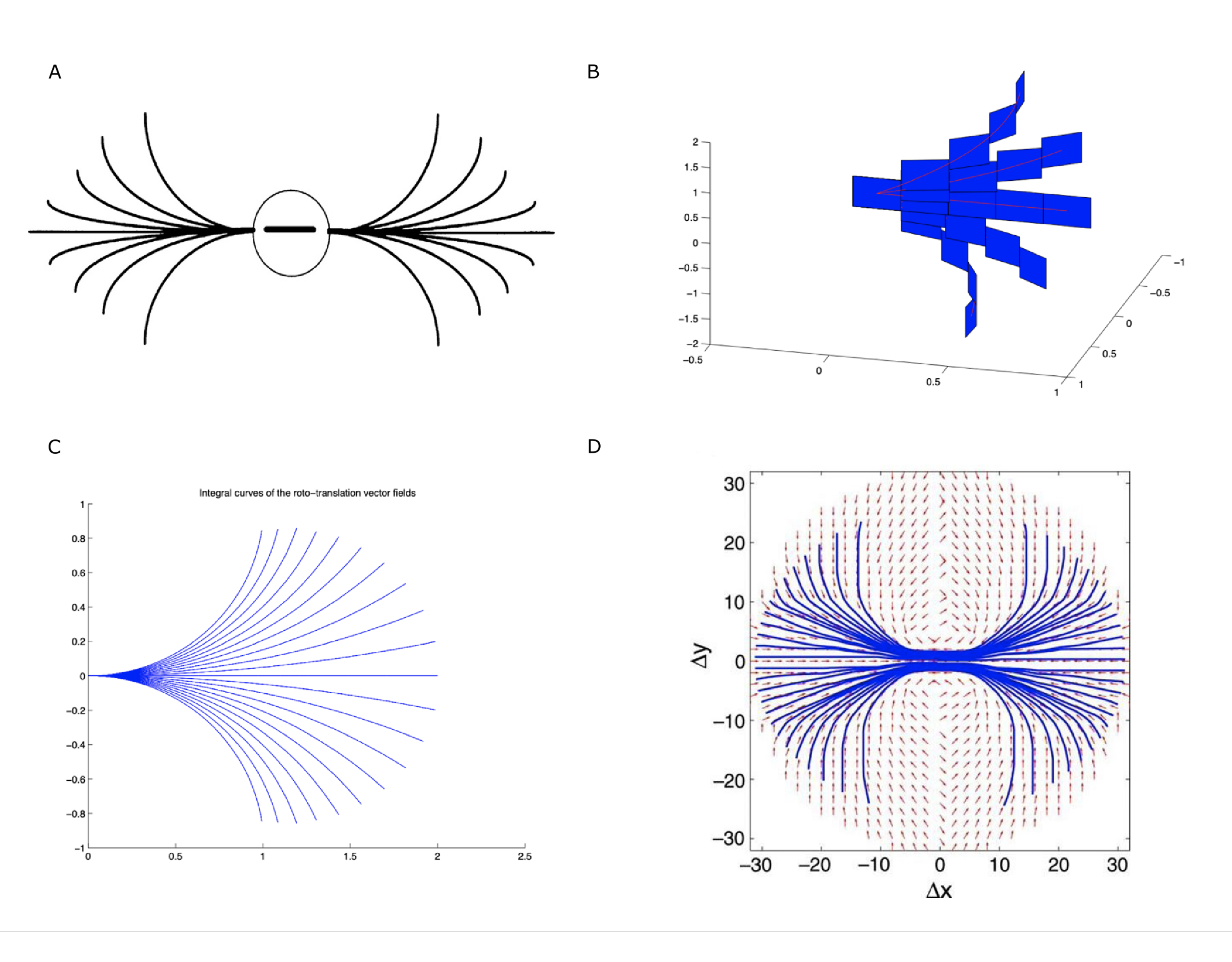
Figure 1: (A) Association fields from the experiment of Field, Hayes and Hess (Field et al.,, 1993). (B) 3D representation of the association field with contact planes of integral curves of the fields (5) with varying values of the parameter $k$, from (Citti and Sarti,, 2006). (C) Integral curves of the fields (5) with varying $k$, from (Citti and Sarti,, 2006). (D) The vector field of unitary vectors oriented with the maximal edge co-occurrence probability (red) with superimposed its integral curves (blue), from (Sanguinetti et al.,, 2010).

3 The underlying structure: a convolutional neural network architecture

In this section we introduce the network model that will constitute the fundamental structure at the basis of all subsequent analyses. The main architecture consists of a typical Convolutional Neural Network (CNN) for image classification (see e.g. Lawrence et al.,, 1997; LeCun et al.,, 1998). CNNs were originally designed in analogy with information processing in biological visual systems. In addition to the hierarchical organization typical of deep architectures, translation invariance is enforced in CNNs by local convolutional windows shifting over the spatial domain. This structure was inspired by the localized receptive profiles of neurons in the early visual areas, and by the approximate translation invariance in their tuning. We inserted two main modifications to the standard model. First, we added a pre-filtering step that mimics the behavior of the LGN cells prior to the cortical processing. Second, we equipped the first convolutional layer with lateral connections defined by a diffusion law via a learned transition kernel, in analogy with the horizontal connectivity of V1. We focused on the CIFAR-10 dataset (Krizhevsky,, 2009), since it contains natural images with a large statistics of orientations and shapes (see e.g. Ernst et al.,, 2007). We expect to find a strict similarity between the connectivity associated to this transition kernel and one observed by (Sanguinetti et al.,, 2010) since they are both learned from natural images.

3.1 LGN in a CNN

As described in Bertoni et al., (2019), since the LGN pre-processes the visual stimulus before it reaches V1, we aim to introduce a “layer 0” that mimics this behavior. To this end, a convolutional layer $\ell^{0}$ composed by a single filter $\Psi^{0}$ of size $s^{0}\times s^{0}$, a ReLU function and a batch normalization step is added at the beginning of the CNN architecture. If $\ell^{0}$ behaves similarly to the LGN, then $\Psi^{0}$ should eventually attain a rotational invariant pattern, approximating the classical Laplacian-of-Gaussian (LoG) model for the RPs of LGN cells. In such a scenario, the rotational symmetry should emerge spontaneously during the learning process induced by the statistics of natural images, in analogy with the plasticity of the brain. In Section 5 we will display the filter $\Psi^{0}$ obtained after the training of the network and test its invariance under rotations.

3.2 Horizontal connectivity of V1 in a CNN

Although the analogy with biological vision is strong, the feedforward mechanism implemented in CNNs is a simplified one, overlooking many of the processes contributing towards the interpretation of a visual scene. Our aim is to insert a simple mechanism of horizontal propagation defined by entirely learned connectivity kernels, and to analyze the invariance patterns, if any, arising as a result of learning from natural images.

Horizontal connections of convolutional type have been introduced in previous work through a recurrent formula analogous to (4), describing an evolution in time (Liang and Hu,, 2015; Spoerer et al.,, 2017). However, the lateral kernels employed in these works are very localized, so that the connectivity kernel applied at each step only captures the connections between neurons very close-by in space. Here we propose a two-step version of this model, where the output of the first layer is first mapped to the corresponding feature space through the feedforward stream, yielding an activation pattern $h^{1}=ReLU(z^{1})$, and then updated through convolution with a connectivity kernel $K^{1}$ with a wider support. The new output $\tilde{h}^{1}$ is defined by averaging between this propagated activation $K^{1}\ast h^{1}$ and the original activation $h^{1}$, so that our update rule reads:

$$\tilde{h}^{1}=\frac{1}{2}\Big{(}K^{1}\ast h^{1}\>+\>h^{1}\Big{)}.$$ (7)

The connectivity kernel $K^{1}$ is a 4-dimensional tensor parameterized by 2-D spatial coordinates $(i,j)$ and by the indices $(f,g)$ corresponding to all pairs of $\ell^{1}$ filters. For fixed $f$ and $g$, the function

$$(i,j)\mapsto K^{1}(i,j,f,g)$$ (8)

represents the strength of connectivity between the filters $\Psi_{f}$ and $\Psi_{g}$, where the spatial coordinates indicate the displacement in space between the two filters. The intuitive idea is that $K^{1}$ behaves like a “transition kernel” on the feature space of the first layer, modifying the feedforward output according to the learned connectivity between filters: the activation of a filter encourages the activation of other filters strongly connected with it. Also note that the lateral connections take the form of a linear propagation applied on top of the nonlinear activation function of the first layer. As a consequence, an even wider connectivity may be modelled by iterating the process, while still allowing to recover the resulting long-range kernel via “self-replication” through convolution against itself:

$$\frac{1}{2}\Big{(}K^{1}\ast\tilde{h}^{1}\>+\>\tilde{h}^{1}\Big{)}=\frac{1}{4}\Big{(}K^{1}\ast K^{1}\ast h^{1}\>+\>2K^{1}\ast h^{1}\>+\>h^{1}\Big{)}.$$

3.3 Description of the architecture and training parameters

In this section we shall give a detailed overview of our CNN architecture, as well as the training scheme employed.

Since we wanted a gray scale image to be the input of our neural network, we transformed the CIFAR-10 dataset into gray scale images with mean equal to 0.1307 and standard deviation equal to 0.3081. We split the entire dataset composed by 60000 images in a training set, validation set and test set (40000, 10000 and 10000 images respectively).

The architecture is composed by 11 convolutional layers, each one followed by a ReLU function and a batch normalization layer, and by 3 fully-connected layers. For simplicity we omit the ReLU function and the batch normalization layer in the architecture description. A zero padding was applied in order to keep the spatial dimensions unchanged after each convolutional layer. The architecture was defined as follows:

• LGN layer: convolutional layer $\ell^{0}$ containing a single filter $\Psi^{0}$ of size $11\times 11$;

• $\ell^{1}$ convolutional layer: 64 filters of size $7\times 7$;

• First layer lateral connections: connectivity kernel $K^{1}$ of size $13\times 13\times 64\times 64$;

• Max pooling of square size 2;

• $\ell^{2}$, $\ell^{3}$ and $\ell^{4}$ convolutional layers: $\ell^{2}$ contains 64 filters of size $5\times 5\times 64$, $\ell^{3}$ and $\ell^{4}$ contain 64 filters of size $3\times 3\times 64$;

• Max pooling of square size 2;

• $\ell^{5}$, $\ell^{6}$ and $\ell^{7}$ convolutional layers: $\ell^{5}$ and $\ell^{6}$ contain 64 filters of size $3\times 3\times 64$, whereas $\ell^{7}$ contain 128 filters of the same size;

• Max pooling of square size 2;

• $\ell^{8}$, $\ell^{9}$ and $\ell^{10}$ convolutional layers: each one contains 128 filters of size $3\times 3\times 128$;

• Max pooling of square size 2;

• 3 fully-connected layers with 1000, 200 and 10 output units respectively.

The neural network was trained using the cross entropy loss function, optimizing it via Stochastic Gradient Descent (SGD) with batch size equal to 64, where the $L^{2}$ regularization parameter $\lambda$ and the momentum were set to 0.001 and 0.9 respectively. The learning rate was 0.01 and was decreased over epochs by a factor 10 if the performance of the network on the validation set had not increased in the 10 previous epochs. The training of the neural network was performed in 2 steps: we first trained the feedforward part of the architecture, i.e. excluding the lateral connections of $\ell^{1}$; we then inserted them and trained the connectivity kernel $K^{1}$ keeping the rest of the weights fixed.

In order to increase the performance avoid overfitting, along with the weight regularization and the batch normalization layers, we applied dropout with dropping probability equal to 0.5 in the feedforward training after convolutional layer $\ell^{10}$, and 0.2 in the second training step after applying the kernel $K^{1}$. We also used an early stopping approach by terminating the optimization algorithm as soon as the performance on the validation set failed to increase for 50 consecutive epochs. The maximum number of epochs was set to 400. The network architecture and optimization procedure were coded using Pytorch (Paszke et al.,, 2017).

We want to outline that, since we are interested in the emergence of symmetries, we did not focus on reaching state-of-the-art performances on classifying the CIFAR-10 dataset. However, our architecture reaches fair performances that can be increased by adding further convolutional layers and/or increasing the number of units. We trained several CNNs varying the numbers of layers and features.

Figure 2 shows the mean performances on the test set over 20 such models with and without the lateral connectivity. As expected, increasing the number of convolutional layers and adding the lateral connection (and also the number of units) led to better performance. For the analyses described in the following, we chose the architecture that reached the best performances (79.04 % over 20 models with Horizontal connectivity), i.e. the one with 11 convolutional layers described above. However, we stress that all the architectures examined showed a comparable behavior as regards the invariance properties of the convolutional layers $\ell^{0}$ and $\ell^{1}$ and the connectivity kernel $K^{1}$. Therefore, it would be reasonable to expect a similar behavior also when further increasing the complexity of the model.

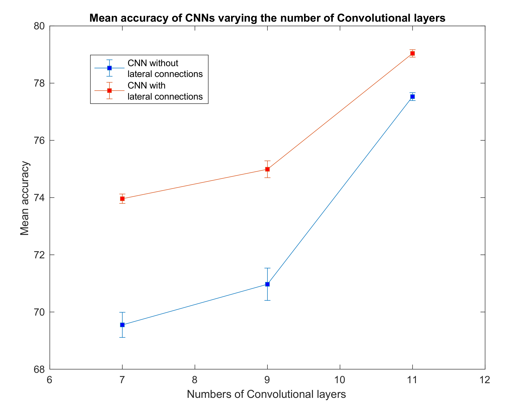
Figure 2: Mean accuracy of CNNs with varying number of convolutional layers, with and without lateral connections in the first layer. Error bars represent the standard error of the mean.

4 Emergence of rotational symmetry in the LGN layer

As described in (Bertoni et al.,, 2019) the introduction of a convolutional layer $\ell^{0}$ containing a single filter $\Psi^{0}$ mimics the role of the LGN that pre-filters the input visual stimulus before it reaches the V1 cells. The authors have shown that a rotational invariant pattern is attained by $\Psi^{0}$ for a specific architecture, suggesting that it should happen also for deeper and more complex architectures.

Figure 3A shows the filter $\Psi^{0}$ obtained after the training phase. As expected it has a radially symmetric pattern and its maximum absolute value is attained in the center. Thus it can be approximated by the classical LoG model for the RP of an LGN cell by finding the optimal value for the parameter $\sigma$ in Eq. (2). We used the built-in function optimize.curve_fit from the Python library SciPy. Figure 3B shows this approximation with $\sigma=0.184$. Applying the built-in function corrcoef from the Python library NumPy, it turns out that the two functions have a high correlation of 93.67%.

These results show that $\Psi^{0}$ spontaneously evolves into a radially symmetric pattern during the training phase, and more specifically its shape approximates the typical geometry of the RPs of LGN cells.

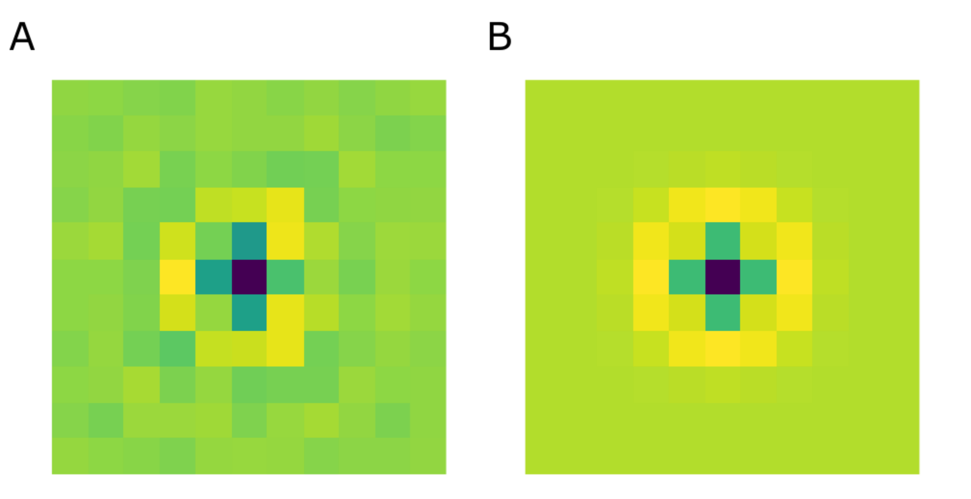
Figure 3: (A) The learned filter $\Psi^{0}$ of the current architecture. (B) Its approximation as a LoG, with optimal $\sigma=0.184$, yielding a correlation of 93.67% with the learned filter.

5 Emergence of Gabor-like filters in the first layer

As introduced in Section 2.2, the RPs of V1 simple cells can be modeled as Gabor functions by Eq. (3). Moreover, the first convolutional layer of a CNN architecture usually shows Gabor-like filters (see e.g. Serre et al.,, 2007), assuming a role analogous to V1 orientation-selective cells. In this section, we first approximate the filters of $\ell^{1}$ as a bank of Gabor filters, in order to obtain a parameterization in terms of position $(x_{0},y_{0})$ and orientation $\theta$. This will provide a suitable set of coordinates for studying the corresponding lateral kernel in the $\mathbb{R}^{2}\times S^{1}$ domain, see Section 6.

5.1 Approximation of the filters as Gabor functions

After the training phase, Gabor-like filters emerge in $\ell^{1}$ as expected (see Figure 4A). Moreover, thanks to the introduction of the pre-filtering $\ell^{0}$, our layer $\ell^{1}$ only contains filters sharply tuned for orientation, with no Gaussian-like filters. Indeed, by removing $\ell^{0}$, the two types of filters are mixed up in the same layer. See Figure 4B, showing the $\ell^{1}$ filters of a trained CNN with the same architecture, but without $\ell^{0}$.

However we can note from Figure 4A that some filters have more complex shapes that are neither Gaussian-, nor Gabor-like; indeed, since we have not introduced other geometric structures on following layers, it is reasonable to observe the emergence of more complex patterns. For the subsequent analyses, we considered the 48 filters with highest correlation with the approximating Gabor functions.

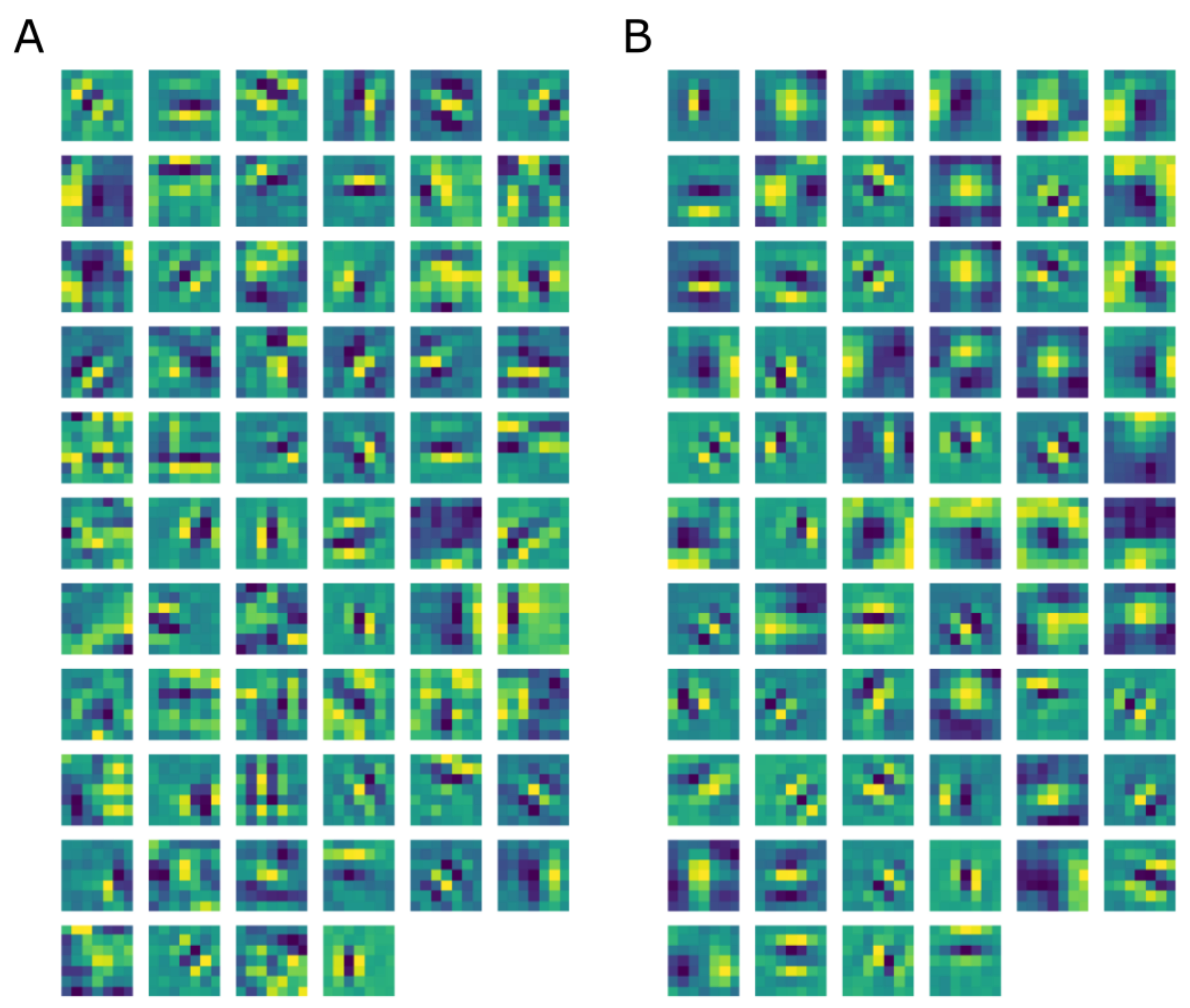
Figure 4: (A) Learned filters of $\ell^{1}$ of our CNN architecture. (B) Learned filters of $\ell^{1}$ of the same CNN architecture, but without $\ell^{0}$.

The filters in $\ell^{1}$ were approximated by the Gabor function in Eq. (3), where all the parameters were found using the built-in function optimize.curve_fit from the Python library SciPy. The mean correlation between the selected filters and their Gabor approximations obtained using the built-in function corrcoef from the Python library NumPy is 92.61%.

We then split the filter bank w.r.t. the parity of their approximation, indicated by the parameter $\phi$, that was forced to be between $-\pi$ and $\pi$. Specifically, we labelled a filter as odd if $\frac{\pi}{4}<|\phi|<\frac{3\pi}{4}$, as even if $0<|\phi|<\frac{\pi}{4}$ or $\frac{3\pi}{4}<|\phi|<\pi$.

Figure 5 shows the odd filters and their Gabor approximations, rearranged w.r.t. the orientation $\theta$. In this case the orientation $\theta$ spans across the range $[0^{\circ},360^{\circ}[$, in order to correctly code for filters sharing the same direction but with opposite positive and negative lobes – and therefore having orientations differing by $180^{\circ}$.

Figure 6 shows the even filters and their Gabor approximations, rearranged w.r.t. the orientation $\theta$. In this case, the orientation $\theta$ spans across the range $[0^{\circ},180^{\circ}[$. For the sake of visualization, those filters whose central lobe had negative values were multiplied by -1.

In both scenarios, the orientation values are quite evenly sampled, allowing the neural network to detect even small orientation differences. Most of the filters have high frequencies, allowing them to detect thin boundaries, but some low-frequency filters are still present.

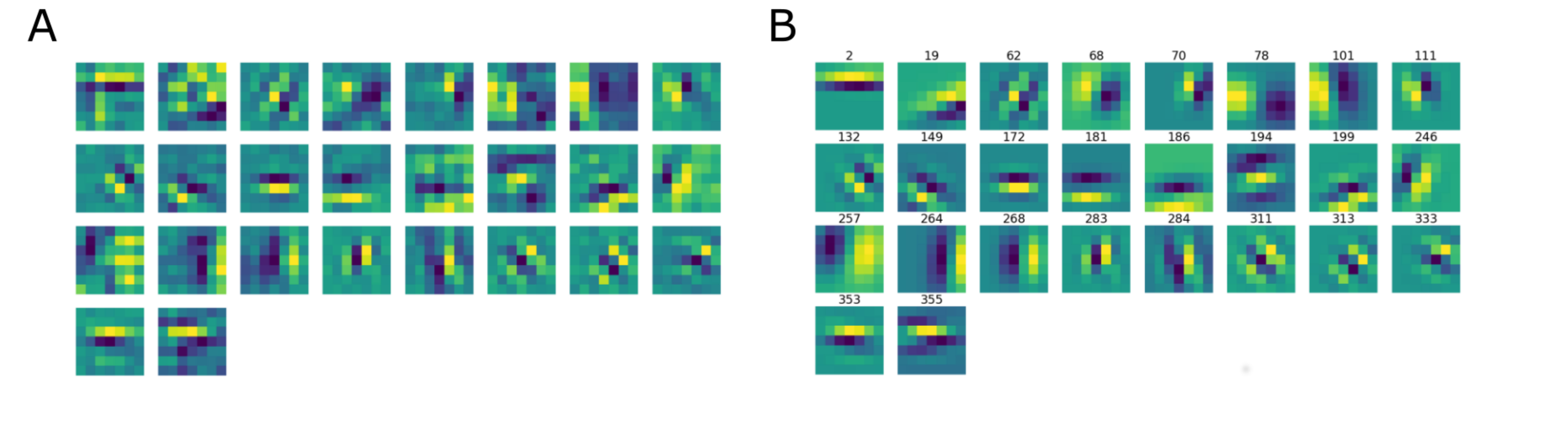
Figure 5: (A): the learned filters of $\ell^{1}$ with odd parity, ordered w.r.t. the orientation $\theta$ obtained from the Gabor approximation. (B): the approximating odd Gabor filters, labelled by their orientation.

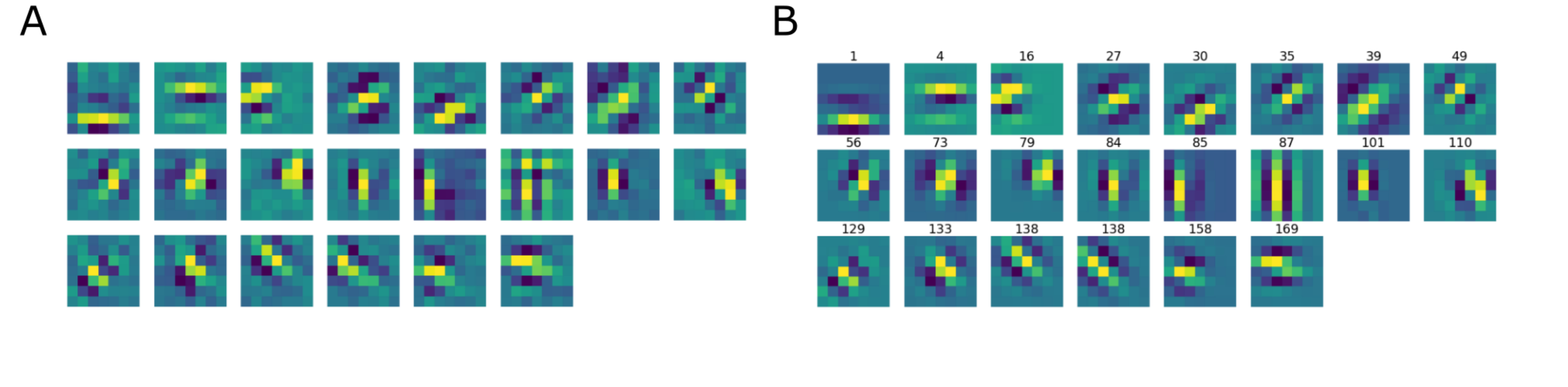
Figure 6: (A): the learned filters of $\ell^{1}$ with even parity, ordered w.r.t. the orientation $\theta$ obtained from the Gabor approximation. (B): the approximating even Gabor filters, labelled by their orientation.

6 Emergence of horizontal connectivity in the transition kernel

In this section, we shall examine the learned transition kernel $K^{1}$, to investigate whether it shows any invariances compatible with the known properties of the lateral connectivity of V1.

6.1 Re-parameterization of the connectivity kernel using the first layer approximation

In order to study the selectivity of the connectivity kernel to the properties of $\ell^{1}$ filters, we first rearranged it based on the set of coordinates in $\mathbb{R}^{2}\times S^{1}$ induced by the Gabor approximation of the filters.

We first split the kernel w.r.t. the parity of $\ell^{1}$ filters, resulting in two separate connectivity kernels for even and odd filters. We then adjusted the spatial coordinates of each kernel using the estimated Gabor filter centers $(x_{0},y_{0})$. Specifically, for each $f,g$ in $\{1,\ldots,n\}$, we shifted the kernel $K^{1}(\cdot,\cdot,f,g)$ of Eq. (8) so that a displacement of $(i,j)=(0,0)$ corresponds to the situation where the centers of the filters $\Psi_{f}$ and $\Psi_{g}$ coincide. Finally, the original ordering of $f,g$ in $\{1,\ldots,n\}$ has no geometric meaning. However, each filter $\Psi_{f}$ is now associated with an orientation $\theta_{f}$ obtained from the Gabor approximation. Therefore, we rearranged the slices of $K^{1}$ so that the $f$ and $g$ coordinates were ordered by the corresponding orientations $\theta_{f}$ and $\theta_{g}$. By fixing one filter $\Psi_{f}$, we then obtained a 3-D kernel

$$(i,j,g)\mapsto K^{1}(i,j,f,g)$$ (9)

defined on $\mathbb{R}^{2}\times S^{1}$, describing the connectivity between $\Psi_{f}$ and all the other $\ell^{1}$ filters with the same parity properties, each shifted by a set of local displacements $(i,j)\in\{-6,\ldots,6\}\times\{-6,\ldots,6\}$.

6.2 Association fields induced by the connectivity kernel

Starting from the re-parameterized kernel centered around a filter $\Psi_{f}$ as in Eq. (9), we used the $\theta$-coordinates to construct a 2-D association field as in Sanguinetti et al., (2010). We first defined a 2-D vector field by projecting down the orientation coordinates weighted by the kernel values. Specifically, for each spatial location $(i,j)$, we defined

$$V(i,j):=\max_{g}K^{1}(i,j,f,g)\>\cdot\>\frac{\sum_{g=1}^{n}K^{1}(i,j,f,g)v_{g}}{\|\sum_{g=1}^{n}K^{1}(i,j,f,g)v_{g}\|},$$ (10)

where $v_{g}\in\mathbb{R}^{2}$ is a unitary vector with orientation $\theta_{g}$. This yields for each point $(i,j)$ a vector whose orientation is essentially determined by the leading $\theta$ values in the fiber, i.e. the ones were the kernel has the highest values. The norm of the vector is determined by the maximum kernel value over $(i,j)$. Finally, we defined the association field as the integral curves of the so-obtained vector field $V$ starting from points along the trans-axial direction in a neighborhood of $(0,0)$.

Figure 7B shows the association field obtained from the kernel computed around the even filter $\Psi_{f}$ in Figure 7A, with orientation $\theta_{f}=138^{\circ}$. The vector field $V$ was plotted using the Matlab function quiver, and the integral curves were computed using the Matlab function streamline. The vectors and curves are plotted over a 2-D projection of the kernel obtained as follows. The kernel was first resized by a factor of 10 using the built-in Matlab function imresize for better visualization, and then projected down on the spatial coordinates by taking the maximum over $g$. Note that around $(0,0)$ the field is aligned with the orientation of the starting filter $\Psi_{f}$, while it starts to rotate when it moves away from the center – consistently with the typical shape of psychophysical association fields, see Section 2.2.

We also outline the similarity with the integral curves of Sanguinetti et al., (2010), see Figure 1D. However, in our case the rotation is less evident since the spatial displacement encoded in the kernel $K^{1}$ is more localized than the edge co-occurrence kernel constructed in Sanguinetti et al., (2010).

Figure 7C shows in red the approximation of each integral curve as a circular arc, obtained by fitting the parameter $k$ of Eq. (6) to minimize the distance between the two curves. The empirical curves induced by the learned connectivity kernel were very close to the theoretical curves, with a mean Euclidean distance of $0.0099$.

Figure 7: (A) The $7\times 7$ even filter $\Psi_{f}$, with orientation $\theta_{f}=138^{\circ}$. (B) The vector field $V$ and its integral curves obtained from the kernel of even filters computed around $\Psi_{f}$, with $\theta_{f}=138^{\circ}$. (C) The association field of the transition kernel of even filters (blue), and its approximation using the integral curves defined in (6) (red). For better visualization the kernel has been resized by a factor of 10 using the built-in Matlab function imresize.

6.3 Comparison of transition kernel with the solution of heat equation

In section 2.2 we recalled the relationship between connectivity kernel and the fundamental solution of Sub-Riemannian operators. In analogy with this remark, we compare the learned transition kernel $K^{1}$ with the fundamental solution of the sub-Riemannian heat equation in $\mathbb{R}^{2}\times S^{1}$

$$\frac{\partial u}{\partial t}=-\alpha\Delta_{X_{1},X_{2}}u=-\alpha\left(X_{1}^{2}u+X_{2}^{2}u\right),$$ (11)

where the sub-Laplacian operator is generated by the vector fields introduced in Citti and Sarti, (2006) and defined by Eq. (5). To this end, we fitted the parameter $\alpha$ by comparing the vector field $V$ generated from the kernel $K^{1}$ with the 2-D vector field obtained with the same procedure from the fundamental solution of (11). More precisely, the optimal parameter $\alpha$ was chosen as the one minimizing the mean angular difference between the two vector fields. We obtained an optimal value $\alpha=2.74$, with a mean angular difference of $0.0154$. Figure 8A shows the vector field $V$ in blue, and the sub-Riemannian vector field with optimal $\alpha$ in red. As remarked above, the kernel $K^{1}$ captures the connections over a localized spatial area. Figure 8B shows in green the sub-Riemannian vector field over a wider spatial region, with the local area that best fits the vector field $V$ highlighted in red.

The 3-D counterpart of this visualization is shown in Figure 9A, displaying two isosurfaces of the sub-Riemannian kernel, whereas the Figure 9B shows an isosurface of $K^{1}$. The geometry of the learned kernel $K^{1}$ is qualitatively similar to the local behavior of the theoretical kernel, shown by the red isosurface in Figure 9A.

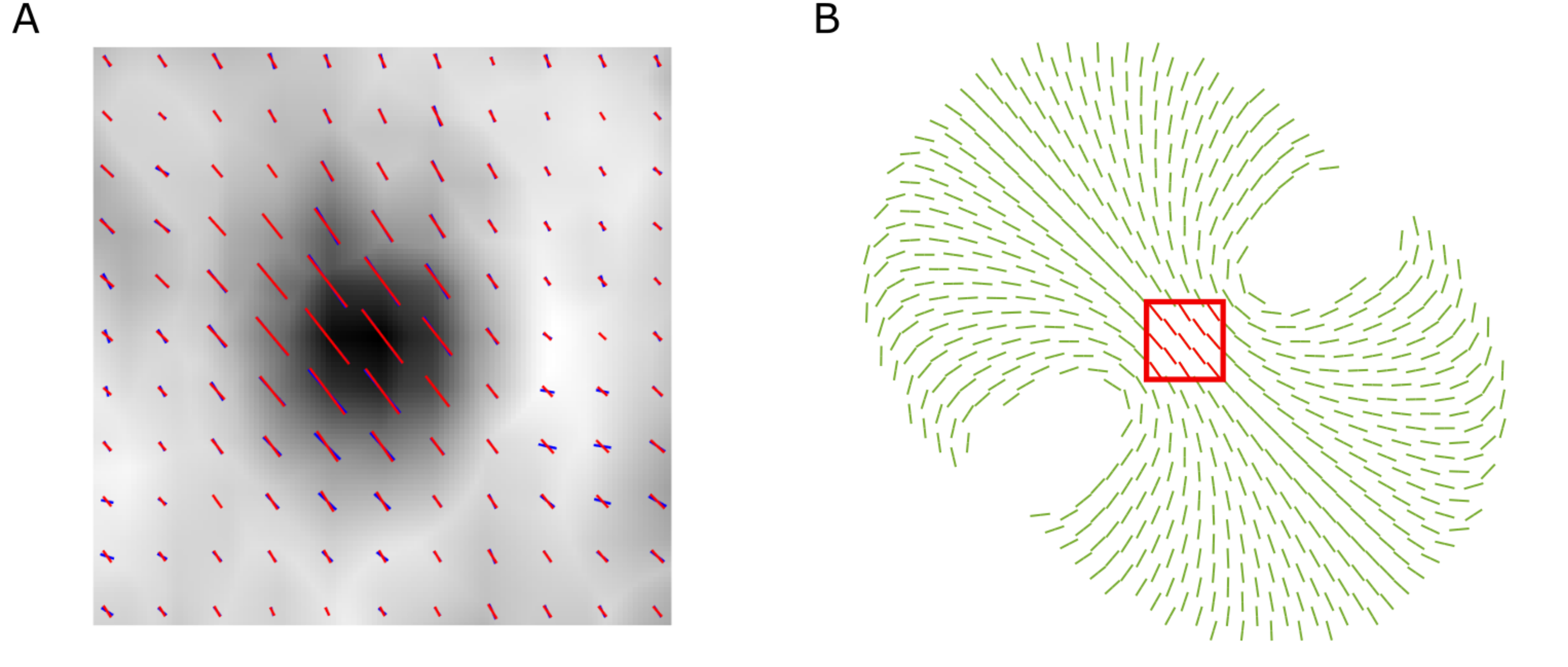
Figure 8: (A) In blue: the vector field of the transition kernel of even filters around $\Psi_{f}$. In red: the vector field of the best-fitting fundamental solution of the sub-Riemannian heat equation, with $\alpha=2.74$. (B) In green: the vector field of the best-fitting fundamental solution of the sub-Riemannian heat equation over a wider spatial region. In red: the local vector field fitted to the learned kernel.

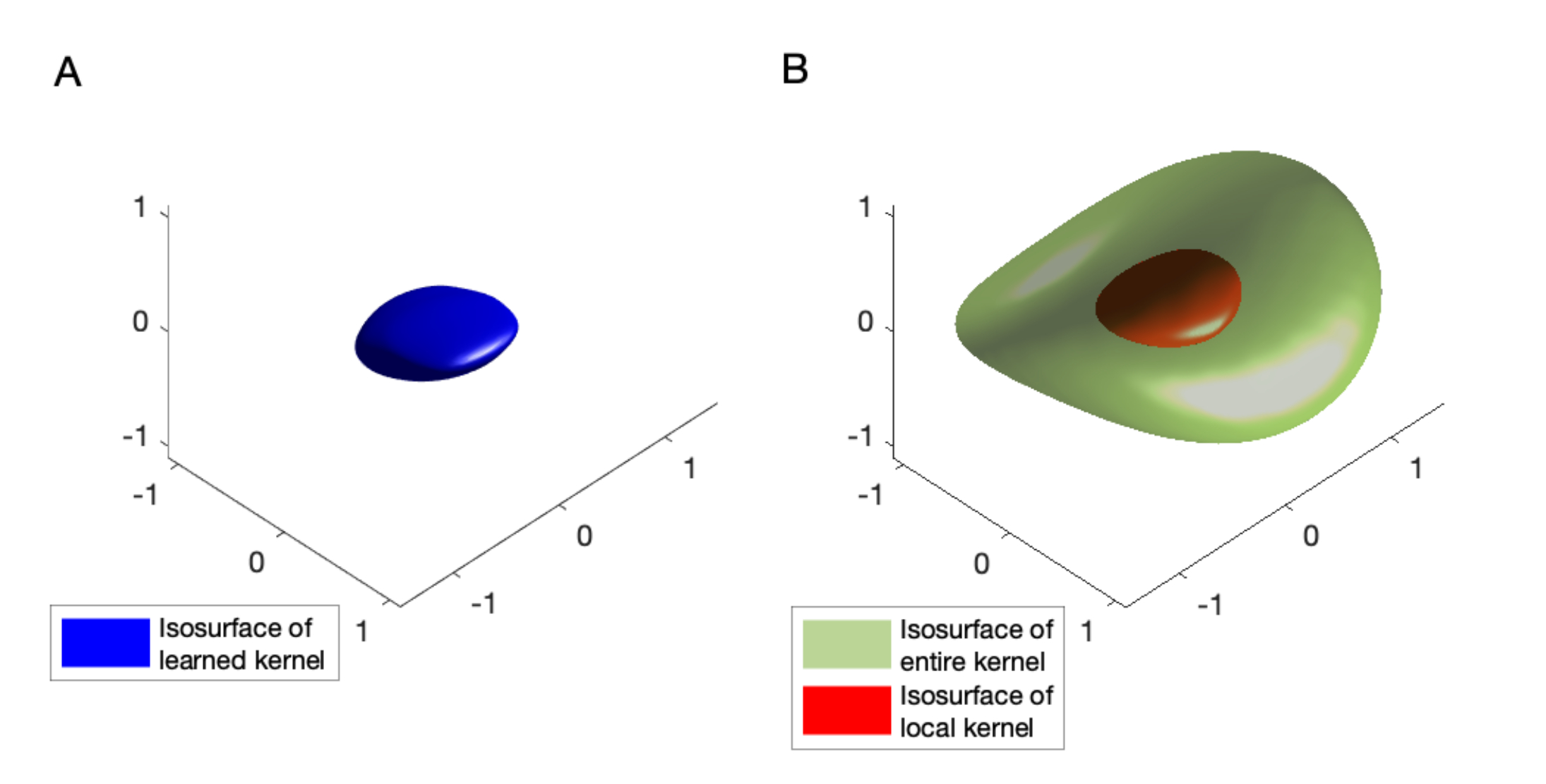
Figure 9: (A) Isosurface of the transition kernel $K^{1}$. (B) Isosurfaces of heat equation solution. In green: isosurface of the entire solution. In red: isosurface of the local solution. As expected the transition kernel is closer to this local isosurface.

7 Discussion

In this work, we showed how approximate group invariances arise in the early layers of a biologically inspired CNN architecture during learning on natural images, and we established a parallel with the architecture and plasticity of the early visual pathway. First, the LoG-shaped filter emerging in the pre-filtering stage $\ell^{0}$ closely resembles the typical LGN receptive profile exhibiting a rotational symmetry. The presence of $\ell^{0}$ also enhanced the orientation tuning of first-layer filters, thus separating the first image elaboration into two steps that may be roughly associated with sub-cortical and early cortical processing. Moreover, the introduction of lateral connections in the first network layer allowed us to investigate the relationship between the geometry of the feedforward filters and the selectivity of the learned connectivity kernel $K^{1}$. Indeed, the Gabor approximation of first layer filters provided us with a set of coordinates to re-map the kernel $K^{1}$ into the $\mathbb{R}^{2}\times S^{1}$ feature space, thus allowing to express the connectivity strength in terms of relative positions and orientations of the filters. Strikingly, the association fields induced by the learned connectivity bear a close resemblance to those obtained from edge co-occurrence in natural images by Sanguinetti et al., (2010), as well as to the flow of neural activity described by a sub-Riemannian heat equation in the Lie group setting introduced by Citti and Sarti, (2006).

We stress that such geometric properties arose spontaneously during the training of the CNN architecture on a dataset of natural images, the only constraint being the translation-invariance imposed by the convolutional structure of the network.

As future perspectives, we would like to extend our study by considering a wider range of features – possibly leading to a finer characterization of the geometry of first layer filters, including more complex types of receptive profiles. Moreover, considering a larger images dataset would make it possible to examine horizontal connectivity patterns spread over a wider spatial region. Finally, another direction could be to extend our model by comparing the properties of deeper network layers to the processing in higher cortices of the visual system.

References

- Abbasi-Sureshjani et al., (2018) Abbasi-Sureshjani, S., Favali, M., Citti, G., Sarti, A., and ter Haar Romeny, B. M. (2018). Curvature integration in a 5d kernel for extracting vessel connections in retinal images. IEEE Trans Image Process, 27:606–621.
- Anselmi et al., (2014) Anselmi, F., Leibo, J. Z., Rosasco, L., Mutch, J., Tacchetti, A., and Poggio, T. (2014). Unsupervised learning of invariant representations in hierarchical architectures.
- Barbieri et al., (2014) Barbieri, D., Cocci, G., Citti, G., and Sarti, A. (2014). A cortical-inspired geometry for contour perception and motion integration. J Math Imaging Vis, 49(3):511–529.
- Bertoni et al., (2019) Bertoni, F., Citti, G., and Sarti, A. (2019). LGN-CNN: a biologically inspired CNN architecture. Preprint available at https://arxiv.org/abs/1911.06276.
- Bosking et al., (1997) Bosking, W., Zhang, Y., Schoenfield, B., and Fitzpatrick, D. (1997). Orientation selectivity and the arrangement of horizontal connections in tree shrew striate cortex. J Neurosci, 17:2112–2127.
- Bressloff and Cowan, (2003) Bressloff, P. C. and Cowan, J. D. (2003). The functional geometry of local and long-range connections in a model of V1. J Physiol Paris, 97(2-3):221–236.
- Citti and Sarti, (2006) Citti, G. and Sarti, A. (2006). A cortical based model of perceptual completion in the roto-translation space. Journal of Mathematical Imaging and Vision archive, 24:307–326.
- Daugman, (1985) Daugman, J. G. (1985). Uncertainty relation for resolution in space, spatial frequency, and orientation optimized by two-dimensional visual cortical filters. J Opt Soc Am A2, 2:1160–1169.
- Ernst et al., (2007) Ernst, U., Deneve, S., and Meinhardt, G. (2007). Detection of gabor patch arrangements is explained by natural image statistics. BMC Neuroscience - BMC NEUROSCI, 8.
- Field et al., (1993) Field, D. J., Hayes, A., and Hess, R. F. (1993). Contour integration by the human visual system: evidence for a local association field. Vision Res, 33:173–193.
- Girosi et al., (1995) Girosi, F., Jones, M., and Poggio, T. (1995). Regularization Theory and Neural Networks Architectures. Neural Computation, 7(2):219–269.
- Hoffman, (1989) Hoffman, W. (1989). The visual cortex is a contact bundle. Appl Math Comput, 32:137–167.
- Hubel, (1987) Hubel, D. H. (1987). Eye, brain, and vision. New York, WH Freeman (Scientific American Library).
- Hubel and Wiesel, (1962) Hubel, D. H. and Wiesel, T. N. (1962). Receptive fields, binocular interaction and functional architecture in the cat visual cortex. J Physiol (London), 160:106–154.
- Hubel and Wiesel, (1977) Hubel, D. H. and Wiesel, T. N. (1977). Ferrier lecture: Functional architecture of macaque monkey visual cortex. Proceedings of the Royal Society of London. Series B, Biological Sciences, 198(1130):1–59.
- Koenderink and van Doom, (1987) Koenderink, J. J. and van Doom, A. J. (1987). Representation of local geometry in the visual system. Biol. Cybern., 55(6):367–375.
- Krizhevsky, (2009) Krizhevsky, A. (2009). Learning multiple layers of features from tiny images. Technical report.
- Lawrence et al., (1997) Lawrence, S., Giles, C. L., Tsoi, A. C., and Back, A. D. (1997). Face recognition: a convolutional neural-network approach. IEEE Transactions on Neural Networks, 8:98–113.
- LeCun et al., (1998) LeCun, Y., Bottou, L., Bengio, Y., and Haffner, P. (1998). Gradient-based learning applied to document recognition. In Proceedings of the IEEE, volume 86, pages 2278–2324.
- Lee, (1996) Lee, T. S. (1996). Image representation using 2d Gabor wavelets. IEEE Transactions on Pattern Analysis and Machine Intelligence, 18.
- Liang and Hu, (2015) Liang, M. and Hu, X. (2015). Recurrent convolutional neural network for object recognition. CVPR.
- Montobbio et al., (2019) Montobbio, N., Bonnasse-Gahot, L., Citti, G., and Sarti, A. (2019). Kercnns: biologically inspired lateral connections for classification of corrupted images. CoRR, abs/1910.08336.
- Montobbio et al., (2020) Montobbio, N., Sarti, A., and Citti, G. (2020). A metric model for the functional architecture of the visual cortex. Journal on Applied Mathematics, 80:1057–1081.
- Paszke et al., (2017) Paszke, A., Gross, S., Chintala, S., Chanan, G., Yang, E., DeVito, Z., Lin, Z., Desmaison, A., Antiga, L., and Lerer, A. (2017). Automatic differentiation in pytorch. In NIPS-W.
- Petitot, (2008) Petitot, J. (2008). Neurogéométrie de la vision - Modèles mathématiques et physiques des architectures fonctionnelles. Éditions de l’École Polytechnique.
- Petitot and Tondut, (1999) Petitot, J. and Tondut, Y. (1999). Vers une neuro-géométrie. Fibrations corticales, structures de contact et contours subjectifs modaux. In Mathématiques , Informatique et Sciences Humaines, volume 145, pages 5–101. CAMS, EHESS.
- Poggio and Anselmi, (2016) Poggio, T. and Anselmi, F. (2016). Visual Cortex and Deep Networks: Learning Invariant Representations. The MIT Press, Cambridge, MA, USA.
- Sanguinetti et al., (2008) Sanguinetti, G., Citti, G., and Sarti, A. (2008). Image completion using a diffusion driven mean curvature flowin a sub-riemannian space. volume 2, pages 46–53.
- Sanguinetti et al., (2010) Sanguinetti, G., Citti, G., and Sarti, A. (2010). A model of natural image edge co-occurrence in the rototranslation group. J Vis, 10.
- Sarti and Citti, (2015) Sarti, A. and Citti, G. (2015). The constitution of visual perceptual units in the functional architecture of V1. Journal of Computational Neuroscience, 38:285–300.
- Sarti et al., (2008) Sarti, A., Citti, G., and Petitot, J. (2008). The symplectic structure of the primary visual cortex. Biol. Cybern., 98(1):33–48.
- Serre et al., (2007) Serre, T., Wolf, L., Bileschi, S., Riesenhuber, M., and Poggio, T. (2007). Robust object recognition with cortex-like mechanisms. IEEE Transactions on Pattern Analysis and Machine Intelligence, 29(3):411–426.
- Sherstinsky, (2020) Sherstinsky, A. (2020). Fundamentals of recurrent neural network (rnn) and long short-term memory (lstm) network. Physica D: Nonlinear Phenomena, 404:132306.
- Spoerer et al., (2017) Spoerer, C., McClure, P., and Kriegeskorte, N. (2017). Recurrent convolutional neural networks: a better model of biological object recognition. Frontiers in psychology, 8:1551.
- Wilson and Cowan, (1972) Wilson, H. R. and Cowan, J. D. (1972). Excitatory and inhibitory interactions in localized populations of model neurons. Biophys J, 12(1):1–24.
- Yamins et al., (2015) Yamins, D., Hong, H., Cadieu, C., and Dicarlo, J. (2015). Hierarchical modular optimization of convolutional networks achieves representations similar to macaque it and human ventral stream. Advances in Neural Information Processing Systems.
- Yamins and DiCarlo, (2016) Yamins, D. L. K. and DiCarlo, J. J. (2016). Using goal-driven deep learning models to understand sensory cortex. Nature Neuroscience, 19:356 – 365.