The challenges of temporal alignment on Twitter during crises

Abstract

Language use changes over time, and this impacts the effectiveness of NLP systems. This phenomenon is even more prevalent in social media data during crisis events where meaning and frequency of word usage may change over the course of days. Contextual language models fail to adapt temporally, emphasizing the need for temporal adaptation in models which need to be deployed over an extended period of time. While existing approaches consider data spanning large periods of time (from years to decades), shorter time spans are critical for crisis data. We quantify temporal degradation for this scenario and propose methods to cope with performance loss by leveraging techniques from domain adaptation. To the best of our knowledge, this is the first effort to explore effects of rapid language change driven by adversarial adaptations, particularly during natural and human-induced disasters. Through extensive experimentation on diverse crisis datasets, we analyze under what conditions our approaches outperform strong baselines while highlighting the current limitations of temporal adaptation methods in scenarios where access to unlabeled data is scarce.

1 Introduction

Patterns of language use change constantly over time, often in predictable and analyzable ways Hamilton et al. (2016a); Kulkarni et al. (2015); Sommerauer and Fokkens (2019). As language changes, the performance of NLP systems can be negatively impacted Lazaridou et al. (2021). In most scenarios, training corpora are derived from a snapshot of data at some moment of time in the past, which puts the reliability of model performance on future data into question. Yet, there lacks a concrete reasoning or evidence that temporal adaptation elevates model performance. Despite the popularity of large language models and their usefulness in many NLP domains (Devlin et al., 2019), the representation of temporal knowledge in those models so far remains an open challenge.

The increased interest in temporal adaptation (i.e. scenarios in which the training and test datasets are drawn from different periods of time) has led to the curation of a number of datasets such as NYT Annotated Corpus (Sandhaus, 2008) and Amazon Reviews (Ni et al., 2019) that have been the focus of most of the recent work in this area. However, these benchmark datasets are curated in such a way that they can only capture temporal change of language over long periods of time (from years to decades), giving access to a large amount of data. In the contrary, on social media, language changes can happen rapidly (Kulkarni et al., 2015; Eisenstein, 2013). Word usage and topics can even change over the span of a single day (Golder and Macy, 2011), especially during very dynamic scenarios like crisis or disastrous events (Reynolds and Seeger, 2005; Del Tredici et al., 2019). We denote these phenomena induced by linguistic and semantic changes over time as temporal drift.

Accounting for temporal drift is critical in crisis situations in which information patterns can vary greatly between the phases of emergency management for crisis. For this purpose, we study short text classification in crisis situations. Given the time-critical nature of crisis scenarios, gathering annotations is too time-consuming and transfer learning is challenging due to the innate differences among the type of events (hurricane vs. earthquake) and the respective information needs. Thus, we offer a study investigating the impact of temporal drift on crisis datasets spanning shorter time periods (days/weeks), as well as datasets with relatively few samples (ranging from $\sim$1k to 22k).

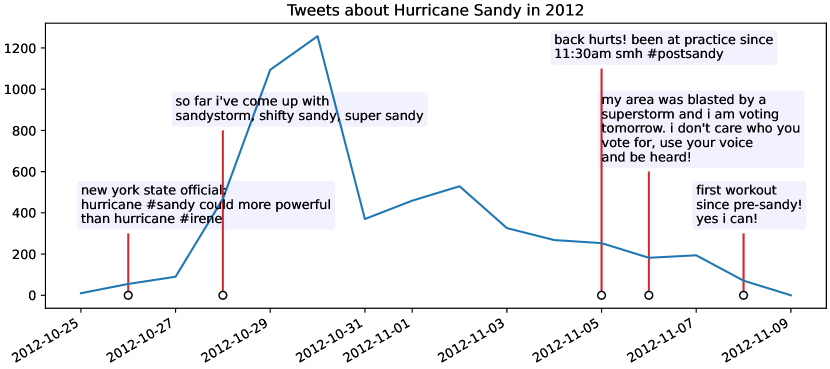
Figure 1: The blue line indicates the frequency of tweets during the hurricane Sandy Stowe et al. (2018). The displayed tweets demonstrate challenging linguistic phenomena for a text classification model, e.g. semantic shifts (#irene as reference to a hurricane rather than a person) or neologisms (pre-sandy).

Assessing rapid temporal drift is a challenging problem due to different linguistic phenomena which often require extensive knowledge about the temporal structure of the context. In Figure 1, we provide examples from Stowe et al. (2018) dataset, which were collected from the 2012 New York City landfall of Hurricane Sandy.

Existing approaches like continual learning Gururangan et al. (2020); Loureiro et al. (2022a) or learning time-specific models Agarwal and Nenkova (2022) cannot be applied to this scenario as access to a large set of unlabeled data from the temporal target distribution is missing. Unlike existing approaches, which react to incoming annotated data to update their models, we use temporal metadata as a training signal such that the existing contextualized representations are adapted temporally. More specifically, we are the first to apply projection methods (Wang et al., 2014) and domain adaptation approaches (Ganin et al., 2016; Bamler and Mandt, 2017) to learn time-aware contextualized embeddings. Our results highlight the challenges of integrating temporal information into contextualized embeddings with improvements being dependent on factors like dataset size - and thereby emphasizing that temporal adaptation remains a challenge in scenarios where we do not have access to large unlabeled data.

In summary, we make the following contributions:

1. We investigate temporal drift during crisis events and its adversarial effect on task performance. To the best of our knowledge, this is the first study of temporal effects on text classification performance in crisis scenarios, when temporal drift is rapid and access to data is scarce.

2. We investigate the role of the domain of data in temporal drift and propose a simple metric to quantify the impact of temporal degradation on task performance.

3. We propose methods that adapt future data to known models, improving performance with no additional labeled data.

4. Through experiments on a multitude of diverse text classification datasets collected during crisis events, we analyse the effectiveness of our proposed methods over strong baselines.

2 Related Work

Analyzing semantic change of text over time has been of great interest since the pioneering work by  Hamilton et al. (2016b) and others (Kutuzov et al., 2018; Rudolph and Blei, 2018; Martinc et al., 2020; Gonen et al., 2020). However, its influence on downstream task performance has only recently gained attention. Most importantly, the advent of contextualized word embeddings and large pretrained language models has led researchers to re-evaluate the role of temporality in language modeling (Jawahar and Seddah, 2019; Lazaridou et al., 2021; Hofmann et al., 2021; Kulkarni et al., 2021) and text classification (Bjerva et al., 2020; Florio et al., 2020; Röttger and Pierrehumbert, 2021; Agarwal and Nenkova, 2022).

The performance degradation due to temporal factors has been confirmed in several studies and across multiple domains. Jaidka et al. (2018) analyzed the temporal performance degradation of age and gender classification models based on user’s social media posts. Based on features derived from Latent Dirichlet Allocation and word embeddings, they find that models perform best if test and training data come from the same time span. Florio et al. (2020) investigated temporal effects on Hate Speech detection in Italian social media over the period of five months. Their results suggest that models trained on data temporally closer to the test data perform better with transformer based models. Loureiro et al. (2022b) studied semantic shifts in social media and proposed a dataset annotated with words that have undergone a semantic shift over the past two years. Loureiro et al. (2022a) focus on Twitter as text domain and contribute pretrained language models which have been further trained on time-specific data from Twitter.

Bjerva et al. (2020) propose to use sequential subspace alignment (SSA) to adapt contextualized word embeddings for language change over time. Their results suggest that SSA applied on past data is able to outperform baselines which have access to data from all time-steps. Röttger and Pierrehumbert (2021) compared time-agnostic domain adaptation with temporal domain adaptation which considers the temporal order of the data. They found that, while temporal adaptation clearly outperforms domain adaptation in language modeling, this does not necessarily translate onto downstream classification performance due to updated tokens not being relevant for the task. Agarwal and Nenkova (2022) found the temporal model performance deterioration to be less significant when using language representations which have been pretrained on temporally closer data.

Finally, Luu et al. (2022) have made the effort of conducting a large-scale study of temporal misalignment, the generalized scenario where training and evaluation data are drawn from different periods of time. Across multiple NLP classification tasks and domains they identify performance degradation with varying degrees but with social media and news being the most affected domains.

We contribute to the existing line of work by quantifying the temporal effects on downstream task performance over short time periods (days and weeks) during crisis events. In such a scenario and in contrast to previous work, we do not assume access to large corpora of unlabeled data for temporal adaptation via continuous pretraining. Our proposed approaches temporally adapt pretrained contextualized embeddings to learn time-aware embeddings and we evaluate their effects on downstream classification tasks.

3 Methods Overview

Luu et al. (2022) describe three distinct stages of a typical NLP system which consist of a pretraining stage, a domain (or temporal) adaptation stage and a fine-tuning stage. Separating the adaptation and fine-tuning stages makes the implicit assumption that there is access to unlabeled data from the (temporal) target distribution which has been proven to be beneficial for temporal adaptation (Luu et al., 2022). In contrast, we are looking at the dynamic setting during crisis events. Temporal alignment through continuous pre-training is not feasible due to the lack of unlabeled data and time constraints imposed by the application scenario (e.g. crisis monitoring). The latter also limits the feasibility of an online learning setup which requires new annotations in a continuous stream. Finally, transfer learning is difficult due to inherent differences in information needs (i.e. the type of labels) and domains (e.g. hurricane vs. earthquake).

Therefore, in this section we adapt and evaluate methods which are specifically designed for combining temporal adaptation and fine-tuning. Their training procedures are adapted to incorporate temporal information about the data along with the textual input. We describe each approach in the following:

Adapted Language Modelling (ALM)

Similar to previous work (see Section 2), we explore temporal adaptation via pretraining but use only the available training data. We therefore continue with the language modeling objective of our respective pretrained language model on the training data and use the resulting fine-tuned model (FT) for downstream task training. Following Dhingra et al. (2022), we investigate a variation for temporal modelling (TM) by concatenating time as textual information to the input to encourage the language model to learn temporally relevant features during pretraining.

DCWE: Dynamic Contextualized Word Embeddings

Hofmann et al. (2021) introduced a principled way to impart extra-linguistic knowledge into contextualized word embeddings by involving a prior distribution. This enables us to integrate temporal information into the embeddings during training. More specifically, for each temporal snapshot (e.g. days, months, years, etc.) present in the training data, an additional set of parameters is learned which acts as a temporal offset added to the original word embeddings. This way the model is able to maintain the semantic meaning of a word embedded in its temporal context. We adapt this idea to our setting by introducing additional parameters for shifting the pre-trained contextualized embeddings. Given a sequence of words/tokens $W=[w_{1},w_{2},...,w_{n}]$ and their corresponding pre-trained embeddings $H=[h_{1},h_{2},...,h_{n}]$. To account for the temporal effect on the word meanings, we model word embeddings as a function of temporal context $t$ associated to $W$.

$$h^{*}_{i}=f(h_{i},t)$$ (1)

Since meanings of most of the words in the vocabulary are temporally stable, we can place a Normal prior on $h^{*}_{i}$.

$$h^{*}_{i}\sim\mathcal{N}(h_{i},\lambda^{-1}I)$$ (2)

Hence, we write as $h^{*}_{i}=h_{i}+d_{i}$, where the offset $d_{i}$ is normally distributed as $d_{i}\sim\mathcal{N}(0,\lambda^{-1}I)$. However, pre-trained LMs make this temporal adaptation easily applicable to any task by adding only a regularization term $L_{temporal}$ on top of the task specific loss $L_{task}$.

$$L_{temporal}=\frac{\lambda}{n}\sum_{i=1}^{n}(||d_{i}||_{2}^{2}+K||d_{i}-d_{i-1}||_{2}^{2})$$ (3)

For training the model, the overall loss $L=L_{task}+L_{temporal}$ is minimized. Similarly to Hofmann et al. (2021), we use $K=10^{3}$ from Bamler and Mandt (2017), to enforce that $h^{*}_{i}$ s change smoothly over time.

LMSOC: Socio-temporally Sensitive Language Modeling

Similar to DCWE, Kulkarni et al. (2021) propose a method to learn extra-linguistic context using graph representation learning algorithms and then primes with language models to generate language representations grounded in a socio-temporal context. We model the temporal order information as a linear chain graph and adapt this method to our setting by appending temporal graph embeddings to the initial layers of the pre-trained language model. During fine-tuning of the language model, the graph embeddings are kept frozen to inductively yield temporally-aware embeddings.

TAPH: Time Aware Projection on Hyperplanes

Time adds an additional context or dimension to the knowledge making temporal scoping an imperative part while deriving context embeddings. Therefore, we model temporal information as a hyperplane and define a projection operation (Wang et al., 2014) on it. To build a time-invariant classification model, we project the sentence-embedding (Reimers and Gurevych, 2019) of each text on a hyperplane to obtain a time-aware sentence embedding. We describe the method in more detail.

Let $X=[x_{1},x_{2},...,x_{n}]$ be a given sequence of words and $H$ be its sentence embedding. Since the temporal span of our data is short, we assume that the temporal hyperplane $w_{t}$ represents the time frame of the training data. We derive time-aware sentence embeddings $H_{t}$ using our defined projection operation as follows:

$$H_{t}=H-w_{t}^{\intercal}Hw_{t}$$ (4)

While training the model, we learn the hyperplane representation $w_{t}$ in addition to fine-tuning the pre-trained embeddings in an end-to-end fashion. However during inference, we assume that we could ‘teleport’ the data to the past by projecting their sentence embeddings on the hyperplane $w_{t}$ in order to revert their temporal changes. We then use these embeddings in the downstream tasks.

TDA: Temporal Domain Adaptation

Temporal Adaptation can also be interpreted as a variant of domain adaptation with the difference that the language change happens within the same domain, e.g. induced by external events or the general dynamic characteristics of the source infrastructure (e.g. social media platforms or news outlets). We adapt a widely used domain adaptation method (Ramponi and Plank, 2020) to our setting. We learn time-aware word representations by adding an additional classification layer during training to predict the time of each text and apply the Gradient Reversal method (Ganin et al., 2016). In this way, the input does not change during the forward pass but this additional layer affects the model parameters during back-propagation of error by an additional penalizing factor. This acts as an adversarial training objective forcing the model to adapt to the temporal structure of the data.

4 Experimental Setup

4.1 Data

We identify a collection of social media data during crisis with observable temporal phases (pre-, acute- and post-crisis), rapid change in language and a natural change in distribution over time - enabling us to evaluate how well temporally adapted models generalize over time. We use three datasets sampled from Twitter: Sandy, T26, and Humaid. We provide an overview here and refer to the Appendix A for dataset details.

Sandy

The dataset from Stowe et al. (2018) collected during hurricane Sandy in 2012 contains approximately 22,000 tweets spanning 17 days centered on landfall in New York City, annotated for binary relevance to the storm and its effects. The tweets were collected by first identifying users impacted by the event, then retroactively pulling their data from before, during, and after the event. As opposed to keyword collection, this provides a relatively broad collection of both relevant and non-relevant tweets and a more complete dataset for evaluating temporal drift, as each tweet doesn’t necessarily contain the same keyword(s).

T26

The CrisisLex T26 (T26) dataset Olteanu et al. (2015) includes labeled tweets for 26 different crisis events, labeled by informativeness into four different categories: (1) related to the crisis and informative, (2) related to the crisis but not informative, (3) not related to the crisis, and (4) not applicable category. This collection reflects a wide variety of events covering natural and human-created emergencies, with the added difficulty that the individual datasets are relatively small, with each event containing only approximately 1,000 tweets.

Humaid

The Humaid dataset (Alam et al., 2021) is similar to T26, containing data about 19 different events with dataset sizes ranging from 575 to 9467 tweets. They are annotated with 11 different classes designed to capture fine-grained information related to disaster events.

4.2 Data Splits

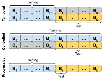
Figure 2: Overview of the data splits used in our experiments. Bins in blue are used during training, bins in yellow for testing, grey bins are not used. The progressive setting comprises multiple experiments with increasing training data size and a single test data bin moving forward temporally.

We follow previous work (Lazaridou et al., 2021; Agarwal and Nenkova, 2022) and create time-based data splits to assess the temporal performance degradation. Specifically, we use three variants of dataset splits: control, temporal and progressive. We illustrate this in Figure 2.

temporal Setup

First, we split the entire data into two halves which cover equally-sized time periods. We call these first temporal half and the second temporal half, respectively. In the temporal setting, we use all the data from the first temporal half as the training data and a test set which is comprised of a randomly sampled $50\%$ of data from the second temporal half of a dataset. This evaluates the model’s temporal generalization capabilities on test data from a temporally distant distribution than the training data.

control Setup

To assess whether temporal setup constrains model’s generalization capabilities, we compare its performance with a control setup. Here, we evenly spread the training data over time frames, exposing the model to the full knowledge of all time. In this setting, the training data comprises of $50\%$ of instances from the first temporal half, along with $50\%$ instances from the second temporal half, matching the total training data from the temporal setup. We use the same test set as in temporal setup while ensuring that there is no overlap between the train and test split from the second temporal half.

Under the assumption that a temporal gap between training and target distribution leads to performance decay, we expect that the control setup will yield better scores, as the model has access to training instances from the same temporal distribution as the test data.

progressive Setup

As described previously, semantic changes are likely to occur in short time spans within crisis-related data streams. Therefore, to investigate a more fine-grained analysis of temporal performance decay, we simulate a scenario in which an event is progressing, we have access to all the previous data, and need to take decisions about the incoming data. In this setup, we split the entire dataset into ten temporally ordered bins with even samples. Then, for each test bin $B_{t}$, we use all preceding bins $B_{0}$ to $B_{t-2}$ for training. To identify the best performing model across all training epochs, we use bin $B_{t-1}$ for development.

4.3 Baseline

For a consistent performance comparison, all proposed models use bert-base-cased as their underlying backbone model for deriving pre-trained embeddings.

For the FT setup (see Section 3), we use the available training data for each dataset to run masked language modelling for three epochs to adapt the model to the data. We then fine-tune for the downstream task on the relevant training data using the updated pre-trained model. This will indicate whether the domain is the issue, or whether there is additional temporal effects. In the temporal modeling setup (TM) setup, we follow Dhingra et al. (2022) and prepend the textual representation of the timestamp for each tweet to the tweet text, then train an additional three epochs of masked language modelling. We then fine-tune for the downstream task on the relevant training data.

Finally, we apply another baseline where we use the timestamp text as second input to the model during supervised training, separated via a special token (i.e. [SEP] for BERT). We refer to this baseline as SEP.

4.4 Hyperparameters and Infrastructure

For a fair comparison, we run all experiments using the same hyperparameters and data splits. We use a learning rate of $1e-4$, batch size of 64, weight decay of $1e-3$ and no warmup due to the limited amount of training data. We use Adam Loshchilov and Hutter (2019) as optimization algorithm and train for three epochs. Based on the performance on the development split, we load the best performing model at the end of the training procedure.

We repeat each experiment using five different seeds and take the most frequent prediction across all runs as the final prediction by a model. All models are implemented in Python 3.6 using PyTorch 1.10.2 (Paszke et al., 2019) and the HuggingFace (Wolf et al., 2020) framework (4.18) as model backend. We used a computation cluster containing a mixture of NVIDIA Tesla P100 (16GB), NVIDIA A100 (40GB) and NVIDIA V100 (32GB) GPUs.

4.5 Evaluation

We report binary-F1 Score for Sandy and macro-F1 score for multi-class classification task on T26 and Humaid datasets. The comparison of the control and temporal setting serves two purposes; first, to quantify the degradation of model performance due to temporal drift and second, to estimate the temporal adaptation ability for our approaches. We expect that models considering temporal information should experience less performance degradation between these two settings compared to the baseline model.

Additionally, we evaluate the mean model performance in the progressive setting for a more fine-grained analysis of temporal degradation.

Temporal Rigidity: While analyzing the effects of temporal drift on model performance, it is necessary to quantify the degradation of model performance due to this phenomenon. We quantify the temporal adaptability of a model using a metric called Temporal Rigidity (TR) score, that summarizes the performance deterioration of a model from aligned to misaligned test data. Higher values of TR imply that the model is not able to adapt itself temporally.

We denote $f_{M}(B_{i},B_{j})$ as the F1 performance score of a model $M$ when trained using data sampled from bin $B_{i}$ and evaluated using data sampled from bin $B_{j}$. We define TR as:

$$TR=\frac{1}{N}\sum_{i\neq j}{\frac{\lvert f_{M}(B_{i},B_{j})-f_{M}(B_{i},B_{i})\rvert}{\lvert i-j\rvert}}$$ (5)

In Eqn.5 the normalization factor is given as $N=\lvert\{(i,j):i\neq j\}\rvert$. Unlike Luu et al. (2022), who do not take temporal proximity of bins into account. We use $\frac{1}{\lvert i-j\rvert}$ as the penalizing factor for the model when training and test bins are temporally close but the performance degradation is significant.

Crisis Phases: Additionally, we utilize the well-known temporal structures of the crisis events (Reynolds and Seeger, 2005; Yang et al., 2013) to analyze model performance. The temporal structure of the Sandy dataset is annotated using pre-, acute- and post-crisis labels. For each model we cluster the time-aware embeddings using K-Means algorithm (k=3) and report the Normalized Mutual Information score (NMI). NMI gives the correlation between the time-aware embeddings and the temporal structure of the underlying data.

5 Results and Analysis

In this section, we attempt to answer the following questions:

1. To what degree is temporal performance degradation present in short-term Twitter data during crisis events? (Section 5.1)

2. Does temporal adaptation improve model performance? (Section 5.2)

3. Does the domain of the data play a role in temporal drift? (Section 5.3)

4. How do the proposed models perform when trained continually? (Section 5.4)

5.1 Temporal Performance Degradation

Data	Sandy	T26	Humaid
control - temporal	6.52	4.37	4.10

Table 1: Temporal Performance Degradation: Averaged F1 performance difference of the control to temporal setting for the BERT baseline model. Overall results show that contextualized language models fail to adapt temporally. Refer Section 5.1 for details.

In order to estimate the degree of temporal performance degradation in the crisis scenario, we compare the classification performance of the baseline model in the control and temporal setting. Table 1 provides the averaged performance difference for all datasets. Given that we only change the temporal distribution of the training data, the effect is substantial with a difference in F1 up to 6.52 points for the Sandy dataset and slightly less pronounced on the T26 (4.37) and Humaid (4.10) dataset collections. Therefore, we conclude that, even in short-term scenarios like crisis events on Twitter, temporal distribution of the training data influences the classification performance.

5.2 Performance Comparison

Method	Sandy
	cont	temp	diff
BERT	87.70	81.18	6.52
BERT+TM	82.55	70.48	12.07
BERT+SEP	87.79	79.65	8.14
BERT+LMSOC	73.78	67.24	6.54
BERT+DCWE	86.92	79.95	6.97
BERT+TAPH	87.40	82.02	5.38
BERT+TDA	87.10	82.53	4.57
BERTFT	86.96	81.84	5.12
BERTFT+LMSOC	74.89	67.90	6.99
BERTFT+DCWE	86.85	79.53	7.32
BERTFT+TAPH	87.12	82.60	4.52
BERTFT+TDA	86.71	83.43	3.28

Table 2: Temporal Adaptation Evaluation on Sandy: Text classification performance measured in binary F1. Overall, TDA outperforms other approaches in temporal  setting, with and without temporal adaptation (FT). Refer Section 5.2 and 5.3 for details.

Method	T26	Humaid
BERT+TM	4 / 26	3 / 19
BERT+SEP	5 / 26	3 / 19
BERT+DCWE	0 / 26	1 / 19
BERT+TAPH	6 / 26	0 / 19
BERT+TDA	10 / 26	4 / 19
BERTFT+DCWE	0 / 26	0 / 19
BERTFT+TAPH	5 / 26	0 / 19
BERTFT+TDA	8 / 26	0 / 19

Table 3: Performance Comparison on T26 and Humaid: The number of datasets for which the specific temporal adaptation method outperforms its baseline counterpart in the temporal setting. Refer Section 5.2 and 5.3 for details.

We summarize the results on Sandy in Table 2. Overall we find that TDA outperforms all other methods in temporal setting. We obtain around $1.6\%$ absolute increase over the baseline. We also observe that the difference between model performance in control and temporal setting (diff) is lowest for TDA ($30.8\%$ lower than the baseline) indicating the higher robustness of the model. TAPH achieves $1\%$ absolute improvement in performance over the baseline in temporal setting (diff is lower by $16.9\%$).

The T26 and Humaid datasets contain data for a multitude of events. Therefore, we aggregate model performances in Table 3 and provide detailed results per event in the Appendix A.2. We see that model performance varies greatly between the Sandy dataset and the others. This is due to two main reasons: (i) Data Size: Most of the event datasets in T26 and Humaid are very small, the temporal adaptation methods do not get enough training data to learn the parameters involved in temporal reasoning. To support our argument, we observe, in “Boston Bombings (2013)” dataset of T26, which contains 81,172 annotated tweets, TDA outperforms the baseline by an absolute increases of $6.17\%$ and TAPH comes second with an absolute performance improvement of $2.9\%$ under temporal setting, a performance pattern which is similar to Sandy dataset. (ii) Data Quality: Unlike Sandy, T26 and Humaid have been collected using keyword-based search. This data collection technique has two main drawbacks: firstly, it restricts the data size and secondly, harms the completeness of the dataset collecting tweets that contain same keywords. All the improvements we report are statistically significant ($p<0.05$, using McNemar’s Test).

Learning from Temporal Information: To understand the cause of the performance improvement of the models, we utilize the annotated temporal structure of the Sandy dataset. In Table 4 we report two additional metrics: TR Score and NMI, in temporal setting. Compared to the baseline, TDA is lowest ($15.74\%$ decrease) which suggests that TDA performs most robustly over time across all models. TAPH comes in second with a $9.26\%$ decrease in TR Score from the baseline. NMI scores show similar patterns, with TDA achieving the highest score. We conclude that TDA learns the most meaningful time-aware embeddings.

Method	Sandy
	TR	NMI
BERT	0.108	0.051
BERT+TM	0.130	0.050
BERT+DCWE	0.111	0.105
BERT+TAPH	0.098	0.185
BERT+TDA	0.091	0.194

Table 4: Temporal Information Learning: Comparison of methods on TR (lower is better) and NMI scores (higher is better). Refer section 5.2 for details.

5.3 Effect of Domain of Data

To understand whether the data domain is the main issue behind performance degradation or temporal effects indeed play a significant role, we perform additional experiments. We fine-tune the initial bert-base-cased embeddings for an additional three epochs with Masked Language Modeling Task (MLM) on the training data, before applying the Temporal Adaptation methods. We report the results for Sandy dataset in Table 2. For all models, there remains a substantial performance difference between the control and temporal settings which demonstrates the influence of temporal drift on performance. Similar to previous work (Agarwal and Nenkova, 2022), we observe that additional pre-training improves performance for most of the models. Still, TDA outperforms the baseline and TAPH comes in second.

5.4 Effect of Continual Learning:

Method	Sandy
BERT	68.67
BERT+TM	60.13
BERT+DCWE	67.39
BERT+TAPH	69.13
BERT+TDA	69.50

Table 5: Continual Learning Effects: Average model performance across all bins in progressive setting, in terms of F1 Score. Refer section 5.4 for details.

Continual Learning requires continuous annotation of incoming data, which is not feasible during crisis events. However, for the analytical completeness of this paper, we simulate continual learning in the progressive setting to show the effectiveness of our proposed methods. In this setting, initially the models get access to very small amount of data to learn from, which affects model performance. Performance improves as the size of training data increases gradually. In Table 5 we report the model performance averaged over all the bins. The results show that TDA outperforms and improves the BERT baseline by $1.2\%$.

6 Discussion

Figure 3: Representative example shows that in comparison with other models TDA correctly puts maximum attention weight on the word katrina (another storm) in the temporal context of the hurricane while computing the contextual embeddings. Refer Section 6 for details.

Adapting temporally by training on timestamp patterns as text prepended to the input (BERT+TM) underperforms in all experiments. We argue that the added information affects all tokens equally via the self-attention mechanism although only some tokens will experience a semantic shift relevant for text classification in the crisis scenario.

Similarly, the LMSOC and DCWE adaptation approaches cannot outperform the baseline without any temporal adaptation. The additional parameters for computing the temporal offset are not well-tuned for predicting temporal distributions which have not been observed during training.

Figure 3 shows that TDA correctly learns to put maximum attention weight on the word Katrina (i.e. reference to a previous hurricane) in the temporal context of hurricane. We provide representative examples of tweets in Appendix A that all other models but TDA fail to classify correctly. Forcing the model to learn time-invariant embeddings during training using an adversarial signal leads to TDA performing better over all other approaches. Although, TAPH does not fall far behind, it approximates temporal information to create time-static bins. The discrete approximation of temporal information is the main reason behind its performance drop.

7 Conclusion

The usage of natural language inevitably changes over time which influences performance of text classification models applied on data from different temporal distributions. We show that this effect is also prevalent for rapid temporal drift using social media during crisis events as an example. With the rise of pretrained contextualized embeddings, a dominant approach is to continue language modeling on data temporally closer to the target distribution. However, during crisis events such data is not available and annotated data is often scarce.

We investigate approaches which work without any additional data besides the input text and its temporal metadata. Our results show that under ideal conditions, i.e. high data quality and sufficient annotated instances, they outperform strong baselines. However, most crucially, our work highlights a critical gap of temporal adaptation for rapid temporal drift, namely if unlabeled data for alignment is missing and annotated data is scarce. Our work opens the door for future research on methods which do not rely on pretraining in unlabeled target domain data. In this sense, crisis data provides an interesting use case for evaluation. We release all our code and models, fostering future work in this area.

Limitations

While existing approaches account for temporal change of language over long periods of time, in social media this change can happen over the span of a single day during dynamic scenarios like crisis or disastrous events. In this work we study rapid temporal drift prevalently observed in social media during a crisis. We observe that often data from social media are collected using keyword based search and data sampling techniques, where data containing same set of keywords are collected. Since data collected using such techniques are both limited by size and vocabulary, as well by the issues inherent in keyword collection, the datasets naturally affect the performance of the methods described in the paper. Moreover, there exists differences among the types of crisis events (hurricane vs. earthquake) and their respective information needs. Hence, it is difficult to find a solution that works in all scenarios. Additionally, we highlight that evaluation of all the models was done on datasets annotated in presence of a crisis and that may not exactly reflect their performance in a real-world setting without annotated data, especially when differences among the types of crises are relevant. In a nutshell, we observe that during real-world crises, pre-trained language models turn out to be a good solution when access to unlabeled data is scarce and sufficient annotated data is unavailable.

Appendix A Appendix: Data

A.1 Data Statistics

The Sandy dataset spans 18 days with 23k tweets. The Humaid datasets range from 560 to 9399 tweets, from 1 to 81 days. The T26 datasets range from 1000 to 1442 tweets, over 7 to 56 days. In Table 6 and 7 we show the dataset statistics for the T26 datasets and Humaid datasets, respectively. Note that the Typhoon Pablo event from the original T26 dataset had only seven unlabelled tweets that could be successfully recovered: we therefore remove it from all experiments.

Progressive Events
Event	Dates (MM.DD.YY)	Total Days	Tweets
Colorado Floods (2013)	09.08.13 - 10.01.13	19	1,231
Sardinia Floods (2013)	11.16.13 - 11.28.13	13	824
Philipinnes Floods (2012)	08.07.12 - 08.15.12	13	1,341
Alberta Floods (2013)	06.20.13 - 07.16.13	24	4,040
Manila Flood (2013)	08.17.13 - 08.27.13	11	1,068
Queensland loods (2013)	01.17.13 - 02.05.13	19	727
Typhoon Yolanda (2013)	05.11.13 - 12.30.13	53	253
Australia bushfire (2013)	10.12.13 - 11.03.13	22	1,244
Colorado wildfires (2012)	06.08.12 - 07.08.12	31	2,901
Singapore haze (2013)	06.14.13 - 07.04.13	18	1,572
Instantaneous Events
Italy earthquakes (2012)	05.18.12 - 06.14.12	28	5,219
Costa Rica earthquake (2012)	09.05.12 - 09.21.12	18	1,641
Bohol earthquake (2013)	10.14.13 - 10.25.13	12	1,131
Guatemala earthquake (2012)	11.06.12 - 11.25.12	20	2,233
LA airport shootings (2013)	11.01.13 - 11.12.13	12	1,737
Boston bombings (2013)	04.15.13 - 06.11.13	46	81,172
West Texas explosion (2013)	04.18.13 - 05.15.13	27	8,152
Venezuela refinery explosion (2012)	12.08.24 - 12.09.05	13	2,007
Brazil nightclub fire (2013)	01.27.13 - 02.11.13	16	2,644
Savar building collapse (2013)	04.23.13 - 06.01.13	39	2,646
Spain train crash (2013)	07.24.13 - 08.07.13	14	2,288
Lac Megantic train crash (2013)	07.06.12 - 07.26.12	21	1,755
NY train crash (2013)	12.01.13 - 12.08.13	9	667
Glasgow helicopter crash (2013)	11.29.13 - 12.29.13	30	1,541
Russia meteor (2013)	02.14.13 - 03.05.13	19	4,289

Table 6: Summary of the T26datasets. The progressive and instantaneous splits were done manually based on the type of crisis event.

Progressive Events
Event (Year)	Dates (MM.DD.YY)	Total Days	Nr. Tweets
Canada Wildfires (2016)	17.04.16 - 25.12.16	253	2,258
Hurricane Matthew (2016)	04.10.16 - 05.12.16	74	1,659
Sri Lanka Floods (2017)	31.05.17 - 03.07.17	34	575
Hurricane Harvey (2017)	17.08.17 - 19.09.17	34	9,164
Hurricane Irma (2017)	06.09.17 - 21.09.17	16	9,467
Hurricane Maria (2017)	16.09.17 - 02.10.17	17	7,328
Maryland Floods (2018)	28.05.18 - 07.06.18	11	747
Greece Wildfires (2018)	24.07.18 - 18.08.18	26	1,526
Kerala Floods (2018)	17.08.18 - 12.09.18	27	8,056
Hurricane Florence (2018)	11.09.18 - 17.11.18	68	6,359
California Wildfires (2018)	10.11.18 - 07.12.18	28	7,444
Cyclone Idai (2019)	15.03.19 - 16.04.19	33	3,944
Midwestern U.S. Floods (2019)	25.03.19 - 03.04.19	26	1,930
Hurricane Dorian (2019)	30.08.19 - 02.09.19	4	7,660
Instantaneous Events
Ecuador Earthquake (2016)	17.04.16 - 25.12.16	253	1,594
Italy Earthquake (2016)	24.08.16 - 29.08.16	6	1,240
Kaikoura Earthquake (2016)	01.09.16 - 22.11.16	83	2,217
Mexico Earthquake (2017)	20.09.17 - 06.10.17	17	2,036
Pakistan Earthquake (2019)	24.09.19 - 26.09.19	3	1,991

Table 7: Summary of the Humaid datasets. The progressive and instantaneous splits were done manually based on the type of crisis event.

A.2 Detailed Results for T26 and Humaid

In Tables 8 and 9 we provide the detailed evaluation results of the proposed approaches on T26 and Humaid.

Event		Humaid
	BERT		BERT+TM		BERT+SEP		BERT+DCWE		BERT+TAPH		BERT+TDA
	cont	temp	cont	temp	cont	temp	cont	temp	cont	temp	cont	temp
Progressive Events
Colorado Floods (2013)	0.309	0.309	0.309	0.309	0.309	0.309	0.309	0.309	0.309	0.309	0.309	0.309
Sardinia Floods (2013)	0.255	0.315	0.310	0.287	0.239	0.285	0.179	0.298	0.179	0.211	0.299	0.288
Philipinnes Floods (2012	0.276	0.270	0.307	0.269	0.213	0.278	0.213	0.213	0.213	0.213	0.213	0.269
Alberta Floods (2013)	0.314	0.202	0.307	0.200	0.300	0.202	0.202	0.202	0.202	0.202	0.296	0.202
Manila Floods (2013)	0.369	0.369	0.367	0.366	0.337	0.372	0.190	0.350	0.308	0.355	0.380	0.374
Queensland Floods (2013)	0.423	0.353	0.486	0.342	0.361	0.331	0.374	0.351	0.318	0.314	0.472	0.355
Typhoon Yolanda (2013)	0.211	0.211	0.235	0.260	0.317	0.399	0.211	0.211	0.211	0.211	0.211	0.211
Australia Bushfire (2013)	0.447	0.450	0.583	0.585	0.449	0.522	0.426	0.421	0.422	0.461	0.577	0.547
Colorado Wildfires (2012)	0.569	0.370	0.584	0.370	0.541	0.335	0.533	0.370	0.446	0.330	0.567	0.222
Singapore Haze (2013)	0.363	0.348	0.360	0.340	0.352	0.344	0.357	0.332	0.361	0.349	0.360	0.351
Instantaneous Events
Italy Earthquakes (2012)	0.332	0.321	0.316	0.285	0.331	0.304	0.287	0.267	0.274	0.316	0.326	0.318
Costa Rica Earthquake (2012)	0.582	0.240	0.564	0.132	0.603	0.102	0.554	0.102	0.537	0.102	0.543	0.102
Bohol Earthquake (2013)	0.585	0.579	0.566	0.566	0.574	0.568	0.569	0.574	0.574	0.571	0.582	0.577
Guatemala Earthquake (2012)	0.568	0.484	0.401	0.437	0.274	0.274	0.425	0.274	0.274	0.274	0.474	0.434
LA Airport Shootings (2013)	0.534	0.475	0.518	0.465	0.210	0.378	0.376	0.312	0.309	0.192	0.356	0.382
Boston Bombings (2013)	0.358	0.340	0.362	0.349	0.360	0.356	0.378	0.300	0.363	0.352	0.354	0.361
West Texas Explosion (2013)	0.411	0.398	0.405	0.396	0.412	0.396	0.396	0.392	0.407	0.405	0.407	0.409
Venezuela Refinery Explosion (2012)	0.368	0.347	0.359	0.336	0.360	0.344	0.339	0.339	0.361	0.335	0.362	0.343
Brazil Nightclub Fire (2013)	0.426	0.431	0.425	0.413	0.416	0.416	0.422	0.302	0.424	0.412	0.431	0.315
Savar Building Collapse (2013)	0.426	0.352	0.424	0.347	0.404	0.348	0.413	0.227	0.411	0.180	0.413	0.200
Spain Train Crash (2013)	0.463	0.446	0.490	0.539	0.481	0.447	0.355	0.402	0.324	0.460	0.456	0.449
Lac Megantic Train Crash (2013)	0.319	0.318	0.326	0.318	0.310	0.174	0.289	0.270	0.301	0.210	0.325	0.319
NY Train Crash (2013)	0.490	0.573	0.520	0.566	0.490	0.565	0.490	0.490	0.490	0.490	0.490	0.742
Glasgow Helicopter Crash (2013)	0.554	0.292	0.527	0.290	0.543	0.292	0.502	0.309	0.390	0.298	0.491	0.321
Russia Meteor (2013)	0.392	0.412	0.372	0.339	0.412	0.412	0.296	0.324	0.324	0.305	0.321	0.316

Table 8: Results for the T26 datasets. The progressive and instantaneous splits were done manually based on the type of crisis event.

Event		Humaid
	BERT		BERT+TM		BERT+SEP		BERT+DCWE		BERT+TAPH		BERT+TDA
	cont	temp	cont	temp	cont	temp	cont	temp	cont	temp	cont	temp
Progressive Events
Canada Wildfires (2016)	0.419	0.414	0.420	0.410	0.353	0.319	0.235	0.244	0.248	0.249	0.376	0.367
Hurricane Matthew (2016)	0.355	0.261	0.396	0.257	0.317	0.131	0.317	0.131	0.335	0.118	0.369	0.273
Sri Lanka Floods (2017)	0.092	0.092	0.092	0.092	0.092	0.092	0.092	0.092	0.092	0.092	0.092	0.092
Hurricane Harvey (2017)	0.635	0.663	0.639	0.669	0.637	0.645	0.589	0.586	0.578	0.587	0.583	0.581
Hurricane Irma (2017)	0.624	0.618	0.639	0.614	0.610	0.579	0.566	0.549	0.568	0.553	0.579	0.545
Hurricane Maria (2017)	0.620	0.628	0.640	0.621	0.603	0.602	0.507	0.575	0.501	0.581	0.600	0.529
Maryland Floods (2018)	0.183	0.147	0.197	0.141	0.173	0.077	0.208	0.166	0.188	0.101	0.198	0.155
Greece Wildfires (2018)	0.216	0.199	0.219	0.198	0.212	0.106	0.214	0.104	0.214	0.106	0.232	0.176
Kerala Floods (2018)	0.470	0.422	0.421	0.420	0.480	0.382	0.354	0.348	0.341	0.347	0.379	0.346
Hurricane Florence (2018)	0.663	0.510	0.664	0.500	0.658	0.481	0.590	0.435	0.586	0.417	0.649	0.421
California Wildfires (2018)	0.601	0.484	0.624	0.567	0.571	0.485	0.544	0.455	0.558	0.470	0.575	0.485
Cyclone Idai (2019)	0.372	0.350	0.370	0.350	0.352	0.331	0.287	0.298	0.319	0.294	0.347	0.300
Midwestern U.S. Floods (2019)	0.300	0.405	0.300	0.362	0.277	0.301	0.137	0.229	0.192	0.217	0.251	0.261
Hurricane Dorian (2019)	0.560	0.554	0.550	0.559	0.568	0.557	0.553	0.527	0.552	0.470	0.554	0.533
Instantaneous Events
Ecuador Earthquake (2016)	0.298	0.186	0.310	0.158	0.260	0.148	0.309	0.163	0.236	0.146	0.311	0.182
Italy Earthquake (2016)	0.395	0.266	0.403	0.260	0.350	0.090	0.118	0.090	0.175	0.090	0.401	0.274
Kaikoura Earthquake (2016)	0.434	0.353	0.426	0.350	0.283	0.251	0.205	0.164	0.229	0.196	0.484	0.266
Mexico Earthquake (2017)	0.340	0.318	0.341	0.300	0.283	0.262	0.269	0.258	0.245	0.264	0.289	0.281
Pakistan Earthquake (2019)	0.273	0.205	0.260	0.200	0.243	0.168	0.203	0.168	0.190	0.162	0.350	0.215

Table 9: Results for the Humaid datasets. The progressive and instantaneous splits were done manually based on the type of crisis event.

Tweet	Analysis
Rep. Michael Grimm says situation in Staten island is "another Katrina situation"	TDA correctly identifies Katrina as the name of the storm in the temporal context of hurricane Sandy, while other models fails.
#queenscomingtogether Eric Ulrich brought the keg donated by Russos on the bay.	Adversarial signal forces TDA to lean time-invariant embedding for the word #queenscomingtogether.

Table 11: Representative examples showing tweets that TDA model correctly classifies while other models fail. Refer Section 6 for details.

References

- Agarwal and Nenkova (2022) Oshin Agarwal and Ani Nenkova. 2022. Temporal effects on pre-trained models for language processing tasks. Transactions of the Association for Computational Linguistics, 10:904–921.
- Alam et al. (2021) Firoj Alam, Umair Qazi, Muhammad Imran, and Ferda Ofli. 2021. Humaid: Human-annotated disaster incidents data from twitter with deep learning benchmarks. In Proceedings of the Fifteenth International AAAI Conference on Web and Social Media, ICWSM. AAAI Press, pages 933–942.
- Bamler and Mandt (2017) Robert Bamler and Stephan Mandt. 2017. Dynamic word embeddings. In Proceedings of the 34th International Conference on Machine Learning, ICML 2017, Sydney, NSW, Australia, 6-11 August 2017, volume 70 of Proceedings of Machine Learning Research, pages 380–389. PMLR.
- Bjerva et al. (2020) Johannes Bjerva, Wouter Kouw, and Isabelle Augenstein. 2020. Back to the future — sequential alignment of text representations. In Proceedings of the AAAI Conference on Artificial Intelligence, volume 34, pages 7440–7447, United States. AAAI Press.
- Del Tredici et al. (2019) Marco Del Tredici, Raquel Fernández, and Gemma Boleda. 2019. Short-term meaning shift: A distributional exploration. In Proceedings of the 2019 Conference of the North American Chapter of the Association for Computational Linguistics: Human Language Technologies, Volume 1 (Long and Short Papers), pages 2069–2075, Minneapolis, Minnesota. Association for Computational Linguistics.
- Devlin et al. (2019) Jacob Devlin, Ming-Wei Chang, Kenton Lee, and Kristina Toutanova. 2019. BERT: Pre-training of deep bidirectional transformers for language understanding. In Proceedings of the 2019 Conference of the North American Chapter of the Association for Computational Linguistics: Human Language Technologies, Volume 1 (Long and Short Papers), pages 4171–4186, Minneapolis, Minnesota. Association for Computational Linguistics.
- Dhingra et al. (2022) Bhuwan Dhingra, Jeremy R. Cole, Julian Martin Eisenschlos, Daniel Gillick, Jacob Eisenstein, and William W. Cohen. 2022. Time-Aware Language Models as Temporal Knowledge Bases. Transactions of the Association for Computational Linguistics, 10:257–273.
- Eisenstein (2013) Jacob Eisenstein. 2013. What to do about bad language on the internet. In Proceedings of the 2013 Conference of the North American Chapter of the Association for Computational Linguistics: Human Language Technologies, pages 359–369, Atlanta, Georgia. Association for Computational Linguistics.
- Florio et al. (2020) Komal Florio, Valerio Basile, Marco Polignano, Pierpaolo Basile, and Viviana Patti. 2020. Time of Your Hate: The Challenge of Time in Hate Speech Detection on Social Media. Applied Sciences, 10(12).
- Ganin et al. (2016) Yaroslav Ganin, Evgeniya Ustinova, Hana Ajakan, Pascal Germain, Hugo Larochelle, François Laviolette, Mario Marchand, and Victor Lempitsky. 2016. Domain-adversarial training of neural networks. The journal of machine learning research, 17(1):2096–2030.
- Golder and Macy (2011) Scott A. Golder and Michael W. Macy. 2011. Diurnal and seasonal mood vary with work, sleep, and daylength across diverse cultures. Science, 333(6051):1878–1881.
- Gonen et al. (2020) Hila Gonen, Ganesh Jawahar, Djamé Seddah, and Yoav Goldberg. 2020. Simple, interpretable and stable method for detecting words with usage change across corpora. In Proceedings of the 58th Annual Meeting of the Association for Computational Linguistics, pages 538–555, Online. Association for Computational Linguistics.
- Gururangan et al. (2020) Suchin Gururangan, Ana Marasović, Swabha Swayamdipta, Kyle Lo, Iz Beltagy, Doug Downey, and Noah A. Smith. 2020. Don’t stop pretraining: Adapt language models to domains and tasks. In Proceedings of the 58th Annual Meeting of the Association for Computational Linguistics, pages 8342–8360, Online. Association for Computational Linguistics.
- Hamilton et al. (2016a) William L. Hamilton, Jure Leskovec, and Dan Jurafsky. 2016a. Diachronic word embeddings reveal statistical laws of semantic change. In Proceedings of the 54th Annual Meeting of the Association for Computational Linguistics (Volume 1: Long Papers), pages 1489–1501, Berlin, Germany. Association for Computational Linguistics.
- Hamilton et al. (2016b) William L. Hamilton, Jure Leskovec, and Dan Jurafsky. 2016b. Diachronic word embeddings reveal statistical laws of semantic change. In Proceedings of the 54th Annual Meeting of the Association for Computational Linguistics (Volume 1: Long Papers), pages 1489–1501, Berlin, Germany. Association for Computational Linguistics.
- Hofmann et al. (2021) Valentin Hofmann, Janet Pierrehumbert, and Hinrich Schütze. 2021. Dynamic contextualized word embeddings. In Proceedings of the 59th Annual Meeting of the Association for Computational Linguistics and the 11th International Joint Conference on Natural Language Processing (Volume 1: Long Papers), pages 6970–6984, Online. Association for Computational Linguistics.
- Jaidka et al. (2018) Kokil Jaidka, Niyati Chhaya, and Lyle Ungar. 2018. Diachronic degradation of language models: Insights from social media. In Proceedings of the 56th Annual Meeting of the Association for Computational Linguistics (Volume 2: Short Papers), pages 195–200, Melbourne, Australia. Association for Computational Linguistics.
- Jawahar and Seddah (2019) Ganesh Jawahar and Djamé Seddah. 2019. Contextualized diachronic word representations. In Proceedings of the 1st International Workshop on Computational Approaches to Historical Language Change, pages 35–47, Florence, Italy. Association for Computational Linguistics.
- Kulkarni et al. (2015) Vivek Kulkarni, Rami Al-Rfou, Bryan Perozzi, and Steven Skiena. 2015. Statistically significant detection of linguistic change. In Proceedings of the 24th International Conference on World Wide Web, pages 1384–1397, Florence, Italy. Association for Computing Machinery.
- Kulkarni et al. (2021) Vivek Kulkarni, Shubhanshu Mishra, and Aria Haghighi. 2021. LMSOC: An approach for socially sensitive pretraining. In Findings of the Association for Computational Linguistics: EMNLP 2021, pages 2967–2975, Punta Cana, Dominican Republic. Association for Computational Linguistics.
- Kutuzov et al. (2018) Andrey Kutuzov, Lilja Øvrelid, Terrence Szymanski, and Erik Velldal. 2018. Diachronic word embeddings and semantic shifts: a survey. In Proceedings of the 27th International Conference on Computational Linguistics, pages 1384–1397, Santa Fe, New Mexico, USA. Association for Computational Linguistics.
- Lazaridou et al. (2021) Angeliki Lazaridou, Adhiguna Kuncoro, Elena Gribovskaya, Devang Agrawal, Adam Liska, Tayfun Terzi, Mai Gimenez, Cyprien de Masson d’Autume, Tomáš Kočiský, Sebastian Ruder, Dani Yogatama, Kris Cao, Susannah Young, and Phil Blunsom. 2021. Mind the Gap: Assessing Temporal Generalization in Neural Language Models. In Advances in Neural Information Processing Systems.
- Loshchilov and Hutter (2019) Ilya Loshchilov and Frank Hutter. 2019. Decoupled weight decay regularization. In 7th International Conference on Learning Representations, ICLR 2019, New Orleans, LA, USA, May 6-9, 2019. OpenReview.net.
- Loureiro et al. (2022a) Daniel Loureiro, Francesco Barbieri, Leonardo Neves, Luis Espinosa Anke, and Jose Camacho-collados. 2022a. TimeLMs: Diachronic language models from Twitter. In Proceedings of the 60th Annual Meeting of the Association for Computational Linguistics: System Demonstrations, pages 251–260, Dublin, Ireland. Association for Computational Linguistics.
- Loureiro et al. (2022b) Daniel Loureiro, Aminette D’Souza, Areej Nasser Muhajab, Isabella A. White, Gabriel Wong, Luis Espinosa Anke, Leonardo Neves, Francesco Barbieri, and Jose Camacho-Collados. 2022b. Tempowic: An evaluation benchmark for detecting meaning shift in social media.
- Luu et al. (2022) Kelvin Luu, Daniel Khashabi, Suchin Gururangan, Karishma Mandyam, and Noah A. Smith. 2022. Time waits for no one! analysis and challenges of temporal misalignment. In Proceedings of the 2022 Conference of the North American Chapter of the Association for Computational Linguistics: Human Language Technologies, pages 5944–5958, Seattle, United States. Association for Computational Linguistics.
- Martinc et al. (2020) Matej Martinc, Petra Kralj Novak, and Senja Pollak. 2020. Leveraging contextual embeddings for detecting diachronic semantic shift. In Proceedings of the Twelfth Language Resources and Evaluation Conference, pages 4811–4819, Marseille, France. European Language Resources Association.
- Ni et al. (2019) Jianmo Ni, Jiacheng Li, and Julian McAuley. 2019. Justifying recommendations using distantly-labeled reviews and fine-grained aspects. In Proceedings of the 2019 Conference on Empirical Methods in Natural Language Processing and the 9th International Joint Conference on Natural Language Processing (EMNLP-IJCNLP), pages 188–197, Hong Kong, China. Association for Computational Linguistics.
- Olteanu et al. (2015) Alexandra Olteanu, Sarah Vieweg, and Carlos Castillo. 2015. What to expect when the unexpected happens: Social media communications across crises. In Proceedings of the 18th ACM Conference on Computer Supported Cooperative Work and Social Computing, CSCW ’15, page 994–1009, New York, New York. Association for Computing Machinery.
- Paszke et al. (2019) Adam Paszke, Sam Gross, Francisco Massa, Adam Lerer, James Bradbury, Gregory Chanan, Trevor Killeen, Zeming Lin, Natalia Gimelshein, Luca Antiga, Alban Desmaison, Andreas Köpf, Edward Z. Yang, Zachary DeVito, Martin Raison, Alykhan Tejani, Sasank Chilamkurthy, Benoit Steiner, Lu Fang, Junjie Bai, and Soumith Chintala. 2019. Pytorch: An imperative style, high-performance deep learning library. In Advances in Neural Information Processing Systems 32: Annual Conference on Neural Information Processing Systems 2019, NeurIPS 2019, December 8-14, 2019, Vancouver, BC, Canada, pages 8024–8035.
- Ramponi and Plank (2020) Alan Ramponi and Barbara Plank. 2020. Neural unsupervised domain adaptation in NLP—A survey. In Proceedings of the 28th International Conference on Computational Linguistics, pages 6838–6855, Barcelona, Spain (Online). International Committee on Computational Linguistics.
- Reimers and Gurevych (2019) Nils Reimers and Iryna Gurevych. 2019. Sentence-bert: Sentence embeddings using siamese bert-networks. In Proceedings of the 2019 Conference on Empirical Methods in Natural Language Processing. Association for Computational Linguistics.
- Reynolds and Seeger (2005) Barbara Reynolds and Mathew W. Seeger. 2005. Crisis and emergency risk communication as an integrative model. Journal of Health Communication, 10(1):43–55.
- Röttger and Pierrehumbert (2021) Paul Röttger and Janet Pierrehumbert. 2021. Temporal adaptation of BERT and performance on downstream document classification: Insights from social media. In Findings of the Association for Computational Linguistics: EMNLP 2021, pages 2400–2412, Punta Cana, Dominican Republic. Association for Computational Linguistics.
- Rudolph and Blei (2018) Maja Rudolph and David Blei. 2018. Dynamic embeddings for language evolution. In Proceedings of the 2018 World Wide Web Conference, WWW ’18, page 1003–1011, Republic and Canton of Geneva, CHE. International World Wide Web Conferences Steering Committee.
- Sandhaus (2008) Evan Sandhaus. 2008. The new york times annotated corpus ldc2008t19. In Linguistic Data Consortium, 2008. Linguistic Data Consortium.
- Sommerauer and Fokkens (2019) Pia Sommerauer and Antske Fokkens. 2019. Conceptual change and distributional semantic models: an exploratory study on pitfalls and possibilities. In Proceedings of the 1st International Workshop on Computational Approaches to Historical Language Change, pages 223–233, Florence, Italy. Association for Computational Linguistics.
- Stowe et al. (2018) Kevin Stowe, Jennings Anderson, Martha Palmer, Leysia Palen, and Ken Anderson. 2018. Improving classification of Twitter behavior during hurricane events. In Proceedings of the Sixth International Workshop on Natural Language Processing for Social Media, pages 67–75, Melbourne, Australia. Association for Computational Linguistics.
- Wang et al. (2014) Zhen Wang, Jianwen Zhang, Jianlin Feng, and Zheng Chen. 2014. Knowledge graph embedding by translating on hyperplanes. Proceedings of the AAAI Conference on Artificial Intelligence, 28(1).
- Wolf et al. (2020) Thomas Wolf, Lysandre Debut, Victor Sanh, Julien Chaumond, Clement Delangue, Anthony Moi, Pierric Cistac, Tim Rault, Remi Louf, Morgan Funtowicz, Joe Davison, Sam Shleifer, Patrick von Platen, Clara Ma, Yacine Jernite, Julien Plu, Canwen Xu, Teven Le Scao, Sylvain Gugger, Mariama Drame, Quentin Lhoest, and Alexander Rush. 2020. Transformers: State-of-the-art natural language processing. In Proceedings of the 2020 Conference on Empirical Methods in Natural Language Processing: System Demonstrations, pages 38–45, Online. Association for Computational Linguistics.
- Yang et al. (2013) Seungwon Yang, Haeyong Chung, Xiao Lin, Sunshin Lee, Liangzhe Chen, Andrew Wood, Andrea L. Kavanaugh, Steven D. Sheetz, Donald J. Shoemaker, and Edward A. Fox. 2013. Phasevis: What, when, where, and who in visualizing the four phases of emergency management through the lens of social media. In Proceedings of the 10th International ISCRAM Conference, pages 912–917, Baden-Baden, Germany.