Fermion scattering on topological solitons in the nonlinear $O(3)$ $\sigma$-model

Abstract

The scattering of Dirac fermions in the background fields of topological solitons of the $(2+1)$-dimensional nonlinear $O(3)$ $\sigma$-model is studied using both analytical and numerical methods. General formulae describing fermion scattering are obtained and the symmetry properties of the partial scattering amplitudes and elements of the $S$-matrix are determined. Within the framework of the Born approximation, the scattering amplitudes, differential cross-sections, and total cross-sections of fermion-soliton scattering are obtained in analytical forms, and their symmetry properties and asymptotic behavior are investigated. The dependences of the first several partial elements of the $S$-matrix on the momentum of the fermion are obtained using numerical methods, and some properties of these dependences are ascertained and discussed.

I Introduction

Topological solitons of $(2+1)$-dimensional field models [1, 2, 3] play an important role in field theory, high-energy physics, condensed matter physics, cosmology, and hydrodynamics. Of these, the vortex solutions of the effective theory of superconductivity [4] and those of the $\left(2+1\right)$-dimensional Abelian Higgs model [5] are notable. Another important example is provided by the soliton solutions of the $(2+1)$-dimensional nonlinear $O\left(3\right)$ $\sigma$-model [6]. The invariance of the static energy functional of the nonlinear $O\left(3\right)$ $\sigma$-model under scale transformations results in a corresponding zero mode of the quadratic fluctuation operator in the functional neighborhood of a given soliton solution. As a consequence, the $\sigma$-model possesses a one-parameter family of soliton solutions with the same energy but different sizes, rather than a soliton solution of fixed size.

Derrick’s theorem [7] offers a number of ways to fix the size of the soliton. One of these is the addition of a potential term and a fourth-order term in the field derivatives to the Lagrangian of the nonlinear $O\left(3\right)$ $\sigma$-model. The modified nonlinear $O\left(3\right)$ $\sigma$-model is known as the baby Skyrme model, and its topological solitons [8, 9, 10] (known as baby Skyrmions) have a fixed size. The baby Skyrme model and other modifications to the nonlinear $O\left(3\right)$ $\sigma$-model have applications in condensed matter physics [11, 12, 13, 14]. This model also has applications in cosmology; it was shown in Refs. [15, 16, 17] that in the six-dimensional Einstein-Skyrme model, the baby Skyrmion solutions realize warped compactification of the extra dimensions and gravity localization on the four-dimensional brane for the negative bulk cosmological constant.

The baby Skyrme model is a planar analogue of the original $(3+1)$-dimensional Skyrme model [18], which can be regarded as an approximate, low-energy effective theory of QCD that becomes exact as the number of quark colours becomes large [19, 20]. It was shown in Refs. [21, 22] that nucleons and their low-lying excitations, which are three-quark bound states from the viewpoint of QCD, arise as a topological soliton of the Skyrme model (known as the Skyrmion) and its low-lying excitations, respectively, whereas pions correspond to linearized fluctuations in the model’s chiral scalar field.

Topological solitons formed from scalar fields can interact with fermion fields via the Yukawa interaction. This fermion-soliton interaction may have a significant impact on both the scalar field of the soliton and the fermion field. In particular, it was shown in Refs. [23, 24, 25] that the Yukawa interaction between the fermion and scalar fields of the $(3+1)$-dimensional chiral-invariant linear $\sigma$-model results in the existence of the chiral soliton, a stable configuration of the interacting scalar and fermion fields that possesses bound fermion states. It was also shown in Refs. [26, 27, 28] that an external chiral field can polarize the fermion vacuum; this polarization can be interpreted as a contribution to the baryon charge of a chiral soliton [24, 25]. Fermion bound states also exist in the background field of a Skyrmion, and the properties of these bound states were investigated in Refs. [29, 30]. The main feature of the fermion-soliton interaction found in Refs. [23, 24, 25, 29, 30] is that the spectrum of the Dirac operator shows a spectral flow of the eigenvalues, where the number of zero-crossing normalized bound modes is equal to the winding number of the soliton. The planar baby Skyrmions inherit this feature of the fermion-soliton interaction. It was shown in Refs. [15, 16, 17] that in the background field of a baby Skyrmion, the Dirac operator also shows a spectral flow of the eigenvalues, and the number of zero-crossing normalized bounded modes turns out to be equal to the winding number of the baby Skyrmion. This property of the Dirac operator is preserved when the backreaction of the fermion field coupled with the baby Skyrmion is taken into account [31].

Except for the Dirac sea fermions, only fermion bounded states belonging to the discrete spectrum of the Dirac operator were considered in the works cited above. One main aim of the present paper is to consider the fermion scattering states belonging to the continuous spectrum of the Dirac operator. The topological solitons of the nonlinear $O(3)$ $\sigma$-model are chosen as background fields for the Dirac operator, since the nonlinear $O(3)$ $\sigma$-model is one of the few models for which exact analytical soliton solutions are known. Having obtained the analytical soliton solution as a background field of the Dirac operator makes it possible to obtain some analytical results relating to fermion scattering. In particular, the scattering amplitudes, differential cross-sections, and total cross-sections can be obtained in an analytical form within the framework of the first Born approximation.

This paper is structured as follows. In Sec. II, we describe briefly the Lagrangian, symmetries, field equations, and topological solitons of the nonlinear $O(3)$ $\sigma$-model. In Sec. III, general properties of fermion scattering are considered, such as the forms of the fermion scattering wave functions, their asymptotic behavior, and the symmetry properties of the partial elements of the $S$-matrix. In Sec. IV, we give an analytical description of fermion scattering within the framework of the first Born approximation. In Sec. V, we present numerical results for the first several partial elements of the $S$-matrix. In the final section, we briefly summarize the results obtained in this work. Appendix A contains some necessary information about the plane-wave and cylinder-wave states of free fermions. A resonance behavior of some partial elements of the $S$-matrix is explained in Appendix B.

Throughout this paper, we use the natural units $c=1$, $\hbar=1$.

II Lagrangian, field equations, and topological solitons of the model

The model we are interested in is the $(2+1)$-dimensional nonlinear $O(3)$ $\sigma$-model, which includes a fermion field. The scalar isovector field $\bm{\phi}$ of the model interacts with the spinor-isospinor fermion field $\psi$ via the Yukawa coupling, leading to the Lagrangian

$$\mathcal{L}=\frac{1}{2}\partial_{\mu}\bm{\phi}\bm{\cdot}\!\partial^{\mu}\bm{\phi}+\frac{\lambda}{2}\left(\bm{\phi}\bm{\cdot}\!\bm{\phi}-H^{2}\right)+i\bar{\psi}\gamma^{\mu}\partial_{\mu}\psi+h\mathbf{\phi}\bm{\cdot}\bar{\psi}\bm{\tau}\psi,$$ (1)

where $h$ is the Yukawa coupling constant and $\lambda$ is the Lagrange multiplier, which imposes the constraint $\bm{\phi}\bm{\cdot}\!\bm{\phi}=H^{2}$ on the scalar isovector field $\bm{\phi}$. In $(2+1)$ dimensions, we shall use the following Dirac matrices:

$$\gamma^{0}=\sigma_{3},\;\gamma^{1}=-i\sigma_{1},\;\gamma^{2}=-i\sigma_{2},$$ (2)

where $\sigma_{i}$ are the Pauli matrices. To distinguish the Pauli matrices $\sigma_{k}$ acting on the spinor index $i$ of the fermion field $\psi_{i,a}$ from those acting on the isospinor index $a$, we denote the latter as $\tau_{k}$.

In natural units, the $(2+1)$-dimensional scalar field $\bm{\phi}$ has dimension of $\text{mass}^{1/2}$. We adopt the squared parameter $H^{2}$ as the energy (mass) unit, and use dimensionless variables:

$$\mathbf{\phi} \rightarrow H\mathbf{\phi},\;\psi\rightarrow H^{2}\psi,\;\mathbf{x}\rightarrow H^{-2}\mathbf{x},$$

$$t \rightarrow H^{-2}t,\;h\rightarrow Hh,\;\lambda\rightarrow H^{4}\lambda.$$ (3)

In these new variables, the Lagrangian (1) takes the form

$$\mathcal{L}=\frac{1}{2}\partial_{\mu}\bm{\phi}\bm{\cdot}\partial^{\mu}\bm{\phi}+\frac{\lambda}{2}\left(\bm{\phi}\bm{\cdot}\!\bm{\phi}-1\right)+i\bar{\psi}\gamma^{\mu}\partial_{\mu}\psi+h\bm{\phi}\bm{\cdot}\bar{\psi}\bm{\tau}\psi.$$ (4)

By varying the action $S=\int\mathcal{L}d^{2}xdt$ in $\bm{\phi}$ and $\bar{\psi}$, we obtain the field equations of the model:

$$\!\!\!\partial_{\mu}\partial^{\mu}\bm{\phi}-\bm{\phi}\left(\bm{\phi}\!\bm{\cdot}\!\partial_{\mu}\partial^{\mu}\bm{\phi}\right)-h\bm{\phi}\left(\bm{\phi}\bm{\cdot}\bar{\psi}\bm{\tau}\psi\right)\!+\!h\bar{\psi}\bm{\tau}\psi =0,$$ (5)

$$i\gamma^{\mu}\partial_{\mu}\psi+h\bm{\phi}\!\bm{\cdot}\!\bm{\tau}\psi =0,$$ (6)

where we use the constraint $\bm{\phi}\bm{\cdot}\!\bm{\phi}=1$ to express the Lagrange multiplier $\lambda$ in terms of the fields $\bm{\phi}$ and $\psi$.

Model (1) is invariant under global $SU(2)$ transformations of the isovector field $\bm{\phi}$ and the isospinor field $\psi$. Its classical bosonic vacuum is an arbitrary constant scalar field $\bm{\phi}(x)=\bm{\phi}_{\text{vac}}$, which can be taken as $\bm{\phi}_{\text{vac}}=(0,0,-1)$. We see that the vacuum $\bm{\phi}_{\text{vac}}$ breaks the original $SU(2)$ symmetry group of model (1) to its $U(1)$ subgroup. Any finite energy field configuration $\bm{\phi}(x)$ must tend to $\bm{\phi}_{\text{vac}}$ at spatial infinity. It follows that the finite energy field configurations of model (1) are split into topological classes that are elements of the homotopic group $\pi_{2}\left(S^{2}\right)=\mathbb{Z}$, and are consequently characterized by an integer winding number $n$.

It is well known [6] that the nonlinear $O(3)$ $\sigma$-model possesses a variety of topological soliton solutions. These soliton solutions exist in each topological sector of the model, and are absolute minima of the energy functional. In the topological sector with a given nonzero winding number $n$, the maximally symmetric soliton solution has the form

$$\bm{\phi}\left(r,\theta\right)=\begin{pmatrix}\sin\left(f\left(r\right)\right)\cos\left(n\theta\right)\\ \sin\left(f\left(r\right)\right)\sin\left(n\theta\right)\\ \cos\left(f\left(r\right)\right)\end{pmatrix}\!,$$ (7)

where $r$ and $\theta$ are the polar coordinates, and the profile function is

$$f\left(r\right)=2\arctan\left[\left(r/r_{0}\right)^{\left|n\right|}\right]\!.$$ (8)

Soliton solution (7) is invariant under the cyclic subgroup $\mathbb{Z}_{n}$ $(\theta\rightarrow\theta+2\pi k/n,\;k=0,\ldots,n-1)$ of the spatial rotation group $SO(2)$. It is also invariant under the simultaneous action of spatial rotation through an angle $\delta$ and internal rotation about the third isotopic axis $\mathbf{u}_{3}=(0,0,1)$ through an angle $-n\delta$

$$\bm{\phi}\left(r,\theta\right)=R_{\mathbf{u}_{3}}\left(-n\delta\right)\bm{\phi}\left(r,\theta+\delta\right),$$ (9)

where the rotation matrix is

$$R_{\mathbf{u}_{3}}\left(\varphi\right)=\begin{pmatrix}\cos\left(\varphi\right)&-\sin\left(\varphi\right)&0\\ \sin\left(\varphi\right)&\cos\left(\varphi\right)&0\\ 0&0&1\end{pmatrix}\!.$$ (10)

Note that soliton solution (7) depends on the positive parameter $r_{0}$, which can be interpreted as the spatial size of the soliton. However, the energy of the soliton solution

$$E = 2\pi\int\limits_{0}^{\infty}\mathcal{E}\left(r\right)rdr=2\pi\int\limits_{0}^{\infty}\biggl{[}\frac{4n^{2}}{r^{2}}\left(\frac{r}{r_{0}}\right)^{2\left|n\right|}\biggr{.}$$ (11)

$$\biggl{.}\times\biggl{(}1+\left(\frac{r}{r_{0}}\right)^{2\left|n\right|}\biggr{)}^{-2}\biggr{]}rdr=4\pi\left|n\right|$$

does not depend on $r_{0}$. This is because the bosonic part of the action $S=\int\mathcal{L}d^{3}x$ of model (1) is invariant under scale transformations $\mathbf{r}\rightarrow a\mathbf{r}$.

III Fermions in the background field of the soliton

We consider fermion scattering on the topological soliton of the nonlinear $O(3)$ $\sigma$-model in the external field approximation. In this approximation, the backreaction of a fermion on the soliton’s field is neglected, and the fermion-soliton scattering is described solely by the Dirac equation (6). We can rewrite the Dirac equation in the Hamiltonian form

$$i\frac{\partial\psi_{i,a}}{\partial t}=H_{i,a;\,j,b}\psi_{j,b},$$ (12)

where the Hamiltonian

$$H_{i,a;\,j,b}=\alpha_{ij}^{k}\otimes\mathbb{I}_{ab}\left(-i\partial_{k}\right)-h\beta_{ij}\otimes\phi^{c}\tau_{ab}^{c},$$ (13)

$\mathbb{I}$ is the $2\times 2$ identity matrix, $\alpha^{1}=\gamma^{0}\gamma^{1}=\sigma_{2}$, $\alpha^{2}=\gamma^{0}\gamma^{2}=-\sigma_{1}$, and $\beta=\gamma^{0}=\sigma_{3}$. In Eqs. (12) and (13), all spin and isospin indices are explicitly shown, and the summation convention over repeated indices is implied.

The invariance of soliton solution (7) under combined transformation (9) results in the existence of the conserved generalized angular momentum or grand spin, which we denote by $K_{3}$:

$$\left[H,K_{3}\right]=0,$$ (14)

where

$$K_{3\,i,a;\,j,b}\!=\!\mathbb{I}_{ij}\otimes\mathbb{I}_{ab}\epsilon_{kl}x_{k}(-i\partial_{l})\!+\!\frac{1}{2}\sigma_{3\,ij}\otimes\mathbb{I}_{ab}\!+\!\frac{n}{2}\mathbb{I}_{ij}\mathbf{\otimes}\tau_{3\,ab}$$ (15)

and the $2\times 2$ antisymmetric matrix $\epsilon_{kl}=i\sigma_{2\,kl}$. It follows from Eq. (15) that the grand spin $K_{3}$ is the sum of the orbital part $L_{3}=\mathbb{I}\otimes\mathbb{I}\epsilon_{kl}x_{k}\left(-i\partial_{l}\right)$, the spin part $s_{3}=\left(\sigma_{3}/2\right)\otimes\mathbb{I}$, and the isospin part $nI_{3}=n\mathbb{I}\otimes\tau_{3}/2$. None of the terms $L_{3}$, $s_{3}$, and $I_{3}$ is conserved separately in the background field of soliton solution (7). Using Eq. (15), we can obtain the eigenfunctions $\psi^{\left(m\right)}$ of the operator $K_{3}$. These eigenfunctions satisfy the relation

$$K_{3}\psi_{ia}^{\left(m\right)}=m\psi_{ia}^{\left(m\right)}$$ (16)

and can be written in the compact matrix form

$$\psi_{ia}^{\left(m\right)}=\left(\begin{array}[]{cc}c_{11}\left(r\right)e^{il_{11}\theta}&c_{12}\left(r\right)e^{il_{12}\theta}\\ c_{21}\left(r\right)e^{il_{21}\theta}&c_{22}\left(r\right)e^{il_{22}\theta}\end{array}\right)\!,$$ (17)

where the orbital quantum numbers

$$l_{11} = \left(2m-n-1\right)/2,$$ (18a)

$$l_{12} = \left(2m+n-1\right)/2,$$ (18b)

$$l_{21} = \left(2m-n+1\right)/2,$$ (18c)

$$l_{22} = \left(2m+n+1\right)/2,$$ (18d)

and $c_{ia}\left(r\right)$ are some radial wave functions. The eigenfunctions $\psi_{ia}^{\left(m\right)}(r,\theta)$ should be single-valued functions of the polar angle $\theta$. This fact and Eq. (18) tell us that the eigenvalues $m$ are integers for odd winding numbers $n$, and half-integers for even winding numbers $n$.

Note that, in general, the full system of field equations (5) and (6) cannot be described in terms of the ansatz given by Eqs. (7) and (17). It can be shown that this ansatz is compatible with Eqs. (5) and (6) only under the condition $\text{Im}\left[c_{11}c_{12}^{\ast}-c_{21}c_{22}^{\ast}\right]=0$. Obviously, the real (modulo a common constant phase factor) radial wave functions $c_{ia}(r)$ will satisfy this condition. In particular, the radial wave functions of bound fermionic states, if any, can always be chosen to be real. This is because these wave functions satisfy a system of linear differential equations with real $r$-dependent coefficients and real boundary conditions $c_{ia}(r)\rightarrow 0$ as $r\rightarrow\infty$. In contrast, the radial wave functions of the fermionic scattering states satisfy some complex asymptotic boundary condition (i.e., superposition of incident and outgoing waves), and therefore do not need to satisfy the reality condition $\text{Im}\left[c_{11}c_{12}^{\ast}-c_{21}c_{22}^{\ast}\right]=0$. When the backreaction terms are neglected in Eq. (5) (as in the external field approximation), the ansatz given by Eqs. (7) and (17) becomes valid without restriction.

We now discuss the symmetry properties of the Dirac equation (12) under discrete transformations. Unlike the Dirac equation (70) that describes the states of free fermions, Eq. (12) is not invariant under $C$-transformation (73). Instead, the Dirac equation (12) transforms into one that describes fermions in the background field of the topological soliton with the opposite winding number $n$. The Dirac equation (12) is also not invariant under the modified $C$-transformation

$$\psi\left(t,\mathbf{x}\right)\rightarrow\psi^{C^{\prime}}\left(t,\mathbf{x}\right)=i\gamma^{1}\mathbb{\otimes}\tau_{2}\psi^{\ast}\left(t,\mathbf{x}\right),$$ (19)

which acts on the both spin and isospin indices of the fermion field. It can easily be shown that $C^{\prime}$-transformation (19) changes the sign of the Yukawa coupling constant $h$ in Eq. (13). The reason for the noninvariance of Eq. (12) under $C^{\prime}$-transformation (19) is that the fundamental representation of the $SU(2)$ group is pseudoreal. The noninvariance of Eq. (12) under any version of the $C$-transformation leads to substantial differences between fermion and antifermion scattering in the background field of the soliton.

Under the inversion $\mathbf{x}\rightarrow-\mathbf{x}$, the isospin component $\phi_{3}$ of soliton solution (7) does not change, whereas both the $\phi_{1}$ and $\phi_{2}$ components are unchanged for even $n$ and the sign changes for odd $n$. It follows that the Dirac equation (12) is invariant under the $P$-transformation

$$\psi\left(t,\mathbf{x}\right)\rightarrow\psi^{P}\left(t,\mathbf{x}\right)=\gamma_{0}\otimes\tau_{3}^{n}\psi\left(t,-\mathbf{x}\right),$$ (20)

where $n$ is the winding number of the soliton and we use the fact that $\tau_{3}^{n}$ is $\mathbb{I}$ for even $n$ and $\tau_{3}$ for odd $n$. Note that the eigenfunctions $\psi^{\left(m\right)}$ of the grand spin $K_{3}$ are also eigenfunctions of the $P$-transformation:

$$\psi^{\left(m\right)P}=\left(-1\right)^{m\pm\frac{n+1}{2}}\psi^{\left(m\right)},$$ (21)

where the upper (lower) sign is used for odd (even) winding numbers $n$. Hence, unlike the $(3+1)$-dimensional case, parity conservation does not lead to new restrictions on fermion scattering. This is because, unlike the $(3+1)$-dimensional case, the inversion is equivalent to a rotation through an angle $\pi$ in $(2+1)$ dimensions. Let us denote by the symbol $\Pi_{2}$ the operation of coordinate reflection about the $Ox_{1}$ axis: $\left(x_{1},x_{2}\right)\rightarrow\left(x_{1},-x_{2}\right)$. It can then easily be shown that the Dirac equation (12) is invariant under the combined $\Pi_{2}T$ transformation

$$\psi\left(t,\mathbf{x}\right)\rightarrow\psi^{\Pi_{2}T}\left(t,\mathbf{x}\right)=\psi^{\ast}\left(-t,x_{1},-x_{2}\right).$$ (22)

Finally, the the Dirac equation (12) is invariant under the combined transformation

$$\psi\left(t,\mathbf{x}\right)\rightarrow\gamma^{2}\otimes\tau_{2}\psi\left(t,x_{1},-x_{2}\right),$$ (23)

which changes the signs of the orbital, spin, and isospin parts of grand spin (15). Note that the invariance of the Dirac equation (12) under transformations (22) and (23) results from the specific property $\bm{\tau}\!\bm{\cdot}\!\bm{\phi}\left(x_{1},-x_{2}\right)=\bm{\tau}^{\ast}\!\!\bm{\cdot}\!\bm{\phi}\left(x_{1},x_{2}\right)$ of soliton field configuration (7).

We now turn to the radial dependence of the eigenfunctions of the grand spin. By substituting Eqs. (7), (8), and (17) into the Dirac equation (12), we obtain the system of linear differential equations for the radial wave functions $c_{ia}(r)$

$$\frac{dc_{ia}}{dr}=\Lambda_{ia;jb}c_{jb},$$ (24)

where the matrix

$$\Lambda_{ia;jb}=\left(\begin{array}[]{cccc}\dfrac{l_{11}}{r}&0&\varepsilon+h-\dfrac{2h}{1+\left(r/r_{0}\right){}^{2\left|n\right|}}&-\dfrac{2h\left(r/r_{0}\right){}^{\left|n\right|}}{1+\left(r/r_{0}\right){}^{2\left|n\right|}}\\ 0&\dfrac{l_{12}}{r}&-\dfrac{2h\left(r/r_{0}\right){}^{\left|n\right|}}{1+\left(r/r_{0}\right){}^{2\left|n\right|}}&\varepsilon-h+\dfrac{2h}{1+\left(r/r_{0}\right){}^{2\left|n\right|}}\\ -\varepsilon+h-\dfrac{2h}{1+\left(r/r_{0}\right){}^{2\left|n\right|}}&-\dfrac{2h\left(r/r_{0}\right){}^{\left|n\right|}}{1+\left(r/r_{0}\right){}^{2\left|n\right|}}&-\dfrac{l_{21}}{r}&0\\ -\dfrac{2h\left(r/r_{0}\right){}^{\left|n\right|}}{1+\left(r/r_{0}\right){}^{2\left|n\right|}}&-\varepsilon-h+\dfrac{2h}{1+\left(r/r_{0}\right){}^{2\left|n\right|}}&0&-\dfrac{l_{22}}{r}\end{array}\right)$$ (25)

and $\varepsilon$ is the energy of the fermionic state.

Eqs. (24) and (25) define the system of four linear differential equations of first order. In the general case, the solution to this system depends on four independent parameters. However, fermionic states should be described by regular solutions to system (24). It can be shown that the regularity condition imposed at the origin reduces the number of the independent parameters from four to two. In the neighborhood of the origin, a regular solution to system (24) has the form

$$c_{11}\left(r\right) = r^{\left|l_{11}\right|}\left(a_{0}+O\left(r^{2}\right)\right),$$ (26a)

$$c_{12}\left(r\right) = r^{\left|l_{12}\right|}\left(b_{0}+O\left(r^{2}\right)\right),$$ (26b)

$$c_{21}\left(r\right) = r^{\left|l_{21}\right|}\left(c_{0}+O\left(r^{2}\right)\right),$$ (26c)

$$c_{22}\left(r\right) = r^{\left|l_{22}\right|}\left(d_{0}+O\left(r^{2}\right)\right),$$ (26d)

where only two of the four parameters $a_{0}$, $b_{0}$, $c_{0}$, and $d_{0}$ are independent. Note that each of the radial wave functions $c_{ia}(r)$ has a definite parity under the substitution $r\rightarrow-r$. This is because in Eq. (24), the differential operator $d/dr$ and each of the nonzero elements of the matrix $\Lambda_{ia;jb}$ also have a definite parity under this substitution.

We present the linear relations between the parameters $a_{0}$, $b_{0}$, $c_{0}$, and $d_{0}$ for the cases of the first odd $(n=1)$ and the first even $(n=2)$ soliton winding numbers. By choosing $b_{0}$ and $c_{0}$ as the independent parameters, we obtain for $a_{0}$ and $d_{0}$:

$$a_{0} = -c_{0}\frac{2m}{\varepsilon+h}+\frac{c_{0}}{2}\left(\varepsilon-h\right)\delta_{m0},$$

$$d_{0} = -b_{0}\frac{\varepsilon-h}{2(m+1)}+c_{0}\frac{2\left|h\right|}{r_{0}(\varepsilon+h)}\frac{m}{m+1}$$ (27)

in the case where $n=1$ and $m\geq 0$, and

$$a_{0} = -c_{0}\frac{2\left(m-1/2\right)}{\varepsilon+h}+\frac{c_{0}}{2}\left(\varepsilon-h\right)\delta_{m\frac{1}{2}},$$

$$\;d_{0} = -b_{0}\frac{\varepsilon-h}{3+2m}+c_{0}\frac{2\left|h\right|}{r_{0}^{2}\left(\varepsilon+h\right)}\frac{2m-1}{2m+3}$$ (28)

in the case where $n=2$ and $m\geq 1/2$. The expressions obtained from Eqs. (27) and (28) by the substitution

$$a_{0}\rightarrow d_{0},\,d_{0}\rightarrow a_{0},\,c_{0}\rightarrow-b_{0},\,b_{0}\rightarrow-c_{0},\,m\rightarrow-m.$$ (29)

are valid for negative $m$. Finally, the expressions obtained from Eqs. (27) and (28) by the substitution

$$a_{0}\rightarrow b_{0},\,b_{0}\rightarrow a_{0},\,c_{0}\rightarrow d_{0},\,d_{0}\rightarrow c_{0},\,h\rightarrow-h$$ (30)

can be used in the cases $n=-1$ and $n=-2$, respectively.

It follows from Appendix A that the third component $I_{3}$ of the isospin is conserved in the case of free fermions. The fermion scattering on the soliton can therefore be regarded as a transition from the free “in” state, with spatial momentum $\mathbf{p}=(p,0)$ and isospin $I_{3}$, to the free “out” state, with spatial momentum $\mathbf{p}^{\prime}=(p\cos(\theta),p\sin(\theta))$ and isospin $I_{3}^{\prime}$. A transition without (with) a change in the isospin can be considered to be elastic (inelastic). According to the theory of scattering [32, 33], the scattering state that corresponds to the “in” isospin $I_{3}$ and the “out” isospin $I_{3}^{\prime}$ is described asymptotically by the wave function

$$\Psi_{I_{3}^{\prime},I_{3}}\sim\psi_{\varepsilon,\mathbf{p},I_{3}}\delta_{I_{3}^{\prime},I_{3}}+\frac{1}{\sqrt{2\varepsilon}}u_{\varepsilon,\mathbf{p}^{\prime},I_{3}^{\prime}\,}f_{I_{3}^{\prime},I_{3}}\left(p,\theta\right)\frac{e^{ipr}}{\sqrt{-ir}},$$ (31)

where $\delta_{I_{3}^{\prime},I_{3}}$ is the Kronecker delta, $\psi_{\varepsilon,\mathbf{p},I_{3}}$ is wave function (76) of the “in” state with momentum $\mathbf{p}=(p,0)$ and isospin $I_{3}$, $u_{\varepsilon,\mathbf{p}^{\prime},I_{3}^{\prime}}$ is the spinor-isospinor amplitude of wave function (76) of the “out” state with momentum $\mathbf{p}^{\prime}=(p\cos(\theta),p\sin(\theta))$ and isospin $I_{3}^{\prime}$, $f_{I_{3}^{\prime},I_{3}}\left(p,\theta\right)$ is the scattering amplitude, and the factor $-i$ under the square root sign is introduced for convenience. Using Eqs. (81), (85), (86), and standard methods from the theory of scattering [32, 33], we obtain an expansion of the scattering amplitude $f_{I_{3}^{\prime},I_{3}}\left(p,\theta\right)$ in terms of the partial scattering amplitudes $f_{I_{3}^{\prime},I_{3}}^{\left(m\right)}\left(p\right)$

$$f_{I_{3}^{\prime},I_{3}}\left(p,\theta\right)=e^{-iI_{3}^{\prime}\left(n+1\right)\theta}\sum\limits_{m}f_{I_{3}^{\prime},I_{3}}^{\left(m\right)}\left(p\right)e^{im\theta}.$$ (32)

In turn, the partial scattering amplitudes $f_{I_{3}^{\prime},I_{3}}^{\left(m\right)}\left(p\right)$ are expressed in terms of the partial elements of the $S$-matrix

$$f_{1/2,1/2}^{\left(m\right)}\left(p\right) = \frac{1}{i\sqrt{2\pi p}}\left(S_{1/2,1/2}^{\left(m\right)}\left(p\right)-1\right),$$ (33a)

$$f_{-1/2,1/2}^{\left(m\right)}\left(p\right) = \frac{1}{i\sqrt{2\pi p}}S_{-1/2,1/2}^{\left(m\right)}\left(p\right),$$ (33b)

$$f_{1/2,-1/2}^{\left(m\right)}\left(p\right) = \frac{1}{i\sqrt{2\pi p}}S_{1/2,-1/2}^{\left(m\right)}\left(p\right),$$ (33c)

$$f_{-1/2,-1/2}^{\left(m\right)}\left(p\right) = \frac{1}{i\sqrt{2\pi p}}\left(S_{-1/2,-1/2}^{\left(m\right)}\left(p\right)-1\right)\!.$$ (33d)

The importance of the partial elements of the $S$-matrix is that the asymptotic behavior of the radial wave functions $c_{ia}(r)$ can be expressed in terms of these as $r\rightarrow\infty$:

$$c_{ia}(r)\sim\frac{\left(-1\right)^{1/4}}{\sqrt{2\pi pr}}\begin{pmatrix}-i\sqrt{\frac{\varepsilon+h}{2\varepsilon}}\left[i^{-n}\left(-1\right)^{m}e^{-ipr}+S_{1/2,1/2}^{\left(m\right)}\left(p\right)e^{ipr}\right]&-\sqrt{\frac{\varepsilon-h}{2\varepsilon}}S_{-1/2,1/2}^{\left(m\right)}\left(p\right)e^{ipr}\\ \sqrt{\frac{\varepsilon-h}{2\varepsilon}}\left[i^{-n}\left(-1\right)^{m+1}e^{-ipr}+S_{1/2,1/2}^{\left(m\right)}\left(p\right)e^{ipr}\right]&-i\sqrt{\frac{\varepsilon+h}{2\varepsilon}}S_{-1/2,1/2}^{\left(m\right)}\left(p\right)e^{ipr}\end{pmatrix}$$ (34)

for the “in” isospin $I_{3}=1/2$, and

$$c_{ia}(r)\sim\frac{\left(-1\right)^{1/4}}{\sqrt{2\pi pr}}\begin{pmatrix}-i\sqrt{\frac{\varepsilon+h}{2\varepsilon}}S_{1/2,-1/2}^{\left(m\right)}\left(p\right)e^{ipr}&-\sqrt{\frac{\varepsilon-h}{2\varepsilon}}\left[i^{n}\left(-1\right)^{m}e^{-ipr}+S_{-1/2,-1/2}^{\left(m\right)}\left(p\right)e^{ipr}\right]\\ \sqrt{\frac{\varepsilon-h}{2\varepsilon}}S_{1/2,-1/2}^{\left(m\right)}\left(p\right)e^{ipr}&-i\sqrt{\frac{\varepsilon+h}{2\varepsilon}}\left[i^{n}\left(-1\right)^{m+1}e^{-ipr}+S_{-1/2,-1/2}^{\left(m\right)}\left(p\right)e^{ipr}\right]\end{pmatrix}$$ (35)

for the “in” isospin $I_{3}=-1/2$.

Using standard methods from the theory of scattering [32, 33], we obtain an expression for the differential scattering cross-section of the process $I_{3}\rightarrow I_{3}^{\prime}$ in terms of the scattering amplitude $f_{I_{3}^{\prime},I_{3}}$

$$d\sigma_{I_{3}^{\prime},I_{3}}/d\theta=\left|f_{I_{3}^{\prime},I_{3}}\left(p,\theta\right)\right|^{2}.$$ (36)

Similarly, the partial cross-sections of the scattering process $I_{3}\rightarrow I_{3}^{\prime}$ are expressed in terms of the partial scattering amplitudes $f_{I_{3}^{\prime},I_{3}}^{\left(m\right)}$

$$\sigma_{I_{3}^{\prime},I_{3}}^{\left(m\right)}=2\pi\left|f_{I_{3}^{\prime},I_{3}}^{\left(m\right)}\left(p\right)\right|^{2}.$$ (37)

Note that in $(2+1)$ dimensions, the cross-sections $d\sigma_{I_{3}^{\prime},I_{3}}/d\theta$ and $\sigma_{I_{3}^{\prime},I_{3}}^{\left(m\right)}$ have the dimension of length [32] in the initial dimensional units.

The partial matrix elements $S_{I_{3}^{\prime},I_{3}}^{\left(m\right)}$ must satisfy a unitarity condition; this follows from the unitarity of the $S$-matrix, $SS^{\dagger}=S^{\dagger}S=\mathbb{I}$, which is a consequence of the conservation of probability. At the same time, the Dirac equation results in conservation of the fermion current $j^{\mu}=\bar{\psi}\gamma^{\mu}\psi$, the time component of which is the probability density. Hence, to obtain the unitarity condition for $S_{I_{3}^{\prime},I_{3}}^{\left(m\right)}$ we shall use the conservation of the fermion current: $\partial_{\mu}j^{\mu}=0$. From Eq. (17), we obtain the contravariant components of the partial fermion current $j^{\mu\left(m\right)}=\bar{\psi}^{\left(m\right)}\gamma^{\mu}\psi^{\left(m\right)}$ in polar coordinates:

$$j^{0\left(m\right)} = \left|c_{11}\right|^{2}+\left|c_{12}\right|^{2}+\left|c_{21}\right|^{2}+\left|c_{22}\right|^{2},$$ (38a)

$$j^{r\left(m\right)} = 2\,\text{Im}\left[c_{22}c_{12}^{\ast}-c_{11}c_{21}^{\ast}\right],$$ (38b)

$$j^{\theta\left(m\right)} = -2r^{-1}\text{Re}\left[c_{11}c_{21}^{\ast}+c_{22}c_{12}^{\ast}\right].$$ (38c)

The conservation of $j^{\mu\left(m\right)}$ results in the constancy of the radial component of the fermion current, i.e. $\partial_{r}j^{r\left(m\right)}=0$. The regularity of the eigenfunctions $\psi^{\left(m\right)}$ at the origin leads us to the conclusion that the radial component $j^{r\left(m\right)}$ vanishes. From Eqs. (34), (35), and (38b), we obtain the asymptotic form of the radial component of the partial fermion current in terms of the partial matrix elements $S_{I_{3}^{\prime},I_{3}}^{\left(m\right)}$

$$j^{r\left(m\right)}\sim\frac{v}{2\pi pr}\left(\left|S_{1/2,I_{3}}^{\left(m\right)}\right|^{2}+\left|S_{-1/2,I_{3}}^{\left(m\right)}\right|^{2}-1\right),$$ (39)

where $I_{3}=\pm 1/2$ is the isospin of the corresponding “in” fermion state, and $v=\left(1-h^{2}\varepsilon^{-2}\right)^{1/2}$ is the asymptotic fermion velocity. The vanishing of the radial component $j^{r\left(m\right)}$ results in the diagonal part of the unitarity condition for the partial matrix elements $S_{I_{3}^{\prime},I_{3}}^{\left(m\right)}$

$$\sum\limits_{I_{3}^{\prime\prime}}\left[S_{I_{3}^{\prime\prime},I_{3}}^{\left(m\right)}\right]^{\ast}S_{I_{3}^{\prime\prime},I_{3}^{\prime}}^{\left(m\right)}=\delta_{I_{3},I_{3}^{\prime}}.$$ (40)

We now turn to the symmetry properties of the partial matrix elements $S_{I_{3}^{\prime},I_{3}}^{\left(m\right)}$. The basic symmetry property of $S_{I_{3}^{\prime},I_{3}}^{\left(m\right)}$ is

$$S_{-I_{3}^{\prime},-I_{3}}^{\left(-m\right)}=S_{I_{3}^{\prime},I_{3}}^{\left(m\right)}.$$ (41)

This property follows from the invariance of the Dirac equation (12) under combined transformation (23), which in turn is a consequence of the specific form of soliton field configuration (7). The sequential action of the $\Pi_{2}$ and $T$ transformations leaves the eigenvalue $m$ of grand spin (15) unchanged but permutes the isospin labels $I_{3}$ and $I_{3}^{\prime}$. The invariance of the Dirac equation (12) under $\Pi_{2}T$ transformation (22) then results in the symmetry relation

$$S_{I_{3}^{\prime},I_{3}}^{\left(m\right)}=S_{I_{3},I_{3}^{\prime}}^{\left(m\right)}.$$ (42)

When $I_{3}=I_{3}^{\prime}$, relation (42) is trivial, but for unequal (i.e. opposite) $I_{3}$ and $I_{3}^{\prime}$ it can be rewritten as

$$S_{I_{3}^{\prime},I_{3}}^{\left(m\right)}=S_{-I_{3}^{\prime},-I_{3}}^{\left(m\right)}\quad\text{if}\quad I_{3}+I_{3}^{\prime}=0$$ (43)

and thus imposes nontrivial restrictions on $S_{I_{3}^{\prime},I_{3}}^{\left(m\right)}$. Finally, from Eqs. (41) and (43), we obtain a further symmetry relation for $S_{I_{3}^{\prime},I_{3}}^{\left(m\right)}$

$$S_{I_{3}^{\prime},I_{3}}^{\left(m\right)}=S_{I_{3}^{\prime},I_{3}}^{\left(-m\right)}\quad\text{if}\quad I_{3}+I_{3}^{\prime}=0.$$ (44)

The partial elements $S^{\left(m\right)}_{I_{3}^{\prime},I_{3}}$ of the $S$-matrix depend on the three variables: the fermion momentum $p$, the Yukawa coupling constant $h$, and the size of the soliton $r_{0}$. Using Eq. (24), the explicit form (25) of the $\Lambda$-matrix, and the asymptotic form (31) of the scattering state, it can be shown that in reality, $S^{\left(m\right)}_{I_{3}^{\prime},I_{3}}$ depend only on two combinations of $p$, $h$, and $r_{0}$:

$$S_{I_{3}^{\prime},I_{3}}^{\left(m\right)}=\xi_{I_{3}^{\prime},I_{3}}^{\left(m\right)}\left(h^{-1}p,hr_{0}\right),$$ (45)

where $\xi_{I_{3}^{\prime},I_{3}}^{\left(m\right)}$ are some functions of the two variables. In particular, the dependence of $S_{I_{3}^{\prime},I_{3}}^{\left(m\right)}$ on the size of the soliton $r_{0}$ occurs only through the combination $hr_{0}$.

IV The Born approximation for the scattering amplitudes

The rather complicated structure of the matrix in Eq. (25) makes it impossible to split system of differential equations (24) into smaller subsystems. Hence, the solution to the system of four linear differential equations in Eq. (24) is reduced to the solution to a linear differential equation of fourth order. Due to its rather complex form, this equation cannot be solved analytically. Consequently, scattering amplitudes (32) also cannot be obtained in an analytical form. In view of this, it is important to investigate the fermion scattering in the Born approximation, which gives us a chance to obtain an approximate analytical expression for the scattering amplitudes $f_{I_{3}^{\prime},I_{3}}$.

Eq. (4) tells us that the fermion-soliton interaction is described by the Yukawa term

$$V_{\text{int}}=-h\bar{\psi}\delta\bm{\phi}\bm{\cdot}\bm{\tau}\psi,$$ (46)

where $\delta\bm{\phi}=\bm{\phi}-\bm{\phi}_{\text{v}}$ is the difference between soliton field (7) and the vacuum field $\bm{\phi}_{\text{v}}=\left(0,0,-1\right)$. The known condition of applicability of the Born approximation [32] has the form $\left|V_{\text{int}}\right|\ll pa/\left(m_{\psi}a^{2}\right)$, where $p$ is the momentum of the fermion, $m_{\psi}$ is its mass, and $a$ is the size of the area in which the fermion-soliton interaction is markedly different from zero. In our case, this condition can be written as

$$h^{2}r_{0}\ll p,$$ (47)

where we have taken into account that in dimensionless variables (3) adopted here, the fermion mass $m_{\psi}=h$. Note that fulfilling condition (47) guarantees only that the amplitude of the scattered outgoing wave is much smaller than the amplitude of the incident plane wave. At the same time, for the Born approximation to be valid, the second-order Born amplitude should be much smaller than the first-order one. We shall see later that for elastic ($I_{3}^{\prime}=I_{3}$) fermion scattering, this last condition may not be satisfied even if condition (47) is met.

Using standard methods from field theory [34], we obtain an expression for the first-order Born amplitude of the scattering process $I_{3}\rightarrow I_{3}^{\prime}$

$$f_{I_{3}^{\prime},I_{3}}=-\left(8\pi p\right)^{-1/2}h\bar{u}_{\varepsilon,\mathbf{p}^{\prime},I_{3}^{\prime}}\mathbb{I\otimes}\left[\delta\mathbf{\phi}\left(\mathbf{q}\right)\mathbf{\bm{\cdot}\tau}\right]u_{\varepsilon,\mathbf{p},I_{3}},$$ (48)

where

$$\delta\bm{\phi}\left(\mathbf{q}\right)=\int\delta\bm{\phi}\left(\mathbf{x}\right)e^{-i\mathbf{qx}}d^{2}x$$ (49)

and $\mathbf{q}=\mathbf{p}^{\prime}-\mathbf{p}$ is the momentum transfer. The Born amplitudes can be obtained in an analytical form. For winding numbers satisfying the condition $\left|n\right|\geqslant 2$, the amplitudes are expressed in terms of the Meijer $G$ functions. In the important case when the solitons have the winding numbers $n=1$ and $n=-1$, the Born amplitudes are expressed in terms of modified Bessel functions of the second kind:

$$f_{1/2,1/2} = \sqrt{2\pi}hr_{0}^{2}p^{-1/2}(\varepsilon+h$$ (50a)

$$-e^{-i\left(\vartheta_{2}-\vartheta_{1}\right)}(\varepsilon-h))\text{K}_{0}\left(qr_{0}\right),$$

$$f_{-1/2,1/2} = (-1)^{\varkappa}\sqrt{2\pi}hr_{0}^{2}p^{-1/2}$$ (50b)

$$\times e^{i\varkappa\left(\vartheta_{1}+\vartheta_{2}\right)}q\text{K}_{1}\left(qr_{0}\right),$$

$$f_{1/2,-1/2} = (-1)^{\varkappa}\sqrt{2\pi}hr_{0}^{2}p^{-1/2}$$ (50c)

$$\times e^{-i\varkappa\left(\vartheta_{1}+\vartheta_{2}\right)}q\text{K}_{1}\left(qr_{0}\right),$$

$$f_{-1/2,-1/2} = \sqrt{2\pi}hr_{0}^{2}p^{-1/2}(\varepsilon+h$$ (50d)

$$-e^{i\left(\vartheta_{2}-\vartheta_{1}\right)}(\varepsilon-h))\text{K}_{0}\left(qr_{0}\right),$$

where $\vartheta_{1}$ ($\vartheta_{2}$) is the polar angle that defines the direction of motion of the “in” (“out”) fermion, $q=2p\sin\left(\left|\vartheta_{2}-\vartheta_{1}\right|/2\right)$ is the absolute value of the momentum transfer, and $\varkappa$ is equal to $1$ for $n=1$ and $0$ for $n=-1$. For antifermion scattering, the Born amplitudes take a similar form

$$f_{1/2,1/2} = -\sqrt{2\pi}hr_{0}^{2}p^{-1/2}(\varepsilon+h$$ (51a)

$$-e^{i\left(\vartheta_{2}-\vartheta_{1}\right)}(\varepsilon-h))\text{K}_{0}\left(qr_{0}\right),$$

$$f_{-1/2,1/2} = (-1)^{1+\varkappa}\sqrt{2\pi}hr_{0}^{2}p^{-1/2}$$ (51b)

$$\times e^{-i\left(1-\varkappa\right)\left(\vartheta_{1}+\vartheta_{2}\right)}q\text{K}_{1}\left(qr_{0}\right),$$

$$f_{1/2,-1/2} = (-1)^{1+\varkappa}\sqrt{2\pi}hr_{0}^{2}p^{-1/2}$$ (51c)

$$\times e^{i\left(1-\varkappa\right)\left(\vartheta_{1}+\vartheta_{2}\right)}q\text{K}_{1}\left(qr_{0}\right),$$

$$f_{-1/2,-1/2} = -\sqrt{2\pi}hr_{0}^{2}p^{-1/2}(\varepsilon+h$$ (51d)

$$-e^{-i\left(\vartheta_{2}-\vartheta_{1}\right)}(\varepsilon-h))\text{K}_{0}\left(qr_{0}\right).$$

Note that the partial elements of the $S$-matrix $S_{I_{3}^{\prime},I_{3}}^{\left(m\right)}=i\sqrt{2\pi p}f_{I_{3}^{\prime},I_{3}}^{\left(m\right)}+\delta_{I_{3}^{\prime},I_{3}}$ that correspond to the Born amplitudes (50) and (51) can be written in form (45).

From Eqs. (50) and (51) it follows that the amplitudes are Hermitian with respect to the permutation of the isospins and momenta of the fermionic states

$$f_{I_{3}^{\prime},I_{3}}\left(\vartheta^{\prime},\vartheta\right)=f_{I_{3},I_{3}^{\prime}}^{\ast}\left(\vartheta,\vartheta^{\prime}\right)$$ (52)

as required for the Born approximation [32, 33]. Next, the invariance of Eq. (12) under $\Pi_{2}T$ transformation (22) leads to a symmetry relation for the Born amplitudes

$$f_{I_{3}^{\prime},I_{3}}\left(\vartheta^{\prime},\vartheta\right)=f_{I_{3},I_{3}^{\prime}}\left(\pi-\vartheta,\pi-\vartheta^{\prime}\right).$$ (53)

Another symmetry relation

$$f_{I_{3}^{\prime},I_{3}}\left(\vartheta^{\prime},\vartheta\right)=f_{-I_{3}^{\prime},-I_{3}}\left(-\vartheta^{\prime},-\vartheta\right)$$ (54)

follows from the invariance of Eq. (12) under combined transformation (23). Note that in Eqs. (53) and (54), the minus signs before the angular variables are due to the fact that the $\Pi_{2}$ transformation changes the signs of the $y$ components of the momenta of the fermions. Finally, Eqs. (50) and (51) tell us that scattering of the fermion in the background field of the soliton with winding number $n=\pm 1$ is equivalent to scattering of the antifermion in the background field of the soliton with the opposite winding number. We use the superscript $[n,+]$ ($[n,-]$) to indicate the scattering of the fermion (antifermion) in the background field of the soliton with a given winding number $n$. It then follows from Eqs. (50) and (51) that the Born amplitudes satisfy the relations:

$$f_{I_{3}^{\prime},I_{3}}^{\left[\pm 1,+\right]}\left(\vartheta_{2},\vartheta_{1}\right) = \left(-1\right)^{I_{3}^{\prime}+I_{3}}f_{-I_{3}^{\prime},-I_{3}}^{\left[\mp 1,-\right]}\left(\vartheta_{2},\vartheta_{1}\right),$$ (55a)

$$f_{I_{3}^{\prime},I_{3}}^{\left[\pm 1,+\right]}\left(\vartheta_{2},\vartheta_{1}\right) = f_{I_{3}^{\prime},I_{3}}^{\left[\pm 1,+\right]}\left(\vartheta_{2}+\pi,\vartheta_{1}+\pi\right),$$ (55b)

$$f_{I_{3}^{\prime},I_{3}}^{\left[\pm 1,-\right]}\left(\vartheta_{2},\vartheta_{1}\right) = f_{I_{3}^{\prime},I_{3}}^{\left[\pm 1,-\right]}\left(\vartheta_{2}+\pi,\vartheta_{1}+\pi\right).$$ (55c)

Eq. (55a) is a consequence of the fact that the winding number $n$ in the Dirac equation (12) changes the sign under $C$-transformation (73). Eqs. (55b) and (55c) follow from the invariance of the Dirac equation (12) under $P$-transformation (20).

We can now ascertain the behavior of the Born amplitudes (50) for large and small values of the momentum transfer $q$. Using the known asymptotic forms of the modified Bessel functions $\text{K}_{0}\left(qr_{0}\right)$ and $\text{K}_{1}\left(qr_{0}\right)$, we obtain asymptotic forms of the Born amplitudes (50) at large values of $q$:

$$f_{\pm 1/2,\pm 1/2} \sim 2^{-1/2}\pi hr_{0}^{3/2}e^{-qr_{0}}\left(1-e^{\mp i\left(\vartheta_{2}-\vartheta_{1}\right)}\right)$$ (56a)

$$\times\sin\left(\left|\vartheta_{2}-\vartheta_{1}\right|/2\right)^{-1/2},$$

$$f_{\mp 1/2,\pm 1/2} \sim (-1)^{\varkappa}\sqrt{2}\pi hr_{0}^{3/2}e^{-qr_{0}}e^{\pm i\varkappa\left(\vartheta_{2}+\vartheta_{1}\right)}$$ (56b)

$$\times\sin\left(\left|\vartheta_{2}-\vartheta_{1}\right|/2\right)^{1/2},$$

where the angles $\vartheta_{1}$ and $\vartheta_{2}$ are fixed and $\vartheta_{1}\neq\vartheta_{2}$. We see that the Born amplitudes decrease exponentially with an increase in both the momentum transfer $q$ and the effective size of the soliton $r_{0}$.

Next we consider the case of low momentum transfer $q$ and high fixed fermion momentum $p$. This situation involves small scattering angles $\Delta\vartheta\equiv\left|\vartheta_{2}-\vartheta_{1}\right|=2\arcsin\left[q/\left(2p\right)\right]\approx q/p$. In this case, the Born amplitudes take the form

$$f_{\pm 1/2,\pm 1/2} \sim-2\sqrt{2\pi}h^{2}r_{0}^{2}p^{-1/2}\left(\ln\left(qr_{0}/2\right)+\gamma\right),$$ (57a)

$$f_{\mp 1/2,\pm 1/2} \sim(-1)^{\varkappa}\sqrt{2\pi}hr_{0}p^{-3/2}\left(p\pm i\varkappa q\right),$$ (57b)

where $\gamma$ is the Euler-Mascheroni constant. It follows from Eq. (57a) that in the elastic channel (with no change in isospin), the Born amplitudes diverge logarithmically as $q\rightarrow 0$. Conversely, the inelastic Born amplitudes tend to constant values in this limit. More importantly, the elastic Born amplitudes $\propto h^{2}$, whereas the inelastic ones $\propto h$, as expected for the usual first Born approximation in which amplitudes are proportional to a coupling constant. The reason for this behavior of the elastic Born amplitudes lies in the spin-isospin structure of plane-wave fermionic states (76) entering the Born amplitudes (48), and in the mechanism of generation of the fermion mass in model (1).

In model (1), fermions gain mass due to spontaneous breaking of the $SU(2)$ global symmetry. In our dimensionless notation (3), the fermion mass $m_{\psi}$ is equal to the Yukawa coupling constant $h$. Next, relativistic invariance results in the factors $(\varepsilon\pm m_{\psi})^{1/2}=(\varepsilon\pm h)^{1/2}$ in fermion wave functions (76). In turn, these factors and the spin-isospin structure of Eq. (48) result in the characteristic factors $\left[\varepsilon+h-e^{\mp i\left(\vartheta_{2}-\vartheta_{1}\right)}(\varepsilon-h)\right]$ in elastic Born amplitudes (50a), (50d), (51a), and (51d), whereas such factors are absent from inelastic Born amplitudes (50b), (50c), (51b), and (51c). For small scattering angles $\Delta\vartheta=\vartheta_{2}-\vartheta_{1}$ and large fermion momenta $p$, these factors take the form $2h\pm ip\Delta\vartheta$. We can see that for scattering angles $\Delta\vartheta<2hp^{-1}$, the term $2h$ becomes predominant. Hence, the terms that $\propto h^{2}$ also become predominant in elastic Born amplitudes (50a), (50d), (51a), and (51d) that were obtained within the framework of the first Born approximation. It follows that elastic Born amplitudes (50a), (50d), (51a), and (51d) become inapplicable when the scattering angle $\Delta\vartheta\lesssim 2hp^{-1}$. This is because the contribution of the second Born approximation to the scattering amplitudes is $\propto h^{2}$, and is therefore of the same order of magnitude as the contribution of the $h^{2}$ terms of the first Born approximation. Note that for large fermion momenta $p$, the domain of $\Delta\vartheta$ in which the scattering amplitudes are markedly different from zero is of the order of $(pr_{0})^{-1}$. It follows that under the condition $2hr_{0}\sim 1$, the area $\Delta\vartheta\lesssim 2hp^{-1}$ in which the first Born approximation is incorrect may cover a substantial part of the area $\Delta\vartheta\lesssim(pr_{0})^{-1}$ in which the scattering amplitudes are markedly different from zero, and may even overlap it completely. It was found that in the case of solitons with higher winding numbers $n$, the characteristic factor $\left[\varepsilon+h-e^{\mp i\left(\vartheta_{2}-\vartheta_{1}\right)}(\varepsilon-h)\right]$ also arises in the elastic first-order Born amplitudes, meaning that these are inapplicable when the scattering angle $\Delta\vartheta\lesssim 2hp^{-1}$.

Eqs. (32), (50), and (51) make it possible to obtain analytical expressions for the partial amplitudes $f_{I_{3}^{\prime},I_{3}}^{\left(m\right)}\left(p\right)$ in terms of the Meijer G functions. As $p\rightarrow\infty$, these expressions tend to the asymptotic forms:

$$f_{\pm 1/2,\pm 1/2}^{\left(m\right)} \sim \sqrt{2\pi}hr_{0}p^{-1/2}$$

$$\times\left[hp^{-1}+2^{-2}p^{-2}r_{0}^{-2}\left(1-2\left(\varkappa\mp m\right)\right)\right],$$

$$f_{\pm 1/2,\mp 1/2}^{\left(m\right)} \sim \left(-1\right)^{\varkappa}\sqrt{\pi/2}hp^{-1/2}$$

$$\times\left[p^{-1}+2^{-3}\left(1-4m^{2}\right)p^{-3}r_{0}^{-2}\right]$$

for fermion scattering, and

$$f_{\pm 1/2,\pm 1/2}^{\left(m\right)} \sim -\sqrt{2\pi}hr_{0}p^{-1/2}$$

$$\times\left[hp^{-1}+2^{-2}p^{-2}r_{0}^{-2}\left(1-2\left(\varkappa\pm m\right)\right)\right],$$

$$f_{\pm 1/2,\mp 1/2}^{\left(m\right)} \sim \left(-1\right)^{1+\varkappa}\sqrt{\pi/2}hp^{-1/2}$$

$$\times\left[p^{-1}+2^{-3}\left(1-4m^{2}\right)p^{-3}r_{0}^{-2}\right]$$

for antifermion scattering. It follows from Eq. (33) that the partial amplitudes $f_{I_{3}^{\prime},I_{3}}^{\left(m\right)}$ must satisfy the same symmetry relations as the partial matrix elements $S_{I_{3}^{\prime},I_{3}}^{\left(m\right)}$, and we can see that the Born partial amplitudes (58) and (59) satisfy symmetry relations (41), (42), (43), and (44). Eqs. (58) and (59) tell us that the leading terms of the asymptotic forms of $f_{I_{3}^{\prime},I_{3}}^{\left(m\right)}$ do not depend on $m$. Furthermore, the leading terms of the elastic ($I_{3}=I_{3}^{\prime}$) partial amplitudes are $\propto h^{2}$, whereas those of the inelastic ($I_{3}\neq I_{3}^{\prime}$) ones are $\propto h$. Finally, we recall that the Born partial amplitudes and corresponding partial elements of the $S$-matrix do not satisfy the unitarity condition [32, 33].

We can also determine the asymptotic behavior of the partial amplitudes $f_{I_{3}^{\prime},I_{3}}^{\left(m\right)}\left(p\right)$ as $\left|m\right|\rightarrow\infty$. Using known methods [35] for the calculation of the Fourier coefficients in the limit of large $m$, we obtain the corresponding asymptotic forms of the Born partial amplitudes:

$$f_{\pm 1/2,\pm 1/2}^{\left(m\right)} \sim \sqrt{\pi/2}hr_{0}^{2}p^{-1/2}\left[\left(\varepsilon+h\right)\left|m\mp\varkappa\right|^{-1}\right.$$ (60a)

$$\left.-\left(\varepsilon-h\right)\left|m\mp\varkappa\pm 1\right|^{-1}\right],$$

$$f_{\pm 1/2,\mp 1/2}^{\left(m\right)} \sim \left(-1\right)^{\varkappa}\sqrt{\pi/2}hr_{0}^{3}p^{3/2}\left|m\right|^{-3}$$ (60b)

for fermion scattering, and

$$f_{\pm 1/2,\pm 1/2}^{\left(m\right)} \sim -\sqrt{\pi/2}hr_{0}^{2}p^{-1/2}\left[\left(\varepsilon+h\right)\left|m\pm\varkappa\mp 1\right|^{-1}\right.$$ (61a)

$$\left.-\left(\varepsilon-h\right)\left|m\pm\varkappa\right|^{-1}\right],$$

$$f_{\pm 1/2,\mp 1/2}^{\left(m\right)} \sim \left(-1\right)^{1+\varkappa}\sqrt{\pi/2}hr_{0}^{3}p^{3/2}\left|m\right|^{-3}$$ (61b)

for antifermion scattering.

From the analytical expressions for the Born amplitudes (50) and Eq. (36), we obtain differential scattering cross-sections for the processes $I_{3}\rightarrow I_{3}^{\prime}$ in the Born approximation

$$d\sigma_{\pm 1/2,\pm 1/2}/d\vartheta = 8\pi p^{-1}h^{2}r_{0}^{4}\text{K}_{0}\left(2pr_{0}\sin\left(\vartheta/2\right)\right)^{2}$$ (62a)

$$\times\left(h^{2}+p^{2}\sin\left(\vartheta/2\right)^{2}\right),$$

$$d\sigma_{\mp 1/2,\pm 1/2}/d\vartheta = 8\pi ph^{2}r_{0}^{4}\text{K}_{1}\left(2pr_{0}\sin\left(\vartheta/2\right)\right)^{2}$$ (62b)

$$\times\sin\left(\vartheta/2\right)^{2}.$$

Since the corresponding Born amplitudes in Eqs. (50) and (51) differ only by a phase factor, the Born differential cross-sections for antifermion scattering are the same as those for fermion scattering. Note that in accordance with Eq. (57), the elastic differential cross-sections diverge logarithmically according to the leading term $8\pi h^{4}r_{0}^{4}p^{-1}\left(\gamma+\ln\left(pr_{0}\vartheta/2\right)\right)^{2}$, whereas the inelastic ones tend to a constant value of $2\pi h^{2}r_{0}^{2}p^{-1}$ as $\vartheta\rightarrow 0$ for large but fixed $p$. The total cross-sections of the processes $I_{3}\rightarrow I_{3}^{\prime}$ can also be obtained in analytical form

$$\sigma_{\pm 1/2,\pm 1/2} = 8\pi^{2}p^{-1}h^{2}r_{0}^{4}$$ (63f)

$$\times\left\{p^{2}G_{2,4}^{3,1}\left(4p^{2}r_{0}^{2}\left|\begin{array}[]{c}-\frac{1}{2},\frac{1}{2}\\ 0,0,0,-1\end{array}\right.\right)\right.$$

$$\left.+h^{2}G_{2,4}^{3,1}\left(4p^{2}r_{0}^{2}\left|\begin{array}[]{c}\frac{1}{2},\frac{1}{2}\\ 0,0,0,0\end{array}\right.\right)\right\},$$

$$\sigma_{\mp 1/2,\pm 1/2}=8\pi^{2}ph^{2}r_{0}^{4}G_{2,4}^{3,1}\left(4p^{2}r_{0}^{2}\left|\begin{array}[]{c}-\frac{1}{2},\frac{1}{2}\\ -1,0,1,-1\end{array}\right.\right),$$ (63g)

where $G^{m,n}_{p,q}$ are the Meijer $G$ functions, defined according to Ref. [36]. Finally, using known asymptotic expansions for the Meijer $G$ functions, we obtain the asymptotics of the total cross-sections (63) for large values of the fermion momenta $p$

$$\sigma_{\pm 1/2,\pm 1/2} = \frac{1}{8}\pi^{3}h^{2}r_{0}$$

$$\times\left(\left(1+32h^{2}r_{0}^{2}\right)p^{-2}+O\left(p^{-4}\right)\right),$$

$$\sigma_{\mp 1/2,\pm 1/2} = \frac{3}{8}\pi^{3}h^{2}r_{0}\left(p^{-2}+O\left(p^{-4}\right)\right).$$ (64b)

Note that Eqs. (62a), (63f), and (64), which are related to the elastic channel, include terms with an additional factor $h^{2}$ in comparison with the usual first Born approximation.

It follows from Eqs. (63) and (64) that in the Born approximation, the total cross-section of the fermion scattering, which is equal to the sum of the elastic (63f) and inelastic (63g) parts, is finite. Next, it follows from Eq. (50) that for small scattering angles, the imaginary parts of the elastic Born amplitudes $f_{\pm 1/2,\pm 1/2}$ have the form $\text{Im}\left[f_{\pm 1/2,\pm 1/2}\right]\sim\mp\sqrt{2\pi}hr_{0}^{2}p^{-1/2}\left(\varepsilon-h\right)\left(\gamma+\ln\left[pr_{0}\vartheta/2\right]\right)\vartheta$, and consequently vanish at zero scattering angle. At the same time, in our case, the optical theorem of the scattering theory can be written as

$$\text{Im}\left[f_{I_{3},I_{3}}\left(p,\vartheta=0\right)\right]=\frac{1}{2}\sqrt{\frac{p}{2\pi}}\left(\sigma_{1/2,I_{3}}\left(p\right)+\sigma_{-1/2,I_{3}}\left(p\right)\right).$$ (65)

We see that the optical theorem is not valid in the Born approximation. This is because the optical theorem is a consequence of the unitarity of the $S$-matrix, which is violated in the Born approximation.

V Numerical results

The radial wave functions of fermionic scattering states are solutions to system (24) that satisfy regularity condition (26). As $r\rightarrow\infty$, the radial wave functions $c_{ia}(r)$ tend to their asymptotic forms (34) and (35), which are expressed in terms of the partial elements of the $S$-matrix (33). The components of Eq. (34) that correspond to the “out” isospin $I_{3}^{\prime}=-1/2$ and those of Eq. (35) that corresponds to the “out” isospin $I_{3}^{\prime}=1/2$ contain only outgoing waves, and this should be clear from the physical background.

Our goal is to find the partial matrix elements $S^{(m)}_{I_{3}^{\prime},I_{3}}(p)$ for a range of fermion momenta $p$, as this will give the most complete description of the fermion scattering. To do this, we numerically solve the system in Eq. (24) under regularity condition (26) for a set of $p$ within some finite range. The origin $r=0$ in the neighborhood of which regular expansion (26) is valid is the regular singular point of the system in Eq. (24). Hence, the initial value problem (IVP) for system (24) cannot be posed at $r=0$. To work around this problem, we shift the point at which the IVP is posed to a short distance from the origin. The initial values of the radial wave functions $c_{ia}(r)$ at the shifted initial point $r_{0}$ are calculated using regular power expansion (26).

A regular solution to the system in Eq. (24) depends on the two complex parameters $b_{0}$ and $c_{0}$. The linearity of the system makes it possible to set one of these parameters (for instance $b_{0}$) to one. In this way, we stay with the two real parameters $\text{Re}[c_{0}]$ and $\text{Im}[c_{0}]$. Consider fermion scattering that corresponds to the “in” fermionic state with isospin $I_{3}=1/2$. To obtain the radial wave functions $c_{ia}(r)$ that correspond to this scattering state, we must satisfy the condition that the radial wave functions $c_{i2}(r)$ contain only the outgoing wave as it is in Eq. (34). It follows from Eq. (34) that for large $r$, the real and imaginary parts of the outgoing radial wave functions $c_{i2}(r)$ should satisfy the asymptotic condition: $\text{Im}[\sqrt{pr}c_{i2}(pr+\delta_{2}+\pi/2)]=\text{Re}[\sqrt{pr}c_{i2}(pr+\delta_{2})]$, where $\delta_{2}$ is some phase shift. To satisfy this condition, we can use the two parameters $\text{Re}[c_{0}]$ and $\text{Im}[c_{0}]$. By varying $\text{Re}[c_{0}]$ and keeping $\text{Im}[c_{0}]$ fixed, we can achieve coincidence between the zeros of $\text{Im}[\sqrt{pr}c_{i2}(pr+\delta_{2}+\pi/2)]$ and $\text{Re}[\sqrt{pr}c_{i2}(pr+\delta_{2})]$. Next, by varying $\text{Im}[c_{0}]$ and keeping $\text{Re}[c_{0}]$ fixed, we can achieve equality of $\text{Im}[\sqrt{pr}c_{i2}(pr+\delta_{2}+\pi/2)]$ and $\text{Re}[\sqrt{pr}c_{i2}(pr+\delta_{2})]$. The positions of the zeros of $\text{Im}[\sqrt{pr}c_{i2}(pr+\delta_{2}+\pi/2)]$ and $\text{Re}[\sqrt{pr}c_{i2}(pr+\delta_{2})]$ do not change under this variation, because linear system (24) contains only real coefficient functions and thus the imaginary parts of $c_{ia}(r)$ are $\propto\text{Im }[c_{0}]$, since $i\text{Im}[c_{0}]$ is the only imaginary parameter of the problem. In turn, linear scaling cannot change the location of the zeros of $\text{Im}[c_{ia}(r)]$. When the asymptotic condition is satisfied, we can assume that the radial wave functions $c_{ia}(r)$ correspond to the “in” fermionic state with isospin $I_{3}=1/2$. Note that the asymptotic condition for the “in” fermionic state with isospin $I_{3}=-1/2$ has a similar form: $\text{Im}[\sqrt{pr}c_{i1}(pr+\delta_{1}+\pi/2)]=\text{Re}[\sqrt{pr}c_{i1}(pr+\delta_{1})]$. The value of $r$ at which the asymptotic condition is satisfied should be chosen based on the accuracy of asymptotic form (34) and on the low influence of the background field of the soliton.

To solve the IVP numerically, we use the IVP solver provided by the Maple package [37]. This solver finds a numerical solution to the IVP using the Fehlberg fourth-fifth order Runge-Kutta method with degree four interpolant. Having obtained the solution to the IVP, we can determine the coefficients of the outgoing ($\propto\exp(ipr)$) and ingoing ($\propto\exp(-ipr)$) parts of the radial wave functions $c_{ia}(r)$. To do this, we use the orthonormality property of the exponential functions $\int\nolimits_{0}^{2\pi p^{-1}}e^{\kappa_{1}ipr}e^{\kappa_{2}ipr}dr=2\pi p^{-1}\delta_{0,\kappa_{1}+\kappa_{2}}$, where $\kappa_{1,2}=\pm 1$. Taking into account the phase and normalization factors in Eq. (34), we obtain the values of the partial matrix elements $S_{I_{3}^{\prime},I_{3}}^{\left(m\right)}$ for a given $p$. To control the correctness of the numerical solution to the IVP, we use unitarity condition (40) and the equality of the pairs of $S_{I_{3}^{\prime},I_{3}}^{\left(m\right)}$ obtained from the up and down components of the columns in Eq. (34).

We now turn to a discussion of the numerical results. We consider only fermion scattering on the elementary ($n=1$) topological soliton of the nonlinear $O(3)$ $\sigma$-model. The scattering corresponds to the “in” fermionic state with isospin $I_{3}=1/2$; from Eqs. (41), it follows that scattering with “in” isospin $I_{3}=-1/2$ is in essence equivalent to the case considered here. The size parameter $r_{0}$ and the Yukawa coupling constant $h$ are the only parameters of the IVP. In order for the external field approximation to be valid, the mass of the fermion, which is equal to $h$ in dimensionless units (3), should be much lower than the mass of the soliton $4\pi$. Hence, we set the parameters $h$ and $r_{0}$ equal to $0.1$ and $1$, respectively. According to Eq. (45), the numerical solution corresponding to these values $h$ and $r_{0}$ will also give us information about the partial elements of the $S$-matrix for which the parameters satisfy the condition $hr_{0}=0.1$ The presence of the inelastic scattering channel $I_{3}\rightarrow I_{3}^{\prime}$ ($I_{3}\neq I_{3}^{\prime}$) results in $S_{1/2,1/2}^{\left(m\right)}$ leaving the unitary circle, and thus the description of the scattering in terms of a phase shift loses its advantage. In view of this, we shall describe the partial elements of the $S$-matrix in terms of their real and imaginary parts.

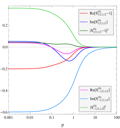
Figure 1: Dependence of $\text{Re}[S_{1/2,1/2}^{\left(0\right)}-1]$, $\text{Im}[S_{1/2,1/2}^{\left(0\right)}]$, $|S_{1/2,1/2}^{\left(0\right)}|^{2}$, $\text{Re}[S_{-1/2,1/2}^{\left(0\right)}]$, $\text{Im}[S_{-1/2,1/2}^{\left(0\right)}]$, and $|S_{-1/2,1/2}^{\left(0\right)}|^{2}$ on the fermion momentum $p$.

It was found that the $p$-dependences of the partial matrix elements $S_{I_{3}^{\prime},I_{3}}^{\left(0\right)}$, $S_{I_{3}^{\prime},I_{3}}^{\left(\pm 1\right)}$, and $S_{I_{3}^{\prime},I_{3}}^{\left(\left|m\right|\geq 2\right)}$ are substantially different, and we therefore consider them separately here. For better visualization of the $p$-dependences, we show them on log-linear plots. Figure 1 shows the $p$-dependences related to the partial matrix elements $S_{\pm 1/2,1/2}^{\left(0\right)}$. We can see that all of the curves in Fig. 1 are regular functions of the fermion momentum $p$. In particular, they all tend to nonzero limits as $p\rightarrow 0$, and $|S_{1/2,1/2}^{\left(0\right)}-1|^{2}$, $|S_{-1/2,1/2}^{\left(0\right)}|^{2}$, $|\text{Re}[S_{1/2,1/2}^{\left(0\right)}-1]|$, and $|\text{Im}[S_{-1/2,1/2}^{\left(0\right)}]|$ reach their maximal values at $p=0$.

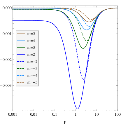
Figure 2: Dependence of $\text{Re}[S_{1/2,1/2}^{\left(m\right)}-1]$ on the fermion momentum $p$ for $|m|=2,3,4,\,\text{and}\;5$.

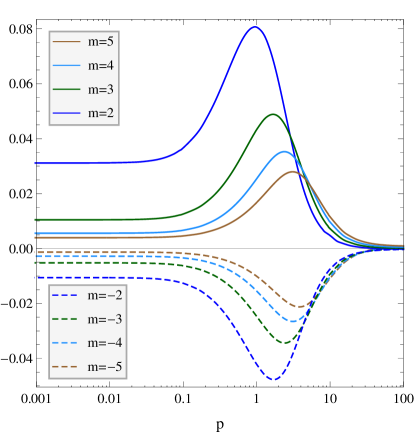
Figure 3: Dependence of $\text{Im}[S_{1/2,1/2}^{\left(m\right)}]$ on the fermion momentum $p$ for $|m|=2,3,4,\,\text{and}\;5$.

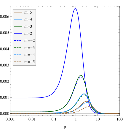
Figure 4: Dependence of $|S_{1/2,1/2}^{\left(m\right)}-1|^{2}$ on the fermion momentum $p$ for $|m|=2,3,4,\,\text{and}\;5$.

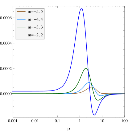
Figure 5: Dependence of $\text{Re}[S_{-1/2,1/2}^{\left(m\right)}]$ on the fermion momentum $p$ for $|m|=2,3,4,\,\text{and}\;5$.

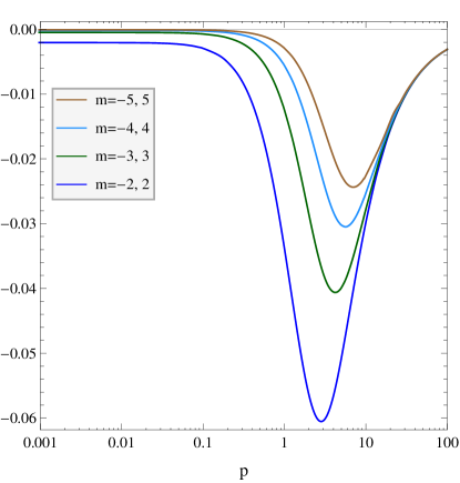
Figure 6: Dependence of $\text{Im}[S_{-1/2,1/2}^{\left(m\right)}]$ on the fermion momentum $p$ for $|m|=2,3,4,\,\text{and}\;5$.

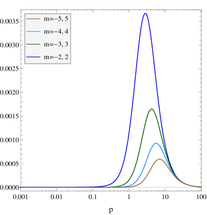
Figure 7: Dependence of $|S_{-1/2,1/2}^{\left(m\right)}|^{2}$ on the fermion momentum $p$ for $|m|=2,3,4,\,\text{and}\;5$.

Figures 2 – 7 show the real parts, imaginary parts, and squared magnitudes of the partial matrix elements $S_{\pm 1/2,1/2}^{\left(m\right)}$ as functions of the fermion momentum $p$. The $p$-dependences are shown for $\left|m\right|=2,3,4,\text{ and}\,5$. We can see that for $\left|m\right|\geq 2$, the curves of $\text{Re }[S_{1/2,1/2}^{\left(m\right)}\left(p\right)-1]$, $\text{Im}[S_{1/2,1/2}^{\left(m\right)}\left(p\right)]$, $|S_{1/2,1/2}^{\left(m\right)}\left(p\right)-1|^{2}$, $\text{Re}[S_{-1/2,1/2}^{\left(m\right)}\left(p\right)]$, $\text{Im}[S_{-1/2,1/2}^{\left(m\right)}\left(p\right)]$, and $|S_{-1/2,1/2}^{\left(m\right)}\left(p\right)|^{2}$ have similar forms. All of them have wide extrema at moderate values of $p$, and tend to zero as $p\rightarrow\infty$ and to constant values as $p\rightarrow 0$. The only difference is that for $\left|m\right|=2,3,\text{and}\,4$, the $\text{Re}[S_{-1/2,1/2}^{\left(m\right)}\left(p\right)]$ curves have a node located to the right of the maximum at moderate values of $p$.

It follows from Fig. 3 that the imaginary parts of the elastic partial elements of the $S$-matrix satisfy the approximate relation

$$\text{Im}[S_{1/2,1/2}^{\left(m\right)}(p)]\approx\text{Im}[S_{1/2,1/2}^{\left(-m+1\right)}(p)].$$ (66)

Since $|\text{Im}[S_{1/2,1/2}^{\left(m\right)}]|\gg|\text{Re}[S_{1/2,1/2}^{\left(m\right)}-1]|$, approximate equality (66) results in the approximate equality of the squared magnitudes $|S_{1/2,1/2}^{\left(m\right)}-1|^{2}\approx|S_{1/2,1/2}^{\left(-m+1\right)}-1|^{2}$, as shown in Fig. 4. It follows from Eqs. (17) and (18) that for $n=1$, the change $m\rightarrow-m+1$ of the grand spin $K_{3}$ leads only to the interchange of the absolute values of the orbital angular momenta $|l_{11}|$ and $|l_{21}|$. It follows from Eq. (26) that the centrifugal barrier does not change as a whole for the elastic channel of fermion scattering, and thus the fermion-soliton interaction is of the same order for the partial elastic channels with $K_{3}=m$ and $K_{3}=-m+1$. This may explain the close values of the dominant imaginary parts in Eq. (66).

We also found that the position of the maximum in $|S_{1/2,1/2}^{\left(m\right)}-1|^{2}$ is approximately determined by the linear expression

$$p_{\text{max}}\approx 0.64\left|m-1/2\right|,$$ (67)

whereas the heights of the maxima decrease monotonically (approximately $\propto\left|m\right|^{-2}$) with an increase in $\left|m\right|$. Note that Eq. (67) is compatible with Eq. (66) since $\left|m-1/2\right|$ is equal to $m-1/2$ for positive $m$ and $\left(-m+1\right)-1/2$ for negative $m$. Eq. (67) can be explained as follows. The partial matrix elements $S_{1/2,1/2}^{\left(m\right)}$ describe the elastic fermion scattering in the state with grand spin $K_{3}=m$. Eq. (15) tells us that with an increase in $\left|m\right|$, the main contribution to $K_{3}$ comes from the orbital part. Next, it follows from Eqs. (17) and (18) that for $n=1$, the orbital angular momenta of the elastic components $c_{11}$ and $c_{21}$ of the fermion radial wave function are $l_{11}=m-1$ and $l_{21}=m$, respectively. We see that both $l_{11}$ and $l_{21}$ depend linearly on $m$. In the classical limit, the absolute value of the orbital angular momentum $\left|l\right|=bp$, where $b$ is an impact parameter. In our case, the impact parameter $b$ should be on the order of the soliton’s size $r_{0}$. In the momentum representation, the fermion radial wave function $c_{ia}$ that corresponds to the state with $K_{3}=m$ should have a maximum in the neighborhood of the classical value $p=\left|l\right|/b$, in accordance with Eq. (67).

It follows from Figs. 5 – 7 that in accordance with Eq. (44), the inelastic partial matrix elements $S_{-1/2,1/2}^{\left(m\right)}$ coincide when they have opposite values of $m$. Furthermore, similarly to Eq. (67) and for the same reasons, the position of the maximum of $|S_{-1/2,1/2}^{\left(m\right)}|^{2}$ is also determined by the linear expression

$$p_{\text{max}}\approx 1.37\left|m\right|.$$ (68)

From a comparison between the $p$-dependences related to $S_{\pm 1/2,1/2}^{\left(0\right)}$ and those related to $S_{\pm 1/2,1/2}^{\left(|m|\geq 2\right)}$, we can see two main differences. Firstly, there are no pronounced maxima for $|S_{I_{3}^{\prime},I_{3}}^{\left(0\right)}-\delta_{I_{3}^{\prime},I_{3}}|^{2}$ at nonzero $p$, since for $m=0$, the contribution of the orbital part to the grand spin $K_{3}$ is not dominant in comparison with those of the spin and isospin parts. Secondly, the limiting values of $|S_{I_{3}^{\prime},I_{3}}^{\left(0\right)}-\delta_{I_{3}^{\prime},I_{3}}|^{2}$ are much greater than those of $|S_{I_{3}^{\prime},I_{3}}^{\left(\left|m\right|>2\right)}-\delta_{I_{3}^{\prime},I_{3}}|^{2}$ as $p\rightarrow 0$. This is because according to Eq. (18), both $l_{21}$ and $l_{12}$ vanish when $m=0$ and $n=1$. It follows that in this case, the centrifugal barrier is absent for both elastic and inelastic fermion scattering. This leads to intense interactions between the fermions and the core of the soliton. In turn, this results in large squared magnitudes for both the elastic and inelastic partial elements of the $S$-matrix.

Using numerical methods, we were also able to ascertain some other features of the curves shown in Figs. 1 – 7. In particular, we ascertained the asymptotic behavior of $S_{I_{3}^{\prime},I_{3}}^{\left(m\right)}(p)$ as $p\rightarrow\infty$:

$$\text{Re}\left[S_{1/2,1/2}^{\left(m\right)}-1\right] \sim \alpha\left(m\right)p^{-2},$$ (69a)

$$\text{Im}\left[S_{1/2,1/2}^{\left(m\right)}\right] \sim \beta\left(m\right)p^{-1},$$ (69b)

$$\text{Re}\left[S_{-1/2,1/2}^{\left(m\right)}\right] \sim \gamma\left(m\right)p^{-1},$$ (69c)

$$\text{Im}\left[S_{-1/2,1/2}^{\left(m\right)}\right] \sim -\pi hp^{-1},$$ (69d)

where $\alpha\left(m\right)$, $\beta\left(m\right)$, and $\gamma\left(m\right)$ are $m$-dependent constants. Note that for $\text{Im}[S_{-1/2,1/2}^{\left(m\right)}]$, we were able to find the exact form of the coefficient of the leading asymptotic term. This is because the Born approximation (58) perfectly describes the behavior of $\text{Im}[S_{-1/2,1/2}^{\left(m\right)}]$ for $p\gtrsim 10$. At the same time, the Born approximation (58) gives only a qualitative description of $\text{Im}[S_{1/2,1/2}^{\left(m\right)}]$: it gives the correct ($\propto p^{-1}$) leading asymptotic behavior, but an incorrect factor before the leading asymptotic term. Note that in Eq. (69a), the leading asymptotic term is $\propto p^{-2}$, while in Eqs. (69b) – (69d), the leading asymptotic terms are $\propto p^{-1}$. This difference is due to the fact that $\text{Im}[S_{1/2,1/2}^{\left(m\right)}]$, $\text{Re}[S_{-1/2,1/2}^{\left(m\right)}]$, and $\text{Im}[S_{-1/2,1/2}^{\left(m\right)}]$ tend to zero as $p\rightarrow\infty$, while $\text{Re}[S_{1/2,1/2}^{\left(m\right)}]$ tends to one in this limit. It can then easily be shown that asymptotic behavior (69a) follows from the fulfillment of the unitarity condition $|S_{1/2,1/2}^{\left(m\right)}|^{2}+|S_{-1/2,1/2}^{\left(m\right)}|^{2}=1$ in the leading order in inverse powers of $p$.

It follows from Figs. 1 – 7 that as $p$ tends to zero, the real and imaginary parts of the difference $S_{I_{3}^{\prime},I_{3}}^{\left(m\right)}-\delta_{I_{3}^{\prime},I_{3}}$ tend to some constants whose absolute values decrease monotonically with an increase in $\left|m\right|$. Then, Eqs. (33) and (37) tell us that both the elastic and inelastic partial cross-sections $\sigma_{I_{3}^{\prime},I_{3}}^{\left(m\right)}=p^{-1}|S_{I_{3}^{\prime},I_{3}}^{\left(m\right)}-\delta_{I_{3}^{\prime},I_{3}}|^{2}$ diverge as $p^{-1}$ when $p\rightarrow 0$.

Next we turn to the partial matrix elements $S_{\pm 1/2,1/2}^{\left(\pm 1\right)}$. The dependence of the real and imaginary parts of $S_{\pm 1/2,1/2}^{\left(+1\right)}$ on the fermion momentum $p$ is shown in Fig. 8. We can see that the $p$-dependences in Fig. 8 are in sharp contrast to those in Figs. 1 – 7. In particular, the $p$-dependence of the elastic partial element $S_{1/2,1/2}^{\left(+1\right)}$ shows pronounced resonance behavior at extremely low values of $p$. We were able to achieve extremely small values of $p$ to reveal two resonance valleys of $\text{Re}[S_{1/2,1/2}^{\left(+1\right)}]$. The positions of the extrema in $\text{Re}[S_{1/2,1/2}^{\left(+1\right)}]$ coincide with those of the zeros of $\text{Im}[S_{1/2,1/2}^{\left(+1\right)}]$, as expected for resonance structures. Note that $\text{Re}[S_{1/2,1/2}^{\left(+1\right)}]$ (and hence $|S_{1/2,1/2}^{\left(+1\right)}|$) reaches the unitary boundary of $1$ at its maxima. Hence, the elastic partial cross-section $\sigma_{1/2,1/2}^{(+1)}$ vanishes at the maxima of $\text{Re}[S_{1/2,1/2}^{\left(+1\right)}]$ as well as the inelastic partial cross-section $\sigma_{-1/2,1/2}^{(+1)}$. Note that both $\text{Re}[S_{1/2,1/2}^{\left(+1\right)}]$ and $\text{Im}[S_{1/2,1/2}^{\left(+1\right)}]$ do not reach the unitary boundary of $-1$ at their minima, although these are in close proximity. This follows from the fact that the inelastic scattering does not vanish at the minima of $\text{Re}[S_{1/2,1/2}^{\left(+1\right)}]$ and $\text{Im}[S_{1/2,1/2}^{\left(+1\right)}]$. For a similar reason, $\text{Im}[S_{1/2,1/2}^{\left(+1\right)}]$ also does not quite reach the unitary boundary of $1$ at its maxima.

The $p$-dependences of the real and imaginary parts of the inelastic partial matrix element $S_{-1/2,1/2}^{\left(+1\right)}$ also have a resonance structure at small values of $p$. Moreover, the positions of the minima (maxima) of $\text{Re}[S_{-1/2,1/2}^{\left(+1\right)}]$ coincide with those of the maxima (minima) of $\text{Re}[S_{1/2,1/2}^{\left(+1\right)}]$, and a similar situation holds for the imaginary parts $\text{Im}[S_{-1/2,1/2}^{\left(+1\right)}]$ and $\text{Im}[S_{1/2,1/2}^{\left(+1\right)}]$. The positions of the zeros of $\text{Re}[S_{-1/2,1/2}^{\left(+1\right)}]$, $\text{Im}[S_{-1/2,1/2}^{\left(+1\right)}]$, and $\text{Im}[S_{1/2,1/2}^{\left(+1\right)}]$ also coincide, since $\text{Re}[S_{1/2,1/2}^{\left(+1\right)}]$ reaches the unitary boundary of $1$ at this point. Note that in Fig. 8, the behavior of the curves is in accordance with the unitarity condition $|S_{1/2,1/2}^{\left(+1\right)}|^{2}+|S_{-1/2,1/2}^{\left(+1\right)}|^{2}=1$.

Figure 9 presents the $p$-dependence of the real and imaginary parts of the partial matrix elements $S_{\pm 1/2,1/2}^{\left(-1\right)}$. We see that in accordance with Eq. (44), the curves of $\text{Re}[S_{-1/2,1/2}^{\left(-1\right)}]$ and $\text{Im}[S_{-1/2,1/2}^{\left(-1\right)}]$ coincide with the curves for $\text{Re}[S_{-1/2,1/2}^{\left(+1\right)}]$ and $\text{Im}[S_{-1/2,1/2}^{\left(+1\right)}]$ shown in Fig. 8. In particular, the curves of $\text{Re}[S_{-1/2,1/2}^{\left(-1\right)}]$ and $\text{Im}[S_{-1/2,1/2}^{\left(-1\right)}]$ have the same resonance structure as those of $\text{Re}[S_{-1/2,1/2}^{\left(+1\right)}]$ and $\text{Im}[S_{-1/2,1/2}^{\left(+1\right)}]$, respectively. In Fig. 9, the curves that correspond to the real and imaginary parts of the elastic partial matrix element $S_{1/2,1/2}^{\left(-1\right)}$ also show resonance-like behavior. However, the behavior of these curves differs from those of the other resonance curves in Figs. 8 and 9. In particular, the points of the maxima in $|S_{1/2,1/2}^{\left(-1\right)}|^{2}$ and $\text{Re}[S_{1/2,1/2}^{\left(-1\right)}]$ do not coincide, and $\text{Im}[S_{1/2,1/2}^{\left(-1\right)}]$ does not vanish at these points. Hence, it can be said that $S_{1/2,1/2}^{\left(-1\right)}$ does not show true resonance behavior. Instead, the resonance-like behavior of $S_{1/2,1/2}^{\left(-1\right)}$ is caused by the unitarity condition $|S_{1/2,1/2}^{\left(-1\right)}|^{2}+|S_{-1/2,1/2}^{\left(-1\right)}|^{2}=1$ and the true resonance behavior of the inelastic partial element $S_{-1/2,1/2}^{\left(-1\right)}$ of the $S$-matrix.

In Figs. 8 and 9, all $p$-dependencies are shown on a logarithmic scale. We see that in the resonance region, the $p$-dependences of $|S_{\pm 1/2,1/2}^{\left(\pm 1\right)}-\delta_{\pm 1/2,1/2}|^{2}$, $\text{Re}[S_{\pm 1/2,1/2}^{\left(\pm 1\right)}-\delta_{\pm 1/2,1/2}]$, and $\text{Im}[S_{\pm 1/2,1/2}^{\left(\pm 1\right)}]$ have the Breit-Wigner form on this scale. Also, the positions of resonance peaks are at extremely low values of the fermion momenta. Another feature is a periodic structure of the resonances in Figs. 8 and 9. In particular, the distance between the resonance peaks is approximately the same on the logarithmic scale. We were able to identify the two resonance peaks of $|S_{\pm 1/2,1/2}^{\left(\pm 1\right)}-\delta_{\pm 1/2,1/2}|^{2}$ and reach the beginning of the third one. Therefore, we may suppose the existence of a sequence of resonances (possibly infinite) condensing to the zero fermion momentum.

VI Conclusion

In the present paper, fermion scattering in the background fields of the topological solitons of the nonlinear $O(3)$ $\sigma$-model has been investigated both analytically and numerically. In particular, we have ascertained the asymptotic behavior of the fermion wave functions for both large and small values of the radial variable $r$. The symmetry properties of the partial elements of the $S$-matrix under discrete transformations of the Dirac Hamiltonian have been determined. In the framework of the first Born approximation, a complete analytical investigation of fermion scattering in the background field of the elementary topological soliton with winding number $n=1$ has been carried out. In particular, the Born amplitudes, differential cross-sections, and total cross-sections of fermion scattering have been obtained in analytical form. The asymptotic behavior of the partial Born amplitudes has been investigated for extreme values of the fermion momentum, momentum transfer, and grand spin.

We have also performed a numerical study of fermion scattering in the background field of the elementary topological solition of the nonlinear $O(3)$ $\sigma$-model. In particular, we have obtained the $p$-dependences of the partial elements $S_{I_{3}^{\prime},I_{3}}^{\left(m\right)}$ of the $S$-matrix for $\left|m\right|\leq 5$, and have ascertained their main features. In particular, we found that the partial elements $S_{I_{3}^{\prime},I_{3}}^{\left(\pm 1\right)}$ of the $S$-matrix show resonance behavior at small values of the fermion momentum.

Appendix A Free fermions

Let the isovector scalar field $\bm{\phi}$ be a constant field that takes the value $(0,0,-1)$. This situation corresponds to the vacuum state in the topologically trivial sector $(n=0)$ or distant regions in the topologically nontrivial sectors $(n\neq 0)$. In this case, the Dirac equation (6) is written as

$$i\gamma^{\mu}\otimes\mathbb{I}\partial_{\mu}\psi-h\mathbb{I}\otimes\tau_{3}\psi=0$$ (70)

or in the Hamiltonian form:

$$i\frac{\partial\psi}{\partial t}=H_{0}\psi,$$ (71)

where the free Hamiltonian

$$H_{0}=\alpha^{k}\otimes\mathbb{I}\left(-i\partial_{k}\right)+h\beta\otimes\tau_{3}.$$ (72)

The Dirac equation (70) is invariant under the $C$, $P$ and $\Pi_{2}T$ transformations:

$$\psi\left(t,\mathbf{x}\right) \rightarrow \psi^{C}\left(t,\mathbf{x}\right)=i\gamma^{1}\mathbb{\otimes I\,}\psi^{\ast}\left(t,\mathbf{x}\right),$$ (73)

$$\psi\left(t,\mathbf{x}\right) \rightarrow \psi^{P}\left(t,\mathbf{x}\right)=\gamma^{0}\mathbb{\otimes I}\psi\left(t,-\mathbf{x}\right),$$ (74)

$$\psi\left(t,\mathbf{x}\right) \rightarrow \psi^{\Pi_{2}T}\left(t,\mathbf{x}\right)=\psi^{\ast}\left(-t,x_{1},-x_{2}\right).$$ (75)

The Hamiltonian (72) commutes with the operator of grand spin (15), which is reduced to the operator of the usual angular momentum in the topologically trivial background vacuum field $\bm{\phi}_{\text{ vac}}=(0,0,-1)$. It also commutes with the isospin generator $I_{3}=\tau_{3}/2$ and the momentum operator $\mathbf{\hat{p}}=-i\nabla$. It therefore follows that the free fermionic states can be characterized either by the momentum $\mathbf{p}$ and the third isospin component $I_{3}$ (plane waves) or by the grand spin $K_{3}$ and the third isospin component $I_{3}$ (cylindrical waves).

In the compact matrix form, the plane-wave fermionic states $\psi_{\pm p,I_{3}}$ with positive and negative energies can be written as

$$\psi_{p,1/2}=\frac{1}{\sqrt{2\varepsilon}}\begin{pmatrix}\sqrt{\varepsilon+h}&0\\ i\sqrt{\varepsilon-h}e^{i\theta_{\mathbf{p}}}&0\end{pmatrix}e^{-ipx},$$ (76a)

$$\psi_{p,-1/2}=\frac{1}{\sqrt{2\varepsilon}}\begin{pmatrix}0&-i\sqrt{\varepsilon-h}e^{-i\theta_{\mathbf{p}}}\\ 0&\sqrt{\varepsilon+h}\end{pmatrix}e^{-ipx},$$ (76b)

$$\psi_{-p,1/2}=\frac{1}{\sqrt{2\varepsilon}}\begin{pmatrix}-i\sqrt{\varepsilon-h}e^{-i\theta_{\mathbf{p}}}&0\\ \sqrt{\varepsilon+h}&0\end{pmatrix}e^{ipx},$$ (76c)

$$\psi_{-p,-1/2}=\frac{1}{\sqrt{2\varepsilon}}\begin{pmatrix}0&\sqrt{\varepsilon+h}\\ 0&i\sqrt{\varepsilon-h}e^{i\theta_{\mathbf{p}}}\end{pmatrix}e^{ipx},$$ (76d)

where $p=\left(\varepsilon,\mathbf{p}\right)$, $px=\varepsilon t-\mathbf{p}\!\bm{\cdot}\!\mathbf{x}$, and $\theta_{\mathbf{p}}$ is the azimuthal angle of the momentum $\mathbf{p}$. Note that the negative energy wave functions are $C$-conjugates of the positive energy wave functions, $\psi_{-p,\,I_{3}}=\left(\psi_{p,\,I_{3}}\right)^{C}=\sigma_{1}\mathbb{\otimes I\,}\psi_{p,\,I_{3}}^{\ast}$. The wave functions $\psi_{\pm p,I_{3}}$ and their amplitudes $u_{\pm p,I_{3}}$ defined by the formula $\psi_{\pm p,I_{3}}=\left(2\varepsilon\right)^{-1/2}u_{\pm p,I_{3}}e^{\mp ipx}$ satisfy the normalization conditions:

$$\bar{\psi}_{\pm p,\,I_{3}}\gamma^{\mu}\otimes\mathbb{I}\psi_{\pm p,\,I_{3}}=\left(1,\frac{p_{x}}{\varepsilon},\frac{p_{y}}{\varepsilon}\right)=\left(1,\,\mathbf{v}\right)$$ (77)

and

$$\bar{u}_{\pm p,I_{3}^{\prime}}u_{\pm p,\,I_{3}}=(-1)^{1/2\mp I_{3}}2h\delta_{I_{3}^{\prime},I_{3}},\quad\bar{u}_{p,I_{3}^{\prime}}u_{-p,\,I_{3}}=0.$$ (78)

It follows that the wave functions $\psi_{\pm p,I_{3}}$ have the normalization

$$\int\bar{\psi}_{\pm p^{\prime},I_{3}^{\prime}}(\mathbf{x})\psi_{\pm p,I_{3}}(\mathbf{x})d^{2}\mathbf{x}= (-1)^{1/2\mp I_{3}}\frac{h}{\varepsilon}\left(2\pi\right)^{2}$$

$$\times\delta_{I_{3}^{\prime},I_{3}}\delta^{\left(2\right)}\left(\mathbf{p}-\mathbf{p}^{\prime}\right),$$ (79)

where it is understood that in Eqs. (77)–(79), the summation is performed over the spin and isospin indices of the corresponding wave functions and amplitudes.

Let us consider the cylinder-wave fermionic states $\psi_{p,m,I_{3}}$ that possess definite values of the grand spin $K_{3}$ and the isospin $I_{3}$. For free fermions, the matrix $\Lambda$ in Eq. (24) takes the form

$$\Lambda_{ia;jb}=\left(\begin{array}[]{cccc}\dfrac{l_{11}}{r}&0&\varepsilon+h&0\\ 0&\dfrac{l_{12}}{r}&0&\varepsilon-h\\ -\varepsilon+h&0&-\dfrac{l_{21}}{r}&0\\ 0&-\varepsilon-h&0&-\dfrac{l_{22}}{r}\end{array}\right),$$ (80)

where the orbital quantum numbers $l_{ia}$ are defined in Eq. (18). We see that system (24) can be split into two independent subsystems that correspond to the two isospin states $\pm 1/2$. These two subsystems can be solved analytically, and their positive energy regular solutions are

$$\psi_{p,m,1/2} =\begin{pmatrix}\sqrt{\frac{p\left(\varepsilon+h\right)}{2\varepsilon}}J_{l_{11}}\left(pr\right)e^{il_{11}\theta}&0\\ -\sqrt{\frac{p\left(\varepsilon-h\right)}{2\varepsilon}}J_{l_{21}}\left(pr\right)e^{il_{21}\theta}&0\end{pmatrix}e^{-i\varepsilon t}\sim\sqrt{\frac{2}{\pi r}}\begin{pmatrix}\sqrt{\frac{\varepsilon+h}{2\varepsilon}}\sin\left[pr-\pi\left(2l_{11}-1\right)/4\right]e^{il_{11}\theta}&0\\ \sqrt{\frac{\varepsilon-h}{2\varepsilon}}\sin\left[pr-\pi\left(2l_{21}+3\right)/4\right]e^{il_{21}\theta}&0\end{pmatrix}e^{-i\varepsilon t},$$ (81a)

$$\psi_{p,m,-1/2} =\begin{pmatrix}0&-\sqrt{\frac{p\left(\varepsilon-h\right)}{2\varepsilon}}J_{l_{12}}\left(pr\right)e^{il_{12}\theta}\\ 0&\sqrt{\frac{p\left(\varepsilon+h\right)}{2\varepsilon}}J_{l_{22}}\left(pr\right)e^{il_{22}\theta}\end{pmatrix}e^{-i\varepsilon t}\sim\sqrt{\frac{2}{\pi r}}\begin{pmatrix}0&\sqrt{\frac{\varepsilon-h}{2\varepsilon}}\sin\left[pr-\pi\left(2l_{12}+3\right)/4\right]e^{il_{12}\theta}\\ 0&\sqrt{\frac{\varepsilon+h}{2\varepsilon}}\sin\left[pr-\pi\left(2l_{22}-1\right)/4\right]e^{il_{22}\theta}\end{pmatrix}e^{-i\varepsilon t},$$ (81b)

where $p=\left|\bf{p}\right|$ and $J_{\nu}(pr)$ are the Bessel functions of the first kind. The negative energy regular solutions are obtained from Eqs. (81) by means of $C$-conjugation (73). Wave functions (81) satisfy the normalization condition

$$\int\psi_{p^{\prime},m^{\prime},I_{3}^{\prime}}^{\ast}(r,\theta)\psi_{p,m,I_{3}}(r,\theta)rdrd\theta= 2\pi\delta_{m^{\prime}\!,m}\delta_{I_{3}^{\prime},I_{3}}$$

$$\times\delta\left(p\!-\!p^{\prime}\right)\!.$$ (82)

Unlike wave functions (76), wave functions (81) have definite parity under $P$-transformation (74)

$$\psi^{P}_{p,m,I_{3}}\left(t,\mathbf{x}\right) =\gamma^{0}\!\otimes\!\mathbb{I}\psi_{p,m,I_{3}}\left(t,-\mathbf{x}\right)$$

$$=\left(-1\right)^{m-nI_{3}-\frac{1}{2}}\psi_{p,m,I_{3}}\left(t,\mathbf{x}\right)\!$$ (83)

and are invariant under $\Pi_{2}T$-transformation (75).

The plane-wave fermionic states $\psi_{p,I_{3}}$ can be expanded in terms of the cylinder-wave fermionic states $\psi_{p,m,I_{3}}$. To do this, we use the well-known expansion of the plane wave in terms of cylinder waves

$$e^{ipx}=e^{ipr\cos\left(\theta\right)}=\sum_{i=-\infty}^{\infty}i^{m}J_{m}\left(pr\right)e^{im\theta}.$$ (84)

Eqs. (76), (81), and (84) give us the expansion

$$\psi_{\left(\varepsilon,p,0\right),\,I_{3}}=\sum_{m=-\infty}^{\infty}a_{p,m,I_{3}}\psi_{p,m,I_{3}},$$ (85)

where the expansion coefficients

$$a_{p,m,I_{3}}=i^{m-I_{3}\left(n+1\right)}p^{-1/2}$$ (86)

and all components of the $(2+1)$-dimensional momentum of the plane-wave state are explicitly shown on the left-hand side of Eq. (85). Note that Eq. (86) is valid only for the positive energy fermionic states. To obtain the expansion coefficients for the negative energy fermionic states, we must take the complex conjugate of the right-hand side of Eq. (86).

Appendix B Resonances of partial amplitudes at small fermion momenta

Let us ascertain the cause of occurrence of the resonance peaks in the partial channel with grand spin $m=1$. It follows from Eqs. (18), (26), and (34) that the characteristic feature of this partial channel is the absence of both the kinematic suppression factor $(\varepsilon-h)^{1/2}$ and the centrifugal barrier for the $c_{11}$ component of the radial wave function $c_{ia}(r)$. As a result, the $c_{11}$ component is much larger than the other three components of $c_{ia}(r)$. Using this fact, we can find an approximate solution to system (24) for small values of $p$. To do this, we perform two iterations. At the first iteration, we suppose that $c_{11}(r)$ is a constant $\alpha_{0}$ and find $c_{12}(r)$, $c_{21}(r)$, and $c_{22}(r)$ neglecting all terms except centrifugal and those that proportional to $\alpha_{0}$. At the second iteration, we substitute $c_{12}(r)$, $c_{21}(r)$, and $c_{22}(r)$ into the differential equation for $c_{11}(r)$ and integrate this equation. As a result, we obtain the approximate iterative solution for the radial wave function $c_{ia}(r)$

$$c_{11}\left(r\right) = \frac{\alpha_{0}}{12}\Bigl{\{}12-3p^{2}r^{2}-hr_{0}^{2}\left(\varepsilon+h\right)\Bigr{.}$$ (87a)

$$\times\Bigl{(}\pi^{2}-3\ln\left[\left(r^{2}+r_{0}^{2}\right)r_{0}^{-2}\right]\Bigr{.}$$

$$\times\left.\left(2+\ln\left[r_{0}^{2}\left(r^{2}+r_{0}^{2}\right)r^{-4}\right]\right)\right.$$

$$\left.\left.-6\text{Li}_{2}\left[r_{0}^{2}\left(r^{2}+r_{0}^{2}\right)^{-1}\right]\right)\right\},$$

$$c_{12}\left(r\right) = \beta_{0}r-2^{-1}\alpha_{0}hr_{0}^{3}\left(\varepsilon+h\right)r^{-1}$$ (87b)

$$\times\ln\left[\left(r^{2}+r_{0}^{2}\right)r_{0}^{-2}\right],$$

$$c_{21}\left(r\right) = -2^{-1}\alpha_{0}\left(\varepsilon-h\right)r-\alpha_{0}hr_{0}^{2}r^{-1}$$ (87c)

$$\times\ln\left[\left(r^{2}+r_{0}^{2}\right)r_{0}^{-2}\right],$$

$$c_{22}\left(r\right) = \alpha_{0}hr_{0}\left(r_{0}^{2}r^{-2}\ln\left[\left(r^{2}\!+\!r_{0}^{2}\right)r_{0}^{-2}\right]\!-\!1\right),$$ (87d)

where $\alpha_{0}$ and $\beta_{0}$ are constants, and $\text{Li}_{2}$ is the dilogarithm function.

At small $r$, the components of the radial wave function can be written as

$$c_{11}\left(r\right) = \alpha_{0}-2^{-2}\alpha_{0}p^{2}r^{2}+O\left(r^{4}\right),$$ (88a)

$$c_{12}\left(r\right) = \left(\beta_{0}-2^{-1}\alpha_{0}hr_{0}\left(\varepsilon+h\right)\right)r$$ (88b)

$$+O\left(r^{3}\right)\!,$$

$$c_{21}\left(r\right) = -2^{-1}\alpha_{0}\left(\varepsilon+h\right)r+O\left(r^{3}\right),$$ (88c)

$$c_{22}\left(r\right) = -2^{-1}\alpha_{0}hr_{0}^{-1}r^{2}+O\left(r^{4}\right)$$ (88d)

in accordance with Eq. (26). It was found that in a wide area of $r$, the components of the radial wave function satisfy the conditions

$$\left|c_{11}\right| \gtrsim \alpha_{0}\left(1-13.6\tau^{2}\right),$$ (89a)

$$\left|c_{12}\right| \lesssim 0.8\alpha_{0}\tau^{2},$$ (89b)

$$\left|c_{21}\right| \lesssim 0.8\alpha_{0}\tau,$$ (89c)

$$\left|c_{22}\right| \lesssim \alpha_{0}\tau,$$ (89d)

where the parameter $\tau=hr_{0}$. We see that under the condition $\tau\ll 1$, the absolute value of the $c_{11}$ component is much larger than those of the other three components of the radial wave function.

When the distance from the core of the soliton is sufficiently large, we can neglect the fermion-soliton interaction. In this case, the general solution to system (24) is written as

$$c_{11}\left(r\right) \sim C_{1}J_{0}\left(pr\right)+C_{2}Y_{0}\left(pr\right),$$ (90a)

$$c_{12}\left(r\right) \sim -\sqrt{\frac{\varepsilon-h}{\varepsilon+h}}\left(C_{3}J_{1}\left(pr\right)+C_{4}Y_{1}\left(pr\right)\right),$$ (90b)

$$c_{21}\left(r\right) \sim -\sqrt{\frac{\varepsilon-h}{\varepsilon+h}}\left(C_{1}J_{1}\left(pr\right)+C_{2}Y_{1}\left(pr\right)\right),$$ (90c)

$$c_{22}\left(r\right) \sim C_{3}J_{2}\left(pr\right)+C_{4}Y_{2}\left(pr\right),$$ (90d)

where $C_{1}$ – $C_{4}$ are constant coefficients, $J_{\nu}$ and $Y_{\nu}$ are the Bessel and Neumann functions of corresponding orders, respectively. Using standard methods from the theory of scattering [32, 33], we obtain the expressions for the partial elements of the $S$-matrix in terms of the coefficients $C_{1}$ – $C_{4}$

$$S_{1/2,1/2}^{\left(+1\right)} = \frac{C_{1}-iC_{2}}{C_{1}+iC_{2}},$$ (91a)

$$S_{-1/2,1/2}^{\left(+1\right)} = \frac{2p}{\varepsilon-h}\frac{C_{3}}{C_{1}+iC_{2}}.$$ (91b)

To express the coefficients $C_{1}$ – $C_{4}$ in terms of physical parameters, we join solutions (87) and (90) at $r=\kappa r_{0}$, where $\kappa$ is a positive coefficient greater than one. The resulting expressions for $C_{1}$ – $C_{4}$ are too lengthy to be presented here. Expanding these expressions in $p$, holding lower-order terms, and substituting the resulting expressions in Eq. (91), we obtain the partial matrix elements:

$$S_{1/2,1/2}^{\left(+1\right)}=\frac{A+\pi^{-1}\Gamma\ln\left[pr_{0}\right]+i\Gamma/2}{A+\pi^{-1}\Gamma\ln\left[pr_{0}\right]-i\Gamma/2},$$ (92)

and

$$S_{-1/2,1/2}^{\left(+1\right)}=\frac{-i\tau\Gamma}{A+\pi^{-1}\Gamma\ln\left[pr_{0}\right]-i\Gamma/2}$$ (93)

where

$$A = 1+\kappa^{2}-\frac{1}{6}\tau^{2}\left(\left(12\gamma+\pi^{2}\right)\kappa^{2}+\pi^{2}\right)$$

$$+\frac{1}{2}\tau^{2}\left\{2\kappa^{2}\ln\left[4\left(\kappa^{2}+1\right)\kappa^{-2}\right]\right.$$

$$\left.+\left\{4\left(\kappa^{2}+1\right)\left(\gamma+\ln\left[2^{-1}\left(\kappa^{2}+1\right)^{1/4}\right]\right)+2\right\}\right.$$

$$\times\left.\ln\left[\kappa^{2}+1\right]\right\}+\tau^{2}\left(\kappa^{2}+1\right)\text{Li}_{2}\left[\left(\kappa^{2}+1\right)^{-1}\right],$$

$$\Gamma=2\pi\tau^{2}\left(\left(\kappa^{2}+1\right)\ln\left[\kappa^{2}+1\right]-\kappa^{2}\right),$$ (95)

and $\gamma$ is the Euler-Mascheroni constant.

Using Eqs. (92), (93), and (33), we obtain the expressions for the squared magnitudes of the partial amplitudes $f_{1/2,1/2}^{\left(+1\right)}$ and $f_{-1/2,1/2}^{\left(+1\right)}$:

$$\left|f_{1/2,1/2}^{\left(+1\right)}\right|^{2}=\frac{2}{\pi p}\frac{\left(\Gamma/2\right)^{2}}{\left(A+\pi^{-1}\Gamma\ln\left[pr_{0}\right]\right)^{2}+\left(\Gamma/2\right)^{2}},$$ (96)

and

$$\left|f_{-1/2,1/2}^{\left(+1\right)}\right|^{2}=\frac{1}{2\pi p}\frac{\Gamma_{r}\Gamma}{\left(A+\pi^{-1}\Gamma\ln\left[pr_{0}\right]\right)^{2}+\left(\Gamma/2\right)^{2}},$$ (97)

where

$$\Gamma_{r}=\tau^{2}\Gamma.$$ (98)

We can see that the squared magnitudes of the partial amplitudes $f_{1/2,1/2}^{\left(+1\right)}$ and $f_{-1/2,1/2}^{\left(+1\right)}$, considered as functions of the logarithmic variable $\pi^{-1}\Gamma\ln\left[pr_{0}\right]$, show resonance behavior of the Breit-Wigner type with total decay width equal to $\Gamma$. It follows that on the logarithmic scale, the squared magnitudes $|S_{I_{3}^{\prime},I_{3}}^{\left(+1\right)}-\delta_{I_{3}^{\prime},I_{3}}|^{2}=2\pi p|f_{I_{3}^{\prime},I_{3}}^{\left(+1\right)}|^{2}$ are of the symmetric Breit-Wigner form in the resonance region, as it is in Fig. 8. At the same time, the resonance peaks of $|S_{I_{3}^{\prime},I_{3}}^{\left(+1\right)}-\delta_{I_{3}^{\prime},I_{3}}|^{2}$ have a strongly asymmetric form in the linear scale. In particular, the resonance peaks have maxima at $p_{\max}=r_{0}^{-1}\exp\left(-\pi A/\Gamma\right)$ and reach half of the maxima at $p_{\pm 1/2}=r_{0}^{-1}\exp\left(-\pi A/\Gamma\pm\pi/2\right)$. The asymmetry of the resonance peaks is reflected in the relations

$$\frac{p_{+1/2}}{p_{\max}}=\frac{p_{\max}}{p_{-1/2}}=\exp\left(\pi/2\right)\approx 4.81048,$$ (99a)

and

$$\frac{p_{\max}-p_{-1/2}}{p_{+1/2}-p_{\max}}=\exp\left(-\pi/2\right)\approx 0.20788.$$ (99b)

The position of the maxima of the resonance peaks depends exponentially on the ratio $A/\Gamma$, which, in turn, depends on the parameters $\tau$ and $\kappa$. This results in extremely low values of $p_{\max}$ when $\tau\lesssim 0.1$ and $1\lesssim\kappa\lesssim 10^{2}$ in accordance with Figs. 8 and 9.

The existence of the resonance peaks and their logarithmic character are due to the term $\ln\left[pr_{0}\right]$ in Eqs. (92) and (93). In turn, this term results from the leading term of the expansion of the Neumann function $Y_{0}(pr)$ in the neighborhood of zero: $Y_{0}\left(pr\right)=2\pi^{-1}\left(\gamma-\ln\left(2\right)+\ln\left[pr\right]\right)+O(\left(pr\right)^{2}\ln\left[pr\right])$. Only the Neumann function $Y_{0}(pr)$ has the leading asymptotic behavior $\propto\ln[pr]$ as $pr\rightarrow 0$, whereas the other Neumann functions $Y_{l>0}(pr)\propto\left(pr\right)^{-l}$ in this limit. Therefore, the Neumann functions $Y_{l>0}(pr)$ cannot lead to resonance peaks of the logarithmic type.

It follows from Eq. (92) that the squared magnitude of $S_{1/2,1/2}^{\left(+1\right)}$ is equal to one. Therefore, the unitarity condition $|S_{1/2,1/2}^{\left(+1\right)}|^{2}+|S_{-1/2,1/2}^{\left(+1\right)}|^{2}=1$ is not satisfied in the used approach. Eq. (93) tells us that the squared magnitude of $S_{-1/2,1/2}^{\left(+1\right)}$ does not exceed the value of $4\tau^{2}=\left(2hr_{0}\right)^{2}$, which is equal to $0.04$ for the values of $h$ and $r_{0}$ used in Sec. V. It follows that the violation of the unitarity is small when the parameter $\tau=hr_{0}$ is much smaller than one.

The partial matrix elements (92) and (93) have a simple pole located at $p_{\text{pol}}=ir_{0}^{-1}\exp\left(-\pi A/\Gamma\right)=ip_{\max}$. According to the theory of scattering [32, 33], a pole of an elastic partial element of the $S$-matrix located at a positive imaginary momentum corresponds to a bound state. In our case, however, the presence of the pole is only an artifact of the used approach. Indeed, this pole exists for arbitrary small values of $h$ and $r_{0}$, which is impossible for bound states. We also failed to find fermion bound states in the partial channels with $m=\pm 1$ using numerical methods.

The obvious drawback of the used approach is that it is unable to explain the periodic structure of the resonance peaks in Figs. 8 and 9. This approach, however, can explain the location of the resonance peaks at extremely low fermion momenta and the Breit-Wigner form of these peaks on the logarithmic scale.

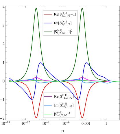
Figure 8: Dependence of $\text{Re}[S_{1/2,1/2}^{\left(+1\right)}-1]$, $\text{Im}[S_{1/2,1/2}^{\left(+1\right)}]$, $|S_{1/2,1/2}^{\left(+1\right)}|^{2}$, $\text{Re}[S_{-1/2,1/2}^{\left(+1\right)}]$, $\text{Im}[S_{-1/2,1/2}^{\left(+1\right)}]$, and $|S_{-1/2,1/2}^{\left(+1\right)}|^{2}$ on the fermion momentum $p$.

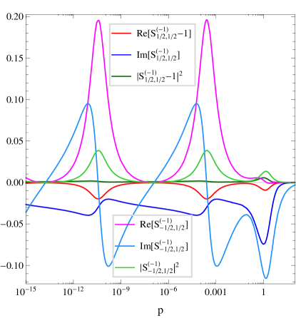
Figure 9: Dependence of $\text{Re}[S_{1/2,1/2}^{\left(-1\right)}-1]$, $\text{Im}[S_{1/2,1/2}^{\left(-1\right)}]$, $|S_{1/2,1/2}^{\left(-1\right)}|^{2}$, $\text{Re}[S_{-1/2,1/2}^{\left(-1\right)}]$, $\text{Im}[S_{-1/2,1/2}^{\left(-1\right)}]$, and $|S_{-1/2,1/2}^{\left(-1\right)}|^{2}$ on the fermion momentum $p$.