Noise Attention based Spectrum Anomaly Detection Method for Unauthorized Bands

Abstract

Spectrum anomaly detection is of great importance in wireless communication to secure safety and improve spectrum efficiency. However, spectrum anomaly detection faces many difficulties, especially in unauthorized frequency bands. For example, the composition of unauthorized frequency bands is very complex and the abnormal usage patterns are unknown in prior. In this paper, a noise attention based method is proposed for unsupervised spectrum anomaly detection in unauthorized bands. First, we theoretically prove that the anomalies in unauthorized bands will raise the noise floor of spectrogram after VAE reconstruction. Then, we introduce a novel anomaly metric named as noise attention score to more effectively capture spectrum anomaly. The effectiveness of the proposed method is experimentally verified in 2.4 GHz ISM band. Leveraging the noise attention score, the AUC metric of anomaly detection is increased by 0.193. The proposed method is beneficial to reliably detecting abnormal spectrum while keeping low false alarm rate.

I Introduction

With the rapid development of radio technology, many fields rely on spectrum to realize their function, resulting in a greatly enlarged demand for radio spectrum resources. Besides, spectrum is an open environment, where equipment can easily access, which may expose the spectrum to the risks of various attacks and severely affect the normal use of spectrum. For example, unintentional and intentional interference to positioning service such as Global Navigation Satellite System (GNSS), which is widely used in applications like automatic vehicle navigation, aircraft landing and marine vessel tracking, has increased due to the accessibility of interference equipment [1, 2]. Meanwhile, illegal repeaters used to enhance mobile coverage may adversely affect the mobile operator’s cell planning, resulting in poor coverage and dropouts. Therefore, it requires the detection of threatened signals to secure safety. Spectrum anomaly detection is such an essential approach to secure safety, which can detect threatened spectrum in time so that it can be easily eliminated later.

The research of spectrum anomaly detection can be divided into detection in authorized bands and unauthorized bands. In authorized bands, only authorized systems can legally access to certain frequency bands. Therefore, the signal wave should be detected as abnormal spectrum if it is different from that authorized systems. Thus, spectrum anomaly detection in authorized frequency can be well solved by signal identification, which has been well studied in recent years [3, 4, 5]. The real challenge remains in detecting anomaly in unauthorized frequency bands. In unauthorized bands, spectrum is open for access, and systems with different center frequency and MAC coexist in this band. As a result, the time and frequency of signal appearance are random, and there is no prior information for anomaly detection. Existing detection methods cannot detect the anomalies in the open frequency band effectively. To solve this problem, our research tries to achieve the detection of anomalies in unauthorized bands.

Abnormal detection in unauthorized bands faces many problems. First, the spectrum data is very complex and it is hard to identify all the abnormal patterns, thus manual spectrum labeling is very difficult. Second, since the number of the spectrum data is extremely large but rare of them are abnormal, it is hard to collect sufficient abnormal samples for training. Therefore, the application of supervised learning methods in radio spectrum anomaly detection is highly limited due to the loss of labeled data, and a complete unsupervised, automatic feature-extracted learning model is highly required to solve this problem.

In this paper, a noise attention based method is proposed to solve the abnormal spectrum detection problem in wireless communication environment. First, received signal is pre-processed to obtain its spectrogram, which intuitively reflects the correlation of signals over different time and frequency. Second, we only use normal spectrum data to train the deep VAE so that the model will capture the characteristics of normal spectrum. Finally, a novel anomaly score is designed to better capture the physical nature of input signals and to effectively detect abnormal signals. Experiment results show that the proposed method could greatly improve the performance of anomaly detection of spectrum in wireless communication.

The rest of this paper is organized as follows. In Sec. II, the previous works in spectrum anomaly detection are briefly introduced. Then, Sec. III studies the principle of the reconstructed output and the reconstructed abnormal output in spectrum data set obtained from VAE. Then, in Sec. IV experimental tests are designed to verify the high-performance of the proposed method in this section. Finally, the main conclusion of the research is summarized in Sec. V.

II RelatedWork

Numerous researches have been conducted on spectrum anomaly detection, which can be divided into two categories with respect of their pattern extraction methods. The first kind uses manually patterns designed by experts and the second uses pattern obtained through learning.

Refs. [6, 7, 8, 9] are the methods that use manual patterns. Ref. [6] used database comparison method, which discovered anomaly by comparing real signal with the standard wave patterns pre-existing in the database, such as frequency, occupancy, field strength, bandwidth, direction, polarization and modulation. However, it was difficult to construct a complete database. In Ref. [7], the spectrum anomaly detection problem was converted into a statistical significance testing problem. It leveraged the property that the received signal power (RSS) decays approximately linearly with the logarithmic distance from the source and then unauthorized transmitters can be detected by making use of the propagation characteristics. Ref. [8] also made use of the property that transmitters at different locations will lead to different spatial distributions of the RSS and detect anomalies by comparing the current pattern with a stored spatial map of the transmitter. Ref. [9] obtained the historical pattern by calculating the average of seven days’ data. It calculated Mahalanobis distance between measuring spectrum and the historical pattern to detect potential anomalies.

On the other hand, considerable researches leverage data-driven learning methods to select patterns. Ref. [10, 11] used a deep auto-encoder model to perform normal pattern extraction. In their paper, spectrogram was used as the input of the learning model. The anomaly score it used was mean squared error (MSE) between the amplitude across sub-frequencies of the true spectrogram and the corresponding reconstructed one. To detect spectrum anomalies, Ref. [12] adopted the idea of classification, using spectrum occupancy sequence as input. Normal and abnormal spectrum patterns were modeled by hidden Markov model (HMM). Therefore, the anomalies can be recognized by computing maximum log-likelihood of the data with respect to each spectrum pattern. Ref. [13] used a long short-term memory (LSTM) based recurrent network to train a time series model and to obtain features. Firstly, it computed the difference between predicted value and true value on training set. Then, it modeled the error vector using a parametric multivariate Gaussian distribution. Finally, it computed the likelihood probability in expected error distribution on test set to distinguish anomaly. Ref. [14] studied spectrum anomaly detection in LTE band. It built deep neural network (DNN) models to capture spectrum usage patterns and computed root mean squared error (RMSE) between the true FFT amplitude across sub-frequencies and the model prediction values.

Most of the current researches on spectrum anomaly detection adopted the idea of global average. In this paper, we propose a novel anomaly score with its own attention mechanism, which assigns different weights to different time-frequency regions when evaluating the degree of abnormality.

III Principle

In this section, the training process of VAE[15] is briefly described. Then, we reinterpret VAE training from the view of generation error minimization and analyze the optimal output of VAE given certain hidden variable. Finally, based on the property of VAE optimal output, a novel anomaly score is designed for anomaly detection purpose.

As illustrated in Fig. 1, the training process of VAE can be described as follows: the input $x^{i}$ is first passed through the encoder to obtain the posterior probability $p_{\phi}\left(z|x^{i}\right)$, then the hidden variable $z$ is sampled from the posterior probability, after which the output $x_{i}^{\prime}=f_{\theta}\left(z\right)$ is obtained through the decoder. The objective function of VAE is defined as follow, which equals to the marginal likelihood of $x_{i}$ estimated by the model.

$$O\left(\phi,\,\theta;\,x_{i}\right)$$

$$= \frac{1}{2}\sum_{j=1}^{J}\left(1+\mathrm{log}\left(\left(\sigma_{i,j}\right)^{2}\right)-\left(\mu_{i,j}\right)^{2}-\left(\sigma_{i,j}\right)^{2}\right)$$

$$+\sum_{l=1}^{L}p_{\phi}\left(z_{l}|x_{i}\right)\left[x_{i}-f_{\theta}\left(z_{l}\right)\right]^{2}\,,$$ (1)

where $\phi$ and $\theta$ are respectively the parameters of encoder and decoder, $\sigma$ and $\mu$ represent the variance and mean of hidden variable $z$, $i$ represents the $i$th sample of training set, $L$ represent the number of sampling and l is the $l$th sampling.

The training process of VAE aims at minimizing the loss on training set, which is the expectation of marginal likelihood over all training data,

$$\frac{1}{I}\sum_{i=1}^{I}O\left(\phi,\,\theta;\,x_{i}\right)$$

$$= \frac{1}{I}\sum_{i=1}^{I}\left\{M_{i}+\frac{1}{I}\sum_{l=1}^{L}p_{\phi}\left(z_{l}|x_{i}\right)\left[x_{i}-f_{\theta}\left(z_{l}\right)\right]^{2}\right\}$$

$$= \frac{1}{I}\sum_{i=1}^{I}M_{i}+\frac{1}{I}\sum_{i=1}^{I}\sum_{l=1}^{L}p_{\phi}\left(z_{l}|x_{i}\right)\left[x_{i}-f_{\theta}\left(z_{l}\right)\right]^{2}\,,$$ (2)

where $M_{i}=\frac{1}{2}\sum_{j=1}^{J}\left(1+\mathrm{log}\left(\left(\sigma_{i,j}\right)^{2}\right)-\left(\mu_{i,j}\right)^{2}-\left(\sigma_{i,j}\right)^{2}\right)$, and $I$ is the number of samples in the training set.

In order to carry out our analysis, we assume $x_{i}$ is discrete. The analysis result can be easily extended for continuous cases by replacing the sum by integral. The number of $x_{i}$ with same value $v_{n}$ is $c_{n}$,$n\in\left[1,\,N\right]$. Substituting $c_{n}$ into Eq. (2),

$$\frac{1}{I}\sum_{i=1}^{I}O\left(\phi,\,\theta;\,x_{i}\right)$$

$$= \frac{1}{I}\sum_{i=1}^{I}M_{i}+\sum_{n=1}^{N}\frac{c_{n}}{I}\sum_{l=1}^{L}p_{\phi}\left(z_{l}|v_{n}\right)\left[v_{n}-f_{\theta}\left(z_{l}\right)\right]^{2}$$

$$= \frac{1}{I}\sum_{i=1}^{I}M_{i}+\sum_{n=1}^{N}p_{\phi}\left(v_{n}\right)\sum_{l=1}^{L}p_{\phi}\left(z_{l}|v_{n}\right)\left[v_{n}-f_{\theta}\left(z_{l}\right)\right]^{2}\,,$$ (3)

where the second term of Eq. (2) can be expanded as

$$\sum_{n=1}^{N}p_{\phi}\left(v_{n}\right)\sum_{l=1}^{L}p_{\phi}\left(z_{l}|v_{n}\right)\left[v_{n}-f_{\theta}\left(z_{l}\right)\right]^{2}$$

$$= \sum_{n=1}^{N}\sum_{l=1}^{L}p_{\phi}\left(v_{n}\right)p_{\phi}\left(z_{l}|v_{n}\right)\left[v_{n}-f_{\theta}\left(z_{l}\right)\right]^{2}$$

$$= \sum_{n=1}^{N}\sum_{l=1}^{L}p_{\phi}\left(v_{n}|z_{l}\right)p_{\phi}\left(z_{l}\right)\left[v_{n}-f_{\theta}\left(z_{l}\right)\right]^{2}$$

$$= \sum_{l=1}^{L}p_{\phi}\left(z_{l}\right)\sum_{n=1}^{N}p_{\phi}\left(v_{n}|z_{l}\right)\left[v_{n}-f_{\theta}\left(z_{l}\right)\right]^{2}\,.$$ (4)

We define the generation error as

$$G(z_{l})=\sum_{n=1}^{N}p_{\phi}(v_{n}|z_{l})\left[v_{n}-f_{\theta}\left(z_{l}\right)\right]^{2}\,.$$ (5)

For any encoder output $z_{l}$, there exist many different possible input values $v_{n}$. Each $v_{n}$ will introduce a reconstruction error $\left[v_{n}-f_{\theta}\left(z_{l}\right)\right]^{2}$, and the generation error represents the probability weighting of all possible reconstruction errors.

Substituting $G\left(z_{l}\right)$ into Eq. (2), the loss of VAE can be interpreted as

$$L\left(\phi,\,\theta\right)=\frac{1}{I}\sum_{i=1}^{I}M_{i}+\sum_{l=1}^{L}p_{\phi}\left(z_{l}\right)G(z_{l})\,,$$ (6)

where $M_{i}$ represents the regularization term, which is used to ensure an effective posterior probability for sampling $z_{l}$. After training, the optimal decoder will minimize the generation error. The property of optimal decoder is theoretically derived as follows.

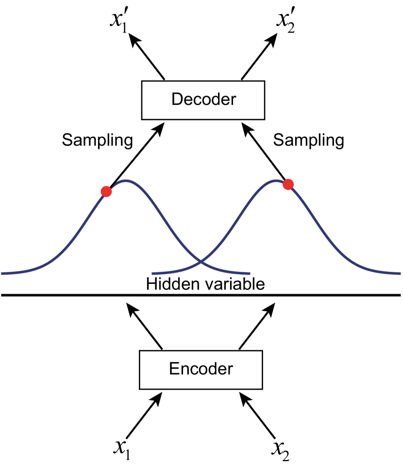
Figure 1: The data flow of VAE.

As can be observed from Eq. (5), generation error $G(z_{l})$ is actually a function of the decoder $f_{\theta}\left(z_{l}\right)$. Given $z_{l}$, the optimal decoder gives the minimal generation error. In order to obtain the extreme point, we differentiate $G(z_{l})$,

$$\frac{\partial G\left(z_{l}\right)}{\partial f_{\theta}\left(z_{l}\right)}=2\sum_{n=1}^{N}p_{\phi}(v_{n}|z_{l})\left[f_{\theta}\left(z_{l}\right)-v_{n}\right]=0\,.$$ (7)

The optimal decoder $f_{\theta}\left(z_{l}\right)$ can be obtained by letting above derivative equal to 0,

$$f_{\theta}^{*}\left(z_{l}\right)=\frac{\sum_{n=1}^{N}p_{\phi}(v_{n}|z_{l})v_{n}}{\sum_{n=1}^{N}p_{\phi}(v_{n}|z_{l})}\,\text{.}$$ (8)

where it can be clearly observed that the trained decoder is approximately the weighted average of all possible inputs.

For abnormal samples, the hidden variable $z$ should be located in the gap of the hidden variables that belongs to normal samples. The reason behinds this is intuitive: if $z$ is not in the gap of the normal hidden variables, then it must be close to one of hidden variables of the normal sample. This means that this sample is very similar to certain normal sample and it is not likely to be abnormal.

When z locates in the gap, $p_{\phi}(v_{n}|z_{l})\ll 1$, which means none of the normal value $v_{n}$ can dominate the weighted sum defined in Eq. (8). As a result, the decoder output approximates the mean-average of nearby normal samples. In unauthorized frequency bands, the access systems are various, and signals appears at random time and frequency. For certain time-frequency area, the amplitude behaves randomly over different samples, and the weighted sum defined in Eq. (8) gives a mean amplitude. As a result, the noise floor of abnormal samples is increased after reconstructed by VAE model. Instead, when z belongs to normal samples, it will locate within the realm of a normal sample. In this case, the probability weight of certain sample should be very large, decoder output approximates this normal sample.

On this basis, noise attention score is proposed to detect the abnormal spectrum usage in unauthorized frequency bands,

$$N=\sum_{i=1}^{N}\frac{\left|x_{i}-\hat{x_{i}}\right|}{x_{i}}\,,$$ (9)

where $x$ is the input amplitude of the variation encoder, $\hat{x}$ is the output amplitude of the variation encoder and $N$ is number of pixels in the spectrogram. Compared to the traditionally used reconstruction error score,

$$R=\sum_{i=1}^{N}\left|x_{i}-\hat{x_{i}}\right|\,,$$ (10)

noise attention score pays more attention to noise area (low amplitude), and is more sensitive to the noise floor change caused by abnormal spectrum usage. For this reason, noise attention score can detect abnormal spectrum more effectively and is used in our methodology.

IV Experimental results

IV-A Dataset

In this paper, ISM band is chosen as the unauthorized band for spectrum anomaly detection. The center frequency is set to be 2.4GHz and the bandwidth is set to be 25MHz. WiFi, Bluetooth and etc. are included in this observation. The USRP device is configured at a sampling rate of 50 MSamp/s with omni-directional antennas which are deployed indoors. The collected I/Q data was processed with 1024 points Short-Time Fourier Transform (STFT), and then was down-sampled with a factor of 4. The window of STFT is $1024$, the overlap is 0 and the sampling frequency is $50\mathrm{MHz}$. The size of the final spectrogram images is 64 x 64. The frequency resolution is 200 kHz, the time resolution is 80us, and the time span is 20ms.

Spectrogram data is collected for the analysis of the proposed framework over the period from 14:41:00 December 21, 2018 to 15:22:00 December 21, 2018. The collected spectrogram images are normal samples and are randomly split into training set and test set, which contains 8438 and 906 spectrogram images respectively. In order to evaluate the anomaly detection performance, anomaly samples have to be obtained by adding anomaly signal into the normal samples. Ref. [10] adopted additive white Gaussian noise as anomaly signal to simulate the anomaly case of the sudden signal-to-noise ratio change of the communication channel. Refs. [11] and [16] consider random bandwidth and SNR with deterministic shifts/hops in frequency as anomaly. In this paper , we follow Ref. [13] and define chirp signal as anomaly signal. Therefore, the test set is further equally divided into two parts. The first part consists of abnormal samples obtained by adding random chirp signals during normal use [13], while the second part remain unchanged and is labeled as normal spectrograms. Examples of the normal and abnormal spectrogram are shown in Fig. 2(a) and (b).

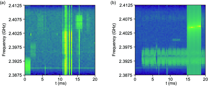
Figure 2: Spectrograms of (a) normal and (b) abnormal signals.

With the obtained dataset, the variation encoder network is trained using the train samples that are normal samples. After that, the test samples consisting of normal and abnormal signals are fed into the trained model to obtain the anomaly score. Finally, the performance of the model can be verified by Receiver Operating Characteristic (ROC) method.

IV-B Implementation details

In our study, two different architectures are adopted to investigate the performance of spectrum anomaly detection. The architectures of convolutional VAE and fully connected VAE are shown in Tab. I and Tab. II respectively. Our network is trained with Adam optimizer with $\alpha=0.001,\,\beta_{1}=0.9,\,\beta_{2}=0.999$. We train the network with batch size of 32 and implement it using Keras. It is worth noting that the VAE network is trained by normal examples in an unsupervised approach.

TABLE I: Architecture of convolutional VAE.

Section	Layer	Type	Kernel	No. of filters	Activation function
Encoder	$1,\,2,\,3$	Conv	$\left(2,\,2\right)$	$2,\,4,\,8$	LeakyReLU
	$4,\,5$	Fully connected	$4096,\,75$	-	LeakyReLU
Decoder	$1,\,2,\,3$	DeConv	$\left(2,\,2\right)$	$8,\,4,\,2$	LeakyReLU
	$4$	DeConv	$\left(2,\,2\right)$	$1$	Sigmoid

TABLE II: Architecture of fully connected VAE.

Section	Layer	Type	Kernel	No. of filters	Activation function
Encoder	$1,\,2,\,3$	Fully connected	$1024,\,256,\,64$	-	LeakyReLU
	$4$	Fully connected	$8$	-	Softplus
Decoder	$1,\,2,\,3$	Fully connected	$64,\,256,\,1024$	-	LeakyReLU
	$4$	Fully connected	$8$	-	Tanh

IV-C Noise floor change

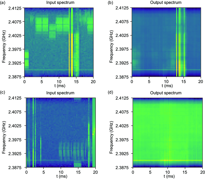
Figure 3: The input and reconstruction output of (a-b) normal spectrum, (c-d) abnormal spectrum.

In order to illustrate the noise floor change caused by abnormal spectrum usage, the reconstructed output of VAE of normal and abnormal samples are compared in Fig. 3. For abnormal spectrum, the reconstruction result has a larger noise floor compared with input, which cannot be observed in the normal case in Fig. 3 (a). This is due to the fact that the decoder output approximates the mean-average of nearby normal samples as derived in Sec. III.

IV-D ROC results

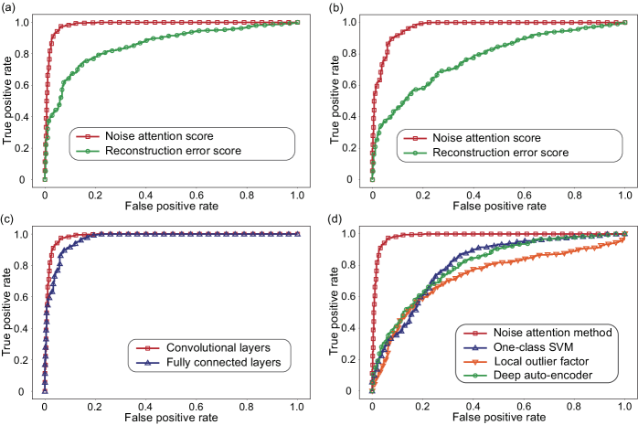
Figure 4: Performance of noise attention score on VAE with (a) convolutional layers, (b) fully connected layers. (c) Comparison between convolutional VAE and fully connected VAE. (d) Comparison of noise attention based method with traditional methods.

The performance of noise attention score is evaluated by ROC test. ROC curve examines the variation of true positive rate (TPR) with false positive rate (FPR). TPR equals the ratio of abnormal samples that are detected as abnormal. FPR equals the ratio of normal samples that are detected as abnormal, which is the false alarm rate. The Area Under Curve (AUC) index reflects the performance of the detector. The closer the AUC is to 1, the better the performance of the detector is.

The performance of noise attention score and reconstruction error score are firstly compared in convolutional VAE model. The network architecture is shown in Tab. I. The result is shown in Fig. 4(a). As can be seen, the proposed noised attention score achieves higher anomaly detection performance under same false alarm rates. AUC metrics of noise attention score and reconstruction error score are respectively 0.986 and 0.857. The performance of noise attention score is further examined in fully connected VAE model. The network architecture is shown in Tab. II. The result is shown in Fig. 4(b). The AUC metric is substantially improved by 0.193 due to the use of noise attention score.

The performance comparison of convolutional VAE model and fully connected VAE model is shown in Fig. 4(c). Noise attention score is used in both methods. The AUC metric of fully connected VAE is 0.016 lower. As can be seen, convolutional VAE model shows better performance at low FPR region, which means that convolutional VAE model can achieve lower false alarm rate for given detection rate.

Finally, we compare the proposed noise attention based method with traditional methods for spectrum anomaly detection. Three traditional methods are considered here, which includes one-class support vector machine (one-class SVM) [17], local outlier factor [18] and deep auto-encoder [19]. Convolutional VAE mode is used in noise attention based method. Experimental results are shown in Fig. 4(d). It can be clearly seen that the proposed method greatly outperforms the other methods. The AUC of these methods are summarized in Tab. III.

TABLE III: The AUC of four methods.

Model	Noise attention method	One-class SVM	Local outlier factor	Deep auto-encoder
AUC	$0.986$	$0.807$	$0.730$	$0.802$

V Conclusions

In this paper, the noise attention method is proposed for unsupervised spectrum anomaly detection in unauthorized bands, which leverages VAE to capture the spectrum data distribution and detects anomalies by selectively comparing the difference between spectrogram and its VAE reconstruction counterparts. The optimal decoder output of VAE is theoretically derived from the perspective of the minimization of generation error. It is indicated that the abnormal frequency usage will elevate the noise floor in spectrogram after VAE reconstruction. On this basis, the noise attention score is proposed for spectrum anomaly detection, which pays more attention to the background change in spectrograms. Experimental results show that noise attention score significantly increases the AUC metric by 0.193, compared with the traditional reconstruction error anomaly score. The proposed anomaly detection method is beneficial to guide spectrum sensing system to quickly filter out the high-value information from a large amount of spectrum data, and automatically invest more computing and storing resources for time-frequency window containing threatening signals.

Jing Xu received B.S. degree in Honors College from Northwestern Polytechnical University in 2018. She is currently pursuing the M.S. degree with Qian Xuesen Laboratory of Space Technology, China Academy of Space Technology, Beijing, China. Her research interests include machine learning, spectrum sensing and data mining.

Yu Tian was born in 1990 in Hebei, China. He received the Ph.D. degrees in School of Electronics Engineering and Computer Science in Peking University in 2018, and received the Bachelor degrees in School of Telecommunications Engineering in XiDian University in 2013. He is currently a Co-investigator with the Qian Xuesen Laboratory of Space Technology, Beijing, China. His current research interests include Spectrum Sharing, Signal Processing, and Deep Learing.

Shuai Yuan received the B.S. and M.S. degree from Beihang University, Beijing, China, in 2011 and 2014, respectively, both in electronic and information engineering. He is currently a research assistant in Qian Xuesen Laboratory of Space Technology, Beijing, China. His current research interests include error-control coding, spectrum sensing and processing.

Naijin Liu is the deputy director of Qian Xuesen Laboratory of Space Technology, China Academy of Space Technology, Beijing, China. He received his Ph.D. degree from China University of Science and Technology. His research interests include satellite communication and space intelligent information networking. At present, he is a council member of the Chinese Society of Astronautics.

References

- [1] S. Thombre, M. Z. H. Bhuiyan, P. Eliardsson, B. Gabrielsson, M. Pattinson, M. Dumville, D. Fryganiotis, S. Hill, V. Manikundalam, M. Poeloeskey, S. Lee, L. Ruotsalainen, S. Soderholm, and H. Kuusniemi, “Gnss threat monitoring and reporting: Past, present, and a proposed future,” Journal of Navigation, pp. 1–17, 12 2017.
- [2] M. Strohmeier, M. Schafer, R. Pinheiro, V. Lenders, and I. Martinovic, “On perception and reality in wireless air traffic communications security,” IEEE Transactions on Intelligent Transportation Systems, vol. 18, no. 6, pp. 1338–1357, 2016.
- [3] C. Salcedo Coloma and A. Garcia Armada, “Signal detection and identification for ofdm cognitive radio.” Universidad Carlos III De Madrid, 2010.
- [4] A. Ebrahimzadeh and S. A. Seyedin, “Digital signal types identification using a hierarchical svm-based classifier and efficient features,” in International Conference on Computing: Theory and Applications, 2007.
- [5] A. Gorcin and H. Arslan, “Template matching for signal identification in cognitive radio systems,” 2012.
- [6] Spectrum Monitoring. John Wiley and Sons, Ltd, 2010.
- [7] S. Liu, Y. Chen, W. Trappe, and L. J. Greenstein, “Aldo: An anomaly detection framework for dynamic spectrum access networks,” in IEEE INFOCOM 2009, 2009, pp. 675–683.
- [8] S. Liu, L. J. Greenstein, W. Trappe, and Y. Chen, “Detecting anomalous spectrum usage in dynamic spectrum access networks,” Ad Hoc Networks, vol. 10, no. 5, pp. 831–844.
- [9] S. Yin, L. Shufang, and Y. Jixin, “Temporal-spectral data mining in anomaly detection for spectrum monitoring,” 10 2009, pp. 1 – 5.
- [10] Q. Feng, Y. Zhang, C. Li, Z. Dou, and J. Wang, “Anomaly detection of spectrum in wireless communication via deep auto-encoders,” Journal of Supercomputing, 2017.
- [11] S. Rajendran, W. Meert, V. Lenders, and S. Pollin, “Unsupervised wireless spectrum anomaly detection with interpretable features,” IEEE Transactions on Cognitive Communications and Networking, pp. 1–1, 04 2019.
- [12] H. Wei, Y. Jia, and W. Lei, “Spectrum anomalies autonomous detection in cognitive radio using hidden markov models,” 2015 IEEE Advanced Information Technology, Electronic and Automation Control Conference (IAEAC 2015), vol. IEEE Advanced Information Technology, Electronic and Automation Control Conference, no. IAEAC2015, 2015.
- [13] T. O’Shea, T. Clancy, and R. Mcgwier, “Recurrent neural radio anomaly detection,” 11 2016.
- [14] Z. Li, Z. Xiao, B. Wang, B. Zhao, and H. Zheng, “Scaling deep learning models for spectrum anomaly detection,” 07 2019, pp. 291–300.
- [15] D. Kingma and M. Welling, “Auto-encoding variational bayes,” 12 2014.
- [16] S. Rajendran, V. Lenders, W. Meert, and S. Pollin, “Crowdsourced wireless spectrum anomaly detection,” 2019.
- [17] B. Schlkopf, R. C. Williamson, A. J. Smola, J. Shawe-Taylor, and J. C. Platt, “Support vector method for novelty detection,” in Advances in Neural Information Processing Systems 12, NIPS Conference, Denver, Colorado, USA, November 29 - December 4, 1999, 1999.
- [18] M. Breunig, H.-P. Kriegel, R. Ng, and J. Sander, “Lof: Identifying density-based local outliers.” vol. 29, 06 2000, pp. 93–104.
- [19] G. E. Hinton and R. S. Zemel, “Autoencoders, minimum description length and helmholtz free energy,” Advances in Neural Information Processing Systems, vol. 6, 1993.