Budgeted Influence and Earned Benefit Maximization with Tags in Social Networks

Abstract

Given a social network, where each user is associated with a selection cost, the problem of Budgeted Influence Maximization (BIM Problem in short) asks to choose a subset of them (known as seed users) within an allocated budget whose initial activation leads to the maximum number of influenced nodes. Existing Studies on this problem do not consider the tag-specific influence probability. However, in reality, influence probability between two users always depends upon the context (e.g., sports, politics, etc.). To address this issue, in this paper we introduce the Tag-Based Budgeted Influence Maximization problem (TBIM Problem in short), where along with the other inputs, a tag set (each of them is also associated with a selection cost) is given, each edge of the network has the tag specific influence probability, and here the goal is to select influential users as well as influential tags within the allocated budget to maximize the influence. Considering the fact that real-world campaigns targeted in nature, we also study the Earned Benefit Maximization Problem in tag specific influence probability setting, which formally we call the Tag-Based Earned Benefit Maximization problem (TEBM Problem in short). For this problem along with the inputs of the TBIM Problem, we are given a subset of the nodes as target users, and each one of them is associated with a benefit value that can be earned by influencing them. Considering the fact that different tag has different popularity across the communities of the same network, we propose three methodologies that work based on effective marginal influence gain computation. The proposed methodologies have been analyzed for their time and space requirements. We evaluate the methodologies with three publicly available social network datasets, and observe, that these can select seed nodes and influential tags, which leads to more number of influenced nodes and more amount of earned benefit compared to the baseline methods.

1 Introduction

A social network is an interconnected structure among a group of agents formed for social interactions Carrington et al. [2005]. One of the important phenomena of social networks is the diffusion of information. Based on the diffusion process, a well-studied problem in the domain of computational social network analysis is the Social Influence Maximization (SIM Problem), which has an immediate application in the context of viral marketing. The goal here is to get wider publicity for a product by initially distributing a limited number of free samples to highly influential users. For a given social network and a positive integer $k$, the SIM Problem asks to select $k$ users for initial activation to maximize the influence in the network. Due to potential application across multiple domains such as personalized recommendation Zhang et al. [2013], feed ranking Ienco et al. [2010], viral marketing Chen et al. [2010], this problem remains the central theme of research since last one and half decades or so. Please look into Li et al. [2018b], Peng et al. [2018], Banerjee et al. [2020b] for recent surveys.

Recently, a variant of this problem has been introduced by Nguyen and Zheng Nguyen and Zheng [2013], where the users of the network are associated with a selection cost and the seed set selection is to be done within an allocated budget to maximize the influence in the network. There are a few solution methodologies of the problem such as directed acyclic graph (DAG)-based heuristics and $(1-\frac{1}{\sqrt{e}})$-factor approximation algorithm by Nguyen and Zheng [2013], balanced seed selection heuristics by Han et al. [2014], integer programming-based approach Güney [2017], community-based solution approach by Banerjee et al. [2019a]. In all these studies it is implicitly assumed that irrespective of the context, influence probability between two users will be the same, i.e., there is a single influence probability associated with every edge. However, in reality, the scenario is different. It is natural that a sportsman can influence his friend in any sports related news with more probability compared to political news. This means the influence probability between any two users is context specific, and hence, in Twitter, a follower will re-tweet if the tweet contains some specific hash tags. To address this issue, in this paper we introduce the Tag-based Budgeted Influence Maximization Problem (TBIM Problem), which considers the tag specific influence probability assigned with every edge of the network.

Consider the case of a commercial campaign, where an E-Commerce house promotes its newly developed product. It is quite natural that not all the customers present in their database will be interested in the product. Hence, it is not really beneficial to advertise a product to a user, if he is not at all interested and this can be easy to predict from his browsing/liking/rating history. This implies that the advertisement needs to be conducted among the group of target users. It is quite natural that the target users are associated with a benefit value that can be earned by the E-Commerce house by influencing the corresponding user. Hence, in a targeted advertisement setting the natural problem is that given a social network where every user is associated with a selection cost, a set of target users with a benefit value. The goal here is to choose a seed set within the allocated budget to maximize the earned benefit by influencing the target users. Formally, this problem has been referred to as the Earned Benefit Maximization Problem Banerjee et al. [2020a]. There are several studies by Banerjee et al. Banerjee et al. [2020a, 2019b, 2019c] and also by several other authors as well in this direction Tang et al. [2017], Zhu et al. [2017], Zhou et al. [2019]. However, none of these studies considers the tag specific influence probability, though it is a practical concern as mentioned previously. In this paper, we study this problem in tag specific influence probability setting and formally call as Tag-Based Earned Benefit Maximization Problem (TEBM Problem).

Recently, Ke et al. [2018] studied the problem of finding $k$ seed nodes and $r$ influential tags in a given social network. However, their study has two drawbacks. First, in reality, most of the social networks are formed by rational human beings. Hence, once a node is selected as a seed then incentivization is required (e.g., free or discounted sample of the item to be advertised). In practical cases, E-Commerce houses hire some online social media platforms to run the commercial campaign. The message for this purpose may be composed of many animations, videos, images, and also texts (together referred to as tags). To display a tag in an on-line advertisement also associated with some cost. Hence, online social media platforms will charge money based on the tags present in the message. So, the tags that have been used to construct the message will also be associated with a selection cost. Their study does not consider these issues. Secondly, in Ke et al. [2018]’s study, they have done the tag selection process at the network level. However, in reality, popular tags may vary from one community to another in the same network. Figure 1 shows community-wise distribution of Top $5$ tags for the Last.fm dataset. From the figure, it is observed that Tag No. $16$ has the highest popularity in Community $3$. However, its popularity is very less in Community $4$. This signifies that tag selection at the network level may not be always helpful to spread influence in each community of the network. To mitigate these issues, in this paper, we propose three solution methodologies for the TBIM Problem, where the tag selection is done community-wise. To summarize, the main contributions of this paper are as follows:

• Considering the tag specific influence probability, in this paper, we introduce the Tag-Based Budgeted Influence Maximization Problem (TBIM Problem) and Tag-Based Earned Benefit Maximization Problem.

• For both these problems, we propose two different marginal influence gain-based approaches with their detailed analysis.

• To increase the scalability of the proposed methodologies, we propose an efficient pruning technique.

• The proposed methodologies have been implemented with three publicly available datasets and a set of experiments have been performed to show their effectiveness.

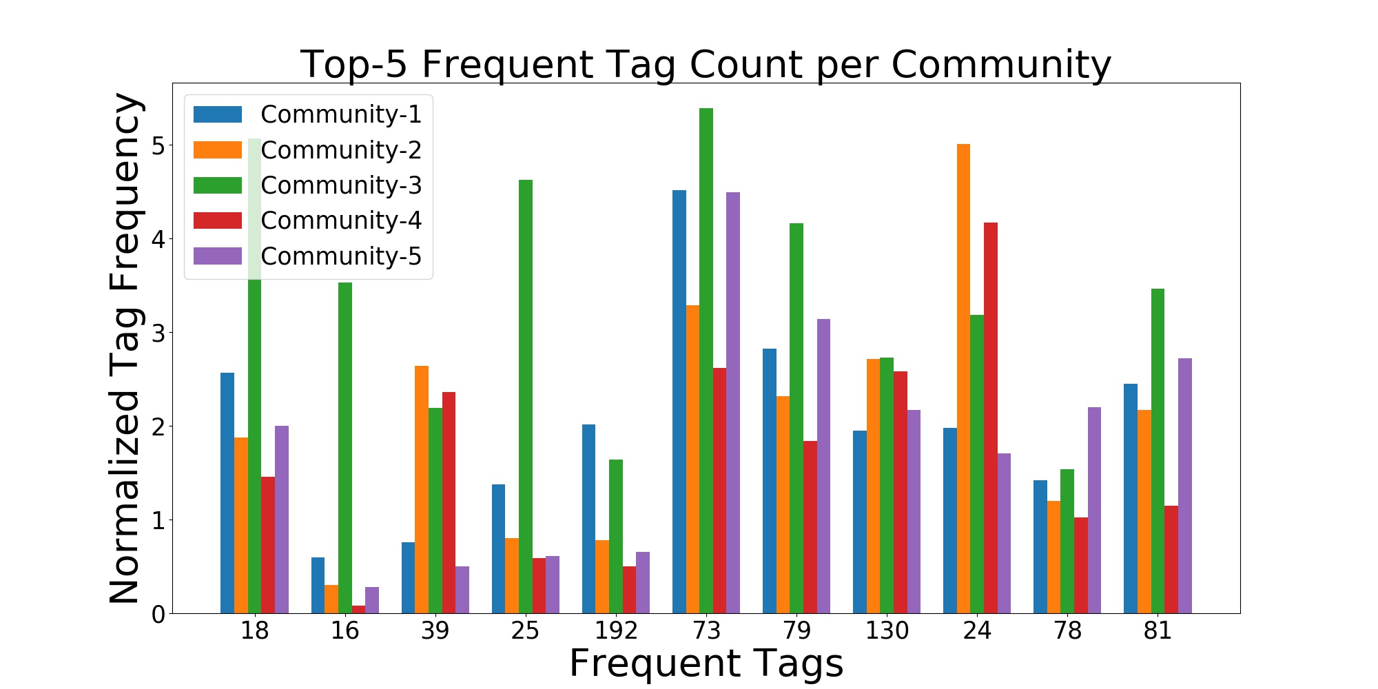
Figure 1: Community specific distribution top 5 tags in ‘Last.fm’ dataset

The rest of the paper is arranged as follows: Section 2 discusses some relevant studies from the literature. Section 3 contains some background material and defines the TBIM Problem formally. The proposed solution methodologies for this problem have been described in Section 4. In Section 5, we report the experimental results of the proposed methodologies. Finally, Section 6 concludes of our study.

2 Related Work

Our study is related to the Social and Budgeted Influence maximization, Keyword-Based Influence Maximization and Community-Based Solution Methodologies for the Influence Maximization. Here we describe them one by one.

Social/Budgeted Influence maximization

Given a social network and positive integer $k$, the problem of Social Influence Maximization asked to select Top-k influential users in the network for initial activation to maximize the influence. This problem has been initially proposed by Domingos and Richardson [2001] in the context of viral marketing. Later, Kempe et al. [2003] resolves the complexity issues of this problem and proposed an incremental greedy strategy that admits $(1-\frac{1}{e})$- factor approximation guarantee. This study triggers extensive research work and hence, a vast amount of literature is available. Most of the solution methodologies are concerned either about the quality of the selected seed set (i.e., the optimality gap) or about the scalability issues (i.e., when the problem size increases how the computational time changes). Proposed solution methodologies can be classified into different categories such as approximation algorithms (e.g., CELF Leskovec et al. [2007], CELF++ Goyal et al. [2011], MIA and PMIA Wang et al. [2012]), sketch-based approaches (e.g., TIM Tang et al. [2014], IMM Tang et al. [2015]), heuristic approaches (e.g., SPIN Narayanam and Narahari [2011], ASIM Galhotra et al. [2015] and many more), soft computing-based approaches (GA Bucur and Iacca [2016] Zhang et al. [2017], PSO Gong et al. [2016]) and so on.

Recently, a variant of the SIM Problem has been introduced by Nguyen and Zheng [2013], where the nodes of the network are associated with a selection cost and the goal is to select a subset of the nodes within an allocated budget for initial activation to maximize the influence. This Problem is known as the Budgeted Influence Maximization Problem. Available solution methodologies for this problems are as follows. Nguyen and Zheng [2013] proposed a $(1-\frac{1}{\sqrt{e}})$-factor approximation algorithm and two DAG-based heuristics for the BIM Problem. Han et al. [2014] proposed a set of heuristics considering both influential nodes and also cost effective nodes. Güney [2017] proposed an integer programming-based approach under the independent cascade model of diffusion. Recently, Banerjee et al. [2019a] proposed a community-based solution approach for this problem. However, none of these studies consider the tag-specific influence probability.

Tag/Keyword-Based Influence Maximization

As mentioned previously, keywords are important in the case of online advertising. There are a few studies available, where keyword-based influence probabilities have been taken into consideration. Li et al. [2015] studied the SIM Problem, where the goal is to select a subset of the users (known as target users). Recently, Ke et al. [2018] studied the problem for finding the seed nodes and initial tag set jointly and they proposed heuristic solutions for this problem. Fan et al. [2018] developed an online topic-based influence analysis system that discovers keyword-based influential users in the network as one of its tasks with two others. However, none of these studies consider the selection cost of the tags, which is a practical concern as mentioned earlier.

Community-based Influence Maximization

As the real-world social networks are gigantic in size and pose a strong community structure, recently several methods have been proposed where the community structure of the network has been exploited. In this direction, the first study was made by Wang et al. [2010] Chen et al. [2012, 2014], and their method outperforms many existing methods in terms of scalability and efficiency. Bozorgi et al. [2016] proposed a community-based approach under the linear threshold diffusion model, where the goal is to find influential communities by considering the global influence of the users. Shang et al. [2017] proposed a community-based framework that leads to acceptable computational time for large scale networks. Bozorgi et al. [2017] proposed a solution methodology using the community structure of the network under the competitive linear threshold model. Hosseini-Pozveh et al. [2017] proposed a community-based approach that shows a balance between between effectiveness and efficiency. Recently, there are several studies in this direction Huang et al. [2019], Li et al. [2018a], Singh et al. [2019].

Benefit/Profit Maximization using Social Networks

In recent times there are several studies that focus on benefit/profit maximization in online social networks Tong et al. [2018], Tang et al. [2017], Huang et al. [2020]. Tong et al. [2018] considered the coupon allocation problem in profit maximization. By utilizing the double greedy algorithm proposed by Buchbinder et al. [2015], they showed that their proposed approaches can achieve $\frac{1}{2}$-factor approximation guarantee with high probability. Later, Liu et al. [2020] also studied this problem under the independent cascade model with coupon and valuation and proposed the PMCA Algorithm based on a local search technique proposed in Feige et al. [2011]. If the submodular profit function is non-negative for every subset of the users, then PMCA can achieve an approximation ratio $\frac{1}{3}$. Tang et al. [2017] studied the profit maximization problem and proposed two different approaches for solving this problem; namely an incremental greedy hill-climbing approach, and a double greedy algorithm.

In this paper, we propose three solution methodologies for the TBIM and TEBM Problem, which exploits the community structure of the network.

3 Background and Problem Definition

We assume that the input social network is represented as a directed and edge-weighted graph $\mathcal{G}(\mathcal{V},\mathcal{E},\mathcal{P})$, where the vertex set, $\mathcal{V}(\mathcal{G})=\{u_{1},u_{2},\ldots,u_{n}\}$ is the set of $n$ users, the edge set $\mathcal{E}(\mathcal{G})=\{e_{1},e_{2},\ldots,e_{m}\}$ is the set of $m$ social ties among the users. Along with $\mathcal{G}$, we are also given with a tag set $T=\{t_{1},t_{2},\ldots,t_{a}\}$ relevant to the users of the network. Here, $\mathcal{P}$ is the edge weight function that assigns each edge to its tag-specific influence probability, i.e., $\mathcal{P}:\mathcal{E}(\mathcal{G})\longrightarrow(0,1]^{|T|}$. This means that each edge of the network is associated with an influence probability vector, whose each dimension is for a particular tag. For all $(u_{i}u_{j})\in\mathcal{E}(\mathcal{G})$, we denote its corresponding influence probability vector as $\mathcal{P}_{u_{i}\rightarrow u_{j}}$. Also, for a particular tag $t\in T$ and an edge $(u_{i}u_{j})\in\mathcal{E}(\mathcal{G})$, we denote the influence probability of the edge $(u_{i}u_{j})$ for the tag $t$ as $\mathcal{P}_{u_{i}\rightarrow u_{j}}^{t}$. This can be interpreted as the conditional probability of the edge $(u_{i}u_{j})$ given the tag $t$, i.e., $\mathcal{P}_{u_{i}\rightarrow u_{j}}^{t}=Pr((u_{i}u_{j})|t)$. Now, a subset of the available tags $T^{{}^{\prime}}\subseteq T$ which are relevant to the campaign may be used. So, it is important how to compute the effective probability for each edge and this depends upon how the selected tags are aggregated. In this study, we perform the independent tag aggregation, which is defined as follows.

Definition 1 (Independent Tag Aggregation).

Given a social network $\mathcal{G}(\mathcal{V},\mathcal{E},\mathcal{P})$, the tag set $T^{{}^{\prime}}\subseteq T$, the aggregated influence probability of the edge $(u_{i}u_{j})$ can be computed as follows:

$$\mathcal{P}_{u_{i}\rightarrow u_{j}}^{T^{{}^{\prime}}}=1-\underset{t\in T^{{}^{\prime}}}{\prod}(1-\mathcal{P}_{u_{i}\rightarrow u_{j}}^{t})$$ (1)

Now, to conduct a campaign using a social network, a subset of the users need to be selected initially as seed nodes. The number of influenced nodes will depend upon which influence propagation model we are using. In our study, we assume that the influence is propagated based on the Maximum Influence Arborance (MIA) diffusion model, which is discussed next.

Diffusion in Social Networks

We denote the seed set by $\mathcal{S}$. The users in the set $\mathcal{S}$ are informed initially, and the others are ignorant about the information. These seed users start the diffusion, and the information is diffused by the rule of an information diffusion model. There are many such rules proposed in the literature. One of them is the MIA Model [Wang et al., 2012]. Recently, this model has been used by many existing studies in influence maximization [Chen et al., 2011]. In our study also, we assume that the information is diffused by the rule of MIA Model. Before defining the MIA Model, we first state a few preliminary definitions.

Definition 2 (Propagation Probability of a Path).

Given two vertices $u_{i},u_{j}\in V(\mathcal{G})$, let $\mathbb{P}(u_{i},u_{j})$ denotes the set of paths from the vertex $u_{i}$ to $u_{j}$. For any arbitrary path $p\in\mathbb{P}(u_{i},u_{j})$ the propagation probability is defined as the product of the influence probabilities of the constituent edges of the path.

$$\mathcal{P}(p)=\begin{cases}\underset{(u_{i}u_{j})\in\mathcal{E}(p)}{\prod}\mathcal{P}^{T^{{}^{\prime}}}_{u_{i}\rightarrow u_{j}}&\text{if $\mathbb{P}(u_{i},u_{j})\neq\phi$}\\ 0&\text{otherwise}\\ \end{cases}$$ (2)

Here, $\mathcal{E}(p)$ denotes the edges that constitute the path $p$.

Definition 3 (Maximum Probabilistic Path).

Given two vertices $u_{i},u_{j}\in\mathcal{V}(\mathcal{G})$, the maximum probabilistic path is the path with the maximum propagation probability and denoted as $p_{(u_{i}u_{j})}^{max}$. Hence,

$$p_{(u_{i}u_{j})}^{max}=\underset{p\in\mathbb{P}(u_{i},u_{j})}{argmax}\ \mathcal{P}(p)$$ (3)

Definition 4 (Maximum Influence In Arborence).

For a given threshold $\theta$, the maximum influence in-arborence of a node $v\in\mathcal{V}(\mathcal{G})$ is defined as

$$MIIA(v,\theta)=\underset{u\in\mathcal{V}(\mathcal{G}),\mathcal{P}(p_{(uv)}^{max})\geq\theta}{\bigcup}p_{(uv)}^{max}$$ (4)

Given a seed set $\mathcal{S}$ and a node $v\notin\mathcal{S}$, in MIA Model, the influence from $\mathcal{S}$ to $v$ is approximated by the rule that for any $u\in\mathcal{S}$ can influence $v$ through the paths in $p_{(uv)}^{max}$. The influence probability of a node $u\in MIIA(v,\theta)$ is denoted as $ap(u,\mathcal{S},MIIA(v,\theta))$, which is the probability that the node $u$ will be influenced by the nodes in $\mathcal{S}$ and influence is propagated through the paths in $MIIA(v,\theta)$. This can be computed by Algorithm 2, given in [Wang et al., 2012]. Hence, the influence spread obtained by the seed set $\mathcal{S}$ is given by Equation 5.

$$\sigma(\mathcal{S})=\underset{v\in\mathcal{V}(\mathcal{G})}{\sum}ap(v,\mathcal{S},MIIA(v,\theta))$$ (5)

Problem Definition

To study the BIM Problem along with the input social network, we are given with the selection costs of the users which is characterized by the cost function $\mathcal{C}:\mathcal{V}(\mathcal{G})\rightarrow\mathbb{R}^{+}$, and a fixed budget $\mathcal{B}$. For any user $u\in\mathcal{V}(\mathcal{G})$, its selection cost is denoted as $\mathcal{C}(u)$. Now, we define the BIM Problem formally.

Definition 5 (BIM Problem).

Given a social network $\mathcal{G}(\mathcal{V},\mathcal{E},\mathcal{P})$, the cost function $\mathcal{C}:\mathcal{V}(\mathcal{G})\rightarrow\mathbb{R}^{+}$, and an allocated budget $\mathcal{B}$, the BIM Problem asks to select a subset of the nodes $\mathcal{S}$ for initial activation to maximize $\sigma(\mathcal{S})$ such that $\underset{u\in\mathcal{S}}{\sum}\mathcal{C}(u)\leq\mathcal{B}$.

Now, as mentioned previously, tags are important in any kind of campaign also popularity of tags varies across the communities of a network. Assume that the input social network has $p$ number of communities, i.e., the community set is $\mathcal{K}=\{\mathcal{K}_{1},\mathcal{K}_{2},\ldots,\mathcal{K}_{\ell}\}$. Naturally, all the tags that are considered in a specific context (i.e., $T$) may not be relevant to each of the communities. We denote the relevant tags of the community $\mathcal{K}_{i}$ as $T_{\mathcal{K}_{i}}$. It is important to observe that displaying a tag in any online platform may associate some cost, which can be characterized by the tag cost function $\mathcal{C}^{T}:T\rightarrow\mathbb{R}^{+}$. Now, for a set of given tags and seed nodes what will be the number of influenced nodes in the network? This can be defined as the tag-based influence function. For a given seed set $\mathcal{S}$ and tag set $T^{{}^{\prime}}$, the tag-based influence function $\sigma(\mathcal{S},T^{{}^{\prime}})$ returns the number of influenced nodes, which is defined next.

Definition 6 (Tag-based Influence Function).

Given a social network $\mathcal{G}(\mathcal{V},\mathcal{E},\mathcal{P})$, a seed set $\mathcal{S}\subseteq\mathcal{V}(\mathcal{G})$, tag set $T^{{}^{\prime}}\subseteq T$, the tag-based influence function $\sigma^{\mathcal{T}}$ that maps each combination of subset of the nodes and tags to the number of influenced nodes, i.e., $\sigma^{\mathcal{T}}:2^{\mathcal{V}(\mathcal{G})}\times 2^{T}\longrightarrow\mathbb{R}_{0}$.

In this paper, we introduce the Tag-based Budgeted Influence Maximization Problem (TBIM Problem) and Tag-based Earned Benefit Maximization Problem (TEBM Problem), which we define next.

Definition 7 (TBIM Problem).

Given a social network $\mathcal{G}(\mathcal{V},\mathcal{E},\mathcal{P})$, Tag set $T$, seed cost function $\mathcal{C}^{S}:\mathcal{V}(\mathcal{G})\rightarrow\mathbb{R}^{+}$, tag cost function $\mathcal{C}^{T}:T\rightarrow\mathbb{R}^{+}$ and the budget $\mathcal{B}$, the TBIM Problem asks to select a subset of the tags from the communities, i.e., $T_{\mathcal{K}_{i}}^{{}^{\prime}}\subseteq T_{\mathcal{K}_{i}}$, $\forall i\in[\ell]$ (here, $T_{\mathcal{K}_{i}}^{{}^{\prime}}\cap T_{\mathcal{K}_{j}}^{{}^{\prime}}=\emptyset,\ \forall i\neq j\text{ and }T^{{}^{\prime}}=\underset{i\in[l]}{\bigcup}T_{\mathcal{K}_{i}}$), and nodes $\mathcal{S}\subseteq\mathcal{V}(\mathcal{G})$ to maximize $\sigma^{\mathcal{T}}(\mathcal{S},T^{{}^{\prime}})$ such that $\underset{u\in\mathcal{S}}{\sum}\mathcal{C}^{S}(u)+\underset{i\in[\ell]}{\sum}\ \underset{t\in T_{\mathcal{K}_{i}}}{\sum}\mathcal{C}^{T}(t)\leq\mathcal{B}$.

Mathematically, the TBIM Problem can be posed as follows:

$$(\mathcal{S}^{*},T^{*})=\underset{(\mathcal{S},T^{{}^{\prime}});\\ \mathcal{S}\subseteq\mathcal{V}(\mathcal{G}),T^{{}^{\prime}}\subseteq T;\mathcal{C}^{S}(\mathcal{S})+\mathcal{C}^{T}(T^{{}^{\prime}})\leq\mathcal{B}}{argmax}\ \sigma^{\mathcal{T}}(\mathcal{S},T^{{}^{\prime}})$$ (6)

From the algorithmic point of view the TBIM Problem can be posed as follows:

As mentioned previously, in many real-world campaigns, the goal is to not just to maximize the influence, but also to maximize the total earned benefit by influencing the target users. Assume that $\mathcal{D}\subseteq\mathcal{V}(\mathcal{G})$ is the set of target users and $b:\mathcal{D}\longrightarrow\mathbb{R}^{+}$ is the benefit function that assigns each target user to its benefit that can be earned by influencing the corresponding target user, $\mathcal{C}:\mathcal{V}(\mathcal{G})\longrightarrow\mathbb{R}^{+}$ is the cost function of the users, and $\mathcal{B}$ is the allocated budget for the seed set selection. Let, $b(u)$ denotes the associated benefit with the user $u$. Now, we define the earned benefit by a seed set.

Definition 8 (Earned Benefit by a Seed Set).

Given a seed set $\mathcal{S}$, its earned benefit is denoted as $\beta(\mathcal{S})$ and defined as

$$\beta(\mathcal{S})=\underset{u\in\mathcal{D}\cap I(\mathcal{S})}{\sum}b(u).$$ (7)

Here, $\beta(.)$ is the earned benefit function that assigns each subset to its earned benefit that assigns each subset of its user to its earned benefit; i.e.; $\beta:2^{\mathcal{V}(\mathcal{G})}\longrightarrow\mathbb{R}^{+}$ with $\beta(\emptyset)=0$.

As in this study, we are studying the TEBM Problem in tag specific influence probability setting, it is worthwhile to consider the Tag-Based Earned Benefit Function, which can be defined equivalently as the tag-based social influence function is defined in Definition 6. Now, the goal of the Tag-based Earned Benefit Maximization Problem is to choose influential users and tags to maximize the earned benefit stated in Definition 9.

Definition 9 (Tag-Based Earned Benefit Maximization Problem).

Given a social network $\mathcal{G}(\mathcal{V},\mathcal{E},\mathcal{P})$, target user seed $\mathcal{D}$, benefit function $b:\mathcal{D}\longrightarrow\mathbb{R}^{+}$, Tag set $T$, seed cost function $\mathcal{C}^{S}:\mathcal{V}(\mathcal{G})\longrightarrow\mathbb{R}^{+}$, tag cost function $\mathcal{C}^{T}:T\longrightarrow\mathbb{R}^{+}$ and the budget $\mathcal{B}$, the TEBM Problem asks to select a subset of the tags from the communities, i.e., $T_{\mathcal{K}_{i}}^{{}^{\prime}}\subseteq T_{\mathcal{K}_{i}}$, $\forall i\in[\ell]$ (here, $T_{\mathcal{K}_{i}}^{{}^{\prime}}\cap T_{\mathcal{K}_{j}}^{{}^{\prime}}=\emptyset,\ \forall i\neq j\text{ and }T^{{}^{\prime}}=\underset{i\in[\ell]}{\bigcup}T_{\mathcal{K}_{i}}$), and nodes $\mathcal{S}\subseteq\mathcal{V}(\mathcal{G})$ to maximize $\beta^{\mathcal{T}}(\mathcal{S},T^{{}^{\prime}})$ such that $\underset{u\in\mathcal{S}}{\sum}\mathcal{C}^{S}(u)+\underset{i\in[\ell]}{\sum}\ \underset{t\in T_{\mathcal{K}_{i}}}{\sum}\mathcal{C}^{T}(t)\leq\mathcal{B}$.

Mathematically, the TEBM Problem can be posed as follows:

$$(\mathcal{S}^{*},T^{*})=\underset{(\mathcal{S},T^{{}^{\prime}});\\ \mathcal{S}\subseteq\mathcal{V}(\mathcal{G}),T^{{}^{\prime}}\subseteq T;\mathcal{C}^{S}(\mathcal{S})+\mathcal{C}^{T}(T^{{}^{\prime}})\leq\mathcal{B}}{argmax}\ \beta^{\mathcal{T}}(\mathcal{S},T^{{}^{\prime}})$$ (8)

From the computational point of view, the TEBM Problem can be defined as follows:

Symbols that have been used in this paper is shown in Table 1.

Table 1: Symbols with their interpretation

Symbol	Interpretation
$\mathcal{G}(\mathcal{V},\mathcal{E},\mathcal{P})$	The input social network
$\mathcal{V}(\mathcal{G}),\mathcal{E}(\mathcal{G})$	The vertex set and edge set of $\mathcal{G}$
$\mathcal{D}$	The set of target users
$T$	The tag set
$\mathcal{P}$	The edge weight function $\mathcal{P}:\mathcal{E}(\mathcal{G})\times T\longrightarrow(0,1]^{|T|}$
$\mathcal{P}_{u_{i}\rightarrow u_{j}}$	The influence probability vector from the user $u_{i}$ to $u_{j}$
$\mathcal{P}_{u_{i}\rightarrow u_{j}}^{t}$	The influence probability from the user $u_{i}$ to $u_{j}$ for the tag $t$
$\mathcal{C}^{S}$, $\mathcal{C}^{T}$	The cost function for the users and tags
$\mathcal{C}^{S}(u)$, $\mathcal{C}^{T}(t)$	The selection cost for the user $u$, and tag $t$, respectively
$b$	Benefit function for target user
$b(u)$	Benefit of the user $u$
$\beta$	Earned benefit function
$\beta(\mathcal{S})$	Earned benefit by the seed set $\mathcal{S}$
$\mathcal{B}$	Allocated budget for the seed nodes and tag selection
$\mathcal{K}$	Set of communities of $\mathcal{G}$
$\ell$	The number of communities of $\mathcal{G}$, i.e., $|\mathcal{K}|=\ell$
$\pi_{i}$	Priority of the $i$-th community
$\mathbb{P}(u_{i},u_{j})$	Set of paths between $u_{i}$, and $u_{j}$
$\mathbb{R}^{+}$	Set of positive real number
$\mathbb{R}_{0}$	Set of positive real number including $0$
$\sigma(.)$	The social influence function
$\sigma^{\mathcal{T}}(.)$	The tag-based social influence function
$\delta_{v}$, $\delta_{t}$	Effective Marginal Influence Gain for the user $u$ and tag $t$
$\delta_{(v,t)}$	Effective Marginal Influence Gain for the user-tag pair $(v,t)$

4 Proposed Methodologies

In this section, we propose two different approaches and one subsequent improvement to select tags and seed users for initiating the diffusion process. Before stating the proposed solution approaches, we first define the Effective Marginal Influence Gain.

Definition 10 (Effective Marginal Influence Gain).

Given a seed set $\mathcal{S}\subset\mathcal{V}(\mathcal{G})$, tag set $T^{{}^{\prime}}\subset T$, the effective marginal influence gain (EMIG, henceforth) of the node $v\in\mathcal{V}(\mathcal{G})\setminus\mathcal{S}$ (denoted as $\delta_{v}$) with respect to the seed set $\mathcal{S}$ and tag set $T^{{}^{\prime}}$ is defined as the ratio between the marginal influence gain to its selection cost, i.e.,

$$\delta_{v}=\frac{\sigma^{\mathcal{T}}(\mathcal{S}\cup\{v\},T^{{}^{\prime}})-\sigma^{\mathcal{T}}(\mathcal{S},T^{{}^{\prime}})}{\mathcal{C}^{S}(v)}.$$ (9)

In the similar way, for any tag $t\in T\setminus T^{{}^{\prime}}$, its EMIG is defied as

$$\delta_{t}=\frac{\sigma^{\mathcal{T}}(\mathcal{S},T^{{}^{\prime}}\cup\{t\})-\sigma^{\mathcal{T}}(\mathcal{S},T^{{}^{\prime}})}{\mathcal{C}^{T}(t)}.$$ (10)

For the user-tag pair $(v,t)$, $v\in\mathcal{V}(\mathcal{G})\setminus\mathcal{S}$, and $t\in T\setminus T^{{}^{\prime}}$, its EMIG is defined as

$$\delta_{(v,t)}=\frac{\sigma^{\mathcal{T}}(\mathcal{S}\cup\{v\},T^{{}^{\prime}}\cup\{t\})-\sigma^{\mathcal{T}}(\mathcal{S},T^{{}^{\prime}})}{\mathcal{C}^{S}(v)+\mathcal{C}^{T}(t)}.$$ (11)

Now we proceed to describe the proposed methodologies for solving the TBIM Problem.

4.1 Methodologies Based on Effective Marginal Influence Gain Computation of User-Tag Pairs (EMIG-UT)

In this approach, initially, the community structure of the network is detected and then the total allocated budget for seed selection is divided among the communities based on its size (i.e., number of nodes present in it). In each community, the shared budget is divided into two halves to be utilized to select tags and seed nodes, respectively. Next, we sort the communities based on their size in ascending order. Now, we take the smallest community first and select the most frequent tag which is less than or equal to the budget. Next, each community from smallest to the largest is processed for tag and seed node selection in the following way. Until the budget for both tag and seed node selection is exhausted, in each iteration the user-tag pair that causes maximum EMIG value is chosen and kept into the seed set and tag set, respectively. The extra budget for which no tag and no seed node can be selected is transferred to the largest community. Algorithm 1 describes the entire procedure.

Data: Social Network $\mathcal{G}(\mathcal{V},\mathcal{E},\mathcal{P})$, Tag Set $T$, Node Cost Function $\mathcal{C}^{S}:\mathcal{V}(\mathcal{G})\longrightarrow\mathbb{R}^{+}$, User-Tag Count Matrix $\mathcal{M}$, Tag Cost Function $\mathcal{C}^{T}:T\longrightarrow\mathbb{R}^{+}$, Budget $\mathcal{B}$

Result: Seed set $\mathcal{S}\subseteq\mathcal{V}(\mathcal{G})$, and Tag set $T^{{}^{\prime}}\subseteq T$

1 $\mathcal{S}=\emptyset$; $T^{{}^{\prime}}=\emptyset$ ;

2 $Community=Community\_Detection(\mathcal{G})$;

3 $\mathcal{K}\longleftarrow\{\mathcal{K}_{1},\mathcal{K}_{2},\dots,\mathcal{K}_{\ell}\}$;

4 $\mathcal{K}_{max}=Largest\_Community(\mathcal{K})$;

5 $T_{\mathcal{K}}=Crete\_Matrix(|\mathcal{K}|,|T|,0)$;

6 $T_{\mathcal{K}}=\text{Count the tag frequencies in each communities}$;

7 $\text{Sort row of }T_{\mathcal{K}}\text{corresponding to the smallest community }$;

8 $Create\_Vector(\mathcal{B}^{k}_{\mathcal{S}},\ell,0)$;

9 $Create\_Vector(\mathcal{B}^{k}_{T},\ell,0)$;

10 for $i=1\text{ to }|\mathcal{K}|$ do

11       $\mathcal{B}^{k}=\frac{|\mathcal{V}_{\mathcal{K}_{i}}|}{n}.\mathcal{B}$;

12       $\mathcal{B}^{k}_{\mathcal{S}}[i]=\frac{\mathcal{B}^{k}}{2}$; $\mathcal{B}^{k}_{T}[i]=\frac{\mathcal{B}^{k}}{2}$;

13      

14 end for

15$\mathcal{K}=Sort(\mathcal{K})$;

16 $T^{{}^{\prime}}=T^{{}^{\prime}}\cup\{t^{{}^{\prime}}:t^{{}^{\prime}}\text{ is most frequent in }\mathcal{K}_{1}\text{ and }\mathcal{C}(t)\leq\mathcal{B}^{k}_{T}[i]\}$;

17 $\mathcal{B}^{k}_{T}[1]=\mathcal{B}^{k}_{T}[1]-\mathcal{C}^{T}(t^{{}^{\prime}})$;

18 for $i=1\text{ to }|\mathcal{K}|$ do

19       while $\mathcal{B}^{k}_{\mathcal{S}}[i]>0\text{ and }\mathcal{B}^{k}_{T}[i]>0$ do

20             $(u,t)=\underset{t^{{}^{\prime\prime}}\in T\setminus T^{{}^{\prime}},\mathcal{C}(t^{{}^{\prime\prime}})\leq\mathcal{B}^{k}_{T}[i]}{\underset{v\in\mathcal{V}_{\mathcal{K}_{i}}(\mathcal{G})\setminus\mathcal{S},\mathcal{C}(v)\leq\mathcal{B}^{k}_{\mathcal{S}}[i];}{argmax}}\delta_{(v,t^{{}^{\prime\prime}})}$;

21             $\mathcal{S}=\mathcal{S}\cup\{u\};T^{{}^{\prime}}=T^{{}^{\prime}}\cup\{t\}$;

22             $\mathcal{B}^{k}_{\mathcal{S}}[i]=\mathcal{B}^{k}_{\mathcal{S}}[i]-\mathcal{C}^{S}(u);\mathcal{B}^{k}_{T}[i]=\mathcal{B}^{k}_{T}[i]-\mathcal{C}^{T}(t)$;

23            

24       end while

25      $\mathcal{B}^{k}_{\mathcal{S}}[max]=\mathcal{B}^{k}_{\mathcal{S}}[max]+\mathcal{B}^{k}_{\mathcal{S}}[i];\mathcal{B}^{k}_{T}[max]=\mathcal{B}^{k}_{T}[max]+\mathcal{B}^{k}_{\mathcal{S}}[i]$;

26      

27 end for

Algorithm 1 Effective Marginal Influence Gain Computation of User-Tag Pairs (EMIG-UT)

Now, we analyze Algorithm 1 for its time and space requirement. Detecting communities using the Louvian Method requires $\mathcal{O}(n\log n)$ time, where $n$ denotes the number of nodes of the network . Computing the tag count in each community requires $\mathcal{O}(n|T|)$ time. Community is the array that contains the community number of the user to which they belong, i.e., Community[i]=x means the user $u_{i}$ belongs to Community $\mathcal{K}_{x}$. From this array, computing the size of each community and finding out the maximum one requires $\mathcal{O}(n)$ time. Dividing the budget among the communities for seed node and tag selection requires $\mathcal{O}(\ell)$ time. Sorting the communities requires $\mathcal{O}(\ell\log\ell)$ time. From the smallest community, choosing the highest frequency tag requires $\mathcal{O}(|T|\log|T|)$ time. The time requirement for selecting tags and seed nodes in different communities will be different. For any arbitrary community $\mathcal{K}_{x}$, let, $\mathcal{C}(\mathcal{S}^{min}_{\mathcal{K}_{x}})$ and $\mathcal{C}(T^{min}_{\mathcal{K}_{x}})$ denote the minimum seed and tag selection cost of this community, respectively. Hence, $\mathcal{C}(\mathcal{S}^{min}_{\mathcal{K}_{x}})=\underset{u\in V_{\mathcal{K}_{x}}}{min}\mathcal{C}^{S}(u)$ and $\mathcal{C}(T^{min}_{\mathcal{K}_{x}})=\underset{t\in T_{\mathcal{K}_{x}}}{min}\mathcal{C}^{T}(t)$. Here, $V_{\mathcal{K}_{x}}$ and $T_{\mathcal{K}_{x}}$ denote the nodes and relevant tags in community $\mathcal{K}_{x}$, respectively. Also, $\mathcal{B}^{\mathcal{S}}_{\mathcal{K}_{x}}$ and $\mathcal{B}^{T}_{\mathcal{K}_{x}}$ denotes the budget for selecting seed nodes and tags for the community $\mathcal{K}_{x}$, respectively. Now, it can be observed that, the number of times while loop (Line number $18$ to $22$) runs for the community $\mathcal{K}_{x}$ is $min\{\frac{\mathcal{B}^{\mathcal{S}}_{\mathcal{K}_{x}}}{\mathcal{C}(\mathcal{S}^{min}_{\mathcal{K}_{x}})},\frac{\mathcal{B}^{T}_{\mathcal{K}_{x}}}{\mathcal{C}(T^{min}_{\mathcal{K}_{x}})}\}$ and it is denoted as $r_{\mathcal{K}_{x}}$. Let, $r_{max}=\underset{\mathcal{K}_{x}\in\{\mathcal{K}_{1},\mathcal{K}_{2},\dots,\mathcal{K}_{\ell}\}}{max}r_{\mathcal{K}_{x}}$. Hence, the number of times the marginal influence gain needs to be computed is of $\mathcal{O}(\ell r_{max}n|T|)$. Assuming the time requirement for computing the MIIA for a single node with threshold $\theta$ is of $\mathcal{O}(t_{\theta})$ [Wang et al., 2012]. Hence, computation of $\sigma(\mathcal{S})$ requires $\mathcal{O}(nt_{\theta})$ time. Also, after updating the tag set in each iteration updating the aggregated influence probability requires $\mathcal{O}(m)$ time. Hence, execution from Line $17$ to $24$ of Algorithm 1 requires $\mathcal{O}(\ell r_{max}n|T|(nt_{\theta}+m))$. Hence, the total time requirement for Algorithm 1 of $\mathcal{O}(n\log n+n|T|+n+\ell+\ell\log\ell+\ell r_{max}n|T|(nt_{\theta}+m))=\mathcal{O}(n\log n+\ell\log\ell+\ell r_{max}n|T|(nt_{\theta}+m))$. Additional space requirement for Algorithm 1 is to store the Community array which requires $\mathcal{O}(n)$ space, for $\mathcal{B}^{k}_{\mathcal{S}}$ and $\mathcal{B}^{k}_{T}$ require $\mathcal{O}(\ell)$, for $T_{\mathcal{K}}$ requires $\mathcal{O}(\ell|T|)$, for storing MIIA path $\mathcal{O}(n(n_{i\theta}+n_{o\theta}))$ [Wang et al., 2012], for aggregated influence probability $\mathcal{O}(m)$, for $\mathcal{S}$ and $T^{{}^{\prime}}$ require $\mathcal{O}(n)$ and $\mathcal{O}(|T^{{}^{\prime}}|)$, respectively. Formal statement is presented in Theorem 1.

Theorem 1.

Running time and space requirement of Algorithm 1 is of $\mathcal{O}(n\log n+|T|\log|T|+\ell\log\ell+\ell r_{max}n|T|(nt_{\theta}+m))$ and $\mathcal{O}(n(n_{i\theta}+n_{o\theta})+\ell|T|+m)$, respectively.

Now, we describe the changes required to Algorithm 1 so that it will work for solving the TEBM Problem. First, we define the term called the ‘Priority of a Community’.

Definition 11 (Priority of a Community).

Let, for the given social network $\mathcal{G}(\mathcal{V},\mathcal{E},\mathcal{P})$, $\mathcal{K}=\{\mathcal{K}_{1},\mathcal{K}_{2},\ldots,\mathcal{K}_{\ell}\}$ be the set of communities. For an $\alpha\in[0,1]$, for the community $\mathcal{K}_{i}\in\mathcal{K}$, its priority $\pi_{i}$ is defined by the Equation 12.

$$\pi_{i}=\alpha\frac{\underset{u\in\mathcal{V}_{\mathcal{K}_{i}}}{\sum}\mathcal{C}(u)}{\underset{v\in\mathcal{V}(\mathcal{G})}{\sum}\mathcal{C}(v)}+(1-\alpha)\frac{\underset{u\in\mathcal{V}_{\mathcal{K}_{i}}\cap\mathcal{D}}{\sum}b(u)}{\underset{v\in\mathcal{D}}{\sum}b(v)}$$ (12)

The changes to Algorithm 1 are as follows:

• Modification $1$: In this case, we divide the total allocated budget among the communities based on the priorities as mentioned in Definition 11. The reason behind this is as follows: Without loss of generality consider two communities $\mathcal{K}_{i}$ and $\mathcal{K}_{j}$. Suppose the selection costs of the nodes of Community $\mathcal{K}_{i}$ is more than that of $\mathcal{K}_{j}$. Naturally, the shared budget for the Community $\mathcal{K}_{i}$ should be more than that of $\mathcal{K}_{j}$. On the other hand, it may so happen that the total benefit that can be earned from the community $\mathcal{K}_{j}$ is more than that of $\mathcal{K}_{i}$. In this aspect, Community $\mathcal{K}_{j}$ should get more budget than the Community $\mathcal{K}_{i}$. These two are contradicting. Hence, for the TEBM Problem, we split the budget proportional to the priority of the communities. Particularly, the shared budget for the community $\mathcal{K}_{i}$ is given by the following equation:

  $$\mathcal{B}^{\mathcal{K}_{i}}=\frac{\pi_{i}}{\underset{i\in[\ell]}{\sum}\pi_{i}}.\mathcal{B}$$ (13)

  It is easy to follow that the sum of the shared budgets of the communities will be less than equal to the total budget that has been allocated for seed set selection.

• Modification $2$: In Line Number $19$ of Algorithm 1, the users and tags are selected based on the effective marginal influence gain. However, for solving the TEBM Problem, we select the users and tags based on the effective marginal benefit gain, which can be obtained by replacing $\sigma^{\mathcal{T}}(.)$ and $\beta^{\mathcal{T}}(.)$ in Equation Number 9, 10, and 11.

Now, we analyze the EMIG-UT methodology (Algorithm 1 along with the suggested modifications) for solving the TEBM Problem. For computing the priorities of each of the community using Equation 12 will require $\mathcal{O}(n)$ time. Hence, the total time requirement for computing priorities of all the communities require $\mathcal{O}(n\ell)$ time. Budget distribution among the communities using Equation 13 requires $\mathcal{O}(\ell)$ time. Budget distribution process of EMIG-UT method for solving the TBIM Problem (i.e., Line $10$ to $13$ of Algorithm 1) requires $\mathcal{O}(\ell)$ time. However, after incorporating the mentioned modifications this step requires $\mathcal{O}(n\ell)$ time. Still, the total time requirement remains the same. Additional space requirement after incorporating the changes is to store the priorities of the communities which requires $\mathcal{O}(\ell)$. Hence, Theorem 2 holds.

Theorem 2.

EMIG-UT method with the mentioned modifications can be used to solve the TEBM Problem with $\mathcal{O}(n\log n+|T|\log|T|+\ell\log\ell+\ell r_{max}n|T|(nt_{\theta}+m))$ time and $\mathcal{O}(n(n_{i\theta}+n_{o\theta})+\ell|T|+m)$ space.

Data: Social Network $\mathcal{G}(\mathcal{V},\mathcal{E},\mathcal{P})$, Tag Set $T$, Node Cost Function $\mathcal{C}^{S}:\mathcal{V}(\mathcal{G})\longrightarrow\mathbb{R}^{+}$, User-Tag Count Matrix $\mathcal{M}$, Tag Cost Function $\mathcal{C}^{T}:T\longrightarrow\mathbb{R}^{+}$, Budget $\mathcal{B}$

Result: Seed set $\mathcal{S}\subseteq\mathcal{V}(\mathcal{G})$, and Tag set $T^{{}^{\prime}}\subseteq T$

1 Execute Line Number 1 to 14 of Algorithm 1;

2 $\text{Sort each row of the }T_{\mathcal{K}}\text{ matrix}$;

3 for $i=1\text{ to }|\mathcal{K}|$ do

4       for $j=1\text{ to }|T|$ do

5             if $\mathcal{C}(t_{j})\leq\mathcal{B}^{k}_{T}[i]\text{ and }t_{j}\notin T^{{}^{\prime}}$ then

6                   $T^{{}^{\prime}}=T^{{}^{\prime}}\cup\{t_{j}\}$;

7                   $\mathcal{B}^{k}_{T}[i]=\mathcal{B}^{k}_{T}[i]-\mathcal{C}^{T}(t_{j})$;

8                  

9             end if

10            

11       end for

12      $\mathcal{B}_{T}^{k}[max]=\mathcal{B}_{T}^{k}[max]+\mathcal{B}^{k}_{T}[i]$;

13      

14 end for

15for $\text{All }(u_{i}u_{j})\in\mathcal{E}(\mathcal{G})$ do

16       Compute aggregated influence using Equation 1;

17      

18 end for

19for $i=1\text{ to }|\mathcal{K}|$ do

20       while $\mathcal{B}^{k}_{\mathcal{S}}[i]>0$ do

21             $u=\underset{v\in\mathcal{V}_{\mathcal{K}_{i}}(\mathcal{G})\setminus\mathcal{S},\mathcal{C}(v)\leq\mathcal{B}^{k}_{\mathcal{S}}[i]}{argmax}\delta_{v}$;

22             $\mathcal{S}=\mathcal{S}\cup\{u\}$;

23             $\mathcal{B}^{k}_{\mathcal{S}}[i]=\mathcal{B}^{k}_{\mathcal{S}}[i]-\mathcal{C}^{S}(u)$;

24            

25       end while

26      $\mathcal{B}^{k}_{\mathcal{S}}[max]=\mathcal{B}^{k}_{\mathcal{S}}[max]+\mathcal{B}^{k}_{\mathcal{S}}[i]$;

27      

28 end for

Algorithm 2 Effective Marginal Influence Gain Computation of User (EMIG-U)

4.2 Methodology Based on Effective Marginal Influence Gain Computation of Users (EMIG-U)

As observed in our experiments, computational time requirement of Algorithm 1 huge, which prohibits this algorithm to be used for large scale social network datasets. To resolve this problem, Algorithm 2 describes the Effective Marginal Influence Gain Computation of Users (EMIG-U) approach, where after community detection and budget distribution, high frequency tags from the communities are chosen (Line $3$ to $11$) until budget is exhausted, and effective influence probability for each of the edges are computed. Next, from each of the communities until their respective budget is exhausted, in each iteration the node that causes maximum EMIG value are chosen as seed nodes. As described previously, time requirement for executing Line $1$ to $14$ is $\mathcal{O}(n\log n+|T|\log|T|+n|T|+n+\ell+\ell\log\ell)=\mathcal{O}(n\log n+|T|\log|T|+n|T|+\ell\log\ell)$. Sorting each row of the matrix $T_{\mathcal{K}}$ requires $\mathcal{O}(\ell|T|\log|T|)$ time. For any arbitrary community $\mathcal{K}_{x}$, the number of times the for loop will run in the worst case is of $\mathcal{O}(\frac{\mathcal{B}_{\mathcal{K}_{x}}^{T}}{\mathcal{C}(T_{\mathcal{K}_{x}}^{min})})$. Let, $t_{max}=\underset{\mathcal{K}_{x}\in\{\mathcal{K}_{1},\mathcal{K}_{2},\dots,\mathcal{K}_{\ell}\}}{max}\frac{\mathcal{B}_{\mathcal{K}_{x}}^{T}}{\mathcal{C}(T_{\mathcal{K}_{x}}^{min})}$. Also, in every iteration, it is to be checked whether the selected tag is already in $T^{{}^{\prime}}$ or not. Hence, the worst case running time from Line $3$ to $11$ will be of $\mathcal{O}(\ell t_{max}|T^{{}^{\prime}}|)$. Computing aggregated influence probabilities for all the edges (Line $12$ to $14$) requires $\mathcal{O}(m|T^{{}^{\prime}}|)$ time. For the community $\mathcal{K}_{x}$, the number of times the while loop in Line $16$ will run in worst case is of $\mathcal{O}(\frac{\mathcal{B}_{\mathcal{K}_{x}}^{\mathcal{S}}}{\mathcal{C}(\mathcal{S}_{\mathcal{K}_{x}}^{min})})$. Let, $s_{max}=\underset{\mathcal{K}_{x}\in\{\mathcal{K}_{1},\mathcal{K}_{2},\dots,\mathcal{K}_{\ell}\}}{max}\frac{\mathcal{B}_{\mathcal{K}_{x}}^{\mathcal{S}}}{\mathcal{C}(\mathcal{S}_{\mathcal{K}_{x}}^{min})}$. Hence, the number of times the marginal influence gain will be computed is of $\mathcal{O}(\ell s_{max}n)$. Contrary to Algorithm 1, in this case MIIA path needs to be computed only once after the tag probability aggregation is done. Hence, worst case running time from Line $15$ to $22$ is of $\mathcal{O}(\ell s_{max}n+nt_{\theta})$. The worst case running time of Algorithm 2 is of $\mathcal{O}(n\log n+|T|\log|T|+n|T|+\ell\log\ell+\ell|T|\log|T|+\ell t_{max}|T^{{}^{\prime}}|+m|T^{{}^{\prime}}|+\ell s_{max}n+nt_{\theta})=\mathcal{O}(n\log n+n|T|+\ell\log\ell+\ell|T|\log|T|+\ell t_{max}|T^{{}^{\prime}}|+m|T^{{}^{\prime}}|+\ell s_{max}n+nt_{\theta})$. It is easy to verify that the space requirement of Algorithm 2 will be same as Algorithm 1. Hence, Theorem 3 holds.

Theorem 3.

Running time and space requirement of Algorithm 2 is of $\mathcal{O}(n\log n+n|T|+\ell\log\ell+\ell|T|\log|T|+\ell t_{max}|T^{{}^{\prime}}|+m|T^{{}^{\prime}}|+\ell s_{max}n+nt_{\theta})$ and $\mathcal{O}(n(n_{i\theta}+n_{o\theta})+\ell|T|+m)$, respectively.

Now, we describe the required changes of Algorithm 2 so that it works for the TEBM Problem as well. As first $14$ lines of Algorithm 1 is being executed at the beginning of Algorithm 2, so the Modification $1$ already reflects. Now, we modify Line Number $17$ of Algorithm 2 as follows: instead of selecting the users based on effective marginal influence gain, we select the nodes based on the effective marginal benefit gain. As mentioned in the Section 4.1, only the additional computational time and space requirement for solving the TEBM Problem using EMIG-U method is of $\mathcal{O}(n\ell)$ and $\mathcal{O}(\ell)$, respectively. Hence, Theorem 4 holds.

Theorem 4.

TEBM Problem can be solved using the mentioned modifications of Algorithm 2 in $\mathcal{O}(n\log n+n|T|+\ell\log\ell+\ell|T|\log|T|+\ell t_{max}|T^{{}^{\prime}}|+m|T^{{}^{\prime}}|+\ell s_{max}n+nt_{\theta})$ time and $\mathcal{O}(n(n_{i\theta}+n_{o\theta})+\ell|T|+m)$ space.

4.3 Efficient Pruning Techniques

Though, Algorithm 2 has better scalability compared to Algorithm 1, still it is quite huge. To improve the scalability, here we propose efficient pruning techniques.

4.3.1 Pruning Technique (EMIG-U-Prunn)

The main performance bottleneck of Algorithm 2 is the excessive number of EMIG computations. Hence, it will be beneficial, if we can prune off some of the nodes, in such a way that even if we don’t perform this computation for these nodes, still it does not affect much on the influence spread. We propose the following pruning strategy. Let, $\mathcal{S}^{i}$ denotes the seed set after the $i^{th}$ iteration. $\forall u\in V(\mathcal{G})\setminus\mathcal{S}^{i}$, if the outdegree of $u$, i.e. $outdeg(u)$ will be decremented by $|\mathcal{N}^{in}(u)\cap\mathcal{S}^{i}|$, where $\mathcal{N}^{in}$ denotes the set of incoming neighbors of $u$. All the nodes in $V(\mathcal{G})\setminus\mathcal{S}^{i}$ are sorted based on the computed outdgree to cost ratio and top-$k$ of them are returned for the EMIG computation. Hence, the number of times EMIG computation is happening is much reduced in this case. Instead of writing the entire algorithm once more, we only put down this pruning procedure in Algorithm 3.

1 Procedure EMIG-U-Pru-I($\mathcal{V}(\mathcal{G})$, $\mathcal{S}$, $\mathcal{C}$, $k$)

3      2 $Create\_Vector(Score,|\mathcal{V}(\mathcal{G})\setminus\mathcal{S}|,0)$

5      4 for $\text{All }u\in\mathcal{V}(\mathcal{G})\setminus\mathcal{S}$ do

7            6 $Score(u)=\frac{Outdegree(u)-|\mathcal{S}\cap\mathcal{N}^{in}(u)|}{\mathcal{C}(u)}$

8            

9       end for

11      10$\text{Sort the nodes of }\mathcal{V}(\mathcal{G})\setminus\mathcal{S}\text{ in decending order based on score value}$

13      12 return Top-k node from the sorted list.

14      

15

Algorithm 3 Efficient Pruning Technique (EMIG-U-Prunn)

We have stated for the $i^{th}$ iteration. However, the same is performed in every iteration. Due to the space limitation, we are unable to present the entire algorithm and its analysis. However, we state the final result in Theorem 5.

Theorem 5.

Running time and space requirement of the proposed pruning strategy is of $\mathcal{O}(n\log n+\ell|T|\log|T|+n|T|+\ell\log\ell+\ell t_{max}|T^{{}^{\prime}}|+m|T^{{}^{\prime}}|+\ell s_{max}(n_{max}|\mathcal{S}|+n_{max}\log n_{max}+k)+nt_{\theta})$ and $\mathcal{O}(n(n_{i\theta}+n_{o\theta})+\ell|T|+m)$, respectively.

Now, for solving the TEBM Problem our pruning technique remains the same. However, this is applied on the top of the modification of Algorithm 2 used for solving the TEBM Problem and discussed in Section 4.2. Now, one can easily verify that the computational time and space requirement asymptotically remains the same. Hence, Theorem 6 holds.

Theorem 6.

The proposed pruning strategy on the modified version of Algorithm 2 can be used to solve the TEBM Problem in $\mathcal{O}(n\log n+\ell|T|\log|T|+n|T|+\ell\log\ell+\ell t_{max}|T^{{}^{\prime}}|+m|T^{{}^{\prime}}|+\ell s_{max}(n_{max}|\mathcal{S}|+n_{max}\log n_{max}+k)+nt_{\theta})$ time and $\mathcal{O}(n(n_{i\theta}+n_{o\theta})+\ell|T|+m)$ space.

5 Experimental Evalutions

In this section, we describe the experimental evaluation of the proposed methodologies. Initially, we start with a description of the datasets.

5.1 Datasets

• Last.fm Cantador et al. [2011]: This is a popular online music platform. The dataset contains the social relation of the listener of an online music platform.

• Delicious Cantador et al. [2011]: This is a social bookmarking web service for storing, sharing, and discovering web bookmarks.

• LibraryThing Cai et al. [2017], Zhao et al. [2015]: This is a book review website, where its users can make connections among themselves and share information regarding different books.

Table 2: Basic Statistics of the Datasets

Dataset Name	n	m	Density	Avg. Degree	Tags
Delicious	1288	11678	0.0070	9.06	11250
Last.fm	1839	25324	0.0075	13.77	9749
LibraryThing	15557	108987	0.0004	7.01	17228

Refer to Table 2 for the basic statistics of the datasets. For all three datasets, it has been observed that the frequency of the tags decreases exponentially. Hence instead of dealing with all the tags, we have selected $1000$ tags in each dataset using the most frequent tags per community.

5.2 Experimental Setup

Here, we describe the experimental setup. Initially, we start with the influence probability setting.

5.2.1 Influence Probabilities

• Trivalency Setting: In this case, for each edge, and for all the tags influence probabilities are randomly assigned from the set $\{0.1,0.01,0.001\}$.

• Count Probability Setting: By this rule, for each edge $(u_{i}u_{j})$ its influence probability vector is computed as follows. First, element-wise subtraction from $\mathcal{M}^{u_{i}}$ to $\mathcal{M}^{u_{j}}$ is performed. If there are some negative entries, they are changed to $0$. We call the obtained vector as $\mathcal{M}^{u_{i}-u_{j}}$. Next, $1$ is added with each entry of the vector $\mathcal{M}^{u_{i}}$. We call this vector as $\mathcal{M}^{u_{i}+1}$. Now, the element-wise division of $\mathcal{M}^{u_{i}-u_{j}}$ is performed by $\mathcal{M}^{u_{i}+1}$. The resultant vector is basically the influence probability vector for the edge $(u_{j}u_{i})$. Here $1$ is added with each of the entries of $\mathcal{M}^{u_{i}}$ before the division just to avoid infinite values in the influence probability vector.

• Weighted Cascade Setting: Let, $\mathcal{N}^{in}(u_{i})$ denotes the set of incoming neighbors for the node $u_{i}$. In standard weighted cascade setting, $\forall u_{j}\in\mathcal{N}^{in}(u_{i})$, the influence probability for the edges $(u_{j}u_{i})$ is equal to $\frac{1}{deg^{in}(u_{i})}$. Here, we have adopted this setting in a little different way. Let, $\mathcal{M}^{u_{i}}$ denotes the tag count vector of the user $u_{i}$ ($i^{th}$ row of the matrix $\mathcal{M}$). Now, $\forall u_{j}\in\mathcal{N}^{in}(u_{i})$, we select the corresponding rows from $\mathcal{M}$, apply column-wise sum on the tag-frequency entries, and perform the element-wise division of the vector $\mathcal{M}^{u_{i}}$ by the summed up vector. The resultant vector is assigned as the influence probability for all the edges from $\forall u_{j}\in\mathcal{N}^{in}(u_{i})$ to $u_{i}$.

5.2.2 Cost and Budget

We have adopted the random setting for assigning selection costs to each user and tag as mentioned in Nguyen and Zheng [2013]. Selection cost for each user and tag is selected from the intervals $[50,100]$ and $[25,50]$, respectively uniformly at random. We have experimented with fixed budget values starting with $1000$, continued until $8000$, incremented each time by $1000$, i.e., $\mathcal{B}=\{1000,2000,\ldots,8000\}$.

5.2.3 Target Users:

In commercial campaigns, the item that is to be advertised must be associated with a set of features. Quite naturally, these features can be expressed with a set of tags. In this context, a user is said to be a target user if he/she is associated with at least one of these tags. We follow this technique to choose target users. Particularly, from Delicious, Last.fm, and LibraryThing datasets we choose $575$, $869$, and $13699$ many number of high frequency tags and the users corresponding to this tags are marked as target user. Details is shown in Table 3.

Table 3: Details regarding target users

Dataset Name	Few Tags	No. of Target Users	Percentage
Delicious	media awareness (id=45), technology (id=68), internet safety (id=76), awareness (id=93), tech (id=94), smart (id=95)	575	44.64 %
Last.fm	rock (id=73), gothrock (id-3), hardrock (id-72), psythedelicrock (id-75), alternative rock (id-78), glamrock (id-80), indirock (id-84),poprock(id-109)	869	47 %
LibraryThing	love (id: 62), love story (id: 111), romance (id: 104)	13699	88.05 %

5.2.4 Benefit Value:

We assign the benefit values to the target users from the interval $[50,100]$ uniformly at random with an additional property described as follows. All the datasets used in our experiments contain the tag count information for every tag to every user.

$$b^{{}^{\prime}}(v|T^{{}^{\prime}})=\sum_{t\in T^{{}^{\prime}}}\sum_{u\in\mathcal{N}^{out}(v)}f(u|t)$$ (14)

$$b(v|T^{{}^{\prime}})=50+\frac{b^{{}^{\prime}}(v|T^{{}^{\prime}})-b^{{}^{\prime}}_{min}(v|T^{{}^{\prime}})}{b^{{}^{\prime}}_{max}(v|T^{{}^{\prime}})-b^{{}^{\prime}}_{min}(v|T^{{}^{\prime}})}*(100-50)$$ (15)

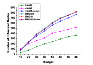
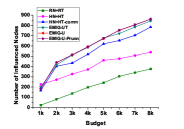
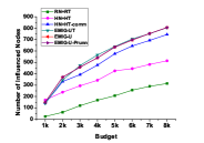
(a) Delicious (Tri)	(b) Delicious (Count)	(c) Delicious (WC)
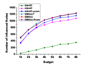
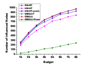
(d) Last.fm (Tri)	(e) Last.fm (Count)	(f) Last.fm (WC)
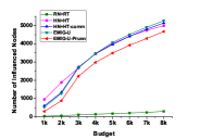
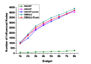
(g) LibraryThing (Tri)	(h) LibraryThing (Count)	(i) LibraryThing (WC)

Figure 2: Budget Vs. Expected Influence Plot for Delicious, Last.fm, and LibraryThing datasets under the Trivalency, Weighted Cascade and Count Probability settings.

5.3 Algorithms Compared

As the BIM Problem with tags has not been studied previously, there is no existing method with which we can compare the performance of the proposed methodologies. However, the following baseline methods have been used for comparison.

• Random Nodes and Random Tags (RN+RT): According to this method, the allocated budget is divided into two equal halves. One half will be spent for selecting seed nodes and the other one will be for selecting tags. Now seed nodes and tags are chosen randomly until their respective budgets are exhausted.

• High Degree Nodes and High Frequency Tags (HN+HT): According to this method, after dividing the budget into two equal halves, high degree nodes and high-frequency tags are chosen until their respective budget is exhausted.

• High Degree Nodes and High Frequency Tags with Communities (HN+HT+COM): In this method, after dividing the budget into two equal halves, first, the community structure of the network is detected. Both of these divided budgets are further divided among the communities based on the community size. Then apply HN+HT for each community.

All the algorithms have been implemented with Python 3.5 + NetworkX 2.1 environment on an HPC Cluster with $5$ nodes each of them having $64$ cores and $160$ GB of memory and the implementations are available at https://github.com/BITHIKA1992/BIM_with_Tag.

5.4 Goals of the Experimentation

Now, we describe the goals of the experiments:

• to make a comparative study of the proposed as well as baseline methods of their effectiveness for solving the TBIM and TEBM Problem.

• to make a comparative study of the proposed as well as baseline methods of their efficiency for solving the TBIM and TEBM Problem.

• How the value of $\alpha$ has an impact on the earned benefit?

5.5 Experimental Results with Discussions

In this section, we describe the obtained experimental results with detailed explanations. Initially, we start by describing the impact of the seed set on influence spread.

5.5.1 Impact on Influence Spread

Figure 2 shows the Budget Vs. Expected Influence plot for all the datasets under trivalency, Count, and Weighted Cascade setting. From the figures, it has been observed that the seed set selected by proposed methodologies leads to more influence compared to the baseline methods. Now, we report the dataset-wise results with examples and highlight major observations. For the ‘Delicious’ dataset, for $\mathcal{B}=8000$, under weighted cascade setting, among the baseline methods, HN+HT+COMM leads to the expected influence of $744$, whereas the same for EMIG-UT, EMIG-U, EMIG-U-Prunn methods are $804$, $805$, and $805$, respectively, which is approximately $8\%$ more compared to HN+HT+COMM. The expected influence due to the seed set selected by EMIG-U-Prunn under Weighted Cascade, trivalency, and, Count setting are $805$, $816$, and $861$ which are $62.5\%$, $63.2\%$, and $66.85\%$ of the number of nodes of the network, respectively. Also, it is important to note, that for a given budget, the number of seed nodes selected by the proposed methodologies is always more compared to baseline methods. As an example, for $\mathcal{B}=8000$, under the trivalency setting the number of seed nodes selected by RN+RT, HN+HT, and HN+HT+COMM methods are $54$. However, the same for EMIG-UT, EMIG-U, and EMIG-U-Prunn are $59$, $62$, and $62$, respectively.

In the case of ‘Last.fm’ dataset also, similar observations are made. As an example, under trivalency setting, for $\mathcal{B}=8000$, the expected influence by the proposed methodologies EMIG-UT, EMIG-U, and EMIG-U-Prunn is $1230$, $1226$, and $1219$, respectively. However, the same by RN+RT, HN+HT, and HN+HT+COMM methods are $515$, $1067$, and $1184$, respectively. In this dataset also, it has been observed that the number of seed nodes selected by the proposed methodologies is more compared to the baseline methods. As an example, under trivalency setting, for $\mathcal{B}=8000$, the number of seed nodes selected by HN+HT+COMM, and EMIG-U-Prunn are $51$ and $59$, respectively.

In this dataset, the observations are not fully consistent with the previous two datasets. It can be observed from Figure 2 ((g), (h), and (i)) that due to the pruning, the expected influence dropped significantly. As an example, in trivalency setting, for $\mathcal{B}=8000$, the expected influence by EMIG-U and EMIG-U-Prunn methods are $5265$ and $4673$, respectively. It is due to the following reason. Recall, that in the EMIG-U-Prunn methodology, we have only considered $200$ nodes for computing marginal gain in each iteration. As this dataset is larger than the previous two, hence there are many prospective nodes for which the marginal has not been computed. However, it is interesting to observe still the number of seed nodes selected by the proposed methodologies are more compared to baseline methods. Next, we describe the impact of the seed set on the earned benefit.

5.5.2 Impact on Earned Benefit

From the description in Section 5.5.1 on the influence spread, it has been observed that the computational time of EMIG-UT is excessively huge, and hence using this algorithm for seed set selection to maximize the earned benefit in real-life situations does not make much sense. Hence, in the experiments of these sections, we do not include Algorithm EMIG-UT. Also, it has been observed that in different probability settings, the number of influenced nodes does not change much, hence in this section, we perform our experiments in one (in particular ‘count probability’ setting).

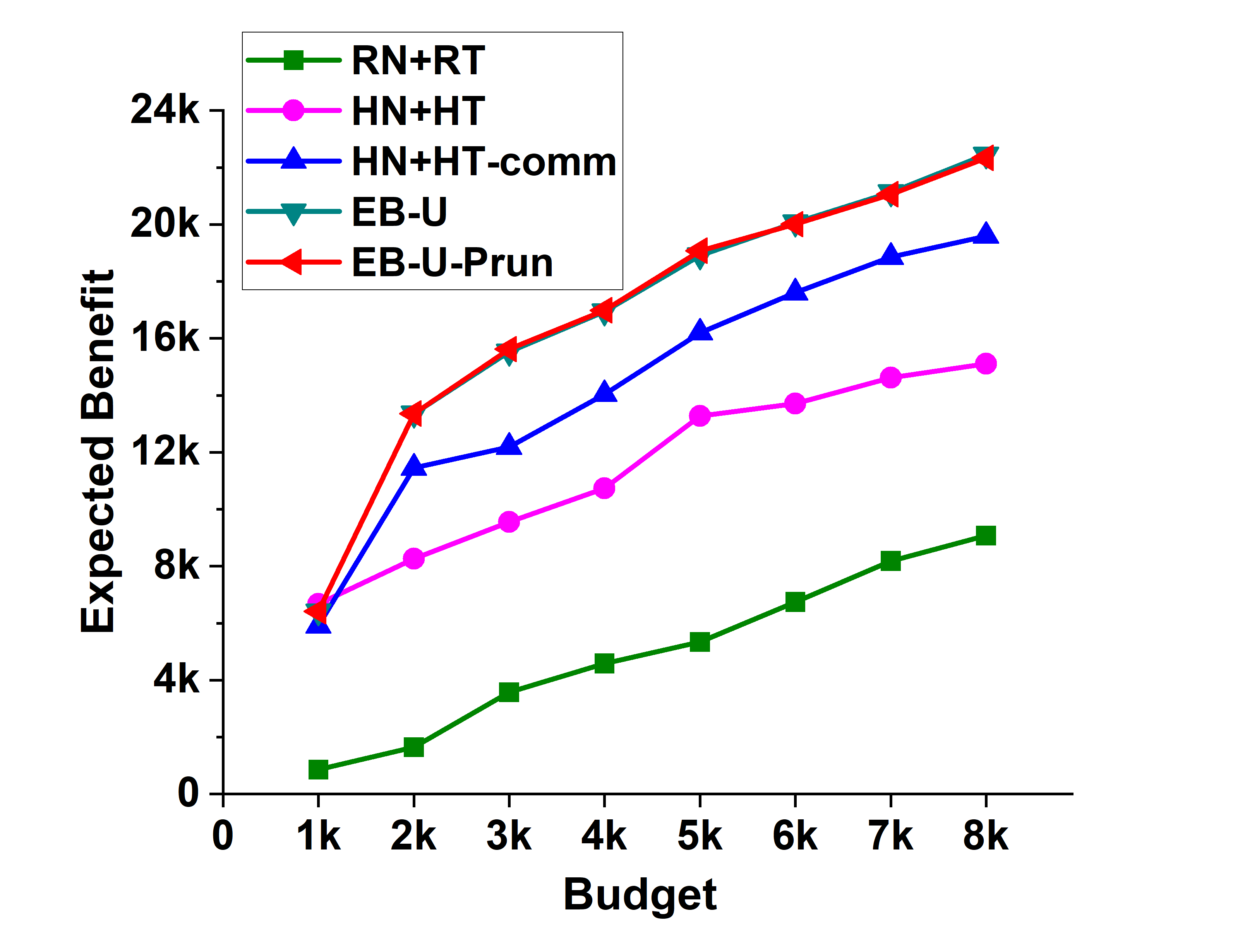
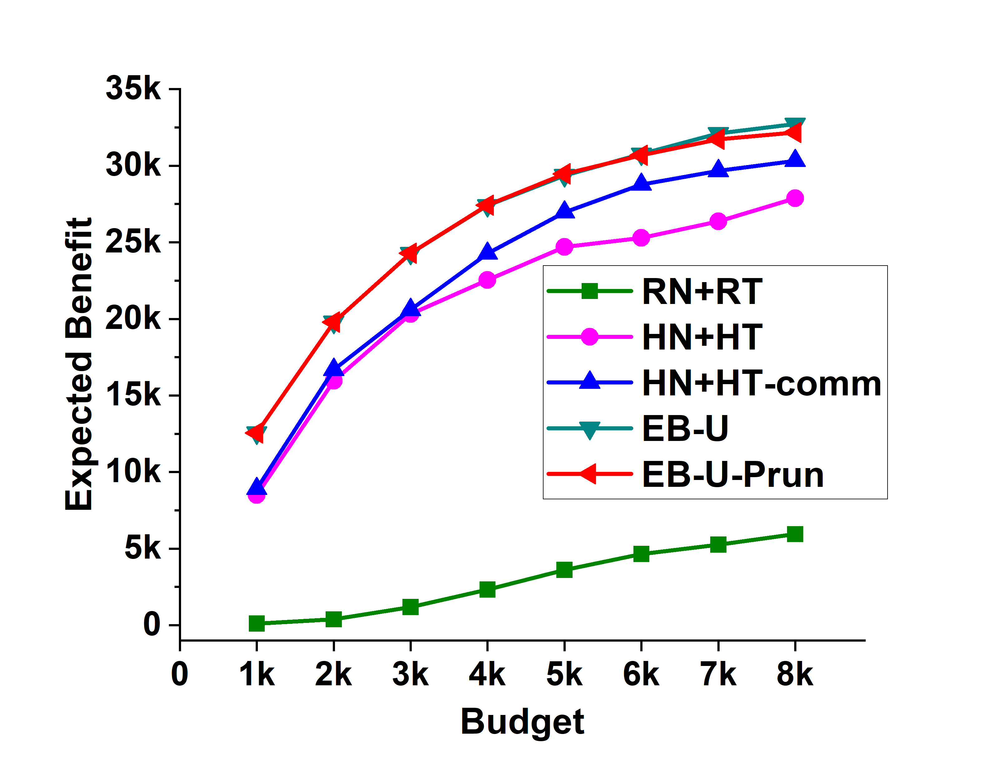
(a) Delicious	(b) Last.fm	(c) LibraryThing

Figure 3: Budget Vs. Expected Earned Benefit Plot for Delicious, Last.fm datasets under the Count Probability settings.

Figure 3 shows the plots for the Budget vs. Expected Earned Benefit Plot for all three datasets. From the figure, it has been observed that the seed set selected by the proposed methodologies leads to more amount of expected earned benefit compared to the baseline methods. As an example for the Last.fm dataset, when $\mathcal{B}=8000$, among the baseline methods the maximum amount of earned benefit was produced due to the seed sets selected by HN+HT+COMM method, and the amount is $30322$. Among the proposed methodologies EMIG-U-Prunn leads to the maximum amount of earned benefit which is $32171$ and this is $5.74\%$ more compared to the HN+HT+COMM method. It is also important to observe that for the Last.fm dataset, for $\mathcal{B}=8000$ the earned benefit due to the proposed methodologies EMIG-U and EMIG-U-Prunn are $32714$ and $32171$, respectively which is only $1.68\%$ less. However, the time requirement for EMIG-U and EMIG-U-Prunn methods are $13581$ and $6452$ seconds, respectively.

In the case of the Delicious and the LibraryThing dataset also our observations are consistent. As an example, for the Delicious dataset when $\mathcal{B}=8000$, among the baseline methods, seed set selected by the HN+HT+COMM method leads to the maximum amount of earned benefit which is $19595$. In the same setting, among the proposed methodologies the earned benefit due to the seed set selected by EMIG-U leads to the maximum amount of earned benefit which is $22449$ and this is $0.5\%$ more compared to the EMIG-U-Prunn method.

5.5.3 Impact on Computational Time

The computational time requirements for finding seed nodes by different methodologies are mentioned in Table 4. It appears that among all the methods, the RN+RT is the fastest one. HN+HT requires a little more time as it incurs the cost of computing the degree of the nodes. HN+HT+COMM requires even more time as it incurs an additional cost of detecting community structure. However, it is not observed for the ‘Delicious’ dataset as it is small in size. Among the proposed methodologies, the EMIG-UT takes the maximum execution time among all three. This is because the number of user-tag combinations in each of the datasets is excessively large and marginal gain computation in each iteration incurs huge computational time. Also, in this method, after selecting the user-tag pair in each iteration, the effective influence probability needs to be computed for all the edges after each iteration. These are the two reasons for the excessive time requirement for EMIG-UT. However, EMIG-U is taking much less time as compared to the EMIG-UT due to the less number of EMIG computations. Particularly, the ratio is of order $10$ and $10^{3}$ for the Delicious and Last.fm dataset, respectively. The proposed pruning strategy reduces the computational time even further. It is observed that the ratio between the computational time of EMIG-U and EMIG-U-Prunn for the Delicious, Last.fm, and LibraryThing are approximately $1.1$, $2$, and $10$, respectively.

Table 5 shows the computational time requirement for the seed set selection for the TEBM Problem. It is observed that among the baseline methods the RN+RT is taking the least computational time and HN+HT+Comm is taking maximum time. The reason is very simple. RN+RT method incurs the computational cost of randomly returning the nodes and tags until the budget is exhausted. On the other hand, in the case of HN+HT+Comm for all the node their degrees, for all the tags their counts in each of the communities needs to be computed and a community detection algorithm needs to be executed. Hence, the computational time for HN+HT+Comm is the highest among the baseline methods.

As mentioned previously, the main bottleneck of the proposed EMIG-U is the excessive number of EMIG computations. However, for the EMIG-U-Prunn method, as the number of EMIG computations are much less, hence this method is much faster than the EMIG-U method. In particular, this is much more visible for the Last.fm dataset. From Table 5, it can be observed that when $\mathcal{B}=8000$, the computational time requirement for selecting seed sets by EMIG-U and EMIG-U-Prunn methods are 13581.05 and 6452.45, respectively, which is approximately $2.1\%$ more.

Table 4: Computational time requirement (in Secs.) for seed set selection for the Tag-Based Budgeted Influence Maximization Problem

Dataset	Budget	Algorithm
		EMIG-U-Prunn	EMIG-U	EMIG-UT	HNHTC	HN+HT	RN+RT
Delicious	1000	130.76	182.79	$6.22\times 10^{4}$	7.86	12.78	1.01
	2000	281.72	368.97	$1.38\times 10^{4}$	10.38	13.42	2.17
	3000	404.74	523.82	$2.58\times 10^{4}$	10.67	13.22	3.60
	4000	540.40	695.64	$3.99\times 10^{4}$	10.88	14.56	5.97
	5000	704.80	866.16	$4.85\times 10^{4}$	11.33	15.26	8.27
	6000	798.86	909.35	$5.13\times 10^{4}$	11.31	13.81	11.93
	7000	926.89	1068.15	$6.92\times 10^{4}$	11.36	13.27	13.46
	8000	1085.05	1259.23	$6.82\times 10^{4}$	11.49	14.40	11.94
Last.fm	1000	305.56	712.28	$2.23\times 10^{5}$	31.37	21.05	1.85
	2000	919.89	1986.23	$8.14\times 10^{5}$	40.42	28.34	6.83
	3000	1496.92	2991.10	$1.38\times 10^{6}$	50.79	31.73	8.80
	4000	2099.94	4160.16	$1.92\times 10^{6}$	57.83	38.54	11.29
	5000	2540.25	5028.90	$2.16\times 10^{6}$	61.42	43.80	13.49
	6000	3101.83	6381.85	$2.42\times 10^{6}$	67.92	47.37	16.74
	7000	3613.09	7248.25	$2.74\times 10^{6}$	69.97	50.62	20.89
	8000	4032.52	7954.09	$2.91\times 10^{6}$	70.32	50.99	22.40
Library	1000	1792.85	$2.52\times 10^{4}$	N.A.	134.20	89.95	174.40
	2000	4870.87	$6.35\times 10^{4}$	N.A.	222.54	129.36	234.08
	3000	9328.23	$1.17\times 10^{5}$	N.A.	241.19	170.45	265.36
	4000	13193.17	$1.65\times 10^{5}$	N.A.	288.62	185.27	308.76
	5000	17242.24	$2.03\times 10^{5}$	N.A.	312.22	218.72	342.88
	6000	21705.09	$2.48\times 10^{5}$	N.A.	331.24	232.68	344.22
	7000	25269.24	$2.84\times 10^{5}$	N.A.	365.39	264.74	379.19
	8000	29544.79	$3.26\times 10^{5}$	N.A.	390.14	264.54	386.04

Table 5: Computational time requirement (in Secs.) for seed set selection for the Tag-Based Earned Benefit Maximization Problem

Dataset	Budget	Algorithm
		EMIG-U-Prunn	EMIG-U	HNHTC	HN+HT	RN+RT
Delicious	1000	174.10	243.60	7.40	7.76	1.64
	2000	447.12	622.62	10.18	9.809	3.31
	3000	624.97	873.46	10.44	10.69	6.35
	4000	831.82	1442.17	11.26	10.71	7.40
	5000	1020.15	1275.10	11.29	11.19	8.19
	6000	1335.74	1571.07	11.52	11.27	8.39
	7000	1505.23	1788.42	11.64	11.66	9.34
	8000	1630.12	1952.08	11.87	11.69	9.65
Last.fm	1000	456.09	1199.66	24.65	23.74	1.37
	2000	1227.08	2854.29	33.30	33.06	3.19
	3000	2029.02	4661.47	40.61	37.31	4.01
	4000	2920.05	6311.78	49.87	44.96	4.68
	5000	3806.55	8099.59	54.22	50.03	10.43
	6000	4527.61	9695.24	56.99	53.24	11.95
	7000	5413.39	11620.07	58.01	59.76	15.20
	8000	6452.45	13581.05	61.72	58.80	15.70

5.5.4 Impact of $\alpha$

In this section, we describe the impact of $\alpha$ on the earned benefit. From Equation 12, it is easy to understand that $\alpha$ tries to balance between the cost of the nodes in a community with their corresponding benefits, to prioritize the budget allocation for a community. If $\alpha=1$, only the cost of the nodes contributes to the budget allocation, whereas in the case of $\alpha=0$, the benefits of the users are considered. For both delicious and last.fm datasets, the results of expected earned benefit for different $\alpha(e.g.,0.0,0.25,0.5,0.75,1.0)$ values are shown in Figure 4. The cost of the users is chosen uniformly at random within the range of 50 to 100. The benefit is also selected within the same range of cost, and it returns zero if neither the user nor his neighbor selects at least one targeted tag. For all the methods which use community-based budget allocation, the change in expected benefits are visible for smaller values of budget and it is maximum for $\alpha=zero$. Compared to HN+HT-Comm, the expected benefit-based algorithms are more uniform for different values of $\alpha$, due to their uniform choice of cost and benefits range. One interesting point to notice here is that in both the datasets, the earned benefit gaps within HN+HT-Comm and expected-benefit based algorithms are high for large value of $\alpha$, i.e., when the budget is almost dependent on the cost of users, the high degree node does not incur the maximum expected benefit.

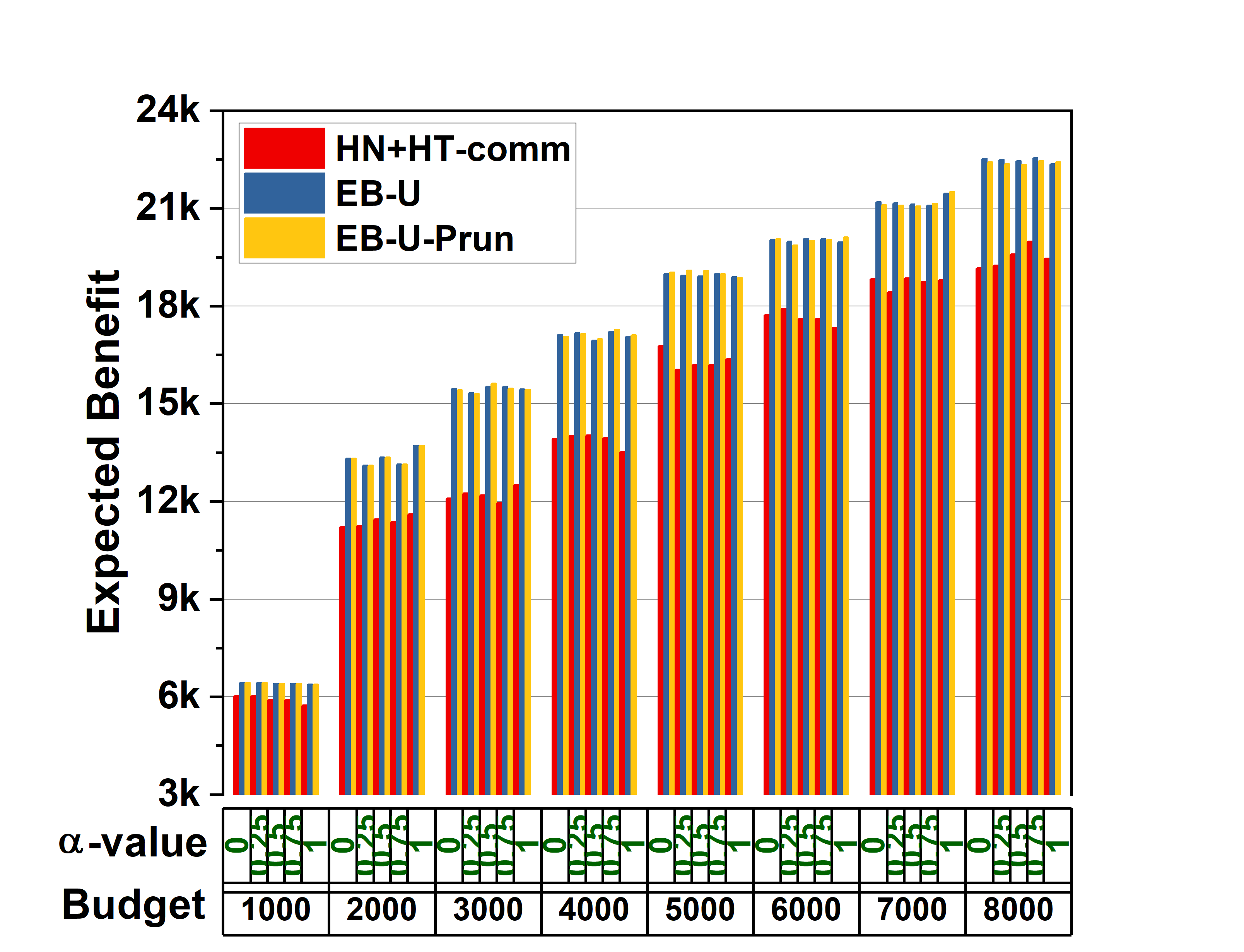
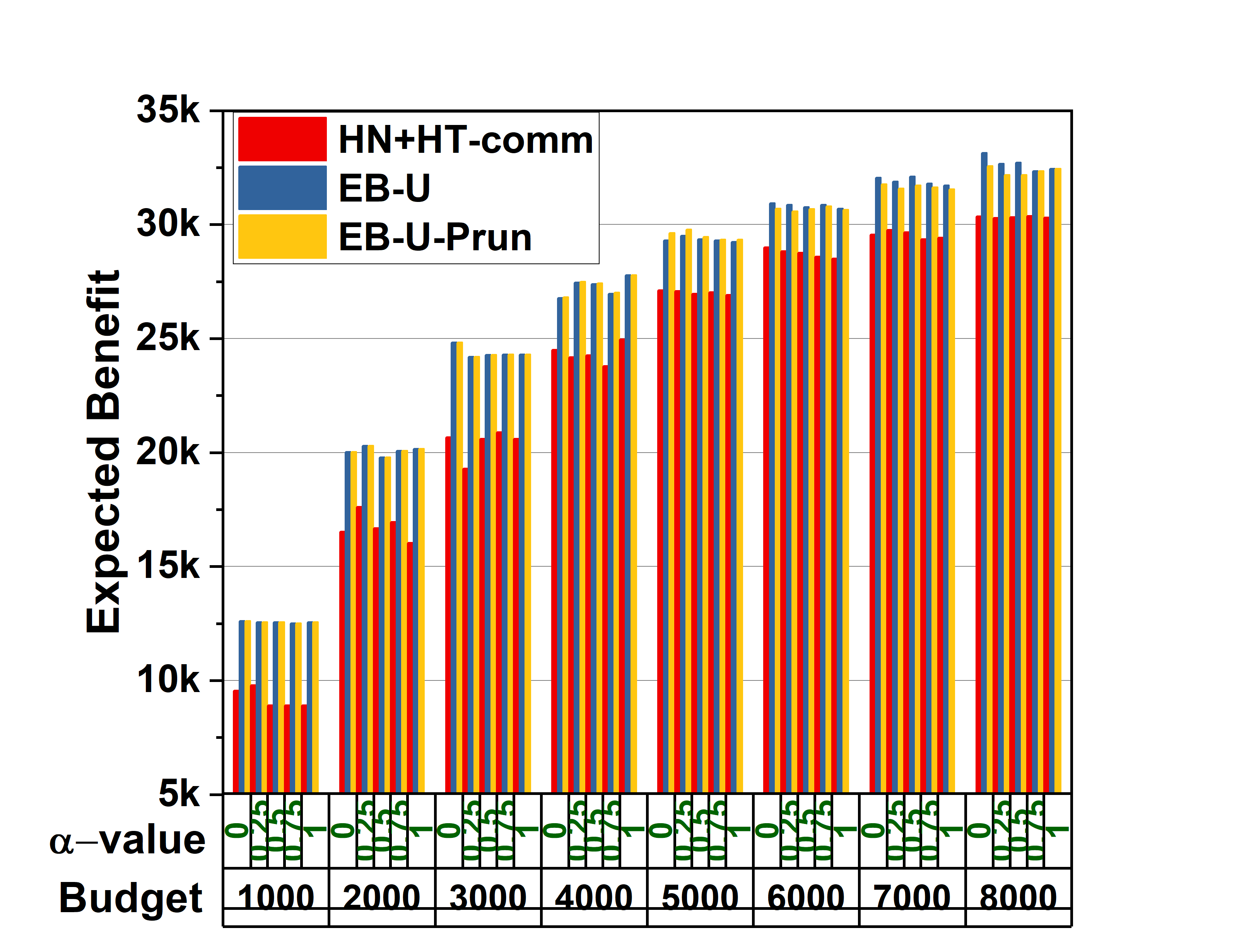
(a) Delicious	(b) Last.fm

Figure 4: Impact of $\alpha$ on Earned Benefit on Delicious and Last.fm Dataset

6 Conclusion

In this paper, we have introduced the Tag-Based Budgeted Influence Maximization Problem and the Tag-Based Earned Benefit Maximization Problem. For both these problems, considering the ground truth that different tags have a different level of popularity in different communities, three different methodologies have been proposed. All the methodologies have been analyzed for their time and space requirements. From the experimental results, it has been observed that the seed set selected by the proposed methodologies leads to better influence spread compared to the baseline methods. Our future study on this problem will remain concentrated on developing efficient pruning techniques, which reduces the computational time without affecting the influence spread much. A number of avenues are open to extend this work. In this study, we have not considered the presence of negative information spreader. Our study can be enhanced by considering this situation. Also, efficient pruning techniques can be proposed such that the proposed methodologies will be much more efficient.

References

- Banerjee et al. [2019a] Banerjee, S., Jenamani, M., Pratihar, D.K., 2019a. Combim: A community-based solution approach for the budgeted influence maximization problem. Expert Systems with Applications .
- Banerjee et al. [2019b] Banerjee, S., Jenamani, M., Pratihar, D.K., 2019b. Maximizing the earned benefit in an incentivized social networking environment: a community-based approach. Journal of Ambient Intelligence and Humanized Computing , 1–17.
- Banerjee et al. [2019c] Banerjee, S., Jenamani, M., Pratihar, D.K., 2019c. Maximizing the earned benefit in an incentivized social networking environment: An integer programming-based approach, in: Proceedings of the ACM India Joint International Conference on Data Science and Management of Data, pp. 322–325.
- Banerjee et al. [2020a] Banerjee, S., Jenamani, M., Pratihar, D.K., 2020a. Earned benefit maximization in social networks under budget constraint. Expert Systems with Applications , 114346.
- Banerjee et al. [2020b] Banerjee, S., Jenamani, M., Pratihar, D.K., 2020b. A survey on influence maximization in a social network. Knowledge and Information Systems , 1–39.
- Banerjee et al. [2020c] Banerjee, S., Pal, B., Jenamani, M., 2020c. Budgeted influence maximization with tags in social networks, in: International Conference on Web Information Systems Engineering, Springer. pp. 141–152.
- Bozorgi et al. [2016] Bozorgi, A., Haghighi, H., Zahedi, M.S., Rezvani, M., 2016. Incim: A community-based algorithm for influence maximization problem under the linear threshold model. Information Processing & Management 52, 1188–1199.
- Bozorgi et al. [2017] Bozorgi, A., Samet, S., Kwisthout, J., Wareham, T., 2017. Community-based influence maximization in social networks under a competitive linear threshold model. Knowledge-Based Systems 134, 149–158.
- Buchbinder et al. [2015] Buchbinder, N., Feldman, M., Seffi, J., Schwartz, R., 2015. A tight linear time (1/2)-approximation for unconstrained submodular maximization. SIAM Journal on Computing 44, 1384–1402.
- Bucur and Iacca [2016] Bucur, D., Iacca, G., 2016. Influence maximization in social networks with genetic algorithms, in: European Conference on the Applications of Evolutionary Computation, Springer. pp. 379–392.
- Cai et al. [2017] Cai, C., He, R., McAuley, J., 2017. Spmc: socially-aware personalized markov chains for sparse sequential recommendation. arXiv preprint arXiv:1708.04497 .
- Cantador et al. [2011] Cantador, I., Brusilovsky, P., Kuflik, T., 2011. 2nd workshop on information heterogeneity and fusion in recommender systems (hetrec 2011), in: Proceedings of the 5th ACM conference on Recommender systems, ACM, New York, NY, USA.
- Carrington et al. [2005] Carrington, P.J., Scott, J., Wasserman, S., 2005. Models and methods in social network analysis. volume 28. Cambridge university press.
- Chen et al. [2011] Chen, W., Collins, A., Cummings, R., Ke, T., Liu, Z., Rincon, D., Sun, X., Wang, Y., Wei, W., Yuan, Y., 2011. Influence maximization in social networks when negative opinions may emerge and propagate, in: Proceedings of the 2011 siam international conference on data mining, SIAM. pp. 379–390.
- Chen et al. [2010] Chen, W., Wang, C., Wang, Y., 2010. Scalable influence maximization for prevalent viral marketing in large-scale social networks, in: Proceedings of the 16th ACM SIGKDD international conference on Knowledge discovery and data mining, ACM. pp. 1029–1038.
- Chen et al. [2012] Chen, Y., Chang, S., Chou, C., Peng, W., Lee, S., 2012. Exploring community structures for influence maximization in social networks, in: The 6th SNA-KDD Workshop on Social Network Mining and Analysis Held in Conjunction with KDD, pp. 1–6.
- Chen et al. [2014] Chen, Y.C., Zhu, W.Y., Peng, W.C., Lee, W.C., Lee, S.Y., 2014. Cim: Community-based influence maximization in social networks. ACM Transactions on Intelligent Systems and Technology (TIST) 5, 25.
- Domingos and Richardson [2001] Domingos, P., Richardson, M., 2001. Mining the network value of customers, in: Proceedings of the seventh ACM SIGKDD international conference on Knowledge discovery and data mining, ACM. pp. 57–66.
- Fan et al. [2018] Fan, J., Qiu, J., Li, Y., Meng, Q., Zhang, D., Li, G., Tan, K.L., Du, X., 2018. Octopus: An online topic-aware influence analysis system for social networks, in: 2018 IEEE 34th International Conference on Data Engineering (ICDE), IEEE. pp. 1569–1572.
- Feige et al. [2011] Feige, U., Mirrokni, V.S., Vondrák, J., 2011. Maximizing non-monotone submodular functions. SIAM Journal on Computing 40, 1133–1153.
- Galhotra et al. [2015] Galhotra, S., Arora, A., Virinchi, S., Roy, S., 2015. Asim: A scalable algorithm for influence maximization under the independent cascade model, in: Proceedings of the 24th International Conference on World Wide Web, ACM. pp. 35–36.
- Gong et al. [2016] Gong, M., Yan, J., Shen, B., Ma, L., Cai, Q., 2016. Influence maximization in social networks based on discrete particle swarm optimization. Information Sciences 367, 600–614.
- Goyal et al. [2011] Goyal, A., Lu, W., Lakshmanan, L.V., 2011. Celf++: optimizing the greedy algorithm for influence maximization in social networks, in: Proceedings of the 20th international conference companion on World wide web, ACM. pp. 47–48.
- Güney [2017] Güney, E., 2017. On the optimal solution of budgeted influence maximization problem in social networks. Operational Research , 1–15.
- Han et al. [2014] Han, S., Zhuang, F., He, Q., Shi, Z., 2014. Balanced seed selection for budgeted influence maximization in social networks, in: Pacific-Asia Conference on Knowledge Discovery and Data Mining, Springer. pp. 65–77.
- Hosseini-Pozveh et al. [2017] Hosseini-Pozveh, M., Zamanifar, K., Naghsh-Nilchi, A.R., 2017. A community-based approach to identify the most influential nodes in social networks. Journal of Information Science 43, 204–220.
- Huang et al. [2019] Huang, H., Shen, H., Meng, Z., Chang, H., He, H., 2019. Community-based influence maximization for viral marketing. Applied Intelligence , 1–14.
- Huang et al. [2020] Huang, K., Tang, J., Xiao, X., Sun, A., Lim, A., 2020. Efficient approximation algorithms for adaptive target profit maximization, in: 2020 IEEE 36th International Conference on Data Engineering (ICDE), IEEE. pp. 649–660.
- Ienco et al. [2010] Ienco, D., Bonchi, F., Castillo, C., 2010. The meme ranking problem: Maximizing microblogging virality, in: 2010 IEEE International Conference on Data Mining Workshops, IEEE. pp. 328–335.
- Ke et al. [2018] Ke, X., Khan, A., Cong, G., 2018. Finding seeds and relevant tags jointly: For targeted influence maximization in social networks, in: Proceedings of the 2018 International Conference on Management of Data, ACM. pp. 1097–1111.
- Kempe et al. [2003] Kempe, D., Kleinberg, J., Tardos, É., 2003. Maximizing the spread of influence through a social network, in: Proceedings of the ninth ACM SIGKDD international conference on Knowledge discovery and data mining, ACM. pp. 137–146.
- Leskovec et al. [2007] Leskovec, J., Krause, A., Guestrin, C., Faloutsos, C., VanBriesen, J., Glance, N., 2007. Cost-effective outbreak detection in networks, in: Proceedings of the 13th ACM SIGKDD international conference on Knowledge discovery and data mining, ACM. pp. 420–429.
- Li et al. [2018a] Li, X., Cheng, X., Su, S., Sun, C., 2018a. Community-based seeds selection algorithm for location aware influence maximization. Neurocomputing 275, 1601–1613.
- Li et al. [2018b] Li, Y., Fan, J., Wang, Y., Tan, K.L., 2018b. Influence maximization on social graphs: A survey. IEEE Transactions on Knowledge and Data Engineering 30, 1852–1872.
- Li et al. [2015] Li, Y., Zhang, D., Tan, K.L., 2015. Real-time targeted influence maximization for online advertisements. Proceedings of the VLDB Endowment 8, 1070–1081.
- Liu et al. [2020] Liu, B., Li, X., Wang, H., Fang, Q., Dong, J., Wu, W., 2020. Profit maximization problem with coupons in social networks. Theoretical Computer Science 803, 22–35.
- Narayanam and Narahari [2011] Narayanam, R., Narahari, Y., 2011. A shapley value-based approach to discover influential nodes in social networks. IEEE Transactions on Automation Science and Engineering 8, 130–147.
- Nguyen and Zheng [2013] Nguyen, H., Zheng, R., 2013. On budgeted influence maximization in social networks. IEEE Journal on Selected Areas in Communications 31, 1084–1094.
- Peng et al. [2018] Peng, S., Zhou, Y., Cao, L., Yu, S., Niu, J., Jia, W., 2018. Influence analysis in social networks: A survey. Journal of Network and Computer Applications 106, 17–32.
- Shang et al. [2017] Shang, J., Zhou, S., Li, X., Liu, L., Wu, H., 2017. Cofim: A community-based framework for influence maximization on large-scale networks. Knowledge-Based Systems 117, 88–100.
- Singh et al. [2019] Singh, S.S., Kumar, A., Singh, K., Biswas, B., 2019. C2im: Community based context-aware influence maximization in social networks. Physica A: Statistical Mechanics and its Applications 514, 796–818.
- Tang et al. [2017] Tang, J., Tang, X., Yuan, J., 2017. Profit maximization for viral marketing in online social networks: Algorithms and analysis. IEEE Transactions on Knowledge and Data Engineering 30, 1095–1108.
- Tang et al. [2015] Tang, Y., Shi, Y., Xiao, X., 2015. Influence maximization in near-linear time: A martingale approach, in: Proceedings of the 2015 ACM SIGMOD International Conference on Management of Data, ACM. pp. 1539–1554.
- Tang et al. [2014] Tang, Y., Xiao, X., Shi, Y., 2014. Influence maximization: Near-optimal time complexity meets practical efficiency, in: Proceedings of the 2014 ACM SIGMOD international conference on Management of data, ACM. pp. 75–86.
- Tong et al. [2018] Tong, G., Wu, W., Du, D.Z., 2018. Coupon advertising in online social systems: Algorithms and sampling techniques. arXiv preprint arXiv:1802.06946 .
- Wang et al. [2012] Wang, C., Chen, W., Wang, Y., 2012. Scalable influence maximization for independent cascade model in large-scale social networks. Data Mining and Knowledge Discovery 25, 545–576.
- Wang et al. [2010] Wang, Y., Cong, G., Song, G., Xie, K., 2010. Community-based greedy algorithm for mining top-k influential nodes in mobile social networks, in: Proceedings of the 16th ACM SIGKDD international conference on Knowledge discovery and data mining, ACM. pp. 1039–1048.
- Zhang et al. [2013] Zhang, J., Wang, Y., Vassileva, J., 2013. Socconnect: A personalized social network aggregator and recommender. Information Processing & Management 49, 721–737.
- Zhang et al. [2017] Zhang, K., Du, H., Feldman, M.W., 2017. Maximizing influence in a social network: Improved results using a genetic algorithm. Physica A: Statistical Mechanics and its Applications 478, 20–30.
- Zhao et al. [2015] Zhao, T., McAuley, J., King, I., 2015. Improving latent factor models via personalized feature projection for one class recommendation, in: Proceedings of the 24th ACM international on conference on information and knowledge management, ACM. pp. 821–830.
- Zhou et al. [2019] Zhou, J., Fan, J., Wang, J., Wang, X., Li, L., 2019. Cost-efficient viral marketing in online social networks. World Wide Web 22, 2355–2378.
- Zhu et al. [2017] Zhu, Y., Li, D., Yan, R., Wu, W., Bi, Y., 2017. Maximizing the influence and profit in social networks. IEEE Transactions on Computational Social Systems 4, 54–64.