Regularized Maximum Likelihood Estimation for the Random Coefficients Model

Abstract

The random coefficients model $Y_{i}={\beta_{0}}_{i}+{\beta_{1}}_{i}{X_{1}}_{i}+{\beta_{2}}_{i}{X_{2}}_{i}+\ldots+{\beta_{d}}_{i}{X_{d}}_{i}$, with $\mathbf{X}_{i}$, $Y_{i}$, ${\bm{\beta}}_{i}$ i.i.d, and ${\bm{\beta}}_{i}$ independent of $\mathbf{X}_{i}$ is often used to capture unobserved heterogeneity in a population. We propose a quasi-maximum likelihood method to estimate the joint density distribution of the random coefficient model. This method implicitly involves the inversion of the Radon transformation in order to reconstruct the joint distribution, and hence is an inverse problem. Nonparametric estimation for the joint density of ${\bm{\beta}}_{i}=({\beta_{0}}_{i},\ldots,{\beta_{d}}_{i})$ based on kernel methods or Fourier inversion have been proposed in recent years. Most of these methods assume a heavy tailed design density $f_{\mathbf{X}}$. To add stability to the solution, we apply regularization methods. We analyze the convergence of the method without assuming heavy tails for $f_{\mathbf{X}}$ and illustrate performance by applying the method on simulated and real data. To add stability to the solution, we apply a Tikhonov-type regularization method.

1 Introduction

Unobserved heterogeneity in a population is an important problem in statistics and econometrics. A common way to account for unobserved heterogeneity is the use of random effects or mixed models which usually impose parametric assumptions on the distribution of the random effects. This is a significant restriction on the structure of the heterogeneity. In recent years the linear random coefficient model, which is a nonparametric alternative, attracted significant attention in the literature. This model is given by

$$Y_{i}=\beta_{0i}+\beta_{1i}X_{1i}+\beta_{2i}X_{2i}+\ldots+\beta_{di}X_{di}.$$ (1)

With ${\bm{\beta}}_{i}=(\beta_{0i},\beta_{1i},\beta_{2i},\ldots,\beta_{di})^{\top}$ and $\mathbf{X}_{i}=(1,X_{1i},X_{2i},\ldots X_{di})^{\top}$ we can write (1) as $Y_{i}={\bm{\beta}}_{i}^{\top}\mathbf{X}_{i}$. We assume that $\mathbf{X}_{i}$, $Y_{i}$, ${\bm{\beta}}_{i}$ are i.i.d random variables with ${\bm{\beta}}_{i}$ and $\mathbf{X}_{i}$ being independent, and that $Y_{i}$ and $\mathbf{X}_{i}$ are observed while ${\bm{\beta}}_{i}$ is unknown. The objective is to estimate the joint density $f_{\bm{\beta}}$ of ${\bm{\beta}}_{i}$ nonparametrically.

In this paper we propose and analyze a regularized maximum likelihood estimator for the density $f_{\bm{\beta}}$

$$\hat{f}_{\bm{\beta}}=\operatorname*{arg\,min}_{f\geq 0,\,\|f\|_{L^{1}}=1}-\ell(f|Y_{1},\mathbf{X}_{1},\ldots Y_{n},\mathbf{X}_{n})+\alpha\mathcal{R}(f)$$ (2)

Here $\ell$ is the log-likelihood functional, $\alpha\geq 0$ is a smoothing parameter, and $\mathcal{R}$ is a convex lower semi-continuous functional which regularizes the estimator. Both $\alpha$ and $\mathcal{R}$ are chosen by the statistician. The choice of $\mathcal{R}$ can consider a priori information about $f_{\bm{\beta}}$ like smoothness or sparsity. Details of the method and examples for $\mathcal{R}$ will be presented in Section 2. Estimating $f_{\bm{\beta}}$ from observations of $Y_{i}$ and $\mathbf{X}_{i}$ is an ill-posed inverse problem. The degree of ill-posedness depends on the tail behavior of the design density $f_{\mathbf{X}}$.

In this paper we give conditions for method (2) to achieve the optimal rates for design densities with different tail behavior or with bounded support. We evaluate the the small sample performance in simulations and have a data application in consumer demand.

Nonparametric estimation in model (1) with one regressor, i.e. $d=1$ was first developed by Beran and Hall, (1992); Beran et al., (1996); Feuerverger and Vardi, (2000). The optimal rate for design densities with Cauchy-type tails is derived in Hoderlein et al., (2010) for a kernel method. For the special case of just one regressor, i.e. $d=1$, optimal rates for tails with polynomial decay are presented in Holzmann and Meister, (2020). Faster decay of the tails and even bounded support for one regressor was considered in Hohmann and Holzmann, (2016). Testing in model (1) has been considered in Breunig and Hoderlein, (2018); Dunker et al., (2019).

Regularized maximum likelihood methods have been considered for other problems than model (1), e.g. in Werner and Hohage, (2012); Hohage and Werner, (2013, 2016); Dunker and Hohage, (2014). We also refer to the literature on general convex regularization functionals, see Scherzer et al., (2009); Schuster et al., (2012); Benning and Burger, (2018) for an overview.

Random coefficients modmodels are frequently used to evaluate panel data, cf. Hsiao, (2014) or Hsiao and Pesaran, (2004), Chapter 6, for an overview. Modeling and estimating consumer demand in industrial organization and marketing often makes use of random coefficients Berry et al., (1995); Petrin, (2002); Nevo, (2001); Dubé et al., (2012). In all these works, parametric assumptions on $f_{{\bm{\beta}}}$ are imposed. els are applied in econometrics, epidemiology, and quantum mechanics. Applications in epidemiology are considered by Greenland, (2000); Gustafson and Greenland, (2006). In economics, random coefficients Recently, nonparametric approaches for random coefficients became popular in microeconometrics Hoderlein et al., (2010); Masten, (2018); Hoderlein et al., (2017), frequently combined with binary choice Ichimura and Thompson, (1998); Berry and Pakes, (2007); Gautier and Hoderlein, (2012); Gautier and Kitamura, (2013); Masten and Torgovitsky, (2016); Dunker et al., (2013); Fox and Gandhi, (2016); Dunker et al., (2017, 2018), among others. The random coefficients model also appears in quantum homodyne tomography, see Feuerverger and Vardi, (2000); Butucea et al., (2007).

The paper is organized as follows. Section 2 gives a detailed account of the method. A convergence rate result is presented in Section 3. We explain our implementation of the method in Section 4 and show simulation results in Section 5. Section 6 presents an application to real data. The paper closes with a conclusion in Section 7.

2 Method

Throughout this paper we assume that ${\bm{\beta}}$ has a Lebesgue density $f_{\bm{\beta}}$. If in addition the conditional density $f_{Y|\mathbf{X}}$ exists, the two densities are connected by the integral equation

$$f_{Y|\mathbf{X}}(y|\mathbf{X}=\mathbf{x})=\int_{\mathbbm{R}^{d}}\mathbbm{1}\big{\{}\mathbf{b}^{\top}\mathbf{x}=y\big{\}}f_{\bm{\beta}}(\mathbf{b})d\mu_{d}(\mathbf{b})=\int_{\mathbf{b}^{\top}\mathbf{x}=y}f_{\bm{\beta}}(\mathbf{b})d\mu_{d}(\mathbf{b})$$ (3)

where $\mathbbm{1}$ denotes the index function and $\mu_{d}$ the induced Lebesgue measure on the $d$-dimensional hyper-plane given by $\mathbf{b}^{\top}\mathbf{X}=Y$. It was pointed out in Beran et al., (1996) that (3) becomes the well known Radon transformation $f_{S|{\bm{\Theta}}}=\mathcal{R}(f_{\bm{\beta}})$ when $\mathbf{X}$ and $Y$ are normalized to ${\bm{\Theta}}=\mathbf{X}/\|\mathbf{X}\|$ and $S=Y/\|\mathbf{X}\|$. The injectivity of the Randon transformation implies that $f_{\bm{\beta}}$ is identified when the support of ${\bm{\Theta}}$ contains an open neighborhood, see Masten, (2018) for minimal conditions.

It is well known that an integral equation of the first kind like (3) and the Radon transformation are ill-posed inverse problems, i.e. $f_{\bm{\beta}}$ does not depend continuously on $f_{Y|\mathbf{X}}$ or $f_{S|{\bm{\Theta}}}$. Nonparametric estimation of $f_{\bm{\beta}}$ requires regularization. It is possible to derive a nonparametric estimate for $f_{\bm{\beta}}$ by inverting the Radon transformation on a nonparametric estimator $\hat{f}_{S|{\bm{\Theta}}}$. We want to avoid this two step approach and suggest an estimator that allows the statistician to use a priori knowledge of $f_{\bm{\beta}}$ if available.

Our method is based on maximum likelihood estimation. The likelihood functional for $f_{\bm{\beta}}$ given the observations is

$$\mathcal{L}(f_{\bm{\beta}}|Y,\mathbf{X})=\prod_{i=1}^{n}\int_{\mathbbm{R}}\mathbbm{1}\big{\{}{\bm{\beta}}_{i}^{\top}\mathbf{X}_{i}=Y_{i}\big{\}}f_{\bm{\beta}}(\mathbf{b})d\mu(\mathbf{b}),$$ (4)

which leads to the expression for the average log-likelihood

$$\bar{\ell}(f_{\bm{\beta}}|Y,\mathbf{X})=\frac{1}{n}\sum_{i=1}^{n}\log\left[\int_{\mathbbm{R}}\mathbbm{1}\big{\{}{\bm{\beta}}_{i}^{\top}\mathbf{X}_{i}=Y_{i}\big{\}}f_{\bm{\beta}}(b)d\mu(\mathbf{b})\right].$$ (5)

Direct maximization of $\bar{\ell}(f_{\bm{\beta}}|Y,\mathbf{X})$ over all densities it not feasible due to ill-posedness and will lead to overfitting. We stabilize the problem by adding a penalty term $\alpha\mathcal{R}(f_{\bm{\beta}})$ and state the estimator as a minimization problem with negative log-likelihood

$$\hat{f_{\bm{\beta}}}_{\alpha}=\operatorname*{arg\,min}_{f\geq 0,\,\|f\|_{L^{1}}=1}-\bar{\ell}(f|Y,\mathbf{X})+\alpha\mathcal{R}(f).$$ (6)

Here $\alpha\geq 0$ is a regularization parameter that controls a bias variance trade-off. Furthermore, $\mathcal{R}$ is a convex lower semi-continuous functional. Typical choices for $\mathcal{R}$ are

• Squared $L^{2}$ norm: $\mathcal{R}(f)=\|f\|_{L^{2}}^{2}=\|f\|_{2}^{2}$.

• Sobolev Norm for $H^{r}$: $\mathcal{R}(f)=\|f_{\beta}\|_{2}^{2}+\|f^{\prime}_{\beta}\|_{2}^{2}+\ldots+\|f^{(r)}_{\beta}\|_{2}^{2}$.

• $L^{p}$ norm: $\mathcal{R}(f)=\|f\|_{L^{p}}^{p}=\|f\|_{p}^{p}$ with $0\leq p\leq\infty$.

• Sobolev Norm for $W^{r}_{p}$: $\mathcal{R}(f)=\|f_{\beta}\|_{p}^{p}+\|f^{\prime}_{\beta}\|_{p}^{p}+\ldots+\|f^{(r)}_{\beta}\|_{p}^{p}$.

• Entropy: $\mathcal{R}(f)=\int{f(\mathbf{b})\ln{f(\mathbf{b})}d\mathbf{b}}$.

While an $L^{p}$ penalty implies that the estimator $\hat{f}_{\bm{\beta}}$ is in $L^{p}$, a Sobolev norm enforces more smoothness on the estimator. Note that an entropy penalty is natural for estimating a density. It does not imply that $f_{\bm{\beta}}$ belongs to a particular $L^{p}$ space other than $L^{1}$ and only enforces a finite entropy. If a priori knowledge about $f_{\bm{\beta}}$ like smoothness is available, $\mathcal{R}$ can be chosen accordingly.

In addition to the regularization functional the regularization parameter $\alpha$ needs to be chosen. As usual in nonparametric estimation the optimal $\alpha$ depends on the unknown $f_{\bm{\beta}}$. We propose adaptive estimation by Lepskii’s principle which is popular for inverse problems, e.g. Tsybakov, (2000), Bauer and Hohage, (2005), Mathé, (2006), Hohage and Werner, (2016), Werner, (2018), and Holzmann and Meister, (2020). It is computationally cheaper than many other parameter selection rules like cross-validation, which is a big advantage since our problem is already computationally demanding.

The principle works as follows: we compute the estimator $\hat{f}_{{\bm{\beta}}_{\alpha_{1}}},\ldots,\hat{f}_{{\bm{\beta}}_{\alpha_{m}}}$ for several parameters $\alpha_{1}<\alpha_{1}<\ldots<\alpha_{m}$ together with a bound on the standard deviation of each estimator which is a non-increasing function $\Psi:\{i,\ldots,m\}\rightarrow\mathbbm{R}$ which is specified in Theorem 5. The Lepskii regularization parameter $\alpha_{\bar{j}}$ is selected by

$$\bar{j}:=\max\{j\leq m,\|{f_{\bm{\beta}}}_{\alpha_{i}},{f_{\bm{\beta}}}_{\alpha_{j}}\|\leq 2\Psi(i),\text{ for all }i\leq j\}.$$

For further details on this parameter choice we refer to Lepskiĭ, (1991),Mathé, (2006), and Hohage and Werner, (2016).

Our method can be interpreted as an elastic net with $L^{1}$ penalty combined with the penalty term given by $\mathcal{R}$. It was poined out in Heiss et al., (2019) that the constraint $\|f_{\bm{\beta}}\|_{L^{1}}=1$ together with a finite difference discretization of $f_{\bm{\beta}}$ is equivalent to an $\ell^{1}$ penalty on the discretized values of $f_{\bm{\beta}}$. Without the additional penalty term $\alpha\mathcal{R}(f_{\bm{\beta}})$ this would lead to an unwanted shrinkage in the estimate which would set $\hat{f}_{\bm{\beta}}$ to $0$ at most grid points and produce relatively large values for $\hat{f}_{\bm{\beta}}$ at only a few grid points. To reduce this LASSO-type effect Heiss et al., (2019) introduce an additional quadratic constraint which transforms the method into an elastic net. This is analogous to our regularization term $\alpha\mathcal{R}(f_{\bm{\beta}})$ although our setup is more flexible since it allows for a wide range of regularization functionals and not only for quadratic $\mathcal{R}$.

3 Convergence rates

In this section we establish some theoretical properties of the estimator, such as the existence, and uniqueness of the solution to (6), as well as its convergence properties. For technical reasons, we will state the theory for the normalized variables ${\bm{\Theta}}=\mathbf{X}/\|\mathbf{X}\|$ and $S=Y/\|\mathbf{X}\|$. Note that the estimator $\hat{f}_{\bm{\beta}}$ in (6) does not change when we replace $\mathbf{X}$ by ${\bm{\Theta}}$ and $Y$ by $S$.

3.1 Assumptions

We define the linear compact integral operator

$$(Tf)({\bm{\theta}},s)=\int_{\mathbbm{R}^{d}}\mathbbm{1}\big{\{}\mathbf{b}^{\top}{\bm{\theta}}=s\big{\}}f(\mathbf{b})d\mu_{d}(\mathbf{b}).$$

Hence, we are solving the inverse ill-posed problem

$$f_{S|{\bm{\Theta}}}=Tf_{\beta}.$$ (7)

We start by discussing the assumptions.

Assumption 1.

We have i.i.d. samples $S_{i},{\bm{\Theta}}_{i}$, $i=1,\ldots,n$ generated by model (1) with independent ${\bm{\beta}}_{i}$ and ${\bm{\Theta}}_{i}$. Let $B\subset L^{1}(\mathbbm{R}^{d+1})$ be convex with $f_{\bm{\beta}}\in B$ and $T:B\rightarrow H^{s}(D)$ where $H^{s}$ is an $L^{2}$ based Sobolev space with $s>\frac{d+1}{2}$, and $D\subset\mathbbm{R}^{d+1}$ is some bounded Lipschitz domain.

Assumption 2.

$\mathcal{R}:B\rightarrow\mathbbm{R}$ is convex, and lower semi-continuous.

Assumption 1 is a technical assumption that we need to derive convergence rates. It is a mild smoothness assumption on the $Tf_{\bm{\beta}}$ and needs $Tf_{\bm{\beta}}$ to have bounded support. This implies that also $f_{\bm{\beta}}$ has bounded support. Assumption 2 holds for many regularization terms, e.g. for the examples listed in Section 2. For more examples see Hohage and Werner, (2016).

Theorem 1.

If the assumptions 1 and 2 hold, then (6) has a unique minimizer $\hat{f_{\beta}}_{\alpha}$ for all $\alpha>0$.

As a smoothness assumption for the convergence rate results we use a variational source condition which has been used extensively in the inverse problems literature, e.g. Flemming and Hofmann, (2010), Werner and Hohage, (2012), Dunker and Hohage, (2014), Hohage and Werner, (2016). It uses Bregman distance between some density $f$ and $f_{\bm{\beta}}$ with respect to $\mathcal{R}$ and some $f^{*}_{\bm{\beta}}\in\partial\mathcal{R}(f_{\bm{\beta}})$ where $\partial\mathcal{R}(f_{\bm{\beta}})$ is the subdifferential of the convex functional $\mathcal{R}$ at $f_{\bm{\beta}}$. The Bregman distance with respect to $\mathcal{R}$ and $f^{*}_{\bm{\beta}}$ is defined as

$$D_{\mathcal{R}}^{f^{*}_{\bm{\beta}}}(f,\,f_{\bm{\beta}}):=\mathcal{R}(f)-\mathcal{R}(f_{\bm{\beta}})-\langle f^{*}_{\bm{\beta}},f-f_{\bm{\beta}}\rangle.$$

For quadratic penalty in Hilbert spaces $\mathcal{R}=\|\cdot\|^{2}$ we have $D_{\mathcal{R}}^{f^{*}_{\bm{\beta}}}(f,\,f_{\bm{\beta}})=\|f-f_{\bm{\beta}}\|^{2}$. In general, $D_{\mathcal{R}}^{f^{*}_{\bm{\beta}}}$ is nonnegative with $D_{\mathcal{R}}^{f^{*}_{\bm{\beta}}}(f_{\bm{\beta}},f_{\bm{\beta}})=0$, but it is not necessarily symmetric or satisfies a triangle inequality. We will also use the Kullback-Leibler divergence $\mathbbm{KL}(f,g)=\int f\ln\left(f/g\right)\,dx$.

Assumption 3 (Variational Source Condition).

There exists $f_{\beta}^{*}\in\partial{R(f_{\beta})}$, $c>0$ and a concave, monotonically increasing function $\lambda:[0,\infty)\rightarrow[0,\infty)$ with $\lambda(0)=0$ such that

$$cD_{\mathcal{R}}^{f_{\beta}^{*}}(f,f_{\bm{\beta}})\leq\mathcal{R}(f)-\mathcal{R}(f_{\bm{\beta}})+\lambda(\mathbbm{KL}(f_{S|{\bm{\Theta}}};Tf))$$ (8)

for all densities $f$.

The function $\lambda$ is called index function. The rate with which $\lambda$ increases compares the smoothing properties of $T$ with the smoothness of $f_{\bm{\beta}}$. The slower $\lambda$ increases the faster the convergence of the method as we will see in Theorem 3.

Assumption 3 is an abstract assumption which does not refer to a classical smoothness class like Sobolev or Hölder spaces. The popularity of this assumption in the literature comes from the fact that it is not only sufficient but also necessary for a certain convergence rate, Flemming, (2010); Flemming, 2012b ; Flemming, 2012a . In other words, the class of functions which fulfil Assumption 3 with a specific $\lambda$ is the largest class of functions for which the convergence rate in Theorem 3 is achieved. For several operators and regularisation functionals variatioinal source conditions are implied by classical smoothness assumptions, see Hohage and Weidling, (2017); Hohage and Miller, (2019); Weidling et al., (2020). Assumption 3 hold for $f_{\bm{\beta}}$ in an $L^{2}$ based Sobolev $H^{r}$ space in the following special case.

Theorem 2.

Let $f_{\bm{\beta}}\in H^{r}(\mathbbm{R}^{n})$ with $0<r\leq d-1$. Assume that $f_{S|{\bm{\Theta}}}$ is bounded and that $f_{\bm{\Theta}}$ is bounded and bounded away from zero. On the function class $\mathcal{T}=\{f\in L^{1}(\mathbbm{R}^{d})|Tf\in L^{2},\|Tf\|_{\infty}\leq c_{f}\}$ with some $c_{f}>0$ Assumption 2 holds true for $\mathcal{R}=\|\cdot\|^{2}_{L^{2}}$ with $\lambda(x)=x^{\frac{2r}{2r+d-1}}$. More generally, for $\mathcal{R}=\|\cdot\|^{2}_{H^{a}}$ with $0<r-a\leq d-1$ Assumption 2 holds true on $\mathcal{T}$ with $\lambda(x)=x^{\frac{2(r-a)}{2(r-a)+d-1}}$.

3.2 Convergence Rate Results

The following theorem establishes the convergences rates with a priori parameter choice.

Theorem 3.

If assumptions 1 and 2 hold, and if $\alpha$ is chosen as

$$\alpha^{-1}\in-\partial(-\lambda)\left(\frac{1}{\sqrt{n}}\right),$$ (9)

we obtain the following convergence rate

$$\mathbbm{E}\big{[}D_{R}^{f_{\bm{\beta}}^{*}}(\hat{f_{\bm{\beta}}}_{\alpha},f_{\bm{\beta}})\big{]}=\mathcal{O}\left(\lambda\left(\frac{1}{\sqrt{n}}\right)\right),\;\;n\mapsto\infty$$

The last theorem gives convergence rates in terms of the Bregman distance with respect to $\mathcal{R}$. This is an unusual convergence measure but it comes with easy interpretations in many cases. If for example $\mathcal{R}$ is maximum entropy regularization, the Bregman distance dominates the $L^{1}$ norm $D_{R}^{f_{\bm{\beta}}^{*}}(f,f_{\bm{\beta}})>\|f-f_{\bm{\beta}}\|_{L^{1}}$. Hence, Theorem 3 implies convergence rates for the $L^{1}$ norm. If $\mathcal{R}$ is a quadratic penalty like $\mathcal{R}=\|\cdot\|_{L^{2}}^{2}$ or $\mathcal{R}=\|\cdot\|_{H^{a}}^{2}$, the Bregman distance coincides with the squared norm $D_{R}^{f_{\bm{\beta}}^{*}}(f,f_{\bm{\beta}})>\|f-f_{\bm{\beta}}\|_{H^{a}}^{2}$. This leads to the following lemma.

Theorem 4.

Let the assumptions of Theorem 2 hold and use the a priori parameter choice $\alpha=\frac{2(r-a)+d-1}{2(r-a)}n^{\frac{1-d}{4(r-a)+2(d-1)}}$. Then

$$\mathbbm{E}\big{[}\|\hat{f_{\bm{\beta}}}_{\alpha}-f_{\bm{\beta}}\|_{H^{a}}^{2}\big{]}=\mathcal{O}\left(n^{-\frac{r-a}{2(r-a)+d-1}}\right).$$

Note that the theorem proves convergence of the mean integrated squared error for $a=0$. Hence, $MISE(\hat{f_{\beta}}_{\alpha})=\mathcal{O}\big{(}n^{-\frac{r}{2r+d-1}}\big{)}$ with parameter choice $\alpha=cn^{\frac{1-d}{4(r-a)+2(d-1)}}$ with some constant $c>0$.

The choice of $\alpha$ in Theorems 3 and 4 requires a priori knowledge about the smoothness of the unknown $f_{\bm{\beta}}$. This is usually not available in practice. A popular and computationally inexpensve data-driven parameter choice for $\alpha$ is Lepskii’s principle as in Lepskiĭ, (1992), Mathé, (2006), and Hohage and Werner, (2016). For sake of simplicity we state the result only for quadratic penalty in Hilbert spaces $\mathcal{R}=\|\cdot\|$.

The principle works as follows: we compute $\hat{f_{\bm{\beta}}}_{\alpha_{1}},\ldots,\hat{f_{\bm{\beta}}}_{\alpha_{m}}$ for $\alpha_{1}=c_{L}\frac{\ln(n)}{\sqrt{n}}$ and $\alpha_{i+1}=r\alpha_{i}$ with some constants $c_{L}>0,r>1$.

$$\bar{j}:=\min\{j\leq m,\|\hat{f_{\bm{\beta}}}_{\alpha_{i}}-\hat{f_{\bm{\beta}}}_{\alpha_{j}}\|\leq 8r^{\frac{1-i}{2}}),\text{ for all }i<j\}.$$

Theorem 5.

Let $\mathcal{R}=\|\cdot\|_{H^{a}}^{2}$ be a Sobolev regularization functional. If Assumption 3 holds with $c\geq\frac{1}{2}$, then with the Lepskii parameter choice $\alpha_{\bar{j}}$

$$\mathbbm{E}[\|\hat{f_{\bm{\beta}}}_{\alpha_{\bar{j}}}-f_{\bm{\beta}}\|_{H^{a}}^{2}]=\mathcal{O}\left(\lambda\left(\frac{\ln(n)}{\sqrt{n}}\right)\right).$$ (10)

If in addition the assumptions of Theorem 2 hold, then

$$\mathbbm{E}\big{[}\|\hat{f_{\bm{\beta}}}_{\alpha}-f_{\bm{\beta}}\|_{H^{a}}^{2}\big{]}=\mathcal{O}\left(\ln(n)^{\frac{2(r-a)}{2(r-a)+d-1}}~{}n^{-\frac{r-a}{2(r-a)+d-1}}\right).$$

As usual we lose a log-factor for adaptive estimation. Other a posteriori methods might perform better than Lepskii’s principle e.g. cross-validation. However, these methods are computationally expensive and not feasible in our setup. Hence, we favor Lepskii’s principle for its simplicity and computational efficiency.

4 Implementation

4.1 Discretization

We discretized $f_{\beta}$ over a fixed regular grid with $m$ grid points. Applying this discretization allowed for the evaluation of the integral expression $\int_{\mathbbm{R}}\mathbbm{1}\big{\{}{\bm{\beta}}_{i}^{\top}\mathbf{X}_{i}=Y_{i}\big{\}}f_{\bm{\beta}}(\mathbf{b})d\mathbf{b}$ using a finite volume approach. This integral expression is simply the integral of the joint density $f_{\beta}$ over the $d$-dimensional hyperplanes parametrized by the sample points $Y_{i}=\mathbf{b}_{i}^{\top}\mathbf{X}_{i}$. In this implementation, the model was specified to have one regressor in which case the hyperplanes are simply lines.

The amount of information that can be known about the shape of $f_{\bm{\beta}}$ relies on the amount of coverage that the lines parametrized by the sample observations have over the estimation grid. Figure 1 illustrates this concept for the case of the random coefficients model with one regressor and random slope, with random design.

$$y_{i}={\beta_{0}}_{i}+{\beta_{1}}_{i}{x_{1}}_{i}$$ (11)

It is clear from equation (11) that the coverage of the lines over the estimation grid depends highly on the design density as it specifies the slopes of the different lines parametrized by the sample. In section 5.2 we will discuss how our method is more robust with respect to poor angle coverage which can be brought about by either undesired tail behavior in the distribution of the regressor, or the said regressor having too narrow of a support.

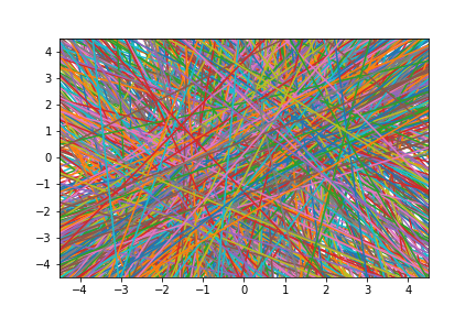
Figure 1: Example line coverage of the estimation grid. Lines are parametrized as $Y_{i}=\mathbf{b}^{\top}\mathbf{X}_{i}$, or by $\beta_{0}=y_{i}-\beta_{1}x_{1_{i}}$.

4.2 Optimization of the Likelihood Functional

The discretized likelihood functional is a $m$-dimensional function, ${\bar{\ell}}^{*}:\mathbbm{R^{m}}\mapsto\mathbbm{R}$. We denote the discretized form of the regularization functionals as, ${\mathcal{R}}^{*}({f^{*}}):\mathbbm{R^{m}}\mapsto\mathbbm{R}$, where $f^{*}=\{f_{j}\}_{j=1}^{m}$

The nonlinear program for the minimization of the conditional average log-likelihood functional was setup as follows:

$$\hat{f_{\bm{\beta}}}=\operatorname*{arg\,min}_{f^{*}}-{\bar{\ell}^{*}}(f^{*}|X,Y)+\alpha\mathcal{R}^{*}(f^{*})$$ (12)

$\begin{array}[]{rcl}\text{subject to}:\sum_{j=1}^{m}f_{j}\Delta b=1,\\ f_{1},f_{2},\ldots,f_{m}\geq 0.\\ \\ \end{array}$

The convexity of the problem allows us to use a trust-region constrained algorithm based on an interior point algorithm for constrained large-scale nonlinear programs developed in Byrd et al., (1999). This particular algorithm excels in solving high-dimensional minimization problems, which is the case for the implementation as $f_{\beta}$ can scale up to the order of thousands in terms of dimensionality. We used the Python implementation of the algorithm in Byrd et al., (1999).

5 Monte Carlo Simulations

We checked the small sample performance of the method in Monte Carlo simulations with two different test examples, one with a normally distributed regressor, and one with a regressor which has bounded support. We compared the results to a kernel-based estimator akin to the one proposed in Hoderlein et al., (2010). We found that the kernel based estimator in our implementation required us to cut-off negative point-estimates and to normalize the final reconstruction, $\hat{f_{\beta}}$, otherwise it produced very poor results.

To test the performance of both methods we conducted a simulation study by generating data for the Random Coefficients model with random slope, and one regressor as specified by equation 11. We then evaluated its ability to reconstruct the underlying distribution of the random coefficients by comparing it to the known true distribution through measuring the empirical mean integrated squared error (MISE) across one-hundred Monte Carlo simulation runs which we repeat for the different sample sizes. We also considered in our study the variance of the integrated squared error (ISE), as we believe stability of the reconstructions is as important to consider as their accuracy.

5.1 Simulation Results for Unbounded Support

We compared the ability of both estimators to reconstruct $f_{\bm{\beta}}$ in the case where the design density has unbounded support. Figure 1 in Section 4 illustrates the case for the full angle coverage.

The data used for these set of simulations was constructed by drawing $X_{1}$ from a normal distribution, $X_{1}\sim\mathcal{N}(0,1)$. The coefficients $\beta_{0}$ and $\beta_{1}$ were sampled from a bimodal, bivariate normal mixture distribution specified as,

$$0.5\mathcal{N}([-1.5,-1.5],\Sigma)+0.5\mathcal{N}([1.5,1.5],\Sigma).$$ (13)

with the simple covariance structure where $\Sigma$ is the identity matrix. Lastly, the variable $Y$ was created using the model equation $y_{i}={\beta_{0}}_{i}+{\beta_{1}}_{i}{x_{1}}_{i}$, hence producing the simulated dataset. Figure 2 shows the shape of the density $f_{\bm{\beta}}$.

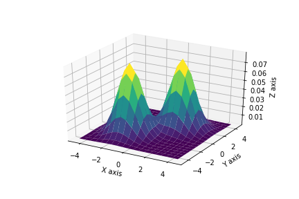
Figure 2: Theoretical $f_{\beta}$.

5.1.1 Simulation Results

The simulation study was done with sample sizes $n=$ {500, 1000, 1500, 3000, 10000}. We used an equidistant grid on the domain $[-4.5,4.5]\times[-4.5,4.5]$ with $m=361$ grid points for $\hat{f_{\bm{\beta}}}$.

As stated in Section 3 we select the parameter $\alpha$ for the RMLE through Lepskii’s principle. However, this parameter choice method did not work well for the bandwidth of the kernel method. So instead we present the results from choosing the reconstruction that has the smallest ISE for each simulation assuming that we have a priori knowledge of the true distribution $f_{\bm{\beta}}$. This means that when comparing the simulation results between the two methods, the kernel-method has a significant advantage over RMLE.

Table 1 contains the statistics 100 Monte Carlo simulation results.

Table 1: Monte Carlo Simulation Results for Unbounded Support

	RMLE		kernel Method
n	MISE	Variance (ISE)	MISE	Variance (ISE)
500	4.043e-05	2.171e-11	9.516e-06	3.361e-12
1,000	2.201e-05	1.566e-10	6.798e-06	1.613e-12
1,500	1.928e-05	1.751e-10	5.720e-06	8.287e-12
3,000	1.399e-05	4.166e-11	4.429e-06	3.675e-13
10,000	9.610e-06	1.926e-12	3.536e-06	8.038e-14

In the case of the RMLE method the MISE, as well as the variance of the ISE, displayed a decreasing trend as sample size increased. The same is true for the kernel method, as a similar decreasing trend is observed for both the MISE and the variance.

Based on the simulation results, the kernel method seems to outperform the RMLE method for the unbounded case with the caveat that these results for the kernel-method were obtained using a superior a priori parameter choice, while the RMLE method used a data-driven parameter choice for $\alpha$.

Figures 4 and 4 are reconstructions using the RMLE method and the kernel method respectively for the unbounded case. The ISE for these reconstructions are 9.136e-06 and 3.149e-06 respectively. It is clear that both methods work well in the case where the support of the distribution of $X_{1}$ is unbounded. The contour plots in Figures 6 and 6 of typical reconstructions suggest the same result.

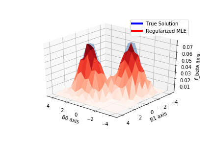
Figure 3: $\hat{f_{\beta}}$ estimate for $n=10,000$ using RMLE

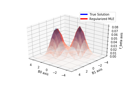
Figure 4: $\hat{f_{\beta}}$ estimate for $n=10,000$ using the kernel method

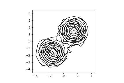
Figure 5: $\hat{f_{\beta}}$ contour using RMLE

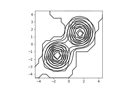
Figure 6: $\hat{f_{\beta}}$ contour using the kernel method

5.2 Simulation Results for Bounded Support

To illustrate the advantage of using RMLE over its kernel-based counterpart we conducted simulations for the case where the design density has bounded support.

To generate the data, the regressor $X_{1}$ was sampled from a uniform distribution on $\small[-0.8,0.8\small]$. The coefficients $\beta_{0}$ and $\beta_{1}$ were sampled from the same bimodal, bivariate normal mixture distribution specified in equation (13). Figure 7 illustrates the limited angle problem caused by the boundedness of $X_{1}$.

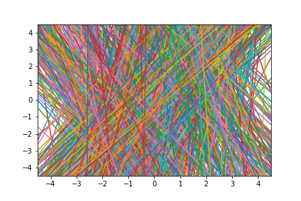
Figure 7: Limited angle coverage of the estimation grid. Lines are parametrized as $Y_{i}={\bm{\beta}}^{\top}\mathbf{X}_{i}$, or by $\beta_{0}=y_{i}-\beta_{1}x_{1_{i}}$.

5.2.1 Simulation Results

The simulation study was done with sample sizes $n=$ {500, 1000, 1500, 3000, 10000} and on the same grid for $\hat{f_{\bm{\beta}}}$ as above. Table 2 contains the statistics for both estimators based on 100 Monte Carlo simulations for each sample sizes.

Table 2: Monte Carlo Simulation Results for Bounded Support

	RMLE		Kernel Method
n	MISE	Variance (ISE)	MISE	Variance (ISE)
500	4.333e-05	1.926e-12	3.320e-05	4.9868e-12
1,000	3.367e-05	8.761e-11	3.173e-05	2.582e-12
1,500	3.007e-05	8.292e-11	3.089e-05	2.121e-12
3,000	2.874e-05	5.730e-11	3.009e-05	1.229e-12
10,000	1.689e-05	2.172e-11	2.922e-05	5.366e-13

The RMLE method shows a decreasing trend in the MISE and the variance of the ISE as the sample size increases. It is noteworthy that the MISEs produced by the RMLE method in the bounded case are not much different to the ones the method produced in the unbounded case.

However, the same cannot be said for the kernel-method. Although it has a smaller variance compared to the RMLE method, the MISEs only decrease marginally as the sample size increases. When compared to the results for the unbounded case, there is a significant difference in the size of the errors produced by the method.

In the case where the design density has bounded support, it is apparent that the Regularized MLE estimator performs considerably better than its kernel-based counterpart in terms of accuracy measured by MISE even with the RMLE method using a data-driven parameter choice, and the kernel-method using an a priori choice for the bandwidth parameter.

Figures 9 and 9 show typical density reconstructions using RMLE and the kernel method with $n=10,000$. The ISEs for the reconstructions were 1.309e-05 and 2.872e-05 respectively. While the kernel method produces a much smoother reconstruction, it suffers from the limited angle problem as seen in the ridging effect that manifests along the pre-dominant directions established by the lines parametrized by the sample. Figures 11 and 11 show the contours of the density reconstructions, $\hat{f}_{\bm{\beta}}$.

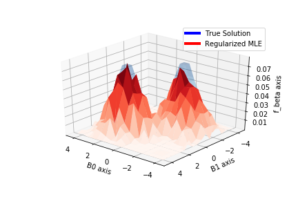
Figure 8: $\hat{f_{\beta}}$ estimate for $n=10,000$ using RMLE

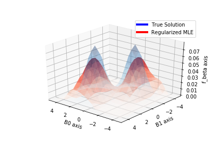
Figure 9: $\hat{f_{\beta}}$ estimate for $n=10,000$ using the kernel method

As stated previously, the parameter $\alpha$ can either be chosen by the statistician or by a data-driven parameter choice rule. If more smoothness in the reconstruction is desired it can be achieved by choosing a larger $\alpha$, or by choosing a regularization term that imposes greater smoothness constraints.

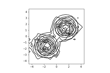
Figure 10: $\hat{f_{\beta}}$ contour using RMLE

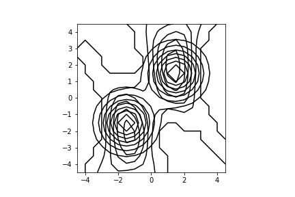
Figure 11: $\hat{f_{\beta}}$ contour using the kernel method

We can conclude that the RMLE method works well in both cases, whereas the kernel method suffers from the problem posed by limited-angle coverage. This robustness with respect to the nature of the data allows us to work with a wider range of data without any complications; furthermore, data with limited support are quite typical in applications for these methods.

6 Application

For a real data application of the estimator we use the data set from Dunker et al., (2019), which are data from the British Family Expenditure Survey from 1997 to 2001 with a sample size of about 33000. The variables we are concerned with being the budget share of food, the log of total expenditure, and the log of food prices. The same transformation on the data done in Dunker et al., (2019) was applied as it leads to more coverage over the estimation grid which improves the estimator’s performance. The model we apply to the data is is motivated by the almost ideal demand system Deaton and Muellbauer, (1980):

$$BS_{i}={\beta_{1}}_{i}\ln(TotalExpenditure_{i})+{\beta_{2}}_{i}\ln(FoodPrices_{i})+\epsilon_{i}$$ (14)

The Ordinary Least-Squares (OLS) results for the model return fixed coefficients as $(\beta_{1},\beta_{2})=(0.085,0.017)$. Figures 13, and 13 show the results using the RMLE method for the same data and model. The results from our estimator suggest that the peak, of $\hat{f}_{\beta_{1},\beta_{2}}$ occurs close to $(0,0)$.

While the OLS results for the fixed coefficients is consistent with what our estimator suggests to be the location of the peak, what it fails to capture is the unobserved heterogeneity present in the population. And, as the result from our estimator shows there is noticeable spread in the estimates for $\beta_{1}$, and $\beta_{2}$ which suggests that a random coefficient model might be a better choice than the fixed coefficient model.

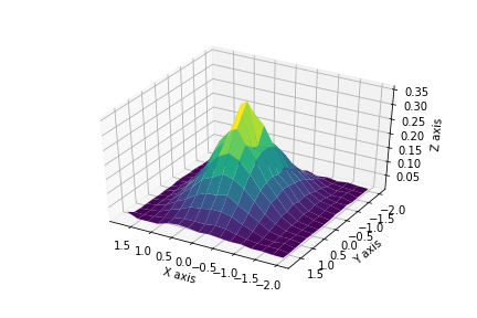
Figure 12: $\hat{f}_{\beta_{1},\beta_{2}}$ estimate.

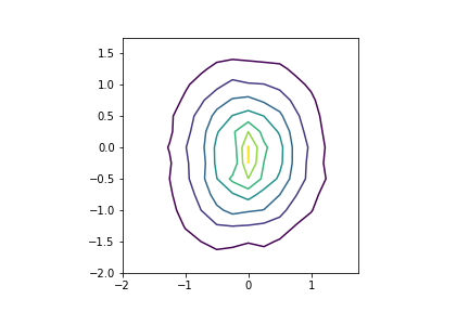
Figure 13: Contour of $\hat{f}_{\beta_{1},\beta_{2}}$

7 Conclusion

We provide an alternative method of estimating the joint distribution of ${\bm{\beta}}$ through Regularized Maximum Likelihood Estimations (RMLE). To combat the instability of the estimate caused by the implicit inversion of the Radon Transform, we apply Tikhonov-type regularization methods.

Compared to its well-known counter part, the kernel method, the RMLE method is more robust with respect to tail behavior of the design density. Although more robust, the method is not completely unaffected by the behavior of the design density, as the rate of decay of the singular values of the operator, and consequently the degree of ill-posedness of the problem, $T$ is determined by the distribution of the regressors.

Monte Carlo simulations illustrate that both methods work well in a scenario where the regressor has unbounded support, but in the case where the regressor has bounded support the RMLE method produces more accurate reconstructions.

Appendix A Proofs

A.1 Proofs of Section 3

Proof of Theorem 1 .

We apply Proposition 4.2 (i) in Hohage and Werner, (2016) for the existence of a minimizer. We have to check the conditions of the theorem. $T$ is a linear integral operator with square integrable which makes it a compact operator. In addition, $-\bar{\ell}(.)$ and $\mathcal{R}:\mathcal{X}\mapsto\mathbbm{R}$ are both convex and lower semi-continuous. Futhermore, $Tf_{\beta}\geq 0\;\text{for all}\;f_{\beta}\in U$. Hence, the conditions of Proposition 4.2 (i) in Hohage and Werner, (2016) are fulfilled.

The uniqueness of the minimizer follows from the strict convexity of $-\bar{\ell}$ which makes the minimization problem (6) strictly convex.

∎

Proof of Theorem 2.

Note that the operator $T$ is equivalent to the $d$-dim Radon transformation if $f_{\bm{\Theta}}$ is bounded away from $0$ on a hemisphere of $\mathbbm{S}^{d-1}$. Hence, $T^{*}T$ has eigen functions $\varphi(x)=\exp(ix\cdot k)$ with $k\in\mathbbm{R}^{d}$. The ill-posedness follows from by Theorem 3.1 in Hertle, (1983). For all $f\in H^{q}(\mathbbm{R}^{d})$, we have $T^{*}Tf\in H^{q+d-1}(\mathbbm{R}^{d})$. Using the spectral calculus yields $(T^{*}T)^{\mu}f\in H^{q+\mu(d-1)}(\mathbbm{R}^{d})$. Hence, for $a<r$, $f_{\beta}$ fulfills the following spectral source condition: There exists $\rho\in H^{a}(\mathbbm{R}^{d})$ such that $(T^{*}T)^{\mu}\rho=f_{\bm{\beta}}$ with $\mu=\frac{r-a}{d-1}$.

As shown in Hofmann and Yamamoto, (2010); Flemming, 2012b ; Flemming, 2012a ; Hohage and Werner, (2016), this spectral source condition implies the variational source condition

$$cD_{\mathcal{R}}^{f_{\beta}^{*}}(f,f_{\bm{\beta}})\leq\mathcal{R}(f)-\mathcal{R}(f_{\bm{\beta}})+\lambda(\|f_{S|{\bm{\Theta}}}-Tf\|^{2}_{L^{2}})$$

with some $c>0$, $\mathcal{R}=\|\cdot\|_{H^{a}}^{2}$, and $\lambda(x)=x^{\frac{2\mu}{2\mu+1}}=x^{\frac{2(r-a)}{2(r-a)+d-1}}$ if $\mu\leq 1$.

We apply the inequality $\|\varphi-\psi\|_{L^{2}}^{2}\leq\left(\frac{2}{3}\|\varphi\|_{\infty}+\frac{4}{3}\|\psi\|_{\infty}\right)\mathbbm{KL}(\varphi;\psi)$ which holds for all nonnegative functions $\varphi,\psi\in L^{\infty}(\mathbbm{R}^{d})$ with $\varphi-\psi\in L^{2}(\mathbbm{R}^{d})$, see Borwein and Lewis, (1991); Dunker and Hohage, (2014). Since $\lambda$ is a power function, we get

$$\lambda(\|f_{S|{\bm{\Theta}}}-Tf\|^{2}_{L^{2}}) \leq\lambda\left(\left(\frac{2}{3}\|f_{S|{\bm{\Theta}}}\|_{\infty}+\frac{4}{3}\|Tf\|_{\infty}\right)\mathbbm{KL}(f_{S|{\bm{\Theta}}};Tf)\right)$$

$$=\lambda\left(\frac{2}{3}\|f_{S|{\bm{\Theta}}}\|_{\infty}+\frac{4}{3}\|Tf\|_{\infty}\right)\lambda\left(\mathbbm{KL}(f_{S|{\bm{\Theta}}};Tf)\right)$$

Hence, there is a constant $c^{\prime}>0$ such that

$$c^{\prime}D_{\mathcal{R}}^{f_{\beta}^{*}}(f,f_{\bm{\beta}})\leq\mathcal{R}(f)-\mathcal{R}(f_{\bm{\beta}})+\lambda\left(\mathbbm{KL}(f_{S|{\bm{\Theta}}};Tf)\right)$$

This proves the theorem.

∎

Proof of Theorem 3.

This is a standard result in variational regularization theory. See for example Theorem 4.3 in Werner and Hohage, (2012).

∎

Proof of Theorem 4.

We apply Theorem 3 to the special case of Theorem 2. In this case $\lambda(x)=x^{\frac{2(r-a)}{2(r-a)+d-1}}$ is differentiable. Hence, $-\partial(-\lambda)(x)=\lambda^{\prime}(x)=\frac{2(r-a)}{2(r-a)+d-1}x^{\frac{1-d}{2(r-a)+d-1}}$. Replacing $x$ by $n^{-1/2}$ gives the parameter choice. The convergence rate is given by $\lambda(n^{-1/2})=n^{-\frac{r-a}{2(r-a)+d-1}}$.

∎

Proof of Theorem 5.

The first part of the theorem is a consequence of Theorem 5.1 in Werner and Hohage, (2012). The second part of the theorem is using the convergence rate from Theorem 4 together with the first part of the theorem.

$$\lambda\left(\frac{\ln(n)}{\sqrt{n}}\right)=\left(\frac{\ln(n)}{\sqrt{n}}\right)^{\frac{2(r-a)}{2(r-a)+d-1}}=\ln(x)^{\frac{2(r-a)}{2(r-a)+d-1}}~{}n^{-\frac{r-a}{2(r-a)+d-1}}~{}.$$

∎

References

- Bauer and Hohage, (2005) Bauer, F. and Hohage, T. (2005). A lepskij-type stopping rule for regularized newton methods. Inverse Problems, 21(6):1975–1991.
- Benning and Burger, (2018) Benning, M. and Burger, M. (2018). Modern regularization methods for inverse problems. Acta Numerica, 27:1–111.
- Beran et al., (1996) Beran, R., Feuerverger, A., and Hall, P. (1996). On nonparametric estimation of intercept and slope distributions in random coefficient regression. Ann. Statist., 24(6):2569–2592.
- Beran and Hall, (1992) Beran, R. and Hall, P. (1992). Estimating coefficient distributions in random coefficient regressions. Ann. Statist., 20(4):1970–1984.
- Berry et al., (1995) Berry, S., Levinsohn, J., and Pakes, A. (1995). Automobile prices in market equilibrium. Econometrica, 63(4):841–890.
- Berry and Pakes, (2007) Berry, S. and Pakes, A. (2007). The pure characteristics demand model. Internat. Econom. Rev., 48(4):1193–1225.
- Borwein and Lewis, (1991) Borwein, J. M. and Lewis, A. S. (1991). Convergence of best entropy estimates. SIAM J. Optim., 1(2):191–205.
- Breunig and Hoderlein, (2018) Breunig, C. and Hoderlein, S. (2018). Specification testing in random coefficient models. Quantitative Economics, 9(3):1371–1417.
- Butucea et al., (2007) Butucea, C., Guţă, M., and Artiles, L. (2007). Minimax and adaptive estimation of the Wigner function in quantum homodyne tomography with noisy data. Ann. Statist., 35(2):465–494.
- Byrd et al., (1999) Byrd, R. H., Hribar, M. E., and Nocedal, J. (1999). An interior point algorithm for large-scale nonlinear programming. SIAM Journal on Optimization, 9(4):877–900.
- Deaton and Muellbauer, (1980) Deaton, A. and Muellbauer, J. (1980). An almost ideal demand system. American Economic Review, 70:312–326.
- Dubé et al., (2012) Dubé, J.-P., Fox, J. T., and Su, C.-L. (2012). Improving the numerical performance of static and dynamic aggregate discrete choice random coefficients demand estimation. Econometrica, 80(5):2231–2267.
- Dunker et al., (2019) Dunker, F., Eckle, K., Proksch, K., and Schmidt-Hieber, J. (2019). Tests for qualitative features in the random coefficients model. Electron. J. Statist., 13(2):2257–2306.
- Dunker et al., (2013) Dunker, F., Hoderlein, S., and Kaido, H. (2013). Random coefficients in static games of complete information. cemmap Working Papers, CWP12/13.
- Dunker et al., (2017) Dunker, F., Hoderlein, S., and Kaido, H. (2017). Nonparametric identification of random coefficients in endogenous and heterogeneous aggregate demand models. cemmap Working Papers, CWP11/17.
- Dunker et al., (2018) Dunker, F., Hoderlein, S., Kaido, H., and Sherman, R. (2018). Nonparametric identification of the distribution of random coefficients in binary response static games of complete information. Journal of Econometrics, 206(1):83 – 102.
- Dunker and Hohage, (2014) Dunker, F. and Hohage, T. (2014). On parameter identification in stochastic differential equations by penalized maximum likelihood. Inverse Problems, 30(9):095001.
- Feuerverger and Vardi, (2000) Feuerverger, A. and Vardi, Y. (2000). Positron emission tomography and random coefficients regression. Ann. Inst. Statist. Math., 52(1):123–138.
- Flemming, (2010) Flemming, J. (2010). Theory and examples of variational regularization with non-metric fitting functionals. J. Inverse Ill-Posed Probl., 18(6):677–699.
- (20) Flemming, J. (2012a). Generalized Tikhonov regularization and modern convergence rate theory in Banach spaces. Shaker Verlag, Aachen.
- (21) Flemming, J. (2012b). Solution smoothness of ill-posed equations in hilbert spaces: four concepts and their cross connections. Applicable Analysis, 91(5):1029–1044.
- Flemming and Hofmann, (2010) Flemming, J. and Hofmann, B. (2010). A new approach to source conditions in regularization with general residual term. Numerical functional analysis and optimization, 31(3):254–284.
- Fox and Gandhi, (2016) Fox, J. T. and Gandhi, A. (2016). Nonparametric identification and estimation of random coefficients in multinomial choice models. The RAND Journal of Economics, 47(1):118–139.
- Gautier and Hoderlein, (2012) Gautier, E. and Hoderlein, S. (2012). A triangular treatment effect model with random coefficients in the selection equation. cemmap Working Papers, CWP39/12.
- Gautier and Kitamura, (2013) Gautier, E. and Kitamura, Y. (2013). Nonparametric estimation in random coefficients binary choice models. Econometrica, 81(2):581–607.
- Greenland, (2000) Greenland, S. (2000). When should epidemiologic regressions use random coefficients? Biometrics, 56(3):915–921.
- Gustafson and Greenland, (2006) Gustafson, P. and Greenland, S. (2006). The performance of random coefficient regression in accounting for residual confounding. Biometrics, 62(3):760–768.
- Heiss et al., (2019) Heiss, F., Hetzenecker, S., and Osterhaus, M. (2019). Nonparametric estimation of the random coefficients model: An elastic net approach. arXiv preprint arXiv:1909.08434.
- Hertle, (1983) Hertle, A. (1983). Continuity of the radon transform and its inverse on euclidean space. Mathematische Zeitschrift, 184(2):165–192.
- Hoderlein et al., (2017) Hoderlein, S., Holzmann, H., and Meister, A. (2017). The triangular model with random coefficients. Journal of Econometrics, 201(1):144 – 169.
- Hoderlein et al., (2010) Hoderlein, S., Klemelä, J., and Mammen, E. (2010). Analyzing the random coefficient model nonparametrically. Econometric Theory, 26(3):804–837.
- Hofmann and Yamamoto, (2010) Hofmann, B. and Yamamoto, M. (2010). On the interplay of source conditions and variational inequalities for nonlinear ill-posed problems. Applicable Analysis, 89(11):1705–1727.
- Hohage and Miller, (2019) Hohage, T. and Miller, P. (2019). Optimal convergence rates for sparsity promoting wavelet-regularization in besov spaces. Inverse Problems, 35(6):065005.
- Hohage and Weidling, (2017) Hohage, T. and Weidling, F. (2017). Characterizations of variational source conditions, converse results, and maxisets of spectral regularization methods. SIAM Journal on Numerical Analysis, 55(2):598–620.
- Hohage and Werner, (2013) Hohage, T. and Werner, F. (2013). Iteratively regularized Newton-type methods for general data misfit functionals and applications to Poisson data. Numer. Math., 123(4):745–779.
- Hohage and Werner, (2016) Hohage, T. and Werner, F. (2016). Inverse problems with poisson data: statistical regularization theory, applications and algorithms. Inverse Problems, 32(9):093001.
- Hohmann and Holzmann, (2016) Hohmann, D. and Holzmann, H. (2016). Weighted angle radon transform: Convergence rates and efficient estimation. Statistica Sinica., 26(1):157–175.
- Holzmann and Meister, (2020) Holzmann, H. and Meister, A. (2020). Rate-optimal nonparametric estimation for random coefficient regression models. Bernoulli, fourthcomming.
- Hsiao, (2014) Hsiao, C. (2014). Analysis of Panel Data. Cambridge University Press. Cambridge Books Online.
- Hsiao and Pesaran, (2004) Hsiao, C. and Pesaran, M. H. (2004). Random Coefficient Panel Data Models. CESifo Working Paper Series 1233, CESifo Group Munich.
- Ichimura and Thompson, (1998) Ichimura, H. and Thompson, T. (1998). Maximum likelihood estimation of a binary choice model with random coefficients of unknown distribution. Journal of Econometrics, 86(2):269 – 295.
- Lepskiĭ, (1991) Lepskiĭ, O. V. (1991). Asymptotically minimax adaptive estimation. I. Upper bounds. Optimally adaptive estimates. Teor. Veroyatnost. i Primenen., 36(4):645–659.
- Lepskiĭ, (1992) Lepskiĭ, O. V. (1992). On problems of adaptive estimation in white Gaussian noise. In Topics in nonparametric estimation, volume 12 of Adv. Soviet Math., pages 87–106. Amer. Math. Soc., Providence, RI.
- Masten, (2018) Masten, M. A. (2018). Random coefficients on endogenous variables in simultaneous equations models. The Review of Economic Studies, 85(2):1193–1250.
- Masten and Torgovitsky, (2016) Masten, M. A. and Torgovitsky, A. (2016). Identification of instrumental variable correlated random coefficients models. The Review of Economics and Statistics, 98(5):1001–1005.
- Mathé, (2006) Mathé, P. (2006). The lepskii principle revisited. Inverse Problems, 22(3):L11–L15.
- Nevo, (2001) Nevo, A. (2001). Measuring market power in the ready-to-eat cereal industry. Econometrica, 69(2):307–342.
- Petrin, (2002) Petrin, A. (2002). Quantifying the benefits of new products: The case of the minivan. Journal of Political Economy, 110(4):705–729.
- Scherzer et al., (2009) Scherzer, O., Grasmair, M., Grossauer, H., Haltmeier, M., and Lenzen, F. (2009). Variational methods in imaging, volume 167 of Applied Mathematical Sciences. Springer, New York.
- Schuster et al., (2012) Schuster, T., Kaltenbacher, B., Hofmann, B., and Kazimierski, K. S. (2012). Regularization methods in Banach spaces, volume 10 of Radon Series on Computational and Applied Mathematics. Walter de Gruyter GmbH & Co. KG, Berlin.
- Tsybakov, (2000) Tsybakov, A. (2000). On the best rate of adaptive estimation in some inverse problems. Comptes Rendus de l’Académie des Sciences. Série I. Mathématique, 330(9):835–840.
- Weidling et al., (2020) Weidling, F., Sprung, B., and Hohage, T. (2020). Optimal convergence rates for tikhonov regularization in besov spaces. SIAM Journal on Numerical Analysis, 58(1):21–47.
- Werner, (2018) Werner, F. (2018). Adaptivity and oracle inequalities in linear statistical inverse problems: a (numerical) survey. In Hofmann, B., Leitao, A., and Zubelli, J. P., editors, New Trends in Parameter Identification for Mathematical Models. Birkhäuser, Basel.
- Werner and Hohage, (2012) Werner, F. and Hohage, T. (2012). Convergence rates in expectation for Tikhonov-type regularization of inverse problems with Poisson data. Inverse Problems, 28(10):104004, 15.