On the Importance of Effectively Adapting Pretrained Language Models for Active Learning

Abstract

Recent Active Learning (AL) approaches in Natural Language Processing (NLP) proposed using off-the-shelf pretrained language models (LMs). In this paper, we argue that these LMs are not adapted effectively to the downstream task during AL and we explore ways to address this issue. We suggest to first adapt the pretrained LM to the target task by continuing training with all the available unlabeled data and then use it for AL. We also propose a simple yet effective fine-tuning method to ensure that the adapted LM is properly trained in both low and high resource scenarios during AL. Our experiments demonstrate that our approach provides substantial data efficiency improvements compared to the standard fine-tuning approach, suggesting that a poor training strategy can be catastrophic for AL.

1 Introduction

Active Learning (AL) is a method for training supervised models in a data-efficient way Cohn et al. (1996); Settles (2009). It is especially useful in scenarios where a large pool of unlabeled data is available but only a limited annotation budget can be afforded; or where expert annotation is prohibitively expensive and time consuming. AL methods iteratively alternate between (i) model training with the labeled data available; and (ii) data selection for annotation using a stopping criterion, e.g. until exhausting a fixed annotation budget or reaching a pre-defined performance on a held-out dataset.

Data selection is performed by an acquisition function that ranks unlabeled data points by some informativeness metric aiming to improve over random selection, using either uncertainty Lewis and Gale (1994); Cohn et al. (1996); Gal et al. (2017); Kirsch et al. (2019); Zhang and Plank (2021), diversity Brinker (2003); Bodó et al. (2011); Sener and Savarese (2018), or both Ducoffe and Precioso (2018); Ash et al. (2020); Yuan et al. (2020); Margatina et al. (2021).

Previous AL approaches in NLP use task-specific neural models that are trained from scratch at each iteration Shen et al. (2017); Siddhant and Lipton (2018); Prabhu et al. (2019); Ikhwantri et al. (2018); Kasai et al. (2019). However, these models are usually outperformed by pretrained language models (LMs) adapted to end-tasks Howard and Ruder (2018), making them suboptimal for AL. Only recently, pretrained LMs such as Bert Devlin et al. (2019) have been introduced in AL settings Yuan et al. (2020); Ein-Dor et al. (2020); Shelmanov et al. (2021); Karamcheti et al. (2021); Margatina et al. (2021). Still, they are trained at each AL iteration with a standard fine-tuning approach that mainly includes a pre-defined number of training epochs, which has been demonstrated to be unstable, especially in small datasets Zhang et al. (2020); Dodge et al. (2020); Mosbach et al. (2021). Since AL includes both low and high data resource settings, the AL model training scheme should be robust in both scenarios.

To address these limitations, we introduce a suite of effective training strategies for AL (§2). Contrary to previous work Yuan et al. (2020); Ein-Dor et al. (2020); Margatina et al. (2021) that also use Bert Devlin et al. (2019), our proposed method accounts for various data availability settings and the instability of fine-tuning. First, we continue pretraining the LM with the available unlabeled data to adapt it to the task-specific domain. This way, we leverage not only the available labeled data at each AL iteration, but the entire unlabeled pool. Second, we further propose a simple yet effective fine-tuning method that is robust in both low and high resource data settings for AL.

We explore the effectiveness of our approach on five standard natural language understandings tasks with various acquisition functions, showing that it outperforms all baselines (§3). We also conduct an analysis to demonstrate the importance of effective adaptation of pretrained models for AL (§4). Our findings highlight that the LM adaptation strategy can be more critical than the actual data acquisition strategy.

2 Adapting & Fine-tuning Pretrained Models for Active Learning

Given a downstream classification task with $C$ classes, a typical AL setup consists of a pool of unlabeled data $\mathcal{D}_{\textbf{pool}}$, a model $\mathcal{M}$, an annotation budget $b$ of data points and an acquisition function $a(.)$ for selecting $k$ unlabeled data points for annotation (i.e. acquisition size) until $b$ runs out. The AL performance is assessed by training a model on the actively acquired dataset and evaluating on a held-out test set $\mathcal{D}_{\textbf{test}}$.

Adaptation (tapt)

Inspired by recent work on transfer learning that shows improvements in downstream classification performance by continuing the pretraining of the LM with the task data Howard and Ruder (2018) we add an extra step to the AL process by continuing pretraining the LM (i.e. Task-Adaptive Pretraining tapt), as in Gururangan et al. (2020). Formally, we use an LM, such as Bert Devlin et al. (2019), $\mathcal{P}(x;W_{0})$ with weights $W_{0}$, that has been already pretrained on a large corpus. We fine-tune $\mathcal{P}(x;W_{0})$ with the available unlabeled data of the downstream task $\mathcal{D}_{\textbf{pool}}$, resulting in the task-adapted LM $\mathcal{P}_{\text{TAPT}}(x;W_{0}^{\prime})$ with new weights $W_{0}^{\prime}$ (cf. line 2 of algorithm 1).

Fine-tuning (ft+)

We now use the adapted LM $\mathcal{P}_{\text{TAPT}}(x;W_{0}^{\prime})$ for AL. At each iteration $i$, we initialize our model $\mathcal{M}_{i}$ with the pretrained weights $W_{0}^{\prime}$ and we add a task-specific feedforward layer for classification with weights $W_{c}$ on top of the [CLS] token representation of Bert-based $\mathcal{P}_{\text{TAPT}}$. We fine-tune the classification model $\mathcal{M}_{i}(x;[W_{0}^{\prime},W_{c}])$ with all $x\in\mathcal{D}_{\textbf{lab}}$. (cf. line 6 to 8 of algorithm 1).

Recent work in AL Ein-Dor et al. (2020); Yuan et al. (2020) uses the standard fine-tuning method proposed in Devlin et al. (2019) which includes a fixed number of $3$ training epochs, learning rate warmup over the first $10\%$ of the steps and AdamW optimizer Loshchilov and Hutter (2019) without bias correction, among other hyperparameters.

We follow a different approach by taking into account insights from few-shot fine-tuning literature Mosbach et al. (2021); Zhang et al. (2020); Dodge et al. (2020) that proposes longer fine-tuning and more evaluation steps during training.  We combine these guidelines to our fine-tuning approach by using early stopping with $20$ epochs based on the validation loss, learning rate $2e-5$, bias correction and $5$ evaluation steps per epoch. However, increasing the number of epochs from $3$ to $20$, also increases the warmup steps ($10\%$ of total steps) almost $7$ times. This may be problematic in scenarios where the dataset is large but the optimal number of epochs may be small (e.g. $2$ or $3$). To account for this limitation in our AL setting where the size of training set changes at each iteration, we propose to select the warmup steps as $min(10\%\text{ of total steps},100)$. We denote standard fine-tuning as sft and our approach as ft+.

1

2

3

Input: unlabeled data $\mathcal{D}_{\textbf{pool}}$, pretrained LM $\mathcal{P}(x;W_{0})$, acquisition size $k$, AL iterations $T$, acquisition function $a$

4

5$\mathcal{D}_{\textbf{lab}}\leftarrow\emptyset$

6

7$\mathcal{P}_{\text{TAPT}}(x;W_{0}^{\prime})\leftarrow$ Train $\mathcal{P}(x;W_{0})$ on $\mathcal{D}_{\textbf{pool}}$

8

9$\mathcal{Q}_{0}\leftarrow$ RANDOM$(.),|\mathcal{Q}_{0}|=k$

10

11$\mathcal{D}_{\textbf{lab}}=\mathcal{D}_{\textbf{lab}}\cup\mathcal{Q}_{0}$

12 $\mathcal{D}_{\textbf{pool}}=\mathcal{D}_{\textbf{pool}}\setminus\mathcal{Q}_{0}$

13 for  $i\leftarrow 1$ to $T$ do

14       $\mathcal{M}_{i}(x;[W_{0}^{\prime},W_{c}])\leftarrow$ Initialize from $\mathcal{P}_{\text{TAPT}}(x;W_{0}^{\prime})$

15       $\mathcal{M}_{i}(x;W_{i})\leftarrow$ Train model on $\mathcal{D}_{\textbf{lab}}$

16       $\mathcal{Q}_{i}\leftarrow a(\mathcal{M}_{i},\mathcal{D}_{\textbf{pool}},k)$

17       $\mathcal{D}_{\textbf{lab}}=\mathcal{D}_{\textbf{lab}}\cup\mathcal{Q}_{i}$

18       $\mathcal{D}_{\textbf{pool}}=\mathcal{D}_{\textbf{pool}}\setminus\mathcal{Q}_{i}$

19      

20 end for

Output: $\mathcal{D}_{\textbf{lab}}$

Algorithm 1 AL with Pretrained LMs

datasets	train	val	test	$k$	$C$
trec-6	$4.9$K	$546$	$500$	$1\%$	$6$
dbpedia	$20$K	$2$K	$70$K	$1$%	$14$
imdb	$22.5$K	$2.5$K	$25$K	$1$%	$2$
sst-2	$60.6$K	$6.7$K	$871$	$1$%	$2$
agnews	$114$K	$6$K	$7.6$K	$0.5\%$	$4$

Table 1: Datasets statistics for $\mathcal{D}_{\textbf{pool}}$, $\mathcal{D}_{\textbf{val}}$ and $\mathcal{D}_{\textbf{test}}$ respectively. $k$ stands for the acquisition size (% of $\mathcal{D}_{\textbf{pool}}$) and $C$ the number of classes.

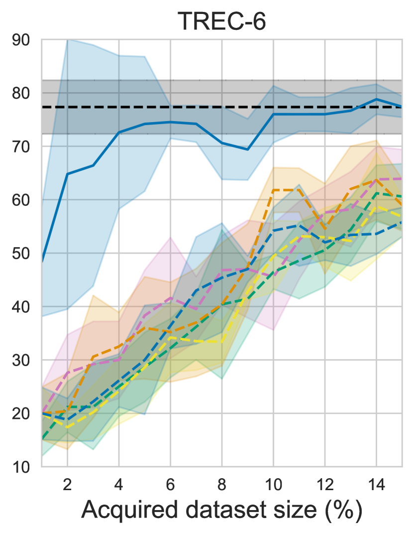
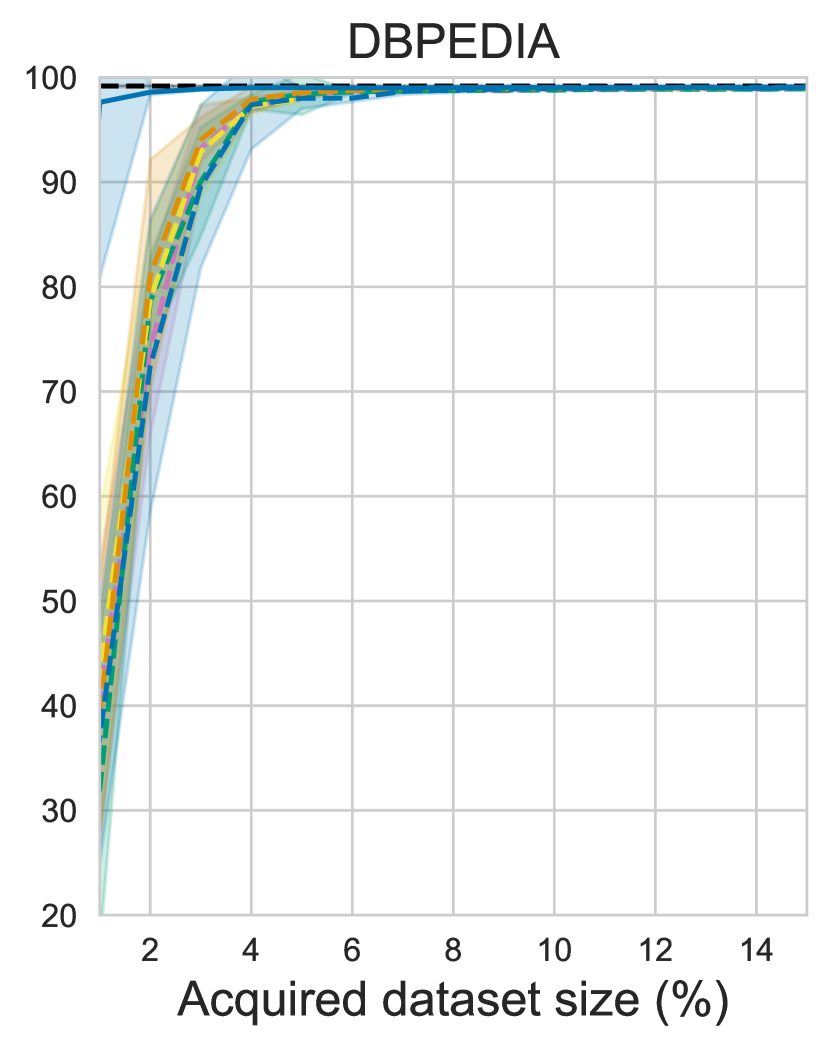
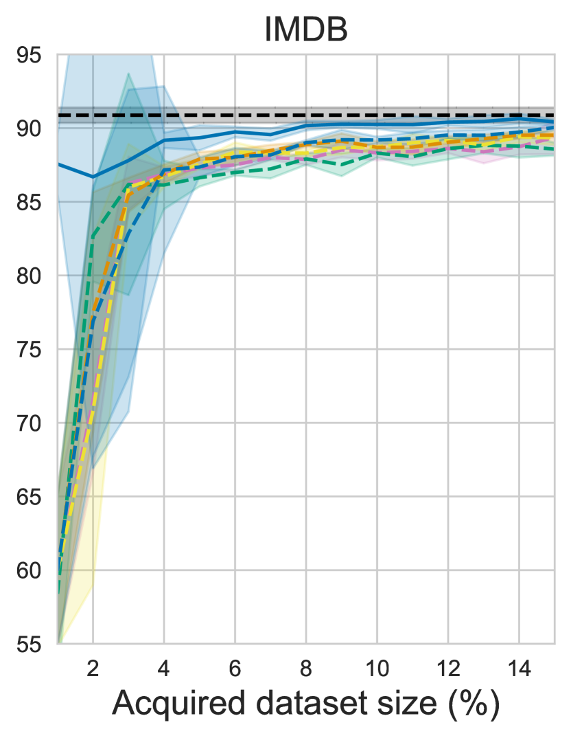
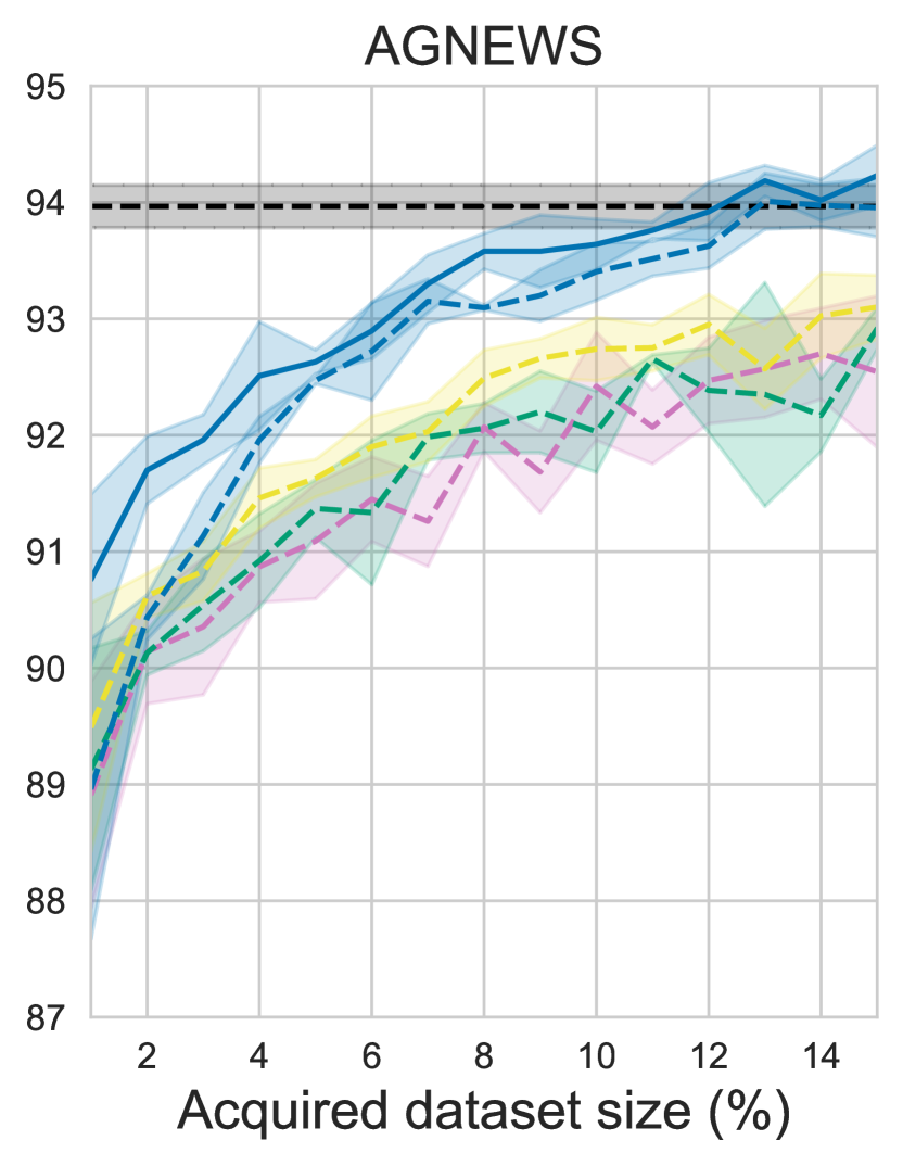
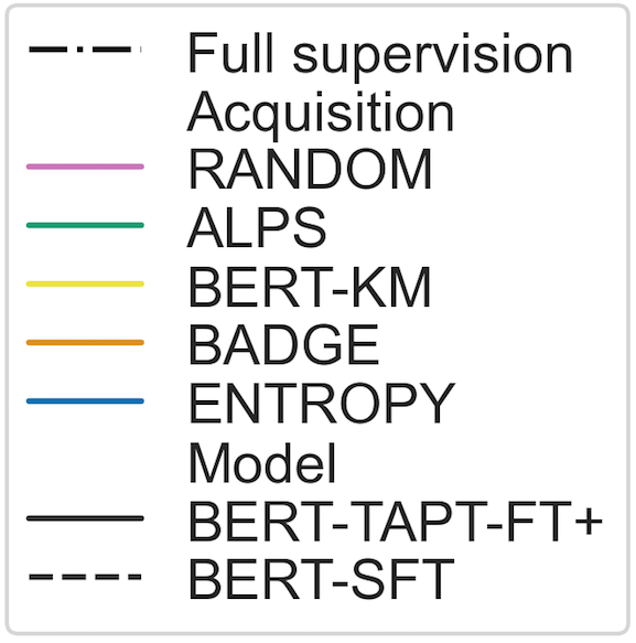
Figure 1: Test accuracy during AL iterations. We plot the median and standard deviation across five runs.

3 Experiments & Results

Data

We experiment with five diverse natural language understanding tasks: question classification (trec-6; Voorhees and Tice (2000)), sentiment analysis (imdb; Maas et al. (2011), sst-2 Socher et al. (2013)) and topic classification (dbpedia, agnews; Zhang et al. (2015)), including binary and multi-class labels and varying dataset sizes (Table 1). More details can be found in Appendix A.1.

Experimental Setup

We perform all AL experiments using BERT-base Devlin et al. (2019) and Entropy, BertKM, Alps Yuan et al. (2020), Badge Ash et al. (2020) and Random (baseline) as the acquisition functions. We pair our proposed training approach tapt-ft+ with Entropy acquisition. We refer the reader to Appendix A for an extended description of our experimental setup, including the datasets used (§A.1), the training and AL details (§A.2), the model hyperparameters (§A.3) and the baselines (§A.4).

Results

Figure 1 shows the test accuracy during AL iterations. We first observe that our proposed approach (tapt-ft+) achieves large data efficiency reaching the full-dataset performance within the $15\%$ budget for all datasets, in contrast to the standard AL approach (Bert-sft). The effectiveness of our approach is mostly notable in the smaller datasets. In trec-6, it achieves the goal accuracy with almost $10\%$ annotated data, while in dbpedia only in the first iteration with $2\%$ of the data. After the first AL iteration in imdb, tapt-ft+, it achieves only $2.5$ points of accuracy lower than the performance when using $100\%$ of the data. In the larger sst-2 and agnews datasets, it is closer to the baselines but still outperforms them, achieving the full-dataset performance with $8\%$ and $12\%$ of the data respectively. We also observe that in all five datasets, the addition of our proposed pretraining step (tapt) and fine-tuning technique (ft+) leads to large performance gains, especially in the first AL iterations. This is particularly evident in trec-6, dbpedia and imdb datasets, where after the first AL iteration (i.e. equivalent to $2\%$ of training data) tapt+ft+ with Entropy is $45$, $30$ and $12$ points in accuracy higher than the Entropy baseline with Bert and sft.

Training vs. Acquisition Strategy

We finally observe that the performance curves of the various acquisition functions considered (i.e. dotted lines) are generally close to each other, suggesting that the choice of the acquisition strategy may not affect substantially the AL performance in certain cases. In other words, we conclude that the training strategy can be more important than the acquisition strategy. We find that uncertainty sampling with Entropy is generally the best performing acquisition function, followed by Badge. Still, finding a universally well-performing acquisition function, independent of the training strategy, is an open research question.

4 Analysis & Discussion

4.1 Task-Adaptive Pretraining

We first present details of our implementation of tapt (§2) and reflect on its effectiveness in the AL pipeline. Following Gururangan et al. (2020), we continue pretraining Bert for the MLM task using all the unlabeled data $\mathcal{D}_{\textbf{pool}}$ for all datasets separately. We plot the learning curves of Bert-tapt for all datasets in Figure 2. We first observe that the masked LM loss is steadily decreasing for dbpedia, imdb and agnews across optimization steps, which correlates with the high early AL performance gains of tapt in these datasets (Fig. 1). We also observe that the LM overfits in trec-6 and sst-2 datasets. We attribute this to the very small training dataset of trec-6 and the informal textual style of sst-2. Despite the fact that the sst-2 dataset includes approximately $67$K of training data, the sentences are very short (i.e. average length of $9.4$ words per sentence). We hypothesize the LM overfits because of the lack of long and more diverse sentences. We provide more details on tapt at the Appendix B.1.

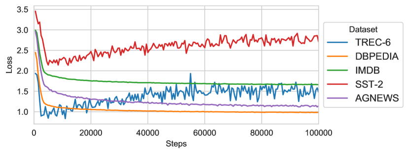
Figure 2: Validation MLM loss during tapt.

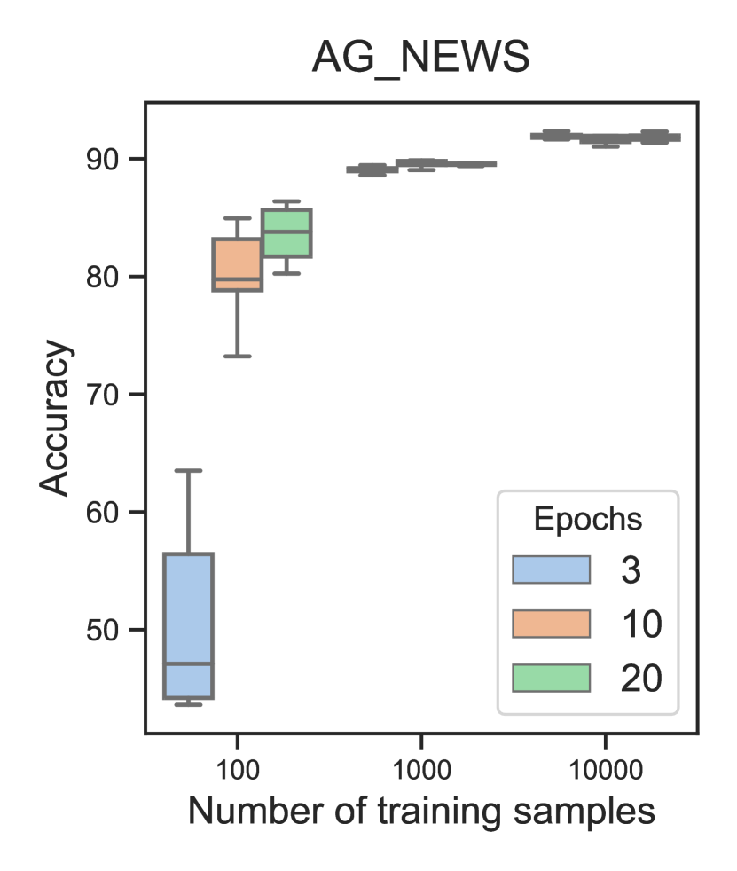
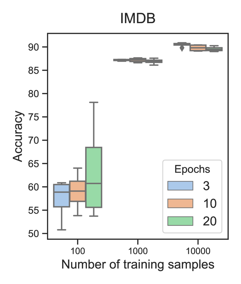
Figure 3: Few-shot standard Bert fine-tuning.

4.2 Few-shot Fine-tuning

In this set of experiments, we aim to highlight that it is crucial to consider the few-shot learning problem in the early AL stages, which is often neglected in literature. This is more important when using pretrained LMs, since they are overparameterized models that require adapting their training scheme in low data settings to ensure robustness.

To illustrate the potential ineffectiveness of standard fine-tuning (sft), we randomly undersample the agnews and imdb datasets to form low, medium and high resource data settings (i.e. $100$, $1,000$ and $10,000$ training samples), and train Bert for a fixed number of $3$, $10$, and $20$ epochs. We repeat this process with $10$ different random seeds to account for stochasticity in sampling and we plot the test accuracy in Figure 3. Figure 3 shows that sft is suboptimal for low data settings (e.g. $100$ samples), indicating that more optimization steps (i.e. epochs) are needed for the model to adapt to the few training samples Zhang et al. (2020); Mosbach et al. (2021). As the training samples increase (e.g. $1,000$), fewer epochs are often better. It is thus evident that there is not a clearly optimal way to choose a predefined number of epochs to train the model given the number of training examples. This motivates the need to find a fine-tuning policy for AL that effectively adapts to the data resource setting of each iteration (independently of the number of training examples or dataset), which is mainly tackled by our proposed fine-tuning approach ft+ (§2).

4.3 Ablation Study

We finally conduct an ablation study to evaluate the contribution of our two proposed steps to the AL pipeline; the pretraining step (tapt) and fine-tuning method (ft+). We show that the addition of both methods provides large gains compared to standard fine-tuning (sft) in terms of accuracy, data efficiency and uncertainty calibration. We compare Bert with sft, Bert with ft+ and Bert-tapt with ft+. Along with test accuracy, we also evaluate each model using uncertainty estimation metrics Ovadia et al. (2019): Brier score, negative log likelihood (NLL), expected calibration error (ECE) and entropy. A well-calibrated model should have high accuracy and low uncertainty.

Figure 4 shows the results for the smallest and largest datasets, trec-6 and agnews respectively. For trec-6, training Bert with our fine-tuning approach ft+ provides large gains both in accuracy and uncertainty calibration, showing the importance of fine-tuning the LM for a larger number of epochs in low resource settings. For the larger dataset, agnews, we see that Bert with sft performs equally to ft+ which is the ideal scenario. We see that our fine-tuning approach does not deteriorate the performance of Bert given the large increase in warmup steps, showing that our simple strategy provides robust results in both high and low resource settings. After demonstrating that ft+ yields better results than sft, we next compare Bert-tapt-ft+ against Bert-ft+. We observe that in both datasets Bert-tapt outperforms Bert, with this being particularly evident in the early iterations. This confirms our hypothesis that by implicitly using the entire pool of unlabeled data for extra pretraining (tapt), we boost the performance of the AL model using less data.

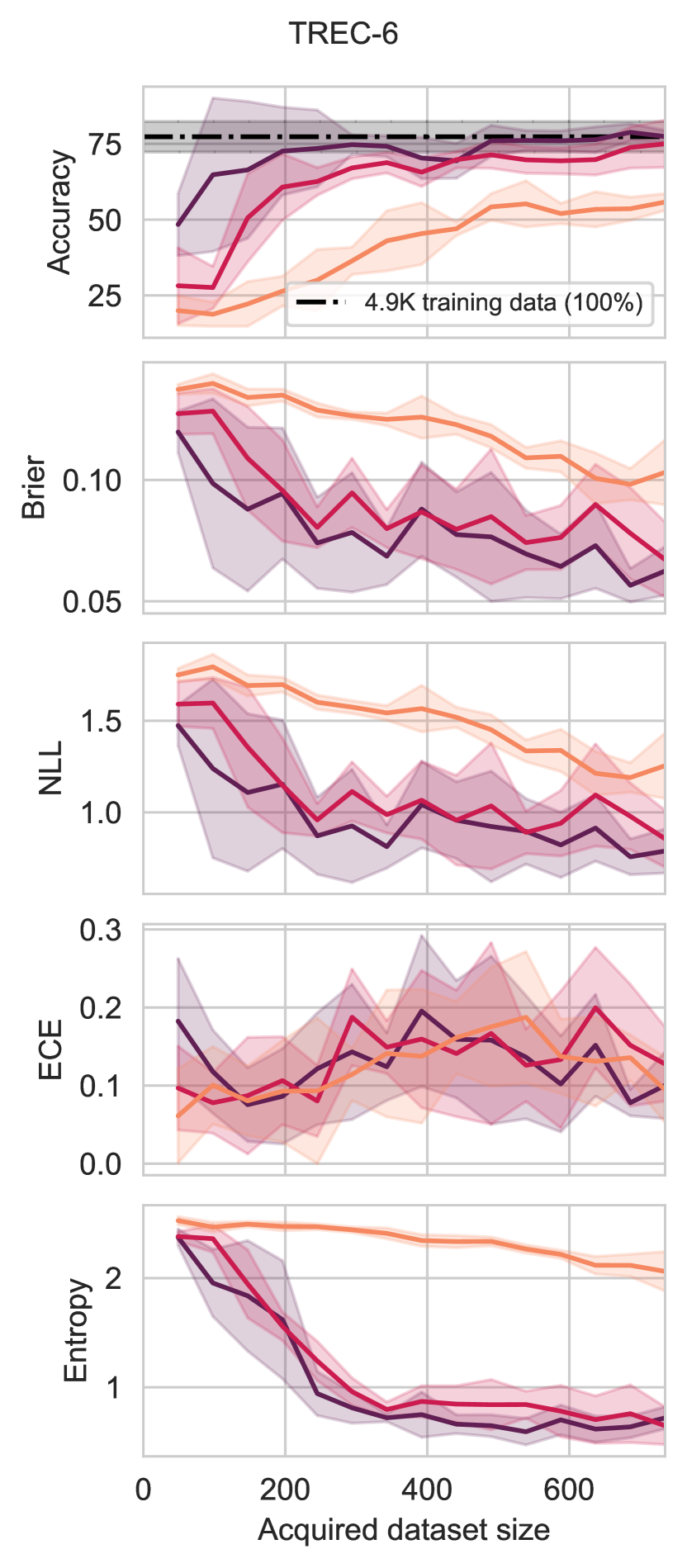
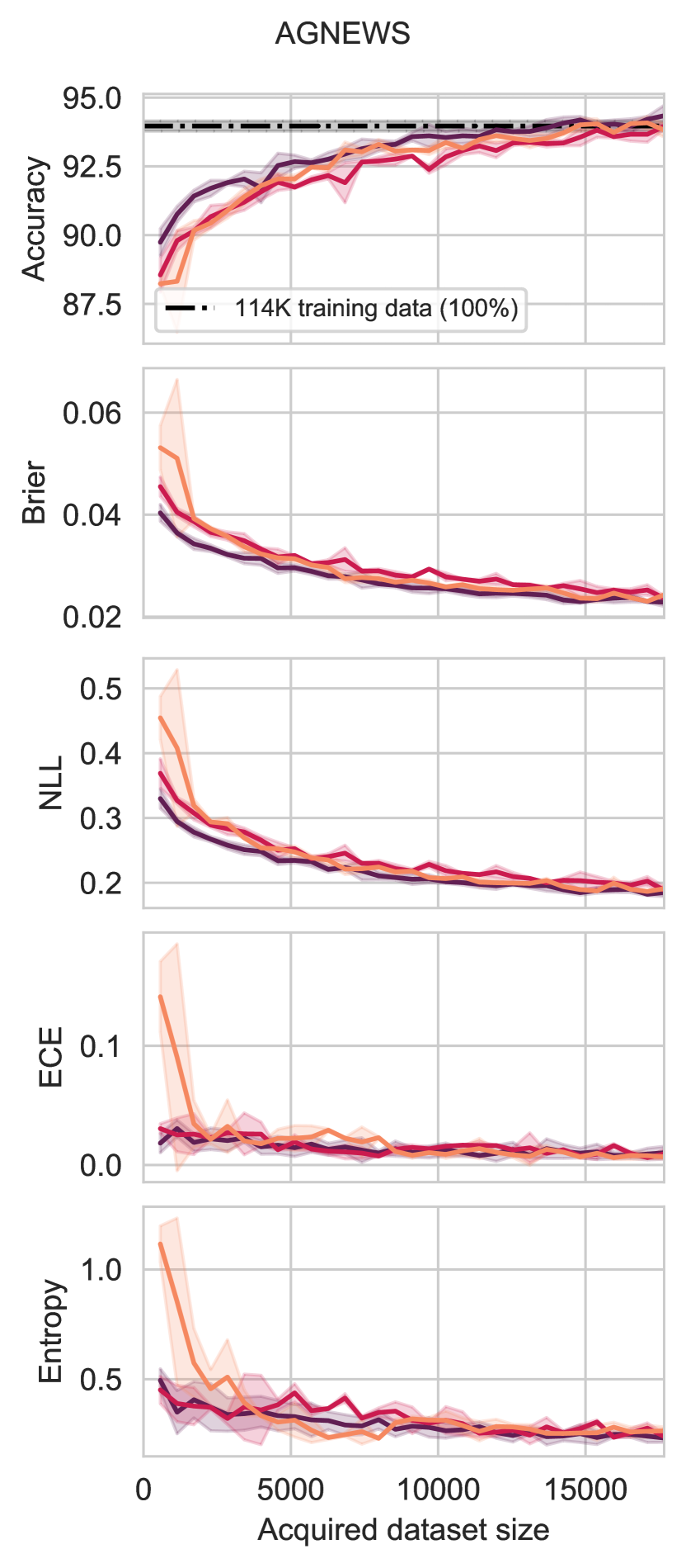
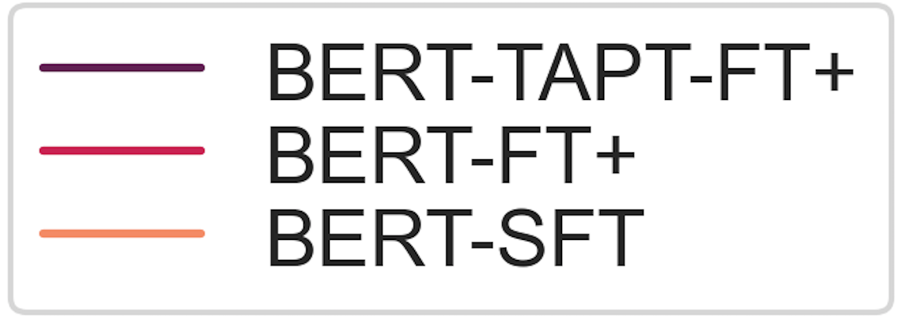
Figure 4: Ablation study for tapt and ft+.

5 Conclusion

We have presented a simple yet effective training scheme for AL with pretrained LMs that accounts for varying data availability and instability of fine-tuning. Specifically, we propose to first continue pretraining the LM with the available unlabeled data to adapt it to the task-specific domain. This way, we leverage not only the available labeled data at each AL iteration, but the entire unlabeled pool. We further propose a method to fine-tune the model during AL iterations so that training is robust in both low and high resource data settings.

Our experiments show that our approach yields substantially better results than standard fine-tuning in five standard NLP datasets. Furthermore, we find that the training strategy can be more important than the acquisition strategy. In other words, a poor training strategy can be a crucial impediment to the effectiveness of a good acquisition function, and thus limit its effectiveness (even over random sampling). Hence, our work highlights how critical it is to properly adapt a pretrained LM to the low data resource AL setting.

As state-of-the-art models in NLP advance rapidly, in the future we would be interested in exploring the use of larger LMs, such as Gpt-3 Brown et al. (2020) and Flan Wei et al. (2022). These models have achieved impressive performance in very low data resource settings (e.g. zero-shot and few-shot), so we would imagine they would be good candidates for the challenging setting of active learning.

Appendix A Appendix: Experimental Setup

A.1 Datasets

We experiment with five diverse natural language understanding tasks including binary and multi-class labels and varying dataset sizes (Table 1). The first task is question classification using the six-class version of the small trec-6 dataset of open-domain, fact-based questions divided into broad semantic categories Voorhees and Tice (2000). We also evaluate our approach on sentiment analysis using the binary movie review imdb dataset Maas et al. (2011) and the binary version of the sst-2 dataset Socher et al. (2013). We finally use the large-scale agnews and dbpedia datasets from  Zhang et al. (2015) for topic classification. We undersample the latter and form a $\mathcal{D}_{\textbf{pool}}$ of $20$K examples and $\mathcal{D}_{\textbf{val}}$ $2$K as in  Margatina et al. (2021). For trec-6, imdb and sst-2 we randomly sample $10\%$ from the training set to serve as the validation set, while for agnews we sample $5$%. For the dbpedia dataset we undersample both training and validation datasets (from the standard splits) to facilitate our AL simulation (i.e. the original dataset consists of $560$K training and $28$K validation data examples). For all datasets we use the standard test set, apart from the sst-2 dataset that is taken from the glue benchmark Wang et al. (2019) we use the development set as the held-out test set (and subsample a development set from the original training set).

A.2 Training & AL Details

We use BERT-base Devlin et al. (2019) and fine-tune it (tapt §2) for $100$K steps, with learning rate $2e-05$ and the rest of hyperparameters as in Gururangan et al. (2020) using the HuggingFace library Wolf et al. (2020). We evaluate the model $5$ times per epoch on $\mathcal{D}_{val}$ and keep the one with the lowest validation loss as in Dodge et al. (2020). We use the code provided by Kirsch et al. (2019) for the uncertainty-based acquisition functions and Yuan et al. (2020) for Alps, Badge and BertKM. We use the standard splits provided for all datasets, if available, otherwise we randomly sample a validation set. We test all models on a held-out test set. We repeat all experiments with five different random seeds resulting into different initializations of $\mathcal{D}_{\textbf{lab}}$ and the weights of the extra task-specific output feedforward layer. For all datasets we use as budget the $15\%$ of $\mathcal{D}_{\textbf{pool}}$. Each experiment is run on a single Nvidia Tesla V100 GPU.

A.3 Hyperparameters

For all datasets we train BERT-base Devlin et al. (2019) from the HuggingFace library Wolf et al. (2020) in Pytorch Paszke et al. (2019). We train all models with batch size $16$, learning rate $2e-5$, no weight decay, AdamW optimizer with epsilon $1e-8$. For all datasets we use maximum sequence length of $128$, except for imdb and agnews that contain longer input texts, where we use $256$. To ensure reproducibility and fair comparison between the various methods under evaluation, we run all experiments with the same five seeds that we randomly selected from the range $[1,9999]$.

A.4 Baselines

Acquisition functions

We compare Entropywith four baseline acquisition functions. The first is the standard AL baseline, Random, which applies uniform sampling and selects $k$ data points from $\mathcal{D}_{\textbf{pool}}$ at each iteration. The second is Badge Ash et al. (2020), an acquisition function that aims to combine diversity and uncertainty sampling. The algorithm computes gradient embeddings $g_{x}$ for every candidate data point $x$ in $\mathcal{D}_{\textbf{pool}}$ and then uses clustering to select a batch. Each $g_{x}$ is computed as the gradient of the cross-entropy loss with respect to the parameters of the model’s last layer. We also compare against a recently introduced cold-start acquisition function called Alps Yuan et al. (2020). Alps acquisition uses the masked language model (MLM) loss of Bert as a proxy for model uncertainty in the downstream classification task. Specifically, aiming to leverage both uncertainty and diversity, Alps forms a surprisal embedding $s_{x}$ for each $x$, by passing the unmasked input $x$ through the Bert MLM head to compute the cross-entropy loss for a random 15% subsample of tokens against the target labels. Alps clusters these embeddings to sample $k$ sentences for each AL iteration. Last, following Yuan et al. (2020), we use BertKM as a diversity baseline, where the $l_{2}$ normalized Bert output embeddings are used for clustering.

Models & Fine-tuning Methods

We evaluate two variants of the pretrained language model; the original Bert model, used in Yuan et al. (2020) and Ein-Dor et al. (2020), and our adapted model Bert-tapt (§2), and two fine-tuning methods; our proposed fine-tuning approach ft+ (§2) and standard Bert fine-tuning sft.

Model	trec-6	dbpedia	imdb	sst-2	agnews
Validation Set
bert	94.4	99.1	90.7	93.7	94.4
bert-tapt	95.2	99.2	91.9	94.3	94.5
Test Set
bert	80.6	99.2	91.0	90.6	94.0
bert-tapt	77.2	99.2	91.9	90.8	94.2

Table 2: Accuracy with $100\%$ of data over five runs (different random seeds).

Appendix B Appendix: Analysis

B.1 Task-Adaptive Pretraining (tapt) & Full-Dataset Performance

As discussed in §2 and §4, we continue training the BERT-base Devlin et al. (2019) pretrained masked language model using the available data $\mathcal{D}_{\textbf{pool}}$. We explored various learning rates between $1e-4$ and $1e-5$ and found the latter to produce the lowest validation loss. We trained each model (one for each dataset) for up to $100$K optimization steps, we evaluated on $\mathcal{D}_{\textbf{val}}$ every $500$ steps and saved the checkpoint with the lowest validation loss. We used the resulting model in our (Bert-tapt) experiments. We plot the learning curves of masked language modeling task (tapt) for three datasets and all considered learning rates in Figure 5. We notice that a smaller learning rate facilitates the training of the MLM.

In Table 2 we provide the validation and test accuracy of Bert and Bert-tapt for all datasets. We present the mean across runs with three random seeds. For fine-tuning the models, we used the proposed approach ft+ (§2).

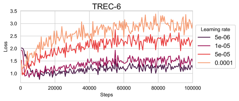
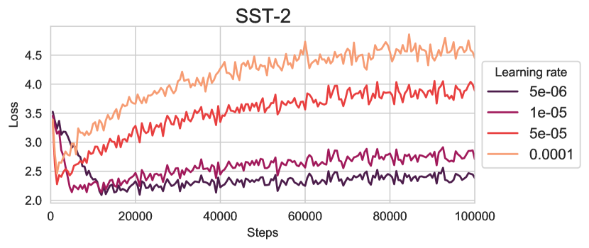
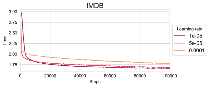
Figure 5: Learning curves of tapt for various learning rates.

	trec-6	sst-2	imdb	dbpedia	agnews
Random	0/0	0/0	0/0	0/0	0/0
Alps	0/57	0/478	0/206	0/134	0/634
Badge	0/63	0/23110	0/1059	0/192	-
BertKM	0/47	0/2297	0/324	0/137	0/3651
Entropy	81/0	989/0	557/0	264/0	2911/0
Least Confidence	69/0	865/0	522/0	256/0	2607/0
BALD	69/0	797/0	524/0	256/0	2589/0
BatchBALD	69/21	841/1141	450/104	256/482	2844/5611

Table 3: Runtimes (in seconds) for all datasets. In each cell of the table we present a tuple $i/s$ where $i$ is the inference time and $s$ the selection time. Inference time is the time for the model to perform a forward pass for all the unlabeled data in $\mathcal{D}_{\textbf{pool}}$ and selection time is the time that each acquisition function requires to rank all candidate data points and select $k$ for annotation (for a single iteration). Since we cannot report the runtimes for every model in the AL pipeline (at each iteration the size of $\mathcal{D}_{\textbf{pool}}$ changes), we provide the median.

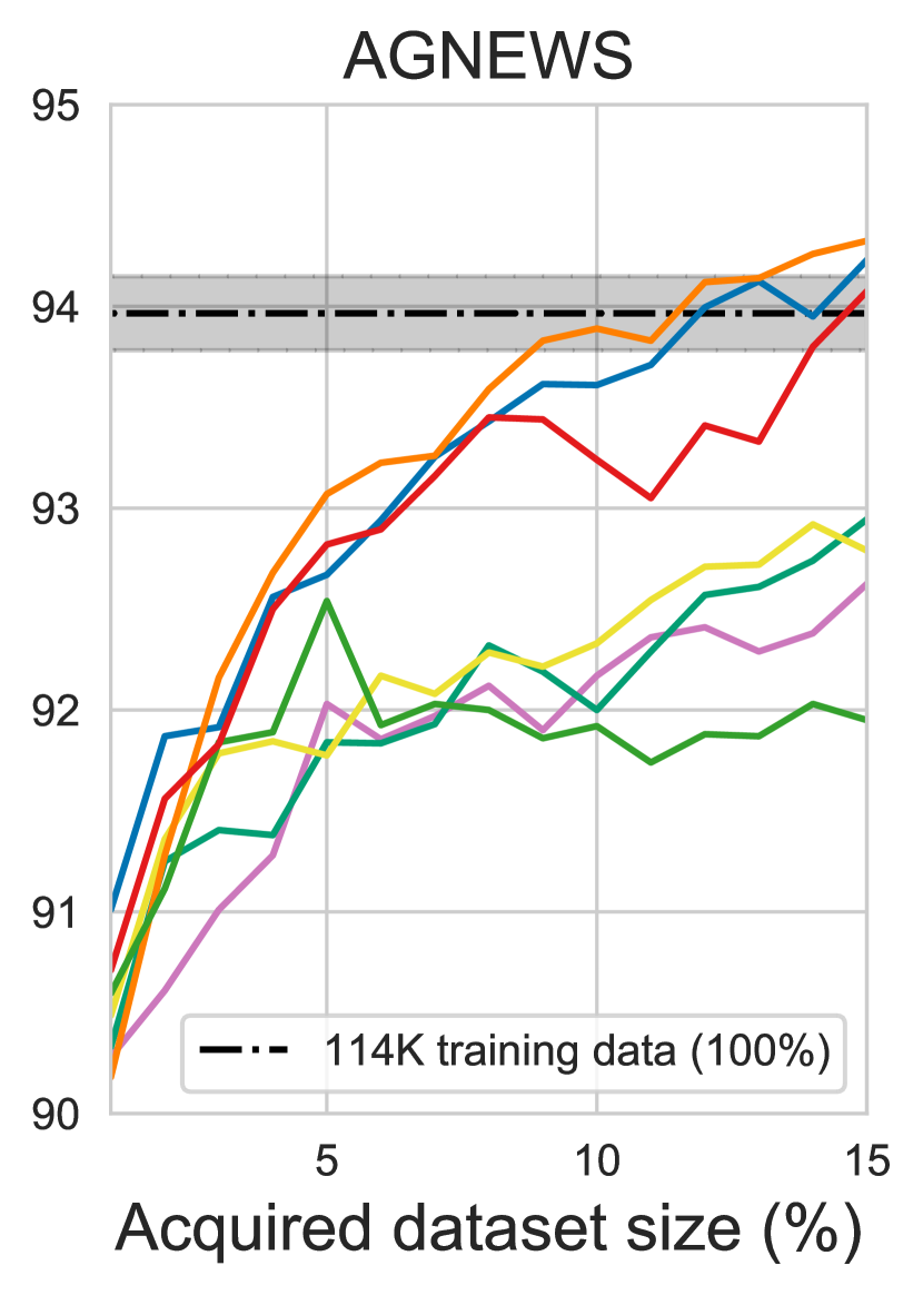
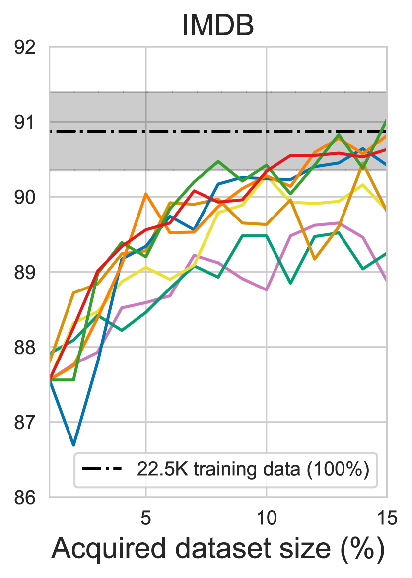
Figure 6: Comparison of acquisition functions using tapt and ft+ in training Bert.

B.2 Performance of Acquisition Functions

In our Bert-tapt-ft+ experiments so far, we showed results with Entropy. We have also experimented with various uncertainty-based acquisition functions. Specifically, four uncertainty-based acquisition functions are used in our work: Least Confidence, Entropy, BALD and BatchBALD. Least Confidence Lewis and Gale (1994) sorts $\mathcal{D}_{pool}$ by the probability of not predicting the most confident class, in descending order, Entropy Shannon (1948) selects samples that maximize the predictive entropy, and BALD Houlsby et al. (2011), short for Bayesian Active Learning by Disagreement, chooses data points that maximize the mutual information between predictions and model’s posterior probabilities. BatchBALD Kirsch et al. (2019) is a recently introduced extension of BALD that jointly scores points by estimating the mutual information between multiple data points and the model parameters. This iterative algorithm aims to find batches of informative data points, in contrast to BALD that chooses points that are informative individually. Note that Least Confidence, Entropy and BALD have been used in AL for NLP by Siddhant and Lipton (2018). To the best of our knowledge, BatchBALD is evaluated for the first time in the NLP domain.

Instead of using the output softmax probabilities for each class, we use a probabilistic formulation of deep neural networks in order to acquire better calibrated scores. Monte Carlo (MC) dropout Gal and Ghahramani (2016) is a simple yet effective method for performing approximate variational inference, based on dropout Srivastava et al. (2014). Gal and Ghahramani (2016) prove that by simply performing dropout during the forward pass in making predictions, the output is equivalent to the prediction when the parameters are sampled from a variational distribution of the true posterior. Therefore, dropout during inference results into obtaining predictions from different parts of the network. Our Bert-based $\mathcal{M}_{i}$ model uses dropout layers during training for regularization. We apply MC dropout by simply activating them during test time and we perform multiple stochastic forward passes. Formally, we do $N$ passes of every $x\in\mathcal{D}_{\textbf{pool}}$ through $\mathcal{M}_{i}(x;W_{i})$ to acquire $N$ different output probability distributions for each $x$. MC dropout for AL has been previously used in the literature Gal et al. (2017); Shen et al. (2017); Siddhant and Lipton (2018); Lowell and Lipton (2019); Ein-Dor et al. (2020); Shelmanov et al. (2021).

Our findings show that all functions provide similar performance, except for BALD that slightly underperforms. This makes our approach agnostic to the selected uncertainty-based acquisition method. We also evaluate our proposed methods with our baseline acquisition functions, i.e. Random, Alps, BertKM and Badge, since our training strategy is orthogonal to the acquisition strategy. We compare all acquisition functions with Bert-tapt-ft+ for agnews and imdb in Figure 6. We observe that in general uncertainty-based acquisition performs better compared to diversity, while all acquisition strategies have benefited from our training strategy (tapt and ft+).

B.3 Efficiency of Acquisition Functions

In this section we discuss the efficiency of the eight acquisition functions considered in this work; Random, Alps, Badge, BertKM, Entropy, Least Confidence, BALD and BatchBALD.

In Table 3 we provide the runtimes for all acquisition functions and datasets. Each AL experiments consists of multiple iterations and (therefore multiple models), each with a different training dataset $\mathcal{D}_{\textbf{lab}}$ and pool of unlabeled data $\mathcal{D}_{\textbf{pool}}$. In order to evaluate how computationally heavy is each method, we provide the median of all the models in one AL experiment. We calculate the runtime of two types of functionalities. The first is the inference time and stands for the forward pass of each $x\in\mathcal{D}_{\textbf{pool}}$ to acquire confidence scores for uncertainty sampling. Random, Alps, Badge and BertKM do not require this step so it is only applied of uncertainty-based acquisition where acquiring uncertainty estimates with MC dropout is needed. The second functionality is selection time and measures how much time each acquisition function requires to rank and select the $k$ data points from $\mathcal{D}_{\textbf{pool}}$ to be labeled in the next step of the AL pipeline. Random, Entropy, Least Confidence and BALD perform simple equations to rank the data points and therefore so do not require selection time. On the other hand, Alps, Badge, BertKM and BatchBALD perform iterative algorithms that increase selection time. From all acquisition functions Alps and BertKM are faster because they do not require the inference step of all the unlabeled data to the model. Entropy, Least Confidence and BALD require the same time for selecting data, which is equivalent for the time needed to perform one forward pass of the entire $\mathcal{D}_{\textbf{pool}}$. Finally Badge and BatchBALD are the most computationally heavy approaches, since both algorithms require multiple computations for the selection time. Random has a total runtime of zero seconds, as expected.

References

- Ash et al. (2020) Jordan T. Ash, Chicheng Zhang, Akshay Krishnamurthy, John Langford, and Alekh Agarwal. 2020. Deep batch active learning by diverse, uncertain gradient lower bounds. In International Conference on Learning Representations.
- Bodó et al. (2011) Zalán Bodó, Zsolt Minier, and Lehel Csató. 2011. Active learning with clustering. In Proceedings of the Active Learning and Experimental Design workshop In conjunction with AISTATS 2010, volume 16, pages 127–139.
- Brinker (2003) Klaus Brinker. 2003. Incorporating diversity in active learning with support vector machines. In Proceedings of the International Conference on Machine Learning, pages 59–66.
- Brown et al. (2020) Tom Brown, Benjamin Mann, Nick Ryder, Melanie Subbiah, Jared D Kaplan, Prafulla Dhariwal, Arvind Neelakantan, Pranav Shyam, Girish Sastry, Amanda Askell, Sandhini Agarwal, Ariel Herbert-Voss, Gretchen Krueger, Tom Henighan, Rewon Child, Aditya Ramesh, Daniel Ziegler, Jeffrey Wu, Clemens Winter, Chris Hesse, Mark Chen, Eric Sigler, Mateusz Litwin, Scott Gray, Benjamin Chess, Jack Clark, Christopher Berner, Sam McCandlish, Alec Radford, Ilya Sutskever, and Dario Amodei. 2020. Language models are few-shot learners. In Advances in Neural Information Processing Systems, volume 33, pages 1877–1901. Curran Associates, Inc.
- Cohn et al. (1996) David A. Cohn, Zoubin Ghahramani, and Michael I. Jordan. 1996. Active learning with statistical models. Journal of Artificial Intelligence Research, 4(1):129–145.
- Devlin et al. (2019) Jacob Devlin, Ming-Wei Chang, Kenton Lee, and Kristina Toutanova. 2019. BERT: Pre-training of deep bidirectional transformers for language understanding. In Proceedings of the Conference of the North American Chapter of the Association for Computational Linguistics: Human Language Technologies, pages 4171–4186.
- Dodge et al. (2020) Jesse Dodge, Gabriel Ilharco, Roy Schwartz, Ali Farhadi, Hannaneh Hajishirzi, and Noah A. Smith. 2020. Fine-tuning pretrained language models: Weight initializations, data orders, and early stopping. ArXiv.
- Ducoffe and Precioso (2018) Melanie Ducoffe and Frederic Precioso. 2018. Adversarial active learning for deep networks: a margin based approach.
- Ein-Dor et al. (2020) Liat Ein-Dor, Alon Halfon, Ariel Gera, Eyal Shnarch, Lena Dankin, Leshem Choshen, Marina Danilevsky, Ranit Aharonov, Yoav Katz, and Noam Slonim. 2020. Active learning for BERT: An empirical study. In Proceedings of theConference on Empirical Methods in Natural Language Processing, pages 7949–7962.
- Gal and Ghahramani (2016) Yarin Gal and Zoubin Ghahramani. 2016. Dropout as a bayesian approximation: Representing model uncertainty in deep learning. In Proceedings of the International Conference on Machine Learning, volume 48, pages 1050–1059.
- Gal et al. (2017) Yarin Gal, Riashat Islam, and Zoubin Ghahramani. 2017. Deep Bayesian active learning with image data. In Proceedings of the International Conference on Machine Learning, volume 70, pages 1183–1192.
- Gururangan et al. (2020) Suchin Gururangan, Ana Marasović, Swabha Swayamdipta, Kyle Lo, Iz Beltagy, Doug Downey, and Noah A. Smith. 2020. Don’t stop pretraining: Adapt language models to domains and tasks. In Proceedings of the 58th Annual Meeting of the Association for Computational Linguistics, pages 8342–8360, Online. Association for Computational Linguistics.
- Houlsby et al. (2011) Neil Houlsby, Ferenc Huszár, Zoubin Ghahramani, and Máté Lengyel. 2011. Bayesian active learning for classification and preference learning. ArXiv.
- Howard and Ruder (2018) Jeremy Howard and Sebastian Ruder. 2018. Universal language model fine-tuning for text classification. In Proceedings of the Annual Meeting of the Association for Computational Linguistics, pages 328–339.
- Ikhwantri et al. (2018) Fariz Ikhwantri, Samuel Louvan, Kemal Kurniawan, Bagas Abisena, Valdi Rachman, Alfan Farizki Wicaksono, and Rahmad Mahendra. 2018. Multi-task active learning for neural semantic role labeling on low resource conversational corpus. In Proceedings of the Workshop on Deep Learning Approaches for Low-Resource NLP, pages 43–50.
- Karamcheti et al. (2021) Siddharth Karamcheti, Ranjay Krishna, Li Fei-Fei, and Christopher Manning. 2021. Mind your outliers! investigating the negative impact of outliers on active learning for visual question answering. In Proceedings of the 59th Annual Meeting of the Association for Computational Linguistics and the 11th International Joint Conference on Natural Language Processing (Volume 1: Long Papers), pages 7265–7281, Online. Association for Computational Linguistics.
- Kasai et al. (2019) Jungo Kasai, Kun Qian, Sairam Gurajada, Yunyao Li, and Lucian Popa. 2019. Low-resource deep entity resolution with transfer and active learning. In Proceedings of the Conference of the Association for Computational Linguistic, pages 5851–5861.
- Kirsch et al. (2019) Andreas Kirsch, Joost van Amersfoort, and Yarin Gal. 2019. BatchBALD: Efficient and diverse batch acquisition for deep bayesian active learning. In Neural Information Processing Systems, pages 7026–7037.
- Lewis and Gale (1994) David D. Lewis and William A. Gale. 1994. A sequential algorithm for training text classifiers. In In Proceedings of the Annual International ACM SIGIR Conference on Research and Development in Information Retrieval.
- Liu et al. (2020) Yinhan Liu, Myle Ott, Naman Goyal, Jingfei Du, Mandar Joshi, Danqi Chen, Omer Levy, Mike Lewis, Luke Zettlemoyer, and Veselin Stoyanov. 2020. Ro{bert}a: A robustly optimized {bert} pretraining approach.
- Loshchilov and Hutter (2019) Ilya Loshchilov and Frank Hutter. 2019. Decoupled weight decay regularization. In International Conference on Learning Representations.
- Lowell and Lipton (2019) David Lowell and Zachary C Lipton. 2019. Practical obstacles to deploying active learning. Proceedings of the Conference on Empirical Methods in Natural Language Processing and the International Joint Conference on Natural Language Processing, pages 21–30.
- Maas et al. (2011) Andrew L. Maas, Raymond E. Daly, Peter T. Pham, Dan Huang, Andrew Y. Ng, and Christopher Potts. 2011. Learning word vectors for sentiment analysis. In Proceedings of the Annual Meeting of the Association for Computational Linguistics: Human Language Technologies, pages 142–150.
- Margatina et al. (2021) Katerina Margatina, Giorgos Vernikos, Loïc Barrault, and Nikolaos Aletras. 2021. Active learning by acquiring contrastive examples. In Proceedings of the 2021 Conference on Empirical Methods in Natural Language Processing, pages 650–663, Online and Punta Cana, Dominican Republic. Association for Computational Linguistics.
- Mosbach et al. (2021) Marius Mosbach, Maksym Andriushchenko, and Dietrich Klakow. 2021. On the stability of fine-tuning {bert}: Misconceptions, explanations, and strong baselines. In International Conference on Learning Representations.
- Ovadia et al. (2019) Yaniv Ovadia, Emily Fertig, Jie Ren, Zachary Nado, D. Sculley, Sebastian Nowozin, Joshua Dillon, Balaji Lakshminarayanan, and Jasper Snoek. 2019. Can you trust your model's uncertainty? evaluating predictive uncertainty under dataset shift. In Advances in Neural Information Processing Systems, volume 32, pages 13991–14002.
- Paszke et al. (2019) Adam Paszke, Sam Gross, Francisco Massa, Adam Lerer, James Bradbury, Gregory Chanan, Trevor Killeen, Zeming Lin, Natalia Gimelshein, Luca Antiga, Alban Desmaison, Andreas Kopf, Edward Yang, Zachary DeVito, Martin Raison, Alykhan Tejani, Sasank Chilamkurthy, Benoit Steiner, Lu Fang, Junjie Bai, and Soumith Chintala. 2019. Pytorch: An imperative style, high-performance deep learning library. In Advances in Neural Information Processing Systems, pages 8024–8035.
- Prabhu et al. (2019) Ameya Prabhu, Charles Dognin, and Maneesh Singh. 2019. Sampling bias in deep active classification: An empirical study. In Proceedings of the Conference on Empirical Methods in Natural Language Processing and the International Joint Conference on Natural Language Processing, pages 4056–4066.
- Sener and Savarese (2018) Ozan Sener and Silvio Savarese. 2018. Active learning for convolutional neural networks: A core-set approach. In International Conference on Learning Representations.
- Settles (2009) Burr Settles. 2009. Active learning literature survey. Computer sciences technical report.
- Shannon (1948) Claude Elwood Shannon. 1948. A mathematical theory of communication. The Bell System Technical Journal.
- Shelmanov et al. (2021) Artem Shelmanov, Dmitri Puzyrev, Lyubov Kupriyanova, Denis Belyakov, Daniil Larionov, Nikita Khromov, Olga Kozlova, Ekaterina Artemova, Dmitry V. Dylov, and Alexander Panchenko. 2021. Active learning for sequence tagging with deep pre-trained models and Bayesian uncertainty estimates. In Proceedings of the 16th Conference of the European Chapter of the Association for Computational Linguistics: Main Volume, pages 1698–1712, Online. Association for Computational Linguistics.
- Shen et al. (2017) Yanyao Shen, Hyokun Yun, Zachary Lipton, Yakov Kronrod, and Animashree Anandkumar. 2017. Deep active learning for named entity recognition. In Proceedings of the Workshop on Representation Learning for NLP, pages 252–256.
- Siddhant and Lipton (2018) Aditya Siddhant and Zachary C Lipton. 2018. Deep bayesian active learning for natural language processing: Results of a Large-Scale empirical study. In Proceedings of the Conference on Empirical Methods in Natural Language Processing, pages 2904–2909.
- Socher et al. (2013) Richard Socher, Alex Perelygin, Jean Wu, Jason Chuang, Christopher D. Manning, Andrew Ng, and Christopher Potts. 2013. Recursive deep models for semantic compositionality over a sentiment treebank. In Proceedings of the Conference on Empirical Methods in Natural Language Processing, pages 1631–1642.
- Srivastava et al. (2014) N Srivastava, G Hinton, A Krizhevsky, and others. 2014. Dropout: a simple way to prevent neural networks from overfitting. Journal of Machine Learning Research, 15(56):1929–1958.
- Voorhees and Tice (2000) Ellen Voorhees and Dawn Tice. 2000. The trec-8 question answering track evaluation. Proceedings of the Text Retrieval Conference.
- Wang et al. (2019) Alex Wang, Amanpreet Singh, Julian Michael, Felix Hill, Omer Levy, and Samuel R. Bowman. 2019. GLUE: A multi-task benchmark and analysis platform for natural language understanding. In International Conference on Learning Representations.
- Wei et al. (2022) Jason Wei, Maarten Bosma, Vincent Zhao, Kelvin Guu, Adams Wei Yu, Brian Lester, Nan Du, Andrew M. Dai, and Quoc V Le. 2022. Finetuned language models are zero-shot learners. In International Conference on Learning Representations.
- Wolf et al. (2020) Thomas Wolf, Lysandre Debut, Victor Sanh, Julien Chaumond, Clement Delangue, Anthony Moi, Pierric Cistac, Tim Rault, Remi Louf, Morgan Funtowicz, Joe Davison, Sam Shleifer, Patrick von Platen, Clara Ma, Yacine Jernite, Julien Plu, Canwen Xu, Teven Le Scao, Sylvain Gugger, Mariama Drame, Quentin Lhoest, and Alexander Rush. 2020. Transformers: State-of-the-art natural language processing. In Proceedings of the Conference on Empirical Methods in Natural Language Processing: System Demonstrations, pages 38–45.
- Yuan et al. (2020) Michelle Yuan, Hsuan-Tien Lin, and Jordan Boyd-Graber. 2020. Cold-start active learning through self-supervised language modeling.
- Zhang and Plank (2021) Mike Zhang and Barbara Plank. 2021. Cartography active learning. In Findings of the Association for Computational Linguistics: EMNLP 2021, pages 395–406, Punta Cana, Dominican Republic. Association for Computational Linguistics.
- Zhang et al. (2020) Tianyi Zhang, Felix Wu, Arzoo Katiyar, Kilian Q. Weinberger, and Yoav Artzi. 2020. Revisiting few-sample bert fine-tuning. ArXiv.
- Zhang et al. (2015) Xiang Zhang, Junbo Zhao, and Yann LeCun. 2015. Character-level convolutional networks for text classification. In Advances in Neural Information Processing Systems, volume 28, pages 649–657. Curran Associates, Inc.