Better Latent Spaces for Better Autoencoders

Barry M. Dillon¹, Tilman Plehn¹, Christof Sauer², and Peter Sorrenson³,

Abstract

Autoencoders as tools behind anomaly searches at the LHC have the structural problem that they only work in one direction, extracting jets with higher complexity but not the other way around. To address this, we derive classifiers from the latent space of (variational) autoencoders, specifically in Gaussian mixture and Dirichlet latent spaces. In particular, the Dirichlet setup solves the problem and improves both the performance and the interpretability of the networks.

 

Content

1. 1 Introduction
2. 2 The problem with autoencoding jets
3. 3 Gaussian-Mixture-VAE
4. 4 Dirichlet-VAE
5. 5 Outlook
6. A Unsupervised Lund plane

 

1 Introduction

If new physics exists at the scales currently probed at the LHC, then it is more elusive than expected and could be difficult to uncover with traditional means and without a significant increase in the number of analyses. It is here that unsupervised machine learning techniques can play a crucial role, not fulfilled by traditional, signal-driven search techniques.

Autoencoders (AEs) with a bottleneck are the simplest unsupervised machine learning tool. They are built on a network which maps a high-dimensional data representation onto itself, constructing a typical or average object. The goal is to reconstruct the input data as accurately as possible. If we then compress a set of layers in the middle of this network, we cut into its expressiveness, such that atypical objects cannot be related to the learned output any longer. In early high-energy physics works, AEs have been shown to classify between anomalous jets and QCD jets using the reconstruction error as the classifier [1, 2, 3, 4].

In a more sophisticated manner, variational autoencoders [5] (VAEs) add structure to the bottleneck. In a first, encoding step, the high-dimensional data representation is mapped to a lower-dimensional latent distribution; next, the decoder learns a model to generate the input data by sampling from this latent distribution. After training, the latent space should contain information about each instance of the data-set that is not apparent in the high-dimensional input representation. At the LHC, it is possible to use this latent space representation of the jets for classification [6, 7, 8], and even anomaly detection. The use of machine learning methods for anomaly detection has received a lot of attention in recent years [9, 10, 11, 12, 13, 14, 15, 16, 17, 18, 19, 20, 21], including a first ATLAS analysis [22], and the LHC Olympics 2020 community challenge has seen many groups submit their results on a di-jet anomaly search using black-box data-sets [23]. Additional papers studying similar unsupervised LHC problems include Ref. [24, 25, 26, 27, 28, 29, 30, 31, 32, 33, 34, 35, 36, 37, 38, 39, 40].

While (V)AE-analyses based directly on anomaly scores appear unrealistic, they allow us to collect and analyse data in a more targeted manner, for instance as part of the trigger, in addition to pre-scaling, or complementing minimum bias events. This kind of application is fundamentally different from weakly supervised analyses, which are based on some kind of signal hypotheses or expected signal features [41]. As a matter of fact, the statistical nature of LHC data will typically turn supervised techniques into weakly supervised analyses the moment we train on data rather than Monte Carlos. In the spirit of anomaly searches, we are studying unsupervised learning of QCD and top jets in this paper. The question is how a VAE can encode something related to a class label in the latent space, and how more structured latent space geometries help with unsupervised classification.

We start in Section 2 by demonstrating how AEs and VAEs perform when using the compressed/latent space representations for unsupervised jet classification. We then study a generalisation, in which the Gaussian prior is replaced by a Gaussian-Mixture prior (GMVAE) [42, 43, 44, 45, 46, 47, 48] in Section 3. In Section 4 we introduce the Dirichlet-VAE (DVAE), which uses a compact latent space with a Dirichlet prior [49, 50]. Through a specific choice of decoder architecture we can interpret the decoder weights as the parameters of the mixture distributions in the probabilistic model, and can visualise these to directly interpret what the neural network is learning. Our technique shares similarities with topic-modelling approaches [51, 52, 11, 12, 53]. We present our conclusions in Section 5.

2 The problem with autoencoding jets

While autoencoders have been proposed for unsupervised jet classification [1, 2], they are known to be problematic in general applications. We briefly discuss their issues and possible improvements through VAEs, and motivate our new approach based on appropriately chosen latent spaces.

Jet images and data set

Throughout the paper we use the QCD and top jet samples generated for the community top-tagging challenge outlined in Ref. [54], in the same jet image representation as in our earlier AE study [1]. We simulate the jets with Pythia8 [55] (default tune) using a center-of-mass energy of 14 TeV and ignoring pile-up and multi-parton interactions. We use Delphes [56] for a fast detector simulation with the default ATLAS detector card. The jets are defined through the anti-$k_{T}$ algorithm [57, 58] in FastJet [59] with a radius of $R=0.8$. In each event we kept only the leading jet and only if $p_{T}=550~{}...~{}650$ GeV and $|\eta|<2$. Additionally, we require top jets to be matched to a parton-level top within the jet radius and all parton-level decay products to lay within the jet radius. To define the jet constituents we use the Delphes energy-flow algorithm and keep the leading 200 constituents from each jet for the analysis, while zero-padding the empty entries. We do not include particle ID or tracking information.

For the pre-processing of the jets we follow a procedure similar to Refs. [1, 60]. We do the pre-processing at the level of the jet constituents, prior to pixelization. First, we center the jet using the $k_{T}$-weighted centroid of the jet constituents, such that the major principle axis points upwards. We then flip the image in both axes so that most of the $p_{T}$ is located in the lower left quadrant. Once this is done we pixelize the image into a 40 by 40 array, with the intensity defined by the $p_{T}$ sum of the constituents per pixel. The pixel sizes are $[\Delta\eta,\Delta\phi]=[0.029,0.035$] and during pixelization we crop the image to reduce the sparsity of the information within it. In Fig. 1 we show the average of 10k QCD and top jet images after the pre-processing has been applied.

Our data-set consists of 100k QCD jets and 100k top jets, and in each analysis we use the maximum number of jets possible. For example if we want equal numbers of QCD and top jets we use 100k of each, and if we want a data-set where the QCD jets are being treated as the background and the number of top jets is varied, we keep the full 100k QCD jets and vary the number of top jets. For all presented results we use a 90/10 split of the data for training and testing. The data samples are shuffled and the testing data is selected randomly on each run.

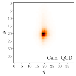
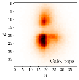
Figure 1: Average of 100k QCD and top jet images after pre-processing.

The networks

Both the AE and the VAE consist of two networks illustrated in Fig. 2; an encoder and a decoder. In the case of the AE the encoder maps the data to a so-called bottleneck, for instance an $n$-dimensional vector $z$. In the case of the VAE the encoder maps the data to a posterior distribution, which in this section is taken to be a Gaussian with diagonal covariance. This structures the encoder output and defines the latent space. An $n$-dimensional Gaussian latent space $z$ can be described by $2n$ numbers, $n$ means $\mu_{i}$ and $n$ log-variances $\log\sigma_{i}$. So that the network can be optimised through back-propagation we must be able to differentiate this sampling function with respect to the parameters of the posterior distribution. A re-parametrization of the sampling step [5] uses a vector of random numbers $\epsilon$ from an $n$-dimensional unit Gaussian, and then defines the sampled latent vector as $z=\mu+\sigma\odot\epsilon$. The Hadamard product $\odot$ implies the element-wise product of the two operands. The autoencoder loss used is the mean squared error

$$\mathcal{L}=\Big{\langle}\frac{1}{2}\lVert x-x^{\prime}\rVert^{2}\Big{\rangle}_{p_{\text{data}}(x)}\;,$$ (1)

where $x^{\prime}$ is the reconstruction of the input jet images $x$. The VAE loss function [5] has the form

$$\mathcal{L}=\Big{\langle}-\big{\langle}\log p_{\theta}(x|z)\big{\rangle}_{q_{\phi}(z|x)}+\beta_{\text{KL}}D_{\text{KL}}(q_{\phi}(z|x),p(z))\Big{\rangle}_{p_{\text{data}}(x)}\;,$$ (2)

with a learnable variational encoder $q_{\phi}(z|x)$ and decoder $p_{\theta}(x|z)$, where $\phi$ and $\theta$ represent the parameters of the encoder and decoder respectively. The $\beta_{\text{KL}}$ term allows us to control the relative influence of the reconstruction (first term) and latent loss (second term) in the gradient updates. We use the mean squared error of equation 1 as reconstruction loss, following from a choice of Gaussian $p_{\theta}(x|z)$. For the choice of standard normal $p(z)$, the KL divergence term has the following analytical form,

$$D_{\text{KL}}(q_{\phi}(z|x),p(z))=\frac{1}{2}\sum_{i=1}^{n}\left(\sigma_{i}^{2}+\mu_{i}^{2}-1-\log\sigma_{i}^{2}\right),$$ (3)

where $\sigma_{i}$ and $\mu_{i}$ are the outputs of the encoder for a given $x$. We set $\beta_{KL}=10^{-4}$ as we find that this gives us optimal results. For both the AE and the VAE the output layer of the decoder has a linear activation. The hidden layers of the encoder and decoder architectures in both cases use convolutional layers. All our neural network models are constructed and optimised with Tensorflow [61] and Keras [62], and all use the Adam optimiser [63] with a learning rate of $0.001$.

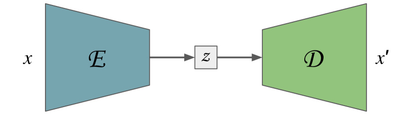
(a) AE setup

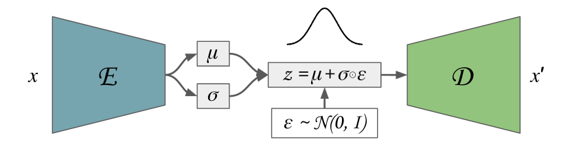
(b) VAE setup

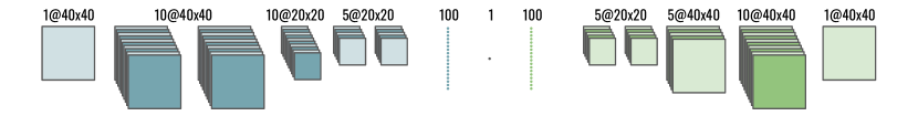
(c) Encoder and decoder

Figure 2: Architectures used for the AE and VAE networks in this study. All convolutions use a 5x5 kernel size and all layers use PReLU activations. Downsampling from 40x40 to 20x20 is achieved by average pooling, while upsampling is nearest neighbor interpolation.

Reconstruction-loss tagging

In the AE architecture the encoder compresses the input data into a bottleneck, encoding each instance of the data-set in a representation with a dimension much smaller than the dimension of the input data. The decoder then attempts to reconstruct the input data from the limited information encoded in the bottleneck. The idea behind the anomaly search is that the AE learns to compress and reconstruct the training data very well, but different unseen data passed through the trained AE will result in a large reconstruction error, or loss. In this way the AE may be used to search for data which is very different to the training data, or even data which is part of the training data but forms a small subclass of anomalous instances. This strategy fails for example in the case of QCD vs top jets, where the QCD jets are assumed to be anomalous [1]. The reason appears to be that the AE can encode simpler data with less features more easily, so if the anomalous data is structurally simpler than the dominant class, the AE with its reconstruction loss as the classification metric fails. A formal study of the limitations of AEs has been presented recently [64]. In Ref. [1] the results appeared insensitive to pre-processing, which can be explained by only the top jets being sensitive to the pre-processing in a significant way. Because the QCD jets mostly have just a single prong, the centering of the jets is the most relevant step.

Latent-space tagging

The AE drawbacks can be avoided through using an alternative classification metric to the reconstruction error. In the context of VAEs, the natural choice is to derive a metric from the latent space embedding [7, 8]. In this paper we study the behaviour of such metrics systematically and provide better-suited latent spaces.

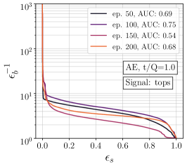
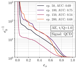
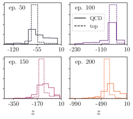
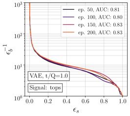
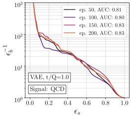
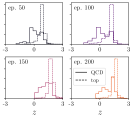
Figure 3: Results for the 1D AE (top) and VAE (bottom). In the large panels we show the ROC curves for tagging top and QCD as signal. In the small panels we show the distributions of the top and QCD jets in the bottleneck or latent space developed over the training.

For illustration purposes, we start with a 1D bottleneck for the AE and a 1D latent space for the VAE. One of our main points will be that the architecture of the network, in particular the latent space, plays an important role in determining the type of information learned by the network. It has been shown [2, 1] that with large bottlenecks of around 30 nodes it is possible to reconstruct $40\times 40$ jet images with good accuracy, while at the same time achieving reasonable top-tagging performance using the reconstruction error. In these cases, the latent space is unequivocally not a good classifier for top jets because the bottleneck is too large. With a bottleneck of this size the network can accurately encode kinematic information about each individual jet, allowing for an accurate per-jet reconstruction. The trouble is that this kinematic information encoded in the bottleneck does not tell us anything about the class the jet belongs to, i.e. top jet or QCD jet. To learn this information the network needs to learn how to reconstruct classes of jets, rather than individual jets. And to force the network to do this, we restrict the amount of information that can be encoded in the bottleneck. In the case of the VAE this has a nice probabilistic interpretation, since the mapping to the encoded space is performed by the posterior distribution $q(z|x)$. In 1D then the latent variable $z$ can be thought of as a continuous generalisation of a class label.

We are interested in three aspects of the (V)AE classifiers: (i) performance as a top-tagger, (ii) performance as a QCD-tagger, (iii) stable encoding in the latent space. To start, we restrict ourselves to samples with equal numbers of 100k top and QCD jets. We follow the evolution of the loss and find that all models converge before epoch 200. The results for the AE and the VAE are shown in Fig. 3. We immediately see that the AE bottleneck is not a robust classifier; the classification is unstable and the encoding in the bottleneck continues to evolve even after the loss function has converged. In the VAE plots we can see that the regularisation of the latent space has a positive effect. The latent space of the VAE is much more stable and structured than the AE bottleneck, even converging to a representation in which the top jets are almost clustered away from the QCD jets.

On the other hand, it is reasonable to assume that the most natural latent representation for a data-set such as ours would be one which naturally allows for a bi-modal structure. By construction, this is not achieved by the VAE with its unimodal Gaussian prior.

3 Gaussian-Mixture-VAE

While the standard VAE prior shapes a Gaussian latent space with a single mode, a symmetric anomaly search would prefer a dual-mode latent space to capture two classes of data. We introduce a Gaussian mixture prior, consisting of two mixture components or modes, and show how it performs on the benchmark from the previous section with balanced classes. We approximate the KL divergence between the Gaussian mixture prior and the latent representation of the events using a Monte Carlo estimate. There are papers using a Gaussian mixture as the VAE prior [43, 44, 45, 46], but most implementations are more complicated than ours, requiring additional inference networks, as the authors wish to calculate an analytical Kullback-Leibler (KL) divergence. In the most similar model to ours [47] the authors use an approximation to the KL-term [48] rather than a Monte Carlo estimate.

Gaussian mixture prior

We impose a Gaussian mixture prior on the $n$-dimensional latent space, where the Gaussian in each mixture has diagonal covariance. Such a model has the following conditional likelihood

$$p(z|r)=\prod_{i=1}^{n}\;\frac{1}{\sqrt{2\pi}\sigma_{r,i}}\;\exp\left(-\frac{(z_{i}-\mu_{r,i})^{2}}{2\sigma^{2}_{r,i}}\right)$$ (4)

where $\mu_{r,i}$ is the mean of mixture component $r=1~{}...~{}R$ in dimension $i$, and $\sigma^{2}_{r,i}$ is the corresponding variance. The prior is then simply calculated as $p(z)=\sum_{r}p(z|r)p(r)$, with $p(r)$ being the weight of mixture component $r$.

We allow all means, variances, and mixture weights to be learned. The means are learned as a $R\times n$ matrix $M$, the log variances as a $R\times n$ matrix $V$, and the unnormalized log mixture weights as a vector $a$ of length $R$. Since the mixture weights must be positive and sum to one, we apply the softmax operation,

$$p(r)=\frac{e^{a_{r}}}{\sum_{r^{\prime}}e^{a_{r^{\prime}}}}\;.$$ (5)

With this notation, we can rewrite the conditional likelihood as

$$p(z|r)=\prod_{i=1}^{n}\;\frac{1}{\sqrt{2\pi e^{V_{ri}}}}\;\exp\left(-\frac{(z_{i}-M_{ri})^{2}}{2e^{V_{ri}}}\right).$$ (6)

We can write this in log form,

$$\log\left(p(z|r)p(r)\right)=\sum_{i=1}^{n}\left(-\frac{(z_{i}-M_{ri})^{2}}{2e^{V_{ri}}}-\frac{1}{2}V_{ri}\right)-\frac{n}{2}\log(2\pi)+\log\text{softmax}(a_{r})\;,$$ (7)

from which we can apply the log-sum-exp operation to obtain the prior log-likelihood, $\log p(z)=\log\sum_{r}\exp\log(p(z|r)p(r))$. In our experiments we always chose $R=2$.

Mode-separation loss

As in a standard VAE, the GMVAE illustrated in Fig. 4 minimizes the negative ELBO loss,

$$\mathcal{L}=\Big{\langle}-\big{\langle}\log p_{\theta}(x|z)\big{\rangle}_{q_{\phi}(z|x)}+\beta_{\text{KL}}D_{\text{KL}}(q_{\phi}(z|x),p(z))\Big{\rangle}_{p_{\text{data}}(x)}\;,$$ (8)

with a learnable variational encoder $q_{\phi}(z|x)$ and decoder $p_{\theta}(x|z)$, where $\phi$ and $\theta$ represent the parameters of the encoder and decoder, respectively. The data-set consisting of a mixture of QCD and top jets here is indicated by $x$. The $\beta_{\text{KL}}$ term allows us to control the relative influence of the reconstruction and latent loss terms in the gradient updates. Exactly as was done for the VAE and AE, we use the mean squared error for the reconstruction loss and set $\beta_{KL}=10^{-4}$.

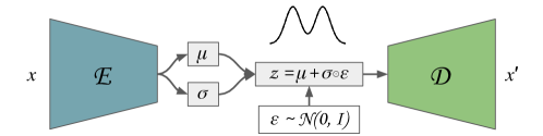
Figure 4: Architecture used for the GMVAE. The encoder and decoder are the same as for the (V)AE shown in Fig. 2(c). In contrast to the standard VAE, the prior distribution is learnable and can be bimodal.

The first term in Eq.(8) is treated in the standard way as a reconstruction loss, where a single sample is drawn from $q_{\phi}(z|x)$ to estimate the expectation. The second term comes with the challenge that for a Gaussian mixture we cannot calculate the KL-divergence analytically anymore. We instead estimate it using Monte Carlo samples [42] and start by re-writing it as

$$D_{\text{KL}}(q_{\phi}(z|x),p(z))=\big{\langle}\log q_{\phi}(z|x)\big{\rangle}_{q_{\phi}(z|x)}-\big{\langle}\log p(z)\big{\rangle}_{q_{\phi}(z|x)}\;.$$ (9)

The first contribution is the negative entropy of a Gaussian, which has the analytical form

$$\big{\langle}\log q_{\phi}(z|x)\big{\rangle}_{q_{\phi}(z|x)}=-\frac{n}{2}(1+\log(2\pi))-\frac{1}{2}\sum_{i=1}^{n}\log\sigma^{2}_{i}\;.$$ (10)

The second contribution to $D_{\text{KL}}$ can be estimated by a single Monte Carlo sample from $q_{\phi}(z|x)$, as in the reconstruction term, using the log-likelihood of the imposed prior derived in Eq.(7).

In testing this two-component mixture prior we observe that the mixture components collapse onto a single mode. To prevent this, we add a repulsive force between the modes, calculated as a function of the Ashman distance [65]. The Ashman-$D$ between two Gaussian distributions in one dimension is

$$D^{2}=\frac{2(\mu_{1}-\mu_{2})^{2}}{\sigma^{2}_{1}+\sigma^{2}_{2}}\;.$$ (11)

A value of $D>2$ indicates a clear mode separation. The distance can be extended to two $n$-dimensional Gaussians with diagonal covariance matrices as

$$D^{2}=\sum_{i=1}^{n}\frac{2(\mu_{1i}-\mu_{2i})^{2}}{\sigma^{2}_{1i}+\sigma^{2}_{2i}}\;,$$ (12)

where again $D>2$ indicates clear separation. We encourage bi-modality in our latent space by adding the loss term

$$\mathcal{L}_{A}=-\lambda_{A}\tanh\frac{D}{2}\;.$$ (13)

The tanh function eventually saturates and stops pushing apart the modes.

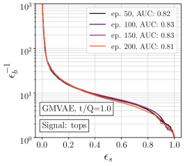
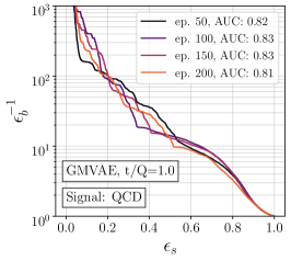
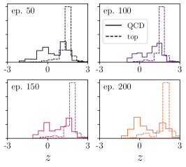
Figure 5: Results for the 1D GMVAE. In the large panels we show the ROC curves for tagging top and QCD as signal. In the small panels we show the distributions of the top and QCD jets in the latent space developed over the training.

Latent-space tagging

For this study of the GMVAE we use the exact same architecture as for the VAE except for the new latent space prior, see Fig. 4. We present the results for the classification of QCD and top jets in latent space in Fig. 5. It’s clear that the Gaussian mixture prior is shaping the latent space, and the network has the same benefit as the VAE in that the latent representation of the jets stabilises as the training converges. However we do not see an increase in performance in going from the VAE to the GMVAE. The reason for this is that while the top jets occupy just one mode in latent space, the QCD jets occupy both. Upon inspecting the jets which are assigned to each mode we find that this assignment is based on the amount of pixel activity within the jet, rather than on the specific features in the jet. We also experimented with using larger latent spaces, keeping the number of modes at two. This resulted in much better reconstruction accuracy and the bi-modal latent space structure persisted, however the performance of the latent space classification did not improve.

4 Dirichlet-VAE

Finally, we follow an alternative approach to provide the VAE with a geometry that leads to a mode separation. We do this by using the Dirichlet distribution, a family of continuous multivariate probability distributions, as the latent space prior. It has the following probability density function:

$$\mathcal{D}_{\alpha}(r)=\frac{\Gamma(\sum_{i}\alpha_{i})}{\prod_{i}\Gamma(\alpha_{i})}\;\prod_{i}r_{i}^{\alpha_{i}-1},\qquad\text{with}\;i=1~{}...~{}R\;.$$ (14)

This $R$-dimensional Dirichlet is parameterised by $R$ hyper-parameters $\alpha_{i}>0$, while the function itself is defined on an $R$-dimensional simplex. The Dirichlet distribution is conjugate to the multinomial distribution and is commonly used in Bayesian statistics as a prior in multinomial mixture models. The expectation values for the sampled vector components are $\langle r_{i}\rangle=\alpha_{i}/\sum_{j}\alpha_{j}$, so as a prior it will create a hierarchy among different mixture components. In our application, it imposes a compact latent space, whose latent dimensions can be interpreted as mixture weights in a multinomial mixture model [49, 50].

Loss and network

For a Dirichlet structure in the latent space, the re-parametrization trick requires some attention. We opt to use a softmax Gaussian approximation to the Dirichlet distribution [49], because the re-parametrization of Gaussian sampling is straightforward and stable,

$$r\sim\text{softmax}\,\mathcal{N}(z;\tilde{\mu},\tilde{\sigma}) \approx\mathcal{D}_{\alpha}(r)$$

$$\text{with}\quad\tilde{\mu}_{i} =\log\alpha_{i}-\frac{1}{R}\sum_{i}\log\alpha_{i}$$

$$\tilde{\sigma}_{i} =\frac{1}{\alpha_{i}}\left(1-\frac{2}{R}\right)+\frac{1}{R^{2}}\sum_{i}\frac{1}{\alpha_{i}}\;.$$ (15)

With this approximation the encoder network $q_{\phi}(r|x)$ plays the same role as in the VAE and the GMVAE, with the encoder outputs corresponding to the means and variances of the Gaussians in the softmax approximation.

The loss function of the Dirichlet-VAE (DVAE) includes the usual reconstruction loss and latent loss. For the reconstruction loss we use the cross-entropy between the inputs and the outputs [49]. The latent loss is given by the KL-divergence between the per-jet latent space representation and the Dirichlet prior, with a pre-factor $\beta_{\text{KL}}$. It is easily calculated for the Gaussians in the softmax approximation of the Dirichlet distribution and the Gaussians defined by the encoder output [49],

$$\mathcal{L} =\Big{\langle}-\big{\langle}\log p_{\theta}(x|r)\big{\rangle}_{q_{\phi}(r|x)}+\beta_{\text{KL}}D_{\text{KL}}(q_{\phi}(r|x),\mathcal{D}_{\alpha}(r))\Big{\rangle}_{p_{\text{data}}(x)}\;,$$

$$D_{\text{KL}}(q_{\phi}(r|x),\mathcal{D}_{\alpha}(r))=\frac{1}{2}\sum_{i=1}^{R}\left(\frac{\tilde{\sigma}_{i}^{2}}{\sigma_{i}^{2}}+\frac{(\tilde{\mu}_{i}-\mu_{i})^{2}}{\sigma_{i}^{2}}-R-\log\frac{\sigma_{i}^{2}}{\tilde{\sigma}_{i}^{2}}\right).$$ (16)

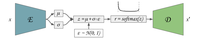
Figure 6: Architecture for the Dirichlet VAE. The approximate Dirichlet prior is indicated by the softmax step and the bi-modal distribution shown above it.

Unlike with the GMVAE, we do not make the parameters of the prior learnable. We employ a very simple DVAE architecture, shown in Fig. 6. The encoder is a fully connected network with 1600 inputs, corresponding to the $40\times 40$ image, and $2R$ outputs, where $R$ refers to the dimension of the Dirichlet latent space. We also insert a hidden layer of 100 nodes with SeLU activations and use linear activations on the output layer. The decoder is also a fully connected network with $R$ nodes in the input layer, 1600 nodes in the output layer and no hidden layers. We do not allow biases in the decoder, and apply a softmax activation to the output layer.

The Dirichlet latent space has the advantage that the sampled $r_{i}$ can be interpreted as mixture weights of mixture components describing the jets. If we view the DVAE as an inference tool for a multinomial mixture model, these mixture components correspond to probability distributions over the image pixels. These distributions enter into the likelihood function of the model, which is parameterised by the decoder network. In a simple example with two mixtures, $R=2$, the latent space is described by $r_{1}\in[0,1]$, with $r_{0}\!=\!1-r_{1}$ fixed. The pure component distributions are given by $p_{\theta}(x|r_{1}\!=\!0)$ and $p_{\theta}(x|r_{1}\!=\!1)$, and any output for $r_{1}\in[0,1]$ is a combination of these two distributions. Our simple decoder architecture exactly mimics this scenario. In the absence of hidden layers and biases the decoder network has exactly $R\times 1600$ parameters to describe the two mixture component distributions. One caveat is that we apply the softmax activation to the linear combination of outputs on the output layer, rather than to the outputs corresponding to each mixture separately. In Ref. [49] it is explained how this is related to the application of an ensemble technique called product of experts.

Latent-space tagging

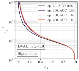
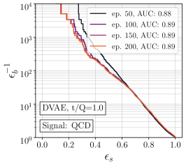
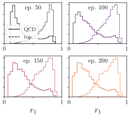
Figure 7: Results for the DVAE. In the large panels we show the ROC curves for tagging top and QCD as signal. In the small panels we show the distributions of the top and QCD jets in the latent space developed over the training.

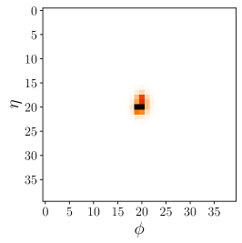
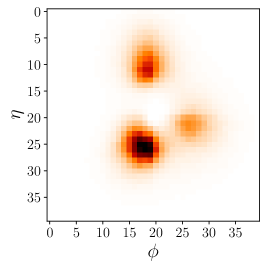
Figure 8: Visualisation of the decoder weights, interpreted as the mixture distributions for $p_{\theta}(x|r_{1}\!=\!0)$ (left) and $p_{\theta}(x|r_{1}\!=\!1)$ (right) learned by the DVAE decoder.

To compare with the AE and VAE studies in Fig. 3 and the GMVAE in Fig. 5 we start by training on 100k QCD and top jets each. We use a 2D Dirichlet latent space with $\alpha_{1,2}=1$, where due to the simplex nature of the Dirichlet only one latent space variable is independent. We choose $\beta_{\text{KL}}\!=\!0.1$ so that the prior has a large effect on the training. We compare QCD and top tagging and show the latent space distributions in Fig. 7. The visualisations of the decoder weights, i.e. the mixture component distributions $p_{\theta}(x|r_{0}=1)$ and $p_{\theta}(x|r_{0}=0)$, are shown in Fig. 8.

The advantages of the DVAE are immediately clear. First, the performance improves from an AUC of $0.83$ for the VAE to $0.89$ for the DVAE. Second, the latent space of the DVAE is a better and more stable description of the multi-class jet sample. It quickly settles into a clear bi-modal pattern with equal importance given to both modes. The QCD mode peaks at $r_{1}=0$, indicating that the $p_{\theta}(x|r_{1}\!=\!0)$ mixture describes QCD jets, while the top mode peaks at $r_{1}=1$, indicating that the $p_{\theta}(x|r_{1}\!=\!1)$ mixture describes top jets. This is confirmed by visualizing the decoder weights in Fig. 8. Comparing these to the truth-level jet images in Fig. 1 we see the clear correspondence between the learned mixture distributions and the actual images, so the DVAE has learned to separate the top-specific and QCD-specific features into the different mixtures.

Anomaly detection

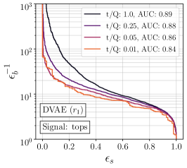
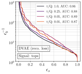
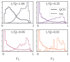
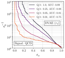
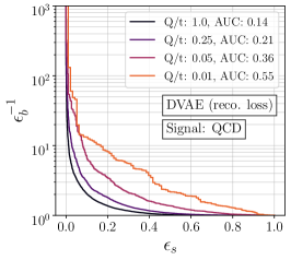
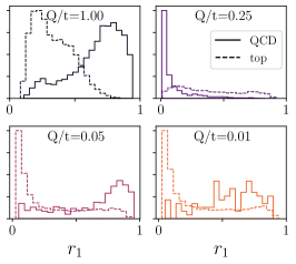
Figure 9: DVAE results for various amounts of anomalous top (upper) and QCD (lower) jets in the sample, where the mixture weights (left) and the reconstruction loss (middle) are used for classification. In the small panels we show the distributions of the top and QCD jets in the latent space.

Moving towards a more realistic scenario of unsupervised classification, we need to study scenarios with a class imbalance, where one of these classes is viewed as anomalous. We slightly adapt our hyper-parameters to more hierarchic sub-class proportions [12] and choose $\alpha_{1,2}=(1.0,0.25)$ when we have a class imbalance in the data. The performance of the network is not overly sensitive to the actual values. The benefit is that the DVAE will assign the dominant class of jets to $r_{1}\!=\!0$, so we should find that anomalous jets are pushed towards $r_{1}\!=\!1$.

We consider four different signal-to-background ratios, $1.00$, $0.25$, $0.05$, and $0.01$, where the latter two can be considered anomalous. In the top row of Fig. 9 we show results for the case where the signal is top jets, and in the bottom row for QCD jets. We plot the ROC curves using the latent space and using the reconstruction error, and then plot the latent space distributions for the different signal-to-background ratios.

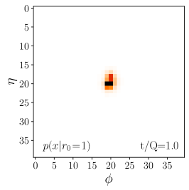
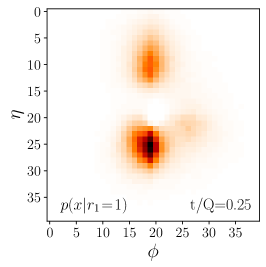
Figure 10: Learned mixture distributions extracted from the decoder weights with various amounts of anomalous top jets in the sample.

When the top jets are the signal, the classification based on mixture weights works best for $t/Q=1.0$ and degrades towards smaller ratios $t/Q$. This is expected since the latent space requires information about many jets of a class to accurately construct a good latent representation for it. In contrast, the performance of the reconstruction loss improves as we decrease $t/Q$, since the network will typically reconstruct an under-represented class poorly. This is why we find a reasonably good performance for anomalous top-tagging at $t/Q=0.01$, as reported in Ref. [1, 2, 66, 67]. The picture changes when the QCD jets are the signal. While the latent space tagging with appropriate latent spaces is stable, the reconstruction error fails as a classifier. This reflects the motivation of this study, discussed in Sec. 2, as well as the power of our new approach.

The latent space distributions in Fig. 9 confirm that when one class is anomalous, the Dirichlet prior helps in assigning the dominant class to the mixtures $r_{1}\!=\!0$. One outlier here is the case $Q/t\!=\!0.25$, where QCD jets are, accidentally, assigned to $r_{1}\!=\!0$. This can happen because also top jets have a strong central prong and copy the typical QCD jet feature. Because the unsupervised DVAE does not know the truth label and only assigns features to classes, the dominant feature even when $Q/t=0.25$ turns out QCD-like.

As before, we can use the visualisation of the decoder weights to study what the DVAE has learned. In Fig. 10 we show this visualisation for the top-tagging runs in Fig. 9. As $t/Q$ in the training data is decreased, the $p_{\theta}(x|r_{1}\!=\!1)$ mixture transforms from the 3-prong top-like structure to a 2-prong structure that is quite prevalent already in the QCD jet sample.

Enlarging the latent space

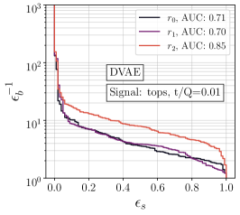
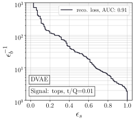
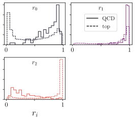
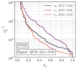
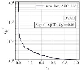
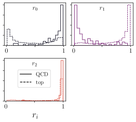
Figure 11: DVAE results using 3 mixture components ($R=3$) for various amounts of anomalous top (upper) and QCD (lower) jets in the sample, where the mixture weights (left) and the reconstruction loss (middle) are used for classification. In the small panels we show the distributions of QCD and tops along each direction in latent space.

Clearly, there will be applications where a 1D latent space or $R\!=\!2$ is not enough to construct a sufficient representation of the data for anomaly detection. With this in mind we enlarge the latent space to $R\!=\!3$ and again study the anomalous top ($t/Q\!=\!0.01$) and anomalous QCD ($Q/t\!=\!0.01$) scenarios. We choose a hierarchical prior through $\alpha_{i}=(1.0,0.25,0.1)$, such that the mixtures are ordered by their prevalence in the sample. This forces the network to focus on different scales in the data-set, instead of describing just the most common patterns in the data.

In Fig. 11 we show the DVAE results for $R\!=\!3$ using each of the latent mixture weights separately as the classifier. With anomalous top jets, the $r_{2}$-mixture weight corresponding to the weakest class always produces the best classifier. In contrast, for anomalous QCD jets, the best classifier is the $r_{1}$-mixture, with a larger weight than $r_{2}$ in the prior. Compared to the $R\!=\!2$ case, the performance in anomalous QCD tagging here is strikingly better, with an AUC of $0.91$. A closer look at Fig. 9 already indicates that the dominant, feature-rich top jets require both mixtures to describe their range of features. This is enhanced by the fact that there is a lot of variability within the top jet sample, and is to some degree dependent on the pre-processing.

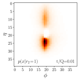
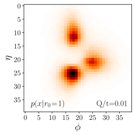
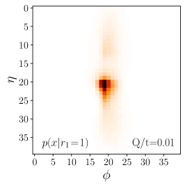
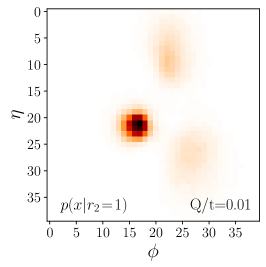
Figure 12: Three learned mixture distributions extracted from the decoder weights for $t/Q=0.01$ (upper) and $Q/t=0.01$ (lower). The mixtures are shown in order of their prevalence in the jet sample.

To understand the symmetric performance of the expanded DVAE, we look at the three learned mixture distributions for $t/Q=0.01$ and for $Q/t=0.01$ in Fig. 12. In the anomalous top case (top row) the sample is mostly QCD jets, as reflected in the mixture distributions. Because of the hierarchical prior, we see that the less prevalent the mixture component the wider the angular splitting in the mixture distribution gets. The top jets typically contain wide angle splittings, which explains why they are assigned larger weights in the $r_{2}$ mixture than in the others. Due to the jet pre-processing and the fact that QCD are jets are mostly one-prong or two-prong, the images are expected to be almost symmetric in the $\eta$ and $\phi$ plane. Interestingly, from the mixture distributions we can see that the DVAE has learned these approximate separate symmetries. Because we use fully-connected networks with pixelized input images and without any convolutions, the only information about the locality of the pixels or the symmetries must be learned from the jet images.

In the learned mixture distributions for the anomalous QCD case (bottom row), the sample is mostly top jets, and the large differences in the learned distributions highlights the amount of variance within the top jets alone. This is a strong indication that we do need more latent dimensions to describe the top jets. We also see that the $r_{1}$ mixture is very QCD-like, even though it is not the least prevalent mixture. This implies that QCD-like features are prevalent in the top jets. This is different from the anomalous top jets, where key top-features are missing in the QCD jet sample. This explains why QCD jets do not generate a large reconstruction error in a VAE trained on predominantly top jets. It also explains why the ROC curves for QCD-tagging have much lower mis-tagging rates at low signal efficiencies than the ROC curves for top-tagging.

The Gibbs triangles in Fig. 13 provide a useful visualisation of how the jets are distributed in the $R\!=\!3$ Dirichlet latent space. This visualisation is possible because the latent space is defined on a simplex with $\sum_{i}r_{i}=1$. Only two of the variables are free due to the constraint, but rather than just selecting two arbitrary directions we can use the constraint to project the three variables onto a 2D plane that captures all three directions equally. The points on the triangle represent the latent space coordinates $(1,0,0)$, $(0,1,0)$, and $(0,0,1)$, allowing us to see exactly where the jets are encoded. In the left panel we see the prior distribution and the hierarchy imposed on the three directions by the choice of hyper-parameters. On the top row we have the latent representations for the jets in the anomalous top jet (center) and anomalous QCD jet (right) cases, while in the second row we show examples of jets generated from these specific points in latent space. We see that the DVAE is learning a structured and hierarchic latent space mapping for the jets, allowing the rarer features within the data-set to occupy significant regions of latent space. Importantly, the anomalous jets in both, the anomalous top and the anomalous QCD cases, are isolated in latent space. Going back to the start of this paper, this is exactly what is not possible using the reconstruction error.

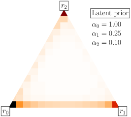
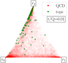
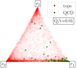
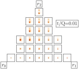
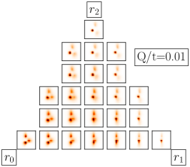
Figure 13: Gibbs triangle plots, also known as the Ternary plots or de Finetti diagrams, for the $R\!=\!3$ Dirichlet latent space. Top row: the prior distribution (left) on the latent space, and the distributions of jets for anomalous top (centre) and QCD (right). Bottom row: visualisations from the latent space of the models trained in the anomalous tops and anomalous QCD scenarios.

5 Outlook

In this paper we studied how different latent spaces in VAEs can facilitate improved unsupervised jet classification and can allow for the direct interpretation of what is being learned by the neural networks. We started with a brief review of the AE and VAE and discussed the drawbacks of both reconstruction error classification and latent space classification. In particular we discussed the problem of classifying anomalous jets which have less structure than the dominant class in the sample, with the prime example being tagging anomalous QCD jets in a sample of predominantly top jets.

The work is guided by the idea that autoencoders should make use of the latent space geometry to develop modes that represent classes of features in the data-set, and that background and signal should somehow separate into these modes. We started by studying the Gaussian-Mixture-VAE where we observe that the multi-modal latent space did indeed provide a multi-modal encoding of the jets. The issue was that the modes did not represent all relevant classes of features within the data-set. Then we studied the Dirichlet-VAE, which accurately determined hierarchic classes of features in the data-set, and organised the jets in a way which separates the signal and background. With a simple decoder architecture we were able to interpret the decoder weights as mixture distributions corresponding to each of the latent space directions. They could be visualised for a direct interpretation of what the network learns.

While the $R\!=\!2$ Dirichlet latent space worked well for top-tagging, the network still did not tag anomalous QCD jets in a sample of predominantly top jets symmetrically. In going to an $R\!=\!3$ latent space the network isolated the QCD-like features in latent space leading to a massive improvement in the classification. The larger latent space combined with a hierarchical prior provided a latent space capable of extracting features of varying prevalences in the data-set. With these structures, we have shown that problems of finding anomalous jets with less structure than the dominant class in the data-set can be solved through choosing better latent space structures. This opens the door to more effective jet anomaly detection methods for use in collider analyses.

Note added: the submission of this paper is coordinate with Ref. [68] and Ref. [69] on related approaches to the same problem with unsupervised learning and autoencoders.

Acknowledgments

This project was inspired by discussions and presentations during the Anomaly Detection Mini-Workshop — LHC Summer Olympics 2020 at Hamburg University [70, 71] and during the TRR 257 mini-workshop on Machine Learning. As always, we would like to thank Gregor Kasieczka for great discussion on all aspects of machine learning at the LHC. In addition, we are very grateful for many discussions with the Aachen and Rutgers groups, leading to a coordinated preprint submission. BMD would like to thank the Ljubljana group for early discussions on Dirichlet latent spaces, and the general application of VAEs in anomaly detection. The research of TP is supported by the Deutsche Forschungsgemeinschaft (DFG, German Research Foundation) under grant 396021762 – TRR 257 Particle Physics Phenomenology after the Higgs Discovery. CS is supported by the International Max Planck School Precision Tests of Fundamental Symmetries. PS is partly supported by the DFG Research Training Group GK-1940, Particle Physics Beyond the Standard Model. BMD is supported by funding from BMBF.

Appendix A Unsupervised Lund plane

Lund-plane images

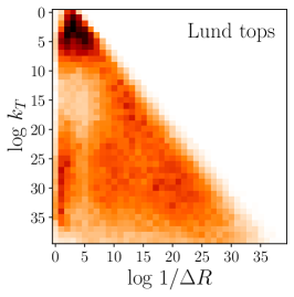
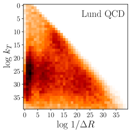
Figure 14: Average of 100k QCD and top jet images in the primary Lund plane representation. The $x$ and $y$ axis show the pixel numbers, but these axis go from $0$ to $6$ and $-2$ to $5$, respectively.

To analyse jets in the Lund plane [72, 73], we start by re-clustering them using the C/A algorithm. The algorithm finds the two constituents closest to each other in the $(\eta,\phi)$ plane and combines them to a single constituent or subjet. This $2\!\rightarrow\!1$ re-clustering continues until all constituents (and subjets) are clustered into one jet. The Lund plane representation follows from undoing this clustering piece by piece. At each step we split a subjet into two further subjets, $j_{a}\rightarrow j_{b}j_{c}$, where $j_{b,c}$ are referred to as the daughter subjets and $j_{a}$ as the parent subjet. From them we calculate the observables

$$\Delta R_{b,c} =\sqrt{(\eta_{b}-\eta_{c})^{2}+(\phi_{b}-\phi_{c})^{2}}\qquad\qquad k_{T} =p_{T,b}\Delta R_{b,c}\quad\text{where}\;p_{T,b}>p_{T,c}$$

$$m_{a}^{2} =p_{a}^{2}=(p_{b}+p_{c})^{2} d =\text{max}(m_{b}/m_{a},m_{c}/m_{a})$$

$$z =p_{T,b}/(p_{T,b}+p_{T,c}) \kappa =z\Delta R_{b,c}.$$ (17)

We then assign each splitting to a primary, secondary, etc Lund plane using the simple algorithm

1. uncluster $j_{a}\rightarrow j_{b}j_{c}$

2. assign $l\!=\!0(1)$ to the daughter with the larger (smaller) $p_{T}$

3. perform the next step in the unclustering, e.g. $j_{c}\rightarrow j_{d},j_{e}$

4. assign $l\!=\!0(1)$ to the daughter with the larger (smaller) $p_{T}$

5. add the $l$ from the parent $j_{c}$ to the $l$’s assigned to the daughters $j_{d}$ and $j_{e}$

6. repeat steps 3-5 until the jet is completely unclustered.

At the end, each splitting comes with a set of observables and an $l$-value. We identify $l=0$ as the primary Lund plane, $l=1$ as the secondary Lund plane, and so on. This way the primary Lund plane contains all splittings from the hardest $p_{T}$-core of the jet, while the secondary Lund plane contains splittings once removed from this hardest $p_{T}$-core, and so on.

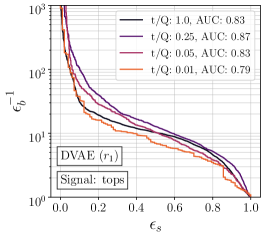
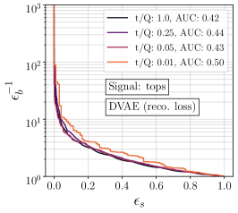
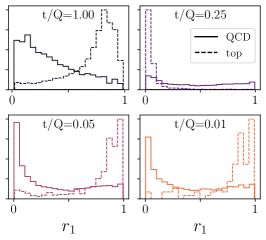
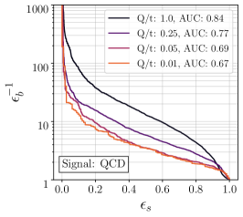
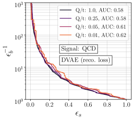
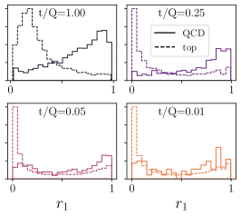
Figure 15: DVAE results using the Lund plane for various amounts of top (upper) and QCD (lower) jets in the sample, where the mixture weights (left) and the reconstruction loss (middle) of each jet are used for classification. In the small panels we show the distributions of the top and QCD jets in the latent space.

For our DVAE analysis we only use only the observables $\log k_{T}\in[-2,5]$ and $\log 1/\Delta R\in[0,6]$ and represent the Lund plane as $40\times 40$ images, just as before. In Fig. 14 we plot the average of 100k jet images for top and QCD, in the primary Lund plane. Because the main differences between the QCD and top jets should appear in the primary Lund plane, we will only use it for now. The DVAE training and architecture used here is identical to what we used for the jet images (Fig. 6).

In Fig. 15 we show results in scenarios with varying numbers of top jets and varying numbers of QCD jets. The unique aspect of the Lund plane results in comparison to the jet images is that the reconstruction error does not work here for tagging anomalous QCD jets or anomalous top jets. It seems that this is due to the truth level distributions for the QCD and top jets in the Lund plane representation having a very large overlap, differing only in the large angle and large $k_{T}$ region. Despite this, the DVAE still separates the two jet classes in the latent space. In viewing these results we note that there may be several routes to improving them; (i) weight the pixels by $k_{T}$ or another Lund observable, (ii) cut off non-perturbative regions of the Lund plane during the pre-processing. We did perform some tests with the pixel weights but the results did not show an improvement, alternatives were not fully explored in this analysis.

References

- [1] T. Heimel, G. Kasieczka, T. Plehn, and J. M. Thompson, QCD or What?, SciPost Phys. 6 (2019) 3, 030, arXiv:1808.08979 [hep-ph].
- [2] M. Farina, Y. Nakai, and D. Shih, Searching for New Physics with Deep Autoencoders, Phys. Rev. D 101 (2020) 7, 075021, arXiv:1808.08992 [hep-ph].
- [3] T. S. Roy and A. H. Vijay, A robust anomaly finder based on autoencoder, arXiv:1903.02032 [hep-ph].
- [4] A. Blance, M. Spannowsky, and P. Waite, Adversarially-trained autoencoders for robust unsupervised new physics searches, JHEP 10 (2019) 047, arXiv:1905.10384 [hep-ph].
- [5] D. P. Kingma and M. Welling, Auto-encoding variational bayes, arXiv:1312.6114 [stat.ML].
- [6] O. Cerri, T. Q. Nguyen, M. Pierini, M. Spiropulu, and J.-R. Vlimant, Variational Autoencoders for New Physics Mining at the Large Hadron Collider, JHEP 05 (2019) 036, arXiv:1811.10276 [hep-ex].
- [7] T. Cheng, J.-F. Arguin, J. Leissner-Martin, J. Pilette, and T. Golling, Variational Autoencoders for Anomalous Jet Tagging, arXiv:2007.01850 [hep-ph].
- [8] B. Bortolato, B. M. Dillon, J. F. Kamenik, and A. Smolkovič, Bump Hunting in Latent Space, arXiv:2103.06595 [hep-ph].
- [9] J. H. Collins, K. Howe, and B. Nachman, Anomaly Detection for Resonant New Physics with Machine Learning, Phys. Rev. Lett. 121 (2018) 24, 241803, arXiv:1805.02664 [hep-ph].
- [10] J. H. Collins, K. Howe, and B. Nachman, Extending the search for new resonances with machine learning, Phys. Rev. D99 (2019) 1, 014038, arXiv:1902.02634 [hep-ph].
- [11] B. M. Dillon, D. A. Faroughy, and J. F. Kamenik, Uncovering latent jet substructure, Phys. Rev. D100 (2019) 5, 056002, arXiv:1904.04200 [hep-ph].
- [12] B. M. Dillon, D. A. Faroughy, J. F. Kamenik, and M. Szewc, Learning the latent structure of collider events, Journal of High Energy Physics 2020 (Oct, 2020) .
- [13] A. Andreassen, B. Nachman, and D. Shih, Simulation Assisted Likelihood-free Anomaly Detection, Phys. Rev. D 101 (2020) 9, 095004, arXiv:2001.05001 [hep-ph].
- [14] C. K. Khosa and V. Sanz, Anomaly Awareness, arXiv:2007.14462 [cs.LG].
- [15] O. Knapp, G. Dissertori, O. Cerri, T. Q. Nguyen, J.-R. Vlimant, and M. Pierini, Adversarially Learned Anomaly Detection on CMS Open Data: re-discovering the top quark, arXiv:2005.01598 [hep-ex].
- [16] B. Nachman and D. Shih, Anomaly Detection with Density Estimation, Phys. Rev. D 101 (2020) 075042, arXiv:2001.04990 [hep-ph].
- [17] J. A. Aguilar-Saavedra, J. H. Collins, and R. K. Mishra, A generic anti-QCD jet tagger, JHEP 11 (2017) 163, arXiv:1709.01087 [hep-ph].
- [18] V. Mikuni and F. Canelli, UCluster: Unsupervised clustering for collider physics, arXiv:2010.07106 [physics.data-an].
- [19] K. Benkendorfer, L. L. Pottier, and B. Nachman, Simulation-Assisted Decorrelation for Resonant Anomaly Detection, arXiv:2009.02205 [hep-ph].
- [20] J. Hajer, Y.-Y. Li, T. Liu, and H. Wang, Novelty Detection Meets Collider Physics, arXiv:1807.10261 [hep-ph].
- [21] O. Amram and C. M. Suarez, Tag N’ Train: a technique to train improved classifiers on unlabeled data, JHEP 01 (2021) 153, arXiv:2002.12376 [hep-ph].
- [22] ATLAS, G. Aad et al., Dijet resonance search with weak supervision using TeV collisions in the ATLAS detector, Phys. Rev. Lett. 125 (2020) 13, 131801, arXiv:2005.02983 [hep-ex].
- [23] G. Kasieczka et al., The LHC Olympics 2020: A Community Challenge for Anomaly Detection in High Energy Physics, arXiv:2101.08320 [hep-ph].
- [24] R. T. D’Agnolo and A. Wulzer, Learning New Physics from a Machine, Phys. Rev. D99 (2019) 1, 015014, arXiv:1806.02350 [hep-ph].
- [25] R. T. D’Agnolo, G. Grosso, M. Pierini, A. Wulzer, and M. Zanetti, Learning multivariate new physics, Eur. Phys. J. C 81 (2021) 1, 89, arXiv:1912.12155 [hep-ph].
- [26] A. De Simone and T. Jacques, Guiding New Physics Searches with Unsupervised Learning, Eur. Phys. J. C79 (2019) 4, 289, arXiv:1807.06038 [hep-ph].
- [27] A. Mullin, S. Nicholls, H. Pacey, M. Parker, M. White, and S. Williams, Does SUSY have friends? A new approach for LHC event analysis, JHEP 02 (2021) 160, arXiv:1912.10625 [hep-ph].
- [28] M. Romão Crispim, N. Castro, R. Pedro, and T. Vale, Transferability of Deep Learning Models in Searches for New Physics at Colliders, Phys. Rev. D 101 (2020) 3, 035042, arXiv:1912.04220 [hep-ph].
- [29] M. C. Romao, N. Castro, J. Milhano, R. Pedro, and T. Vale, Use of a Generalized Energy Mover’s Distance in the Search for Rare Phenomena at Colliders, arXiv:2004.09360 [hep-ph].
- [30] B. Nachman, Anomaly Detection for Physics Analysis and Less than Supervised Learning, arXiv:2010.14554 [hep-ph].
- [31] P. Thaprasop, K. Zhou, J. Steinheimer, and C. Herold, Unsupervised Outlier Detection in Heavy-Ion Collisions, arXiv:2007.15830 [hep-ex].
- [32] P. T. Komiske, E. M. Metodiev, and J. Thaler, The Hidden Geometry of Particle Collisions, JHEP 07 (2020) 006, arXiv:2004.04159 [hep-ph].
- [33] P. T. Komiske, R. Mastandrea, E. M. Metodiev, P. Naik, and J. Thaler, Exploring the Space of Jets with CMS Open Data, Phys. Rev. D 101 (2020) 3, 034009, arXiv:1908.08542 [hep-ph].
- [34] P. T. Komiske, E. M. Metodiev, and J. Thaler, Metric Space of Collider Events, Phys. Rev. Lett. 123 (2019) 4, 041801, arXiv:1902.02346 [hep-ph].
- [35] O. Knapp, O. Cerri, G. Dissertori, T. Q. Nguyen, M. Pierini, and J.-R. Vlimant, Adversarially Learned Anomaly Detection on CMS Open Data: re-discovering the top quark, Eur. Phys. J. Plus 136 (2021) 2, 236, arXiv:2005.01598 [hep-ex].
- [36] K. T. Matchev, P. Shyamsundar, and J. Smolinsky, A quantum algorithm for model independent searches for new physics, arXiv:2003.02181 [hep-ph].
- [37] M. Crispim Romão, N. F. Castro, and R. Pedro, Finding New Physics without learning about it: Anomaly Detection as a tool for Searches at Colliders, Eur. Phys. J. C 81 (2021) 1, 27, arXiv:2006.05432 [hep-ph].
- [38] J. A. Aguilar-Saavedra, F. R. Joaquim, and J. F. Seabra, Mass Unspecific Supervised Tagging (MUST) for boosted jets, JHEP 03 (2021) 012, arXiv:2008.12792 [hep-ph].
- [39] M. van Beekveld, S. Caron, L. Hendriks, P. Jackson, A. Leinweber, S. Otten, R. Patrick, R. Ruiz de Austri, M. Santoni, and M. White, Combining outlier analysis algorithms to identify new physics at the LHC, arXiv:2010.07940 [hep-ph].
- [40] S. E. Park, D. Rankin, S.-M. Udrescu, M. Yunus, and P. Harris, Quasi Anomalous Knowledge: Searching for new physics with embedded knowledge, arXiv:2011.03550 [hep-ph].
- [41] J. H. Collins, P. Martín-Ramiro, B. Nachman, and D. Shih, Comparing Weak- and Unsupervised Methods for Resonant Anomaly Detection, arXiv:2104.02092 [hep-ph].
- [42] J. Tomczak and M. Welling, VAE with a VampPrior, in International Conference on Artificial Intelligence and Statistics, PMLR. 2018. arXiv:1705.07120 [cs.LG].
- [43] N. Dilokthanakul, P. A. Mediano, M. Garnelo, M. C. Lee, H. Salimbeni, K. Arulkumaran, and M. Shanahan, Deep unsupervised clustering with Gaussian mixture variational autoencoders, arXiv preprint arXiv:1611.02648 (2016) , arXiv:1611.02648 [cs.LG].
- [44] J. Shao and X. Li, Generalized zero-shot learning with multi-channel Gaussian mixture VAE, IEEE Signal Processing Letters 27 (2020) 456.
- [45] L. Yang, N.-M. Cheung, J. Li, and J. Fang, Deep clustering by Gaussian mixture variational autoencoders with graph embedding, in Proceedings of the IEEE/CVF International Conference on Computer Vision. 2019.
- [46] Y. Guo, W. Liao, Q. Wang, L. Yu, T. Ji, and P. Li, Multidimensional time series anomaly detection: A GRU-based Gaussian mixture variational autoencoder approach, in Asian Conference on Machine Learning, PMLR. 2018.
- [47] R. Shu, J. Brofos, F. Zhang, H. H. Bui, M. Ghavamzadeh, and M. Kochenderfer, Stochastic video prediction with conditional density estimation, in ECCV Workshop on Action and Anticipation for Visual Learning. 2016.
- [48] J. R. Hershey and P. A. Olsen, Approximating the Kullback Leibler divergence between Gaussian mixture models, in 2007 IEEE International Conference on Acoustics, Speech and Signal Processing-ICASSP’07, IEEE. 2007.
- [49] A. Srivastava and C. Sutton, Autoencoding variational inference for topic models, arXiv:1703.01488 [stat.ML].
- [50] W. Joo, W. Lee, S. Park, and I.-C. Moon, Dirichlet variational autoencoder, arXiv:1901.02739 [cs.LG].
- [51] E. M. Metodiev and J. Thaler, Jet Topics: Disentangling Quarks and Gluons at Colliders, Phys. Rev. Lett. 120 (2018) 24, 241602, arXiv:1802.00008 [hep-ph].
- [52] P. T. Komiske, E. M. Metodiev, and J. Thaler, An operational definition of quark and gluon jets, JHEP 11 (2018) 059, arXiv:1809.01140 [hep-ph].
- [53] E. Alvarez, F. Lamagna, and M. Szewc, Topic Model for four-top at the LHC, JHEP 01 (2020) 049, arXiv:1911.09699 [hep-ph].
- [54] A. Butter et al., The Machine Learning Landscape of Top Taggers, SciPost Phys. 7 (2019) 014, arXiv:1902.09914 [hep-ph].
- [55] T. Sjöstrand, S. Ask, J. R. Christiansen, R. Corke, N. Desai, P. Ilten, S. Mrenna, S. Prestel, C. O. Rasmussen, and P. Z. Skands, An introduction to PYTHIA 8.2, Comput. Phys. Commun. 191 (2015) 159, arXiv:1410.3012 [hep-ph].
- [56] DELPHES 3, J. de Favereau, C. Delaere, P. Demin, A. Giammanco, V. Lemaître, A. Mertens, and M. Selvaggi, DELPHES 3, A modular framework for fast simulation of a generic collider experiment, JHEP 02 (2014) 057, arXiv:1307.6346 [hep-ex].
- [57] M. Cacciari, G. P. Salam, and G. Soyez, The anti- jet clustering algorithm, JHEP 04 (2008) 063, arXiv:0802.1189 [hep-ph].
- [58] M. Cacciari and G. P. Salam, Dispelling the myth for the jet-finder, Phys. Lett. B 641 (2006) 57, arXiv:hep-ph/0512210.
- [59] M. Cacciari, G. P. Salam, and G. Soyez, FastJet User Manual, Eur. Phys. J. C 72 (2012) 1896, arXiv:1111.6097 [hep-ph].
- [60] S. Macaluso and D. Shih, Pulling Out All the Tops with Computer Vision and Deep Learning, JHEP 10 (2018) 121, arXiv:1803.00107 [hep-ph].
- [61] M. Abadi, P. Barham, J. Chen, Z. Chen, A. Davis, J. Dean, M. Devin, S. Ghemawat, G. Irving, M. Isard, et al., Tensorflow: A system for large-scale machine learning, in 12th USENIX Symposium on Operating Systems Design and Implementation (OSDI 16). 2016.
- [62] F. Chollet et al., Keras, .
- [63] D. P. Kingma and J. Ba, Adam: A Method for Stochastic Optimization, arXiv:1412.6980 [cs.LG].
- [64] J. Batson, C. G. Haaf, Y. Kahn, and D. A. Roberts, Topological obstructions to autoencoding, arXiv:2102.08380 [hep-ph].
- [65] K. A. Ashman, C. M. Bird, and S. E. Zepf, Detecting bimodality in astronomical datasets, The Astronomical Journal 108 (Dec, 1994) 2348.
- [66] I. Oleksiyuk, Unsupervised learning for tagging anomalous jets at the LHC, Bachelor thesis, RWTH Aachen, 2020.
- [67] T. Finke, Deep Learning for New Physics Searches at the LHC, Master thesis, RWTH Aachen, 2020.
- [68] T. Finke, M. Kramer, A. Morandini, A. Muck, and I. Oleksiyuk, Autoencoders for unsupervised anomaly detection in high-energy physics, . (to appear).
- [69] Y. Gershtein, D. Jaroslawski, K. Nash, D. Shih, and M. Tran, Anomaly detection with convolutional autoencoders and latent space analysis, . (to appear).
- [70] B. M. Dillon, Learning the latent structure of collider events, . Anomaly Detection Mini-Workshop – LHC Summer Olympics 2020.
- [71] D. Jaroslawski and K. Nasha, Anomaly detection with convolutional autoencoders and latent space analysis, . Anomaly Detection Mini-Workshop – LHC Summer Olympics 2020.
- [72] F. A. Dreyer, G. P. Salam, and G. Soyez, The Lund Jet Plane, JHEP 12 (2018) 064, arXiv:1807.04758 [hep-ph].
- [73] S. Carrazza and F. A. Dreyer, Lund jet images from generative and cycle-consistent adversarial networks, Eur. Phys. J. C79 (2019) 11, 979, arXiv:1909.01359 [hep-ph].