B-modes from Post-inflationary Gravitational Waves Sourced by Axionic Instabilities at Cosmic Reionization

Abstract

We show that axion-like particles that only couple to invisible dark photons can generate visible B-mode signals around the reionization epoch. The axion field starts rolling shortly before reionization, resulting in a tachyonic instability for the dark photons. This generates an exponential growth of the dark photon quanta sourcing both scalar metric modes and gravitational waves that leave an imprint on the reionized baryons. The tensor modes modify the cosmic microwave background (CMB) polarization at reionization, generating visible B-mode signatures for the next generation of CMB experiments for parameter ranges that satisfy the current experimental constraints.

I Introduction

The discovery of gravitational waves (GW) at LIGO Aasi et al. (2015) and VIRGO Acernese et al. (2014) has motivated the search for other possible GW sources beyond the mergers of astrophysical objects. Among those, GWs from cosmological sources, such as strong first order phase transitions Caprini et al. (2020) and the presence of cosmic strings Auclair et al. (2020), are of particular interest in elucidating the early history of the universe (e.g., Geller et al. (2018); Cui et al. (2018)). The cosmological GW signals can have a wide range of possible frequencies: interferometer experiments can detect GWs with frequencies above $\sim 10^{-5}~{}$Hz Kawamura et al. (2011); Amaro-Seoane et al. (2017); Punturo et al. (2010); Crowder and Cornish (2005), and lower frequency signals down to $\sim 10^{-8}~{}$Hz are relevant for pulsar timing experiments Dewdney et al. (2009); Manchester (2013); if GWs have frequencies lower than $\sim 10^{-15}~{}$Hz, we can search for the B-mode polarization signals from GW imprints on the cosmic microwave background (CMB) Ade et al. (2015a). Such low-frequency signals have wavelengths comparable to the visible universe’s size and must have a cosmological origin. As a result, the B-mode signal is mainly considered to come from GWs produced during cosmic inflation (see Kamionkowski and Kovetz (2016) and the references therein).

In this letter, we propose a new source for B-mode generating GWs produced by axion-like particles (ALPs) around the time of cosmic reionization. Axions were originally proposed to solve the strong CP problem Peccei and Quinn (1977a, b) and realized to be a viable dark matter (DM) candidate Abbott and Sikivie (1983); Preskill et al. (1983); Dine and Fischler (1983); Co et al. (2018). ALPs generalize the cosmological phenomenology of axions without a necessary connection to strong CP. For example, an ALP can serve as the inflaton field responsible for the period of cosmic inflation Freese et al. (1990); Dimopoulos et al. (2008); Anber and Sorbo (2010) or as the relaxion, addressing the hierarchy problems in nature by varying the fundamental constants of nature with time  Hook and Marques-Tavares (2016); Fonseca et al. (2020); Graham et al. (2015). On the experimental side, several new direct detection experiments have been put into action Anastassopoulos et al. (2017); Du et al. (2018); Ouellet et al. (2019); Zhong et al. (2018) or have been proposed Liu et al. (2019); Bogorad et al. (2019); Hook et al. (2018); Caputo et al. (2019) to look for ALPs. Part of the theoretically-favored axion parameter space has already been experimentally excluded.

In the particular case where ALPs couple to dark photons, the ALP field’s rolling leads to a “tachyonic instability” that amplifies vacuum fluctuations of one of the dark photon helicities. The process generates exponential dark photon production, and similar phenomena have been studied under the context of inflation Anber and Sorbo (2010, 2012), production of dark photon DM Co et al. (2019), depletion of axion DM to avoid overclosure Agrawal et al. (2018), and friction for the relaxion models Hook and Marques-Tavares (2016); Fonseca et al. (2020). Recently it has been shown that the stochastic GW background generated through this process in the early universe may be detectable in interferometers or pulsar timing arrays Machado et al. (2019a, b). In Weiner et al. (2021), a similar mechanism at the recombination period is studied within the context of early dark energy solutions to the Hubble tension Bernal et al. (2016); Poulin et al. (2019) and is shown to produce visible GW signals in the CMB.

In this work, we consider a similar effect of producing a GW background from tachyonic particle production late in the universe’s history – after recombination and around the time of galaxy formation. As a tensor perturbation of the metric, the GW background leaves an imprint on the photon energy distribution. When the universe enters the reionization era at $z_{\rm rei}\approx 8$, CMB photons propagating in the line-of-sight direction get polarized by the last Thomson scattering, and a combination of the tensor perturbation and the angular distribution of the photon polarization produces the B-mode signal in the large-scale CMB spectrum. In particular, we will show that for parameter ranges of our model not currently excluded by existing or past experiments Aghanim et al. (2019); Ade et al. (2015b), we predict a B-mode signal accesible to the next generation of B-mode detectors.

The B-mode signals sourced by the axionic instability have a power spectrum which could be distinguished from those produced by inflationary GWs. An observation of such unique B-mode signals will be a discovery of dark sector physics and will shed light on the nature of dark energy by revealing that dark energy is changing at late times. In particular, a revelation that dark energy has recently changed by an amount close to its current value is suggestive of some dynamics related to the cosmological constant (CC) problem. As we will show, next-generation experiments will be able to probe such shifts on a scale similar to the current value of the cosmological constant.

We remark that our calculation utilizes a linear semi-classical approximation and therefore our results need to be confirmed by a full lattice study. We expect this to affect the precise predictions of the spectral shapes, but not our ultimate conclusions.

This paper is organised as follows: After reviewing the mechanism of tachyonic production of dark photons, we describe our setting and set up the calculation of dark photon’s energy density fluctuations in Sec. II. We then discuss the metric perturbation sourced by the dark photon fluctuation in Sec. III and show the derivation of the resulting CMB spectra. Subsequently, we present our results, comparing the predicted signals within two benchmark ALP models to the sensitivity of the future B-mode experiments and to the current constraints from Planck in Sec. IV. Finally, we conclude in Sec. V.

II The Model

II.1 Tachyonic production of dark photons

We consider an axion field $\phi$ coupled to a $U(1)$ dark photon, with the Lagrangian given by

$$\mathcal{L}=-\dfrac{1}{2}\partial_{\mu}\phi\partial^{\mu}\phi-V(\phi)-\dfrac{1}{4}F_{\mu\nu}F^{\mu\nu}-\dfrac{\alpha}{4f}\phi F_{\mu\nu}\tilde{F}^{\mu\nu}\,,$$ (1)

where $V(\phi)=\frac{1}{2}m^{2}\phi^{2}$, and $f$ is the axion constant. We assume the dark photon is massless and is produced only after inflation. The quadratic potential $V(\phi)$ can naturally arise from an axion-like potential $\Lambda^{4}\cos(\phi/f)$, which implies $m\sim\Lambda^{2}/f$. We consider $m$ close to the Hubble scale right before the reionization. We will see that in our setting, the CMB probes $\Lambda\sim{\cal O}({\rm meV})$, which also coincides with the order of magnitude of the cosmological constant, so that an observation of the signal we discuss may lead to new insights into dark energy .

The equation of motion of the axion field is then

$$\phi^{\prime\prime}+2aH\phi^{\prime}+a^{2}\frac{\partial V}{\partial\phi}=\frac{\alpha}{f}a^{2}{\bf E}\cdot{\bf B}\,,$$ (2)

in which $a$ is the scale factor of the FRW metric $ds^{2}=a^{2}(\tau)(d\tau^{2}-\delta_{ij}dx^{i}dx^{j})$, and $H$ is the Hubble parameter. The prime symbol denotes derivatives with respect to the conformal time $\tau$. On the right hand side of the equation, the dark electromagentic field serves as friction for the rolling of the axion $\phi$.

The rolling of the axion will cause the dark photon modes within a certain momentum range to grow exponentially, a phenomenon known as the tachyonic instability. This can be shown by examining the equation of motion of the dark photon field, which in the Coulomb gauge is written as

$$X_{i}=\int\mathcal{D}k\left(\epsilon_{+i}({\bf k})v_{+}(\tau,k)\hat{{\bf a}}_{+}({\bf k})e^{i{\bf k}\cdot{\bf x}}+h.c.\right),$$ (3)

$$X_{0}=0\,,$$

where $\mathcal{D}k\equiv d^{3}k/(2\pi)^{3}$. The creation and annihilation operators obey the commutation relation $[{\bf a}_{+}({\bf k}),\,{\bf a}^{\dagger}_{+}({\bf k^{\prime}})]=(2\pi)^{3}\delta({\bf k}-{\bf k}^{\prime})$, and the polarization vectors obey ${\bf k}\cdot{\bf\epsilon}_{\pm}=0$, ${\bf k}\times{\bf\epsilon}_{\pm}=\mp ik{\bf\epsilon}_{\pm}$, ${\bf\epsilon}_{\pm}\cdot{\bf\epsilon}_{\pm}=0$, ${\bf\epsilon}_{\pm}\cdot{\bf\epsilon}_{\mp}=1$. The dark photon field equation can then be written in terms of the mode function $v$ as

$$v^{\prime\prime}_{\pm}(k,\tau)+\omega^{2}_{\pm}(k,\tau)v_{\pm}(k,\tau)=0,$$ (4)

with the dispersion relation $\omega^{2}_{\pm}(k,\tau)=k^{2}\mp k\alpha\phi^{\prime}/f$. As long as the axion starts rolling and develops a non-zero $\phi^{\prime}$, the dark photon modes of a certain helicity in the momentum band $0<k<\alpha\lvert\phi^{\prime}\rvert/f$ will have $\omega^{2}(k,\tau)<0$ and therefore grow exponentially. Specifically, the $v_{+}$ modes can grow when $\phi^{\prime}>0$ and the $v_{-}$ modes grow when $\phi^{\prime}<0$, and the growth of the two helicities are alternating as the axion field oscillates around the minimum of its potential. The helicity experiencing the tachyonic instability right after axion starts the rolling will be significantly more enhanced than the other, as it spends more time in the tachyonic band.

To solve the axion and the dark photon coupled equations of motion, we treat the dark photon mode functions $v_{\pm}(k,\tau)$ as discretized modes of fixed $k$. And to the leading order, the reaction from dark photon field ${\bf E}\cdot{\bf B}$ on the right hand side of Eq. (2) is replaced by the expectation value $\langle{\bf E}\cdot{\bf B}\rangle$, which is calculated as

$$\langle{\bf E}\cdot{\bf B}\rangle=-\sum_{\lambda=\pm}\lambda\int\dfrac{k^{2}dk}{2\pi^{2}a^{4}}\,{\rm Re}\left[v^{\ast}_{\lambda}(k,\tau)v^{\prime}_{\lambda}(k,\tau)\right]\,.$$ (5)

II.2 Calculation setup

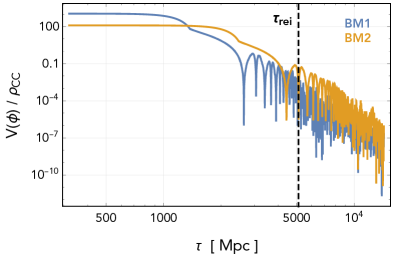
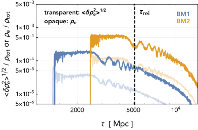
Figure 1: Left panel: The evolution of the axion potential energy of the two benchmark models we use, normalized by the dark energy density today $\rho_{CC}\approx 37~{}{\rm meV}^{4}$. Right panel: The evolution of the dark sector energy density $\rho_{e}$ and its perturbation $\langle\delta\rho^{2}_{e}\rangle^{1/2}$ induced by the tachyonic particle production, normalized by the total energy density of the universe, where $\langle\delta\rho^{2}_{e}\rangle^{1/2}\equiv\left[\int\mathcal{D}k\mathcal{D}k^{\prime}\langle\delta\rho_{e}(k)\delta\rho_{e}(k^{\prime})\rangle\right]^{1/2}$.

In our calculation, we assume the dark photon to be non-thermal such that its abundance comes only from the tachyonic production described above. We use 200 dark photon k-modes equally spaced on a logarithmic grid in the momentum range $[k_{\rm min},k_{\rm max}]$. The value of $k_{\rm max}$ is chosen such that $k_{\rm max}\gtrsim\alpha\lvert\phi^{\prime}\rvert_{\rm max}/f$, and we perform a consistency check with several choices of $k_{\rm max}$ to determine the number used for each calculation. The minimum value of the momentum range is set to be $k_{\rm min}=H_{0}/4$. With these choices, we make sure that the entirety of the momentum range of interest is covered.

In this work we do not include the back reaction of the gauge modes on the axion perturbations that requires a full lattice study (see Ratzinger et al. (2020)). This is mainly important for the axion abundance calculation which is not of interest in this setup. For the GWs, we expect the lattice results to be roughly consistent in magnitude Ratzinger et al. (2020) and to be mainly important for the spectral shape (see also Kitajima et al. (2018); Agrawal et al. (2020); Kitajima et al. (2020)). We therefore treat the calculation here as a preliminary estimate to motivate a full lattice study which is left for a subsequent work.

The produced dark photon k-modes are assumed to be in the Bunch-Davis vacuum $v_{\pm}(k,\tau)=e^{ik\tau}/\sqrt{2k}$ before the axion rolling starts and the axion field is released at an initial misalignment of $\lvert\phi_{0}\rvert=f$. We choose two benchmark models for which the tachyonic instability becomes significant after recombination but before reionization, taken as $z_{\rm rei}=8$. Note that keeping the axion mass fixed and varying the height of the initial misalignment (i.e. $\Lambda$ in our parameterization, keeping $f\propto\Lambda^{2}$) will only rescale the energy in the dark sector, and with it the energy density in the perturbations. Therefore we will think of the two benchmarks as two classes of models where the total energy in the dark sector remains a free parameter which can be constrained by current experimental data. We give the benchmark values of the parameters in Table 1, where we also show bounds on the energy scale in the dark sector $\Lambda_{\rm bound}$ which we derive in the following sections based on the uncertainty of the current power spectra measurements.

We plot the time evolution of the axion potential and the resulting inhomogeneities in the gauge modes in Fig. 1, using the two benchmark mark models and energy scale $\Lambda_{\rm bound}$. We see that the axions start their rolling shortly before the reionization and begin to oscillate around the minimum, producing the gauge mode inhomogeneity in the process. In Fig. 1 (right), we see that the dark photon energy is always below ${\cal O}(5\times 10^{-4})$ of the total energy. The process therefore gives negligible corrections to the angular diameter distance that relates to the CMB spectra. However, even though the average $\rho_{e}$ is small comparing to $\rho_{\rm tot}$ that is dominated by the matter density $\rho_{m}$, the density contrast of the dark photon energy is of $\mathcal{O}(1)$ as can be seen in the transparent and opaque curves. The energy perturbation $\langle\delta\rho_{e}^{2}\rangle^{1/2}$ is thus comparable to the matter density perturbation ($\sim 10^{-5}\rho_{m}$) that enters the horizon around the same time and can therefore generate visible signals as we show below.

	$m$ (eV)	$k_{\rm max}$ (Mpc-1)	$\Lambda_{\rm bound}$	$\alpha$
BM1	$4\times 10^{-30}$	0.94	16 meV	400
BM2	$8.8\times 10^{-31}$	0.78	9 meV	400

Table 1: The benchmark parameters used in the calculation.

III CMB spectra calculation

Although the axion starts rolling only after recombination, remarkably it can still modify the CMB perturbation observed today. The dark photon field enhanced by the tachyonic instability generates isocurvature perturbations that also source GWs Machado et al. (2019a) affecting the CMB power spectrum through the late integrated Sachs-Wolfe (ISW) effect. The produced GWs also leave an imprint in the CMB B-mode which will serve as our target signal for the discovery of this setup. Here we present the calculation of CMB $TT$, $EE$ and $BB$ spectra, $C_{\ell}^{TT}$, $C_{\ell}^{EE}$ and $C_{\ell}^{BB}$.

III.1 Scalar mode contribution

Perturbations of the axion and dark photon energy density $\delta\rho_{e}$ generate a gravitational potential $\Phi$ through the linear Boltzmann and Einstein equations Ma and Bertschinger (1995)

$$\delta^{\prime}_{m}+\theta_{m}=3\Phi^{\prime}\,,$$ (6)

$$\theta^{\prime}_{m}+\dfrac{a^{\prime}}{a}\theta_{m}=-\Phi\,,$$

$$k^{2}\Phi+3\dfrac{a^{\prime}}{a}\Phi^{\prime}+3\left(\dfrac{a^{\prime}}{a}\right)^{2}\Phi=-4\pi G_{N}\,a^{2}(\delta\rho_{e}+\delta\rho_{m})\,.$$

Here $\delta_{m}=\frac{\delta\rho_{m}}{\rho_{m}}$ is the matter energy density contrast induced by the perturbation from the dark photons, and $\theta_{m}$ is the velocity divergence of matter. For the metric perturbations we set $\Phi=-\Psi$ and ignore the stress tensor from the free streaming radiation. Once the tachyonic production starts, the dark photons dominate the energy perturbation of the dark sector, and hence:

$$\delta\rho_{e}\approx\frac{1}{2}\frac{1}{a^{4}(\tau)}\delta\left[\left(\partial_{0}X_{i}\right)^{2}\right]+\frac{1}{4}\delta\left[X^{ij}X_{ij}\right].$$ (7)

Here the energy density fluctuation is defined as an operator by subtracting the expectation value from the energy density operator Anber and Sorbo (2010).

Through the ISW effect, the gravity perturbation $\Phi$, obtained by solving Eq. (6), sources a temperature perturbation today $\Theta_{0}({\bf n})=\delta T/T(-{\bf n};\tau_{0})$ as Gorbunov and Rubakov (2011)

$$\Theta_{0}({\bf n}) =\sum_{l}i^{l}\,(2l+1)\int\mathcal{D}k\,\tilde{\Theta}_{l}({\bf k})P_{l}\left(\dfrac{{\bf k}\cdot{\bf n}}{k}\right),$$ (8)

$$\tilde{\Theta}_{l}({\bf k}) =2\int^{\tau_{0}}_{\tau_{rec}}d\tau\,\Phi^{\prime}({\bf k},\tau)j_{l}[k(\tau_{0}-\tau)]\,,$$ (9)

where $\tau_{0}$ and $\tau_{rec}$ are the conformal time today and at recombination respectively. Since the dark photon perturbation from the tachyonic production is uncorrelated with the adiabatic perturbation, the cross correlator between $\Theta_{0}({\bf n})$ and the adiabatic CMB temperature perturbation is negligible. Therefore, the dark photon contribution to the temperature power spectrum is calculated as

$$C^{TT}_{l}=\dfrac{1}{4\pi}\int d{\bf n^{\prime}}d{\bf n^{\prime\prime}}\Theta_{0}({\bf n^{\prime}})\Theta_{0}({\bf n^{\prime\prime}})P_{l}({\bf n^{\prime}}\cdot{\bf n^{\prime\prime}})\,.$$ (10)

Using functions $T^{r}_{l}$ and $T^{i}_{l}$ defined in Eq. (25) and (26) as convolution integrals between the dark photon mode function $v(k,\tau)$ and the spherical Bessel functions, we find that

$$C^{TT}_{l}=8\pi^{3}G^{2}_{N} \displaystyle{\int}\mathcal{D}k\int\mathcal{D}k_{1}(k_{1}^{2}+2k_{1}k_{2}+k_{2}^{2}-k^{2})^{2}$$ (11)

$$\cdot\left[T^{r2}_{\ell}(k,k_{1},k_{2})+T^{i2}_{\ell}(k,k_{1},k_{2})\right]\,,\,$$

where the vector ${\bf k_{2}}={\bf k}-{\bf k_{1}}$. We give more details of the derivation in the Appendix A.

The scalar perturbations can also source the CMB E-mode, which can be calculated as

$$C^{EE}_{l}= \dfrac{9\pi}{2}\mathcal{T}^{2}_{\rm rei}\dfrac{(l+2)!}{(l-2)!}\int\mathcal{D}k\mathcal{D}k^{\prime}\langle\Phi(\tau_{\rm rei})\Phi(\tau_{\rm rei})\rangle$$

$$\cdot j^{2}_{2}(k\tau_{\rm rei})\cdot\dfrac{j^{2}_{l}[(\tau_{0}-\tau_{\rm rei})k]}{k^{4}(\tau_{0}-\tau_{\rm rei})^{4}}\,$$ (12)

after taking the narrow width approximation of the visibility function in time. Here $\tau_{\rm rei}$ is the conformal time at reionization, and $\mathcal{T}_{\rm rei}\approx 0.08$ is the photon optical depth in the reionized universe. We find that the E-mode contribution from the scalar perturbations is subdominant to that of the tensor perturbations.

III.2 Tensor mode contribution

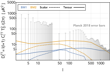
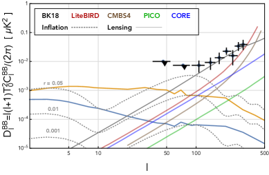
Figure 2: We plot the CMB power spectrum in our setting, saturating the current Planck 2018 bound  Aghanim et al. (2019) (left panel) and show the corresponding B-mode spectra (right panel) for the two benchmark models (see Table. 1). In the left panel we also show the $1\sigma$ error bar of the binned Planck 2018 power spectrum Aghanim et al. (2019) up to $l=2000$ (when $l>2000$ the uncertainty increases) and in the right panel – the measurement from BICEP2/Keck Array Ade et al. (2015a) (digitized from Abazajian et al. (2016)) as well as the projected instrumental noise of several future experiments, including LiteBIRD Hazumi et al. (2019), CMB-S4 Abazajian et al. (2016), PICO Hanany et al. (2019) and CORE Delabrouille et al. (2018) (digitized from Roy et al. (2021)). Additionally, we plot on the right panel the primordial and lensing B-mode spectra for several different tensor-to-scalar ratio $r$ (dotted gray, taken from Hazumi et al. (2019)).

The tensor perturbation $h({\bf k},\tau)$ is obtained from the linear Einstein equation, which is written in terms of $\bar{h}_{ij}=ah_{ij}$ as

$$\bar{h}^{\prime\prime}_{ij}+\left(k^{2}-\frac{a^{\prime\prime}}{a}\right)\bar{h}_{ij}=\dfrac{2}{M^{2}_{Pl}}a\,\Pi_{ij}({\bf k},\tau)\,,$$ (13)

where $\Pi_{ij}({\bf k},\tau)$ is the anisotropic part of the energy momentum tensor $T_{ij}$. The tensor perturbation then generates the B-mode power spectrum as Gorbunov and Rubakov (2011)

$$C^{BB}_{l}= 36\pi\,\mathcal{T}^{2}_{\rm rei}\int\mathcal{D}k\mathcal{D}k^{\prime}\,\mathcal{J}^{2}_{l,B}(k)$$ (14)

$$\cdot\langle\left\{\int^{\tau_{\rm rei}}_{\tau_{\rm rec}}d\tau\,h^{\prime}_{ij}(k,\tau)\dfrac{j_{2}[(\tau_{\rm rei}-\tau)\,k]}{(\tau_{\rm rei}-\tau)^{2}\,k^{2}}\right\}^{2}\rangle\,,$$

where

$$\mathcal{J}_{B,l}(k) =\dfrac{l+2}{2l+1}j_{l-1}(\kappa)-\dfrac{l-1}{2l+1}j_{l+1}(\kappa)\,,$$ (15)

with $\kappa=(\tau_{0}-\tau_{\rm rei})k$. We take the narrow width approximation of the visibility function in time as in the $E$-mode calculation. In contrast to the calculation of $TT$, the $B$-mode signal relies on having the last photon scattering at the reionization. This can be seen by the presence of $j_{2}[(\tau_{\rm rei}-\tau)\,k]$ that comes from expanding the photon propagation within the time interval $[\tau,\tau_{\rm rei}]$ into spherical harmonics and then matching the angular mode to the polarization signal.

As can be seen from Eq. (13), the spectrum $\langle h^{\prime}(k,\tau^{\prime})h^{\prime}(k,\tau^{\prime\prime})\rangle$ is related to $\langle\Pi_{ij}({\bf k},\tau^{\prime})\Pi_{ij}({\bf k^{\prime}},\tau^{\prime\prime})\rangle$, which again can be expressed in terms of the dark photon mode function $v(k,\tau)$. The B-mode spectrum can therefore be rewritten as

$$\begin{aligned} C^{BB}_{l}=&36\pi\,\mathcal{T}^{2}_{\rm rei}\int\mathcal{D}k\int\mathcal{D}k_{1}\Theta(k,k_{1},k_{2})\\ &\cdot\left(B^{2}_{r}(k,k_{1},k_{2})+B^{2}_{i}(k,k_{1},k_{2})\right)\mathcal{J}^{2}_{B,l}(k)\,.\end{aligned}$$ (16)

The function $\Theta$ defined in Eq. (31) comes from the scalar products of the dark photon polarization, while $B_{r}$ and $B_{i}$ are convolutions between $v(k,\tau)$ and the spherical Bessel function $j_{2}$ (see Eq. (32) and Eq. (33)). More details of the derivation appear in Appendix B.

The tensor perturbation also contributes to the $EE$ and $TT$ spectrum. The E-modes have a similar generation mechanism as the B-modes, and we can calculate the $C_{\ell}^{EE}$ by simply replacing $\mathcal{J}_{B,l}(k)$ in Eq. (14) with

$$\begin{aligned} \mathcal{J}_{E,l}(k)=&\dfrac{(l+2)(l+1)}{(2l+1)(2l-1)}j_{l-2}(\kappa)-\dfrac{6(l+2)(l-1)}{(2l+3)(2l-1)}j_{l}(\kappa)\\ &+\dfrac{l(l-1)}{(2l+3)(2l+1)}j_{l+2}(\kappa)\,,\end{aligned}$$ (17)

and the changing the pre-factor from $36\pi$ to $9\pi$. The $TT$ spectrum can be calculated by

$$\begin{split}C^{TT}_{l}&=\dfrac{9\pi}{2}\dfrac{(l+2)!}{(l-2)!}\int\mathcal{D}k\mathcal{D}k^{\prime}\\ &\cdot\langle\left\{\int^{\tau_{0}}_{\tau_{\rm r}}d\tau\,h^{\prime}_{ij}({\bf k},\tau)\dfrac{j_{l}[(\tau_{0}-\tau)k]}{(\tau_{0}-\tau)^{2}k^{2}}\right\}^{2}\rangle\,.\end{split}$$ (18)

As we can see, the power spectra contributed by the tensor and scalar perturbations are proportional $\langle\Pi_{ij}({\bf k},\tau^{\prime})\Pi_{ij}({\bf k^{\prime}},\tau^{\prime\prime})\rangle$, which scales with the mode function of dark photon as $v^{4}$. The energy density of the dark photon field is $\rho_{X}=\frac{1}{2a^{4}}\int\mathcal{D}k\left(\lvert v^{\prime}(k)\rvert^{2}+k^{2}\lvert v(k)\rvert^{2}-k\right)$, where the last term comes from subtracting the vacuum energy Agrawal et al. (2018). When the mode function grows due to the tachyonic production, the axion initial potential energy $\rho_{\phi}=\frac{1}{2}\Lambda^{4}$ quickly transfers into $\rho_{X}$ and generates $v\propto\Lambda^{2}$. When fixing the axion mass $m$ and the axion-dark photon coupling $\alpha$, the magnitude of the resulting spectrum is proportional to $\Lambda^{8}$.

IV Results: The $TT$ and $BB$ spectra

In Fig. 2, we show the $C_{\ell}^{TT}$ and $C_{\ell}^{BB}$ spectra from the two benchmark models defined in Table. 1. In particular, the value of $\Lambda$ is rescaled (keeping $m$ and $\alpha$ fixed) so that the $TT$ spectrum roughly saturates the error bars from the Planck 2018 data Aghanim et al. (2019), as can be seen in the plot. This shows the rough bounds on $\Lambda$ from the current CMB measurements. On the right of Fig. 2 we plot the corresponding $C_{\ell}^{BB}$ signals for the two benchmark models saturating the $C_{\ell}^{TT}$ constraints. This gives the upper range of the predicted B-modes within our setting.

Below we discuss the shape of the calculated spectra. As we can see in Fig. 2 (right), the two axion B-mode curves are roughly parallel to each other. This can be explained by the spherical Bessel function

$$x^{-2}j_{2}(x)\,,\quad x=(\tau_{rei}-\tau)k\,,$$ (19)

from the angular integral that projects the photon polarization tensor to the B-mode perturbation. The function peaks at the origin and is suppressed by $x^{-3}$ when $x\gg 1$, so the integral is dominated by the $k$-modes that minimize $x$. At the same time, the tachyonic production mainly produces $k$-modes larger than $\tau_{rei}^{-1}$. This results in $D_{\ell}^{BB}$ getting most of its contribution from perturbations at $\tau\sim\tau_{rei}$. This explains why the difference in the dark photon production at early times between the two benchmarks does not significantly modify the shape of the $\ell$ spectra even though the axions in the two models start rolling at different times (as shown in Fig. 1).

This behavior does not hold, however, for the $D_{\ell}^{TT}$ spectra which are sensitive to the starting time of the particle production. The $TT$ spectra in Eqs. (11) and (18) are not affected by the reionization and the spherical harmonic projection has the form $j_{\ell}[(\tau_{0}-\tau)k]$, receiving contributions from a wider $\tau$ window for different $\ell$-modes. Our numerical results show that the $TT$ spectra are dominantly contributed by the early period of the dark photon production. This is why they no-longer peak at lower $\ell$-modes as $D_{\ell}^{BB}$, and the peak of the spectrum for the BM1 model, where the particle production starts earlier, is accordingly at higher $\ell$ compared with the peak of the BM2 spectrum.

In the $D_{\ell}^{TT}$ plot, we compare signals from the two benchmark axion models to the Planck 2018 data Aghanim et al. (2019), establishing a rough bound on $\Lambda$. We find that $\Lambda_{\rm bound}\approx 15(9)~{}$meV (see also Table 1) for the BM1 (BM2) that saturates the error bar of the Planck data following the same binning as in Aghanim et al. (2019). We also find a similar sensitivity from the Planck E-mode polarization data, not shown here.

In the $D_{\ell}^{BB}$ plot, we first note that the BICEP2/Keck measurement Ade et al. (2015a) does not exclude the benchmark models. We have accordingly chosen the parameters to satisfy the existing constraints and find that the signal from the late time tachyonic production is well within sensitivities of next-generation CMB B-mode experiments, such as LiteBIRD Hazumi et al. (2019), CMB-S4 Abazajian et al. (2016), PICO Hanany et al. (2019) and CORE Delabrouille et al. (2018).

The B-mode signals from axions peak at low-$\ell$, similarly to those from inflationary tensor modes, in both cases due to reionization. In this region, the inflationary model with $r\sim 0.01$ produces B-mode signals that dominate over the gravitational lensing signal (see e.g. Fig. 1 of Delabrouille et al. (2018)). This suggests that the axion signals can also dominate the lensing background. The scientific goal of LiteBIRD, for example, is to achieve an uncertainty of $\delta r\sim 0.001$ on the range $2\leqslant\ell\leqslant 100$ Hazumi et al. (2019). It has been shown that even with the contamination from diffuse galactic foreground, LiteBIRD can still be sensitive to $D^{BB}_{l}\sim 10^{-4}\mu{\rm K}^{2}$ Campeti et al. (2021) for $\ell\lesssim 10$. Such sensitivity is close to the BM1 signal, and it is also comparable to the BM2 signal even with a lower $\Lambda\approx 7~{}$meV, which is close to the scale of the observed dark energy $\rho_{CC}^{1/4}$. This signal, if observed, might have intriguing implications for the nature of dark energy.

V Conclusion

We have studied the CMB power spectra generated by ALPs via a tachyonic instability and the ensuing production of dark photon quanta close to the cosmic reionization epoch. The ALP-dark photon system produces GWs that leave an imprint in the CMB, including its B-mode polarization spectrum. The signal is visible to future CMB polarization detectors while remaining compatible with the bounds from current measurements. Moreover, we find that future experiments can be sensitive to ALP potential energies similar in order of magnitude to the value of CC, which, if discovered, may lead to progress in discerning the nature of dark energy. We note that our setting may potentially also generate a signal in measures of cosmic non-Gaussianity that could be visible to future experiments. We leave this analysis for a future study.

VI Acknowledgement

We thank Pedro Schwaller, Ben Stefanek, Chen Sun for useful discussions, and especially Gustavo Marques Tavares for useful comments to the draft. MG and SL are supported in part by Israel Science Foundation under Grant No. 1302/19. MG is also supported in part by the US-Israeli BSF grant 2018236 and the GIF grant I-2524-303.7. YT is supported by the NSF grant PHY-2014165. YT was also supported in part by the National Science Foundation under grant PHY-1914731 and by the Maryland Center for Fundamental Physics. The authors also thank the KITP institute (Enervac19 program), and the Munich Institute for Astro- and Particle Physics (MIAPP) of the DFG Excellence Cluster Origins, where part of this work was conducted, for hospitality.

Appendix A Calculation of the CMB $TT$ spectrum

Here we give more details about the $C_{\ell}^{TT}$ calculation from the ISW contribution. We solve the set of differential equations in Eq. (6) by using the Green’s function method and denote the Green’s function for $\Phi$ by $G_{\Phi}(\tau,\tau^{\prime})$, which has the boundary condition of $G_{\Phi}(\tau,\tau)=a(\tau)/(3a^{\prime}(\tau))$. Then for the ISW calculation we should have the conformal time derivative of the gravitational potential $\Phi$ as

$$\Phi^{\prime}(\tau)=G_{\Phi}(\tau,\tau)g({\bf k},\tau)+\int^{\tau}_{\tau_{\rm osc}}d\tau^{\prime}\,\dfrac{dG_{\Phi}(\tau,\tau^{\prime})}{d\tau}g({\bf k},\tau^{\prime})\,,$$ (20)

where we have defined $g({\bf k},\tau)\equiv-4\pi G_{N}\,a^{2}\delta\rho_{e}$ for convenience. With the $d\tau$ integration in Eq. (9), we reorganize the expression by switching the order of the conformal time integrals as

$$\tilde{\Theta}_{l}({\bf k}) =2\int^{\tau_{0}}_{\tau_{\rm osc}}d\tau\,G_{\Phi}(\tau,\tau)g({\bf k},\tau)j_{l}[k(\tau_{0}-\tau)]+2\int^{\tau_{0}}_{\tau_{\rm osc}}d\tau\int^{\tau}_{\tau_{\rm osc}}d\tau^{\prime}\dfrac{dG_{\Phi}(\tau,\tau^{\prime})}{d\tau}g({\bf k},\tau^{\prime})j_{l}[k(\tau_{0}-\tau)]$$ (21)

$$=2\int^{\tau_{0}}_{\tau_{\rm osc}}d\tau G_{\Phi}(\tau,\tau)g({\bf k},\tau)j_{l}[k(\tau_{0}-\tau)]+2\int^{\tau_{0}}_{\tau_{\rm osc}}d\tau^{\prime}\int^{\tau_{0}}_{\tau^{\prime}}d\tau\dfrac{dG_{\Phi}(\tau,\tau^{\prime})}{d\tau}g({\bf k},\tau^{\prime})j_{l}[k(\tau_{0}-\tau)]$$ (22)

$$=2\int^{\tau_{0}}_{\tau_{\rm osc}}d\tau^{\prime}\left\{G_{\Phi}(\tau^{\prime},\tau^{\prime})j_{l}[k(\tau_{0}-\tau^{\prime})]+\int^{\tau_{0}}_{\tau^{\prime}}d\tau\,\dfrac{dG_{\Phi}(\tau,\tau^{\prime})}{d\tau}j_{l}[k(\tau_{0}-\tau)]\right\}g({\bf k},\tau^{\prime})$$ (23)

$$=2\int^{\tau_{0}}_{\tau_{\rm osc}}d\tau^{\prime}\,f_{T,l}(k,\tau^{\prime})g({\bf k},\tau^{\prime})\,.$$ (24)

We can then convert the correlation function $\langle\tilde{\Theta}_{l}({\bf k})\tilde{\Theta}_{l}({\bf k^{\prime}})\rangle$ into $\langle\delta\rho_{e}({\bf k},\tau)\delta\rho_{e}({\bf k^{\prime}},\tau^{\prime})\rangle$. The $\delta\rho_{e}$ operator can be expressed with the dark photon fields by replacing the $X_{i}$ and $X_{ij}$ in Eq. (7) with the definitions in Eq. (3), and its spectrum is obtained as $\langle 0|\delta\left[\mathcal{O}\right]\delta\left[\mathcal{O}\right]|0\rangle=\langle 0|\mathcal{O}^{2}|0\rangle-\langle 0|\mathcal{O}|0\rangle^{2}$. After a lengthy but straightforward calculation one arrives at Eq. (11). The expression of the function $T^{r}_{\ell}$ and $T^{i}_{\ell}$ are

$$T^{r}_{\ell}(k,k_{1},k_{2}) =\int^{\tau_{0}}_{\tau_{\rm osc}}d\tau\dfrac{1}{a^{2}(\tau)}f_{T,l}(k,\tau){\rm Re}\left\{v_{+}(\tau,k_{1})v_{+}(\tau,k_{2})+\dfrac{v^{\prime}_{+}(\tau,k_{1})v^{\prime}_{+}(\tau,k_{2})}{k_{1}k_{2}}\right\}\,,$$ (25)

$$T^{i}_{\ell}(k,k_{1},k_{2}) =\int^{\tau_{0}}_{\tau_{\rm osc}}d\tau\dfrac{1}{a^{2}(\tau)}f_{T,l}(k,\tau){\rm Im}\left\{v_{+}(\tau,k_{1})v_{+}(\tau,k_{2})+\dfrac{v^{\prime}_{+}(\tau,k_{1})v^{\prime}_{+}(\tau,k_{2})}{k_{1}k_{2}}\right\}\,.$$ (26)

Appendix B Calculation of the CMB B-mode spectrum

The solution to Eq. (13) can be written as

$$\bar{h}_{ij}({\bf k},\tau)=\dfrac{2}{M^{2}_{Pl}}\int^{\tau}_{\tau_{\rm osc}}d\tau^{\prime}a(\tau^{\prime})G(k,\tau,\tau^{\prime})\Pi_{ij}({\bf k},\tau^{\prime}),$$ (27)

where $G$ is the Green’s function which solves $d^{2}G/d\tau^{2}+\left(k^{2}-a^{\prime\prime}/a\right)G=\delta(\tau-\tau^{\prime})$, and satisfies $G(\tau<\tau^{\prime})=0$, $G(k,\tau,\tau)=0$ and $G^{\prime}(k,\tau,\tau)=1$. With this expression, the spectrum $\langle h^{\prime}_{ij}({\bf k},\tau_{1})h^{\prime}_{ij}({\bf k},\tau_{2})\rangle$ is converted to $\Pi^{2}({\bf k},\tau^{\prime}_{1},\tau^{\prime}_{2})$, where $\Pi^{2}({\bf k},\tau^{\prime}_{1},\tau^{\prime}_{2})$ is defined as $\langle\Pi_{ij}({\bf k},\tau)\Pi_{ij}({\bf k^{\prime}},\tau^{\prime})\rangle=(2\pi)^{3}\Pi^{2}({\bf k},\tau,\tau^{\prime})\delta({\bf k}+{\bf k^{\prime}})$ . Using the results in Ref. Machado et al. (2019a), $\Pi^{2}({\bf k},\tau,\tau^{\prime})$ can be expressed as

$$\Pi^{2}({\bf k},\tau,\tau^{\prime})=2\int\mathcal{D}q\,\Theta_{++}({\bf k}-{\bf q},{\bf k})\mathcal{S}_{++}({\bf q},{\bf k},\tau)\mathcal{S}^{*}_{++}({\bf q},{\bf k},\tau^{\prime})\,,$$ (28)

where the subscript ++ means we include only the positive helicity (which dominates over the negative helicity). The function $\Theta$ and $\mathcal{S}$ are also explicitly given in Ref. Machado et al. (2019a) as

$$\lvert\Theta_{++}({\bf q},{\bf k})\rvert^{2} =\dfrac{1}{16}\left[\left(1+\dfrac{{\bf k}\cdot{\bf q}}{\lvert{\bf k}\rvert\,\lvert{\bf q}\rvert}\right)^{2}\left(1+\dfrac{{\bf k}\cdot({\bf k}-{\bf q})}{\lvert{\bf k}\rvert\,\lvert{\bf k}-{\bf q}\rvert}\right)^{2}+\left(1-\dfrac{{\bf k}\cdot{\bf q}}{\lvert{\bf k}\rvert\,\lvert{\bf q}\rvert}\right)^{2}\left(1-\dfrac{{\bf k}\cdot({\bf k}-{\bf q})}{\lvert{\bf k}\rvert\,\lvert{\bf k}-{\bf q}\rvert}\right)^{2}\right]\,,$$ (29)

$$\mathcal{S}_{++}({\bf q},{\bf k},\tau) =-\dfrac{1}{a^{2}(\tau)}\left[\lvert{\bf q}\rvert\lvert{\bf k}-{\bf q}\rvert v_{+}({\bf q},\tau)v_{+}({\bf k}-{\bf q},\tau)+v^{\prime}_{+}({\bf q},\tau)v^{\prime}_{+}({\bf k}-{\bf q},\tau)\right]\,.$$ (30)

These give us all the ingredients for the $C^{BB}_{l}$ calculation. Putting all the explicit expressions back to Eq. (14), and using the same trick as in the calculation of $C^{TT}_{l}$ to switch the sequence of the two conformal time integrals $\int_{\tau_{\rm osc}}^{\tau_{\rm rei}}d\tau\int_{\tau_{\rm osc}}^{\tau}d\tau^{\prime}\to\int_{\tau_{\rm osc}}^{\tau_{\rm rei}}d\tau^{\prime}\int_{\tau^{\prime}}^{\tau_{\rm rei}}d\tau$ involved in Eq. (14), we arrive at the result Eq. (16) after a simplification. The functions involved in the final expression Eq. (16) are defined as

$$\Theta(a,b,c) =\dfrac{1}{16}\left[\dfrac{\left((a+b)^{2}-c^{2}\right)^{2}}{4a^{2}b^{2}}\dfrac{\left((a+c)^{2}-b^{2}\right)}{4a^{2}c^{2}}+\dfrac{\left((a-b)^{2}-c^{2}\right)^{2}}{4a^{2}b^{2}}\dfrac{\left((a-c)^{2}-b^{2}\right)}{4a^{2}c^{2}}\right],$$ (31)

$$B_{r}(k,k_{1},k_{2}) =\dfrac{2}{M_{\rm pl}^{2}}\int^{\tau_{\rm rei}}_{\tau_{\rm osc}}d\tau\dfrac{1}{a^{2}(\tau)}f_{B}(k,\tau)\,{\rm Re}\left\{v^{\prime}_{+}(\tau,k_{1})v^{\prime}_{+}(\tau,k_{2})+k_{1}k_{2}v_{+}(\tau,k_{1})v_{+}(\tau,k_{2})\right\},$$ (32)

$$B_{i}(k,k_{1},k_{2}) =\dfrac{2}{M_{\rm pl}^{2}}\int^{\tau_{\rm rei}}_{\tau_{\rm osc}}d\tau\dfrac{1}{a^{2}(\tau)}f_{B}(k,\tau)\,{\rm Im}\left\{v^{\prime}_{+}(\tau,k_{1})v^{\prime}_{+}(\tau,k_{2})+k_{1}k_{2}v_{+}(\tau,k_{1})v_{+}(\tau,k_{2})\right\},$$ (33)

$$f_{B}(k,\tau) =\int^{\tau_{\rm rei}}_{\tau}d\tau^{\prime}\dfrac{1}{a(\tau^{\prime})}\mathcal{G}(k,\tau^{\prime},\tau)\dfrac{j_{2}[(\tau_{\rm rei}-\tau^{\prime})k]}{(\tau_{\rm rei}-\tau^{\prime})^{2}k^{2}},$$ (34)

where $\mathcal{G}(k,\tau,\tau^{\prime})\equiv dG(k,\tau,\tau^{\prime})/d\tau-a^{\prime}(\tau)/a(\tau)G(k,\tau,\tau^{\prime})$.

References

- Aasi et al. (2015) J. Aasi, B. Abbott, R. Abbott, T. Abbott, M. Abernathy, K. Ackley, C. Adams, T. Adams, P. Addesso, R. Adhikari, et al., Classical and quantum gravity 32, 074001 (2015).
- Acernese et al. (2014) F. Acernese, M. Agathos, K. Agatsuma, D. Aisa, N. Allemandou, A. Allocca, J. Amarni, P. Astone, G. Balestri, G. Ballardin, et al., Classical and Quantum Gravity 32, 024001 (2014).
- Caprini et al. (2020) C. Caprini et al., JCAP 03, 024 (2020), arXiv:1910.13125 [astro-ph.CO] .
- Auclair et al. (2020) P. Auclair et al., JCAP 04, 034 (2020), arXiv:1909.00819 [astro-ph.CO] .
- Geller et al. (2018) M. Geller, A. Hook, R. Sundrum, and Y. Tsai, Phys. Rev. Lett. 121, 201303 (2018), arXiv:1803.10780 [hep-ph] .
- Cui et al. (2018) Y. Cui, M. Lewicki, D. E. Morrissey, and J. D. Wells, Phys. Rev. D 97, 123505 (2018), arXiv:1711.03104 [hep-ph] .
- Kawamura et al. (2011) S. Kawamura et al., Class. Quant. Grav. 28, 094011 (2011).
- Amaro-Seoane et al. (2017) P. Amaro-Seoane et al., ArXiv e-prints (2017), arXiv:1702.00786 [astro-ph.IM] .
- Punturo et al. (2010) M. Punturo et al., Class. Quant. Grav. 27, 194002 (2010).
- Crowder and Cornish (2005) J. Crowder and N. J. Cornish, Phys. Rev. D 72, 083005 (2005), arXiv:gr-qc/0506015 .
- Dewdney et al. (2009) P. E. Dewdney, P. J. Hall, R. T. Schilizzi, and T. J. L. Lazio, Proceedings of the IEEE 97, 1482 (2009).
- Manchester (2013) R. Manchester, Classical and Quantum Gravity 30, 224010 (2013).
- Ade et al. (2015a) P. A. R. Ade et al. (BICEP2, Keck Array), Astrophys. J. 811, 126 (2015a), arXiv:1502.00643 [astro-ph.CO] .
- Kamionkowski and Kovetz (2016) M. Kamionkowski and E. D. Kovetz, Ann. Rev. Astron. Astrophys. 54, 227 (2016), arXiv:1510.06042 [astro-ph.CO] .
- Peccei and Quinn (1977a) R. Peccei and H. R. Quinn, Phys. Rev. Lett. 38, 1440 (1977a).
- Peccei and Quinn (1977b) R. Peccei and H. R. Quinn, Phys. Rev. D 16, 1791 (1977b).
- Abbott and Sikivie (1983) L. Abbott and P. Sikivie, Phys. Lett. B 120, 133 (1983).
- Preskill et al. (1983) J. Preskill, M. B. Wise, and F. Wilczek, Phys. Lett. B 120, 127 (1983).
- Dine and Fischler (1983) M. Dine and W. Fischler, Phys. Lett. B 120, 137 (1983).
- Co et al. (2018) R. T. Co, L. J. Hall, and K. Harigaya, Phys. Rev. Lett. 120, 211602 (2018), arXiv:1711.10486 [hep-ph] .
- Freese et al. (1990) K. Freese, J. A. Frieman, and A. V. Olinto, Phys. Rev. Lett. 65, 3233 (1990).
- Dimopoulos et al. (2008) S. Dimopoulos, S. Kachru, J. McGreevy, and J. G. Wacker, JCAP 08, 003 (2008), arXiv:hep-th/0507205 .
- Anber and Sorbo (2010) M. M. Anber and L. Sorbo, Phys. Rev. D 81, 043534 (2010), arXiv:0908.4089 [hep-th] .
- Hook and Marques-Tavares (2016) A. Hook and G. Marques-Tavares, JHEP 12, 101 (2016), arXiv:1607.01786 [hep-ph] .
- Fonseca et al. (2020) N. Fonseca, E. Morgante, R. Sato, and G. Servant, JHEP 04, 010 (2020), arXiv:1911.08472 [hep-ph] .
- Graham et al. (2015) P. W. Graham, D. E. Kaplan, and S. Rajendran, Phys. Rev. Lett. 115, 221801 (2015), arXiv:1504.07551 [hep-ph] .
- Anastassopoulos et al. (2017) V. Anastassopoulos et al. (CAST), Nature Phys. 13, 584 (2017), arXiv:1705.02290 [hep-ex] .
- Du et al. (2018) N. Du et al. (ADMX), Phys. Rev. Lett. 120, 151301 (2018), arXiv:1804.05750 [hep-ex] .
- Ouellet et al. (2019) J. L. Ouellet et al., Phys. Rev. Lett. 122, 121802 (2019), arXiv:1810.12257 [hep-ex] .
- Zhong et al. (2018) L. Zhong et al. (HAYSTAC), Phys. Rev. D 97, 092001 (2018), arXiv:1803.03690 [hep-ex] .
- Liu et al. (2019) H. Liu, B. D. Elwood, M. Evans, and J. Thaler, Phys. Rev. D 100, 023548 (2019), arXiv:1809.01656 [hep-ph] .
- Bogorad et al. (2019) Z. Bogorad, A. Hook, Y. Kahn, and Y. Soreq, Phys. Rev. Lett. 123, 021801 (2019), arXiv:1902.01418 [hep-ph] .
- Hook et al. (2018) A. Hook, Y. Kahn, B. R. Safdi, and Z. Sun, Phys. Rev. Lett. 121, 241102 (2018), arXiv:1804.03145 [hep-ph] .
- Caputo et al. (2019) A. Caputo, M. Regis, M. Taoso, and S. J. Witte, JCAP 03, 027 (2019), arXiv:1811.08436 [hep-ph] .
- Anber and Sorbo (2012) M. M. Anber and L. Sorbo, Phys. Rev. D 85, 123537 (2012), arXiv:1203.5849 [astro-ph.CO] .
- Co et al. (2019) R. T. Co, A. Pierce, Z. Zhang, and Y. Zhao, Phys. Rev. D 99, 075002 (2019), arXiv:1810.07196 [hep-ph] .
- Agrawal et al. (2018) P. Agrawal, G. Marques-Tavares, and W. Xue, JHEP 03, 049 (2018), arXiv:1708.05008 [hep-ph] .
- Machado et al. (2019a) C. S. Machado, W. Ratzinger, P. Schwaller, and B. A. Stefanek, JHEP 01, 053 (2019a), arXiv:1811.01950 [hep-ph] .
- Machado et al. (2019b) C. S. Machado, W. Ratzinger, P. Schwaller, and B. A. Stefanek, (2019b), arXiv:1912.01007 [hep-ph] .
- Weiner et al. (2021) Z. J. Weiner, P. Adshead, and J. T. Giblin, Phys. Rev. D 103, L021301 (2021), arXiv:2008.01732 [astro-ph.CO] .
- Bernal et al. (2016) J. L. Bernal, L. Verde, and A. G. Riess, JCAP 10, 019 (2016), arXiv:1607.05617 [astro-ph.CO] .
- Poulin et al. (2019) V. Poulin, T. L. Smith, T. Karwal, and M. Kamionkowski, Phys. Rev. Lett. 122, 221301 (2019), arXiv:1811.04083 [astro-ph.CO] .
- Aghanim et al. (2019) N. Aghanim et al. (Planck), (2019), arXiv:1907.12875 [astro-ph.CO] .
- Ade et al. (2015b) P. A. R. Ade et al. (BICEP2, Planck), Phys. Rev. Lett. 114, 101301 (2015b), arXiv:1502.00612 [astro-ph.CO] .
- Graham et al. (2019) P. W. Graham, D. E. Kaplan, and S. Rajendran, Phys. Rev. D 100, 015048 (2019), arXiv:1902.06793 [hep-ph] .
- Ratzinger et al. (2020) W. Ratzinger, P. Schwaller, and B. A. Stefanek, (2020), arXiv:2012.11584 [astro-ph.CO] .
- Kitajima et al. (2018) N. Kitajima, T. Sekiguchi, and F. Takahashi, Phys. Lett. B 781, 684 (2018), arXiv:1711.06590 [hep-ph] .
- Agrawal et al. (2020) P. Agrawal, N. Kitajima, M. Reece, T. Sekiguchi, and F. Takahashi, Phys. Lett. B 801, 135136 (2020), arXiv:1810.07188 [hep-ph] .
- Kitajima et al. (2020) N. Kitajima, J. Soda, and Y. Urakawa, (2020), arXiv:2010.10990 [astro-ph.CO] .
- Ma and Bertschinger (1995) C.-P. Ma and E. Bertschinger, Astrophys. J. 455, 7 (1995), arXiv:astro-ph/9506072 .
- Gorbunov and Rubakov (2011) D. S. Gorbunov and V. A. Rubakov, Introduction to the theory of the early universe: Cosmological perturbations and inflationary theory (World Scientific, 2011).
- Abazajian et al. (2016) K. N. Abazajian et al. (CMB-S4), (2016), arXiv:1610.02743 [astro-ph.CO] .
- Hazumi et al. (2019) M. Hazumi et al., J. Low Temp. Phys. 194, 443 (2019).
- Hanany et al. (2019) S. Hanany et al. (NASA PICO), (2019), arXiv:1902.10541 [astro-ph.IM] .
- Delabrouille et al. (2018) J. Delabrouille et al. (CORE), JCAP 04, 014 (2018), arXiv:1706.04516 [astro-ph.IM] .
- Roy et al. (2021) A. Roy, G. Kulkarni, P. D. Meerburg, A. Challinor, C. Baccigalupi, A. Lapi, and M. G. Haehnelt, JCAP 01, 003 (2021), arXiv:2004.02927 [astro-ph.CO] .
- Campeti et al. (2021) P. Campeti, E. Komatsu, D. Poletti, and C. Baccigalupi, JCAP 01, 012 (2021), arXiv:2007.04241 [astro-ph.CO] .