Divide-and-Conquer for Lane-Aware Diverse Trajectory Prediction

Abstract

Trajectory prediction is a safety-critical tool for autonomous vehicles to plan and execute actions. Our work addresses two key challenges in trajectory prediction, learning multimodal outputs, and better predictions by imposing constraints using driving knowledge. Recent methods have achieved strong performances using Multi-Choice Learning objectives like winner-takes-all (WTA) or best-of-many. But the impact of those methods in learning diverse hypotheses is under-studied as such objectives highly depend on their initialization for diversity. As our first contribution, we propose a novel Divide-And-Conquer (DAC) approach that acts as a better initialization technique to WTA objective, resulting in diverse outputs without any spurious modes. Our second contribution is a novel trajectory prediction framework called ALAN that uses existing lane centerlines as anchors to provide trajectories constrained to the input lanes. Our framework provides multi-agent trajectory outputs in a forward pass by capturing interactions through hypercolumn descriptors and incorporating scene information in the form of rasterized images and per-agent lane anchors. Experiments on synthetic and real data show that the proposed DAC captures the data distribution better compare to other WTA family of objectives. Further, we show that our ALAN approach provides on par or better performance with SOTA methods evaluated on Nuscenes urban driving benchmark.

1 Introduction

Prediction of diverse multimodal behaviors is a critical need to proactively make safe decisions for autonomous vehicles. A major challenge lies in predicting not only the most dominant modes but also accounting for the less dominant ones that might arise sporadically. Hence, there is need for models that can disentangle the plausible output space and provide diverse futures for any given number of samples. Further, a vast majority of actors execute socially acceptable maneuvers that adhere with the underlying scene structure. Predicting socially non-viable outputs can lead to unsafe planning decisions with some more dangerous than the others [7]. For example, a method that provides close enough predictions that does not follow road semantics is more dangerous compared to similar performing method that adheres to the scene structure.

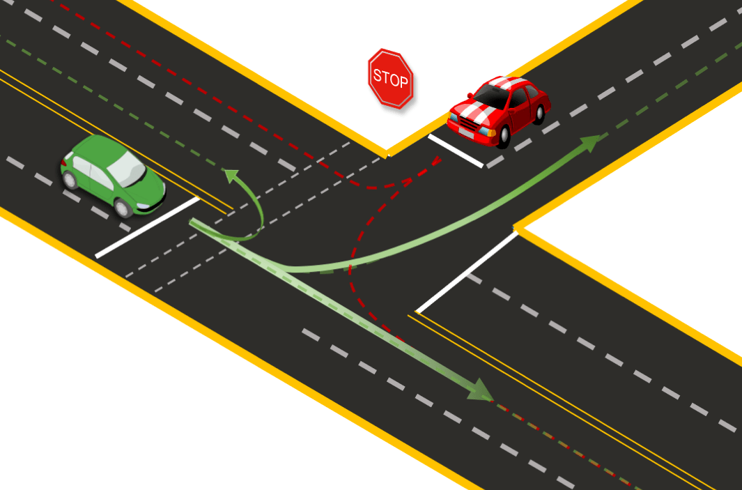
Figure 1: Depicts trajectory prediction problem in an intersection scenario with possible lane anchors for agents shown as coloured dashed lines.

Traditionally, generative models have been widely adapted to capture the uncertainties related to trajectory prediction problems [29, 24, 42, 23, 44]. However, generative methods may suffer from mode collapse issues, which reduces their applicability for safety critical applications such as self-driving cars. Recent methods [36, 32] use Multi-Choice Learning objectives [30] like winner-takes-all (WTA) but suffer from instability associated with network initialization [34, 39]. As a first contribution, we propose a Divide and Conquer (DAC) approach that provides a better initialization to the WTA objective. Our method solves issues related to spurious modes where some hypotheses are either untrained in the training process, or reach equilibrium positions that do not represent any part of the data. We show that the proposed DAC captures the data distribution better on both real and synthetic scenes with multi-modal ground truth, compared to baseline WTA objectives [34, 39].

Further, trajectory prediction methods incorporate driving knowledge using scene context either in the form of rasterized images [29, 42, 44, 36, 38, 8] or by exploiting HD map data structure [32, 17] as inputs. Usually, this information is represented as a feature given as input to the network and does not guarantee strong semantic coupling. Our second contribution addresses this by proposing ALAN, a novel trajectory prediction framework that uses lane centerlines as anchors to predict trajectories (Figure 1). Our outputs provide accurate predictions with strong semantic alignment demonstrated by FDE and OffRoadRate values and validated using our qualitative visualizations.

Specifically, we use a single representational model [44] for multi-agent inputs and encode interactions through novel use of hypercolumn descriptors [2] that extracts information from features at multiple scales. Moreover, we transform the prediction problem to normal-tangential ($nt$) coordinates with respect to input lanes. This is critical in order to use lane centerlines as anchors. Further, we regularize anchor outputs through auxiliary $xy$ predictions to make them less susceptible to bad anchors and rely on agent dynamics. Finally, we rank our predictions through an Inverse Optimal Control based ranking module [29].

In summary, our contributions are the following:

• A novel Divide and Conquer approach as a better initialization to WTA objective that captures data distribution without any spurious modes.

• A new anchor based trajectory prediction framework called ALAN that uses existing centerlines as anchors to provide context-aware outputs with strong semantic coupling.

• Strong empirical performance on the Nuscenes urban driving benchmark.

2 Related Work

Multi-Choice Learning: Multi-modal predictions have been realized in different domains through Multi-choice learning (MCL) [19, 13, 30] objectives in the past. Several works have shown use cases of MCL to provide diverse hypotheses in classification [30, 39], segmentation [30, 39], captioning [30], pose estimation [39], image synthesis [11] and trajectory proposals [45]. Convergence issue related to WTA objectives have been shown in [39, 34]. Following this work, [39] proposed a relaxed winner-takes-all objective (RWTA) to solve the convergence problem but this method itself suffers from the problem of hypotheses incorrectly capturing the data distribution. [34] proposed an evolving winner-takes-all (EWTA) loss that captures the distribution better compared to [39]. Despite the aforementioned improvements, these methods still can’t capture the data distribution accurately due to spurious modes at equilibrium or hypotheses untrained during the training process. Alternatively, we propose a Divide and Conquer approach where we exponentially increase the effective number of outputs during training with set of hypotheses capturing some part of the data at every stage.

Forecasting Methods: The future trajectory prediction has been investigated broadly in the literature using both classical [47, 31, 27] and deep learning based methods [18, 1, 44]. Deterministic models [1, 33, 41] predict most likely trajectory for each agent in the scene while neglecting the uncertainties inherited in the trajectory prediction problem. To capture the uncertainties and create diverse trajectory predictions, stochastic methods have been proposed which encode possible modes of future trajectories through sampling random variables. Non-parametric deep generative models such as Conditional Variational Autoencoder (CVAE) [29, 3, 24, 22, 44] and Generative Adversarial Networks (GANs) [28, 18, 40] have been widely used in this domain. However, these methods fail to capture all underlying modes due to imbalance in the latent distribution [48]. Recent methods predict a fixed set of diverse trajectories [36, 32] for the same input context. Our method uses a similar approach to predict a set of $M$ hypothesis.

Representation: HD map rasterization have been widely used in the literature to encode and process map information by neural networks [3, 51, 14, 6, 44]. Some methods [43, 35] construct top view map using semantics and depth information from perspective images. Some [49, 6] use a combination rasterzied HD maps and sensor information. Several recent works [32, 17] utilize map information directly by representing the vectorized map data as a graph data structure. Our work uses a hybrid map input combining both rasterized map and vectorized lane data provided as input for every agent at its location on the spatial grid [44].

Trajectory Prediction: Traditionally, several works [44, 32, 17, 36] formulate trajectory prediction problem as a regression over cartesian coordinates. [43] poses it as a classification of future locations over a spatial grid. Chang et. al [9] use a normal-tangential coordinate similar to ours but is only limited to classical nearest neighbor and vanilla LSTM [21] approaches. Related to our work, some methods tackle the multi-modality problem by quantizing the output space into several predefined diverse anchors and then reformulating the original trajectory problem into sequential anchor classification (selection) and offset regression sub-problems [50, 38, 8, 49]. However, Anchors usually are pre-clustered into a fixed set as a priori or are calculated in real-time based on kinematic heuristics [50]. Hence, the process of creating anchors may add computational complexity in the inference time, also it could be highly scenario dependent and hard to generalize. In contrast, our method uses HD map centerline information as anchors which is consistent for diverse scenarios and also readily available at inference.

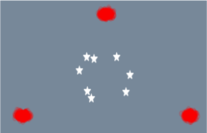
(a) Init

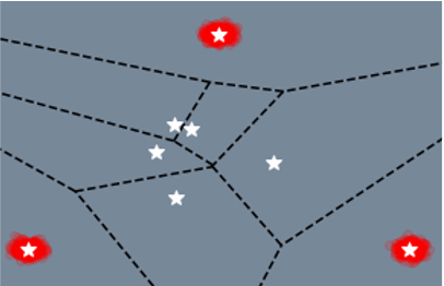
(b) WTA

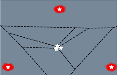
(c) RWTA

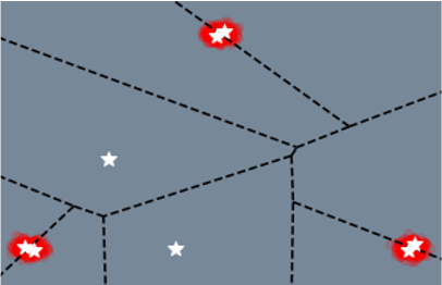
(d) EWTA

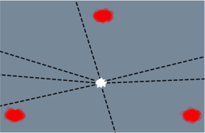
(e) DAC - Depth 1

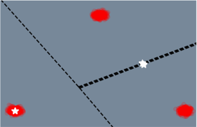
(f) DAC - Depth 2

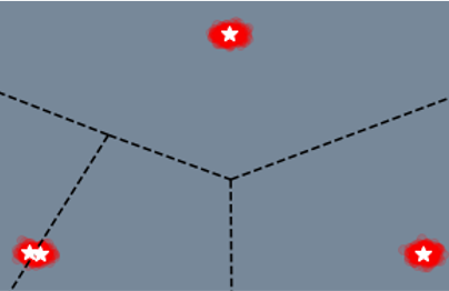
(g) DAC - Depth 3

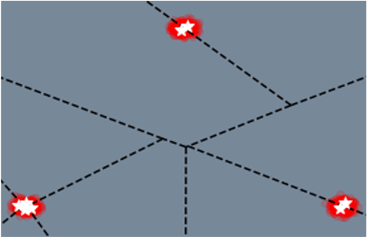
(h) DAC - Depth 4

Figure 2: Toy example comparing different versions of winner-takes-all and enclosed voronoi regions of their predicted hypotheses. The toy data is shown in red and the hypotheses are shown in white. With Depth=1 for DAC, it contains a single set with $M$ hypotheses, thus all hypotheses are penalized to match the data and reach the equilibrium. As the depth increases the number of sets in the list grows exponentially as every set is broken down into halves ($e\xrightarrow[]{}f\xrightarrow{}g\xrightarrow{}h$). Since we show the same ground truths to all the hypotheses in a set, they reach the same equilibrium position forming centroidal voronoi tessellation with number of outputs effectively equal to the number of sets in the list ($e\xrightarrow{}1,f\xrightarrow{}2,g\xrightarrow{}4,h\xrightarrow{}8$). In the final stage (h), every set contains one hypothesis resembling a WTA objective. In comparison to DAC, other WTA objectives model the data distribution incorrectly since some Voronoi regions do not capture any part of the data, resulting in spurious modes.

3 Divide and Conquer

In this section, we provide detailed description of our method in training Multi-Hypothesis prediction networks where our approach acts as an initialization technique for winner-takes-all [30] objective. Let $\mathcal{X}$ denote the vector space of inputs and $\mathcal{Y}$ denotes the vector space of output variables. Let $\mathcal{D}=\{(x_{i},y_{i}),...,(x_{N},y_{N})\}$ be a set of $N$ training tuples and $p(x,y)=p(y|x)p(x)$ be the joint probability density. Our goal is to learn a function $f_{\theta}:\mathcal{X}\xrightarrow{}\mathcal{Y}^{M}$ that maps every input in $\mathcal{X}$ to a set of $M$ hypotheses. Mathematically, we define:

$$f_{\theta}(x)=(f_{\theta}^{1}(x),...,f_{\theta}^{M}(x)).$$ (1)

As shown by Rupprecht et al. [39], winner-takes-all objective minimizes the loss with the closest of $M$ hypotheses:

$$\int_{\mathcal{X}}\sum_{j=1}^{M}\int_{\mathcal{Y}_{j(x)}}\mathcal{L}(f_{\theta}^{j}(x),y)p(x,y)dydx,$$ (2)

where $\mathcal{Y}_{j}$ is the Voronoi tessellation of label space with $\mathcal{Y}=\cup_{j=1}^{M}\mathcal{Y}_{j}$. This objective leads to Centroidal Voronoi tessellation [15] of outputs where each hypothesis minimizes to the probabilistic mass centroid of the Voronoi label space $\mathcal{Y}_{j}$ enclosed by it. In practice, to obtain diverse hypotheses WTA objective can be written as a meta loss [34, 39, 30, 19],

$$\mathcal{L}_{WTA}=\sum_{k=1}^{K}\delta_{k}(k==\operatorname*{arg\,min}_{i}\mathcal{L}(f_{\theta}^{i}))\mathcal{L}(f_{\theta}^{k}(x),y),$$ (3)

where $\delta(\cdot)$ is the Kronecker delta function with value 1 when condition is True and 0 otherwise.

Initialization difficulties for WTA

As mentioned by Makansi et al. [34] Equation 3 can be compared to EM algorithm and K-means clustering where they depend mainly on initialization for optimal convergence. As shown in 2(b) this makes training process very brittle as the Voronoi region of only few hypotheses encloses the data distribution, leaving most of the hypotheses untrained due to winner-takes-all objective. The alternative solution proposed by Ruppercht et al. [39] to solve the convergence problem by assigning $\epsilon$ weight to the non-winners does not work as every ground truth associates with atmost one hypothesis making other non-winners to reach the equilibrium as shown in 2(c). Makansi et. al, [34] then proposed evolving winner-takes-all (EWTA) objective where they update top $k$ winners. The $k$ varies starting from $k=M$ to $k=1$ leading to winner takes all objective in training process. This method captures the data distribution better compared to RWTA and WTA but still produces hypothesis with incorrect modes as shown in the Figure 2(d).

DAC for diverse non-spurious modes

We propose an novel initialization technique called Divide and Conquer that alleviates the problem of spurious modes, leaving the Voronoi region of every output hypothesis to capture some part of the data, as shown in Figure 2(h). We divide $M$ hypotheses into $k$ sets and update the set with argmin outputs to match the ground truth. The value of $k$ starts with $1$ and increases exponentially as every set is broken down into two halves as we progress through the training. This creates a binary tree with the depth of the tree dependent on the number of output hypotheses $M$. Algorithm 1 shows pseudo-code of the proposed Divide and Conquer technique. Here depth specifies the maximum depth that can be reached in the current training stage and we define list as variable containing set of hypotheses at any stage in the training. Further, we define newly formed sets from $k^{th}$ set as $set_{k1}$ and $set_{k2}$. Set from the list that produces argmin output is denoted as mSet. Finally we take mean loss of all hypotheses in mSet to get $\mathcal{L}_{DAC}$.

From Figure 2(e), with $k=1$ and list containing a single set, all $M$ hypotheses reach towards the equilibrium. As the number of sets in the list increases from 2(e) to 2(f) the hypotheses divide the distribution space based on the Voronoi region to capture different parts of the data. The effective number of outputs grows at every stage, with the data captured by the $k^{th}$ set in the previous stage split across two newly formed sets in the next stage. Finally, as we reach the leaf nodes, every set contains one hypothesis leading to a winner-takes-all objective similar to Equation 3.

DAC starts with all hypotheses fitting the whole data and at every stage DAC ensures some data to be enclosed in the Voronoi space. During split, hypotheses divide the data enclosed within their Voronoi space to reach new equilibrium. Although, DAC does not guarantee equal number of hypotheses capturing different modes of the data it ensures convergence. Further we would like to note that DAC does not have any significant computational complexity as only dividing into sets and min calculations are involved. In Section 5, we show benefits of DAC in capturing multimodal distributions better, producing diverse set of hypotheses compared to other WTA objectives.

Algorithm 1 Divide and Conquer technique

1:procedure DAC(loss, depth)

2:     $set_{1}=$ $\{$loss$\}$ $\triangleright$ All M hypotheses

3:     list = [$set_{1}$]

4:     for $i\leftarrow 2$ to depth do

5:         for $set_{k}\in\texttt{list}$ do

6:              $\sslash$ Divide $set_{k}$ into halves

7:              list $+=[\{set_{k1}\},\{set_{k2}\}]$               

8:     $\texttt{mSet}=\{$ $set_{k}:\min(set_{k})<\min(set_{j});\forall j\in\{1..len(\texttt{list})\},j\not=k\}$

9:     $\mathcal{L}_{DAC}=mean(\texttt{mSet})$

10:     return $\mathcal{L}_{DAC}$

4 Trajectory Prediction with Lane Anchors

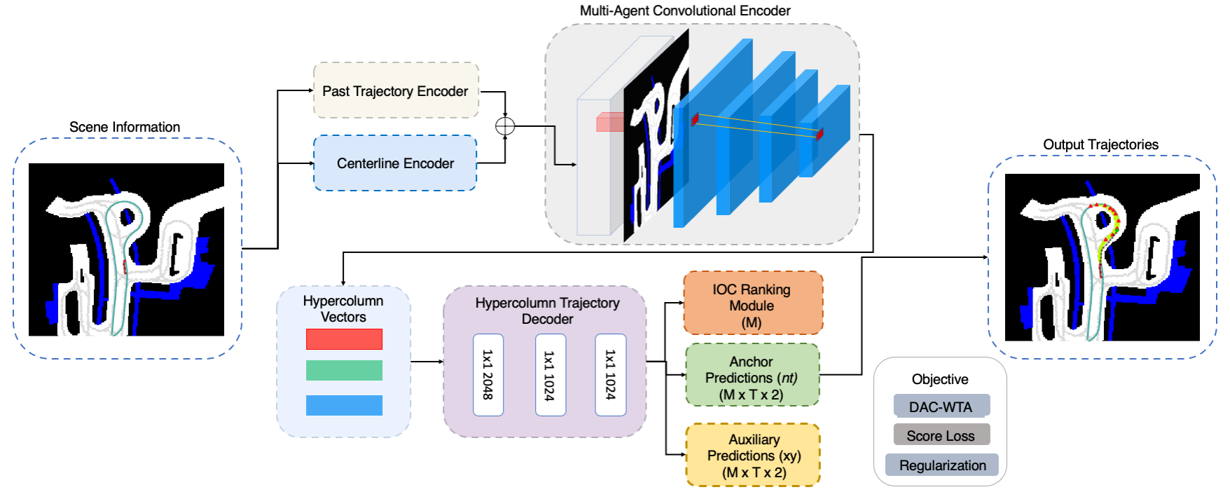
Figure 3: Overview of our proposed ALAN approach. The method takes in past trajectory along with lane anchor and BEV map as input to provide multi-hypothesis predictions for all agents at once.

In this section, we introduce a single representation model called ALAN that produces lane aware trajectories for multiple agents in a forward pass. We formulate the problem as one shot regression of diverse hypotheses across time steps. We now describe our method in detail.

4.1 Problem Statement

Our method takes scene context input in two forms: a) rasterized birds-eye-view (BEV) representation of the scene denoted as ${\bf I}$ of size $H\times W\times 3$ and b) per-agent lane centerline information as anchors. We define lane anchors ${\bf L}=\{L_{1},...L_{p}\}$ as a sequence of $p$ points with coordinates $L_{p}=(x,y)$ in the BEV frame of reference. We denote ${\bf X}_{i}=\{X_{i}^{1},...X_{i}^{T}\}$ as trajectory coordinates containing past and future observations of the agent $i$ in Cartesian form, where $X_{i}^{t}=(x_{i}^{t},y_{i}^{t})$. For every agent $i$, we identify a set of candidate lanes that the vehicle may take based on trajectory information like closest distance, yaw alignment and other parameters (see supplementary). We denote this as a set of plausible lane centerlines $\mathcal{A}=\{{\bf L}_{1},...,{\bf L}_{k}\}$, where $k$ represents total number of lane centerlines along which the vehicle may possibly travel. We then define vehicle trajectories ${\bf X}_{i}$ along these centerlines in a 2d curvilinear normal-tangential ($nt$) coordinate frame. We denote ${\bf N}_{i,k}=\{N_{i,k}^{1},...,N_{i,k}^{T}\}$ as the $nt$ coordinates for the agent $i$ along the centerline ${\bf L}_{k}$, where $N_{i,k}^{t}=(n_{i,k}^{t},l_{i,k}^{t})$ denotes normal and longitudinal distance to the closest point along the lane. Use of $nt$ coordinates is crucial to capture complex road topologies and associated dynamics to provide predictions that are semantically aligned and has been studied in our experiments (Section 5).

We then define trajectory prediction problem as the task of predicting ${}^{nt}{\bf Y}_{i,k}=\{N_{i,k}^{t_{obs}},...,N_{i,k}^{T}\}$ for the given lane anchor ${\bf L}_{k}$ provided as input to the network. We follow an input representation similar to [44], where we encode agent specific information at their respective $X_{i}^{t_{obs}}$ locations on the spatial grid. Finally, to get trajectories in BEV frame of reference we convert our output predictions to cartesian coordinates based on the anchor ${\bf L}_{i,k}$ given as input to the network.

4.2 ALAN Framework for Trajectory Prediction

An overview of our framework is shown in Figure 3. Our method consists of five major components: a) a centerline encoder b) a past trajectory encoder c) a multi-agent convolutional interaction encoder d) hypercolumn [2] trajectory decoder and e) an Inverse Optimal Control (IOC) based ranking module [29].

Centerline Encoder:

We encode our input lane information ${\bf L}_{i,k}$ for every agent through a series of 1D convolutions to produce an embedded vector ${\bf C}_{i,k}=\mathcal{C}_{enc}({\bf L}_{i,k})$ for every agent in the scene.

Past Trajectory Encoder:

Apart from $nt$ coordinates ${\bf N}_{i,k}$ for the lane anchor, we provide additional ${\bf X}_{i}$ as input to the past encoder. We first embed the temporal inputs through a $MLP$ and then pass it through a LSTM[21] network to provide a past state vector ${\bf h}_{i}^{t_{obs}}$. Formally,

$${\bf s}_{i}^{t}=MLP(X_{i}^{t},N_{i,k}^{t})$$ (4)

$${\bf h}_{i}^{t_{obs}}=LSTM({\bf s}_{i}^{1..t_{obs}})$$ (5)

Multi-Agent Convolutional Encoder:

We realize multi-agent prediction of trajectories in a forward pass through a convolutional encoder module [44]. First, we encode agent specific information ${\bf C}_{i,k},{\bf h}_{i}^{t_{obs}}$ at their respective locations $X_{i}^{t_{obs}}$ in the BEV spatial grid. This produces a scene state map ${\bf S}$ of size $H\times W\times 128$ containing information of every agent in the scene. We then pass this through a convolutional encoder along with the rasterized BEV map ${\bf I}$ to produce activations at various feature scales. In order to calculate feature vectors of each individual agent, we adapt a technique from Bansal et al. [2] to extract hypercolumn descriptors ${\bf D}_{i}$ from their locations. The hypercolumn descriptor contains features extracted at various scales by bi-linearly interpolating $X_{i}^{t_{obs}}$ for different feature dimensions. Thus,

$${\bf D}_{i}=[c_{1}(X_{i}^{t}),...,c_{k}(X_{i}^{t})],$$ (6)

where $c_{k}$ is the feature extracted at $k^{th}$ layer by bilinearly interpolating the input location to the given dimension. The intuition is to capture interactions at different scales when higher convolutional layers capturing the global context and low-level features retaining the nearby interactions. In Section 5, we show using hypercolumn descriptors in trajectory prediction task can be beneficial compared to just using global context vectors.

Hypercolumn Trajectory Decoder:

The hypercolumn descriptor ${\bf D}_{i}$ of every agent is then fed through a decoder containing a series of 1x1 convolutions to output $M$ hypotheses at once. Here we investigate two variants of ALAN prediction. ALAN-$nt$ where we predict $nt$ trajectories ${}^{nt}{\bf\hat{Y}}_{i}$ in the direction of the lane and ALAN-$ntxy$ which also provides an auxiliary $xy$ predictions ${}^{xy}{\bf\hat{Y}}_{i}$. Linear values in $nt$ can correspond to trajectories of higher degrees based on the input anchor. Moreover, two trajectories having same $nt$ values can have completely different dynamics. Thus we make use of the auxiliary predictions to regularize anchor based outputs to make the network aware of agent dynamics and less susceptible to bad anchors. The $M$ hypotheses predicted from our network is given as:

$${}^{nt}{\bf\hat{Y}}_{i},^{xy}{\bf\hat{Y}}_{i}=CNN_{1*1}({\bf D}_{i}),$$ (7)

$${}^{nt}{\bf\hat{Y}}_{i}=\{^{nt}{\hat{Y}}_{i,1},^{nt}{\hat{Y}}_{i,2}...,^{nt}{\hat{Y}}_{i,M}\},$$ (8)

$${}^{xy}{\bf\hat{Y}}_{i}=\{^{xy}{\hat{Y}}_{i,1},^{xy}{\hat{Y}}_{i,2}...,^{xy}{\hat{Y}}_{i,M}\}.$$ (9)

Ranking Module:

We use the technique from Lee et al. [29] to generate scores ${}^{s}{\bf Y}_{i}=\{^{s}Y_{i,1},^{s}Y_{i,2},...,^{s}Y_{i,M}\}$ for the $M$ output hypotheses. It measures the goodness ${}^{s}Y_{i,k}$ of predicted hypotheses by assigning rewards that maximizes towards their goal[46]. The module uses predictions ${}^{nt}{\bf\hat{Y}}^{i}$ to obtain the target distribution ${q}$, where $q=\texttt{softmax}(-d(^{nt}Y_{i},^{nt}{\hat{Y}}_{i}))$ and $d$ being the L2 distance between the ground truth and predicted outputs. Thus, the score loss is given as $\mathcal{L}_{score}=$ Cross-Entropy$(^{s}{\bf Y}_{i},{\bf q})$.

4.3 Learning

We supervise the network outputs $\{^{nt}{\bf\hat{Y}}_{i},^{xy}{\bf\hat{Y}}_{i}\}$ as the L2 distance with their respective ground truth labels ${}^{nt}{\bf Y}$ for the input lane anchor ${\bf L}_{k}$ and ${}^{xy}{\bf Y}$. We use the proposed Divide and Conquer technique to train our Multi-Hypothesis prediction network. Hence, the reconstruction loss for both primary and auxiliary predictions is given by:

$${}^{nt}\mathcal{L}_{DAC}=\texttt{DAC}(^{nt}{\bf\hat{Y}}_{i}),$$ (10)

$${}^{xy}\mathcal{L}_{DAC}=\texttt{DAC}(^{xy}{\bf\hat{Y}}_{i}).$$ (11)

Additionally, we penalize our anchor based predictions based on ${}^{xy}{\bf\hat{Y}}_{i}$ by transforming the predictions to $nt$ coordinates ${}^{xy}{\bf\hat{Y}}_{i}^{nt}$ along the input lane. We also add the regularization other way to penalize ${}^{xy}{\bf\hat{Y}}_{i}$ predictions based on the anchor outputs ${}^{nt}{\bf\hat{Y}}_{i}$ by converting them to $xy$ coordinates ${}^{nt}{\bf\hat{Y}}_{i}^{xy}$. We add the regularization as L2 distance between the converted primary and auxiliary predictions for all hypotheses:

$${}^{nt}\mathcal{L}_{xy}=L2(^{nt}{\bf\hat{Y}}_{i},^{xy}{\bf\hat{Y}}_{i}^{nt}),$$ (12)

$${}^{xy}\mathcal{L}_{nt}=L2(^{xy}{\bf\hat{Y}}_{i},^{nt}{\bf\hat{Y}}_{i}^{xy}).$$ (13)

The total learning objective for the network to minimize can be given by,

$$\begin{split}\mathcal{L}=&{}^{nt}\mathcal{L}_{DAC}+^{xy}\mathcal{L}_{DAC}\\ &+\lambda_{1}^{nt}\mathcal{L}_{xy}+\lambda_{2}^{xy}\mathcal{L}_{nt}+\mathcal{L}_{score}.\end{split}$$ (14)

5 Experiments

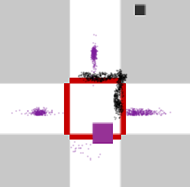
(a) GT

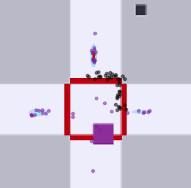
(b) WTA

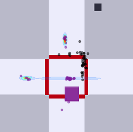
(c) RWTA

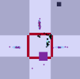
(d) EWTA

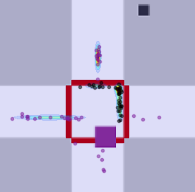
(e) DAC

Figure 4: The figure illustrates predicted hypotheses and learned mixture distribution of goals using different WTA objectives on the CPI test set. The purple and black box represent car and pedestrian at their current location. Predicted hypotheses are shown in their respective colours. (e) captures the data distribution better with hypothesis spread out across the crosswalk resembling the ground truth distribution of points.

We first evaluate our proposed Divide and Conquer technique on the synthetic Car Pedestrian dataset[34]. Further, we show evaluations of DAC and the proposed anchor based prediction technique on Nuscenes[5] prediction dataset.

5.1 Car Pedestrian Dataset

Unlike real world settings where only a single outcome is observed, CPI dataset consists of interacting agents with multi-modal ground truths. We aim to evaluate how well our multi-hypothesis predictions capture the true distribution of samples in the test set. We use a similar training strategy from [34] using a ResNet-18 [20] encoder backbone where we train a two-stage mixture density network [4]. The first stage takes past observations of the car and pedestrian as the inputs and predicts $k$ output hypotheses containing future goals of both actors after $\Delta t$ timestep. We train the first stage using different variants of the winner-takes-all loss function. The second stage then fits a mixture distribution with $M$ modes over the hypothesis by predicting soft-assignments for the outputs. We refer readers to Equations 7, 8 and 9 from [34] for more details about calculating the parameters for the mixture distribution. We use evaluation metrics such oracle error (FDE) and Earth Mover’s Distance (EMD) used in [34].

Oracle error (FDE) measures the diversity of our outputs predictions by choosing the closest hypothesis with the ground truth.

EMD distance quantifies the amount of probability mass that has to be moved from the predicted distribution to match the true distribution.

From Table 1 it can be inferred that the proposed DAC method outperforms the other variants of WTA objective showing that DAC captures the data distribution better compared to EWTA, RWTA and WTA. This can also been seen in Figure 4 where network trained with DAC objective captures the ground truth distribution of actors better compared to other variants. The average EMD of the proposed DAC is significantly better than WTA and comparable to EWTA and RWTA objective. DAC better captures goals for the cars that spread across compared to pedestrian goals. Moreover, as shown by Table 1, the average oracle error (FDE) for the DAC method is significantly lower compared to other variants confirming that DAC WTA produces diverse hypotheses.

Table 1: Comparion of Methods on CPI dataset based on FDE and EMD metrics, where p - pedestrian and c - car

Method	pFDE	cFDE	Avg FDE	pEMD	cEMD	Avg EMD
DAC	5.56	5.61	5.58	1.14	1.48	1.31
EWTA[34]	5.8	5.63	5.76	1.09	1.59	1.34
RWTA[39]	4.90	9.56	7.23	1.02	1.64	1.33
WTA[30]	5.32	6.32	5.82	1.17	2.41	1.79
CVAE	15.9	19.2	17.6	1.72	2.74	2.23

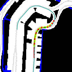
(a)

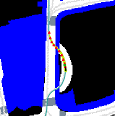
(b)

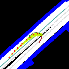
(c)

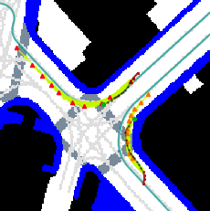
(d)

Figure 5: Shows example predictions from ALAN. The past trajectory is shown in brown and the GT is shown in black. The endpoint of GT is shown as a green dot. The input lane anchor is shown in cyan, with predicted trajectories in green and their endpoints as triangles. (a) and (b) shows predictions that follow a complex lane structure. Anchor based predictions can be beneficial especially for a longer prediction horizon as the complexity of the trajectory increases anchors can be helpful in following the semantics. (c) predicts a U-turn with appropriate dynamics when the lane of interest is in opposite direction and (d) shows a multi-agent prediction scenario.

Table 2: Nuscenes Trajectory Prediction Benchmark

Model	mADE_1	mADE_5	mADE_10	Miss_2_5	Miss_2_10	mFDE_1	mFDE_5	mFDE_10	OffRoadRate
cxx	-	1.63	1.29	69	60	8.86	-	-	0.08
pq	-	2.23	1.68	69	56	9.56	-	-	0.12
CoverNet[38]	-	2.62	1.92	76	64	11.36	-	-	0.13
MTP [12]	4.42	2.22	1.74	74	67	10.36	4.83	3.54	0.25
MultiPath [8]	4.43	1.78	1.55	78	76	10.16	3.62	2.93	0.36
Trajectron++[42]	-	1.88	1.51	70	57	9.52	-	-	0.25
MHA_JAM [36]	3.69	1.81	1.24	59	45	8.57	3.72	2.21	0.07
ALAN (top-M)	4.62	1.87	1.22	60	49	9.98	3.54	1.87	0.01
ALAN (Oracle)	4.61	1.78	1.16	59	48	9.95	3.29	1.70	0.01
ALAN (BofA)	4.67	1.77	1.10	57	45	10.0	3.32	1.66	0.01

Table 3: Ablation Study on Nuscenes dataset

Model	mADE_1	mADE_5	mADE_10	Miss_2_5	Miss_2_10	mFDE_1	mFDE_5	mFDE_10	OffRoadRate
CVAE	5.51	2.12	1.55	76	62	12.03	4.45	2.85	0.03
MCL + Global	8.45	2.85	1.88	87	75	17.52	5.34	3.05	0.16
MCL + Hyper	5.55	1.99	1.33	72	58	12.11	3.81	2.26	0.12
MCL + Poly	6.50	2.03	1.27	77	57	13.6	3.88	2.01	0.05
MCL + LA - $nt$	4.69	2.62	1.45	78	59	9.86	4.83	2.26	0.05
MCL + LA - $ntxy$	6.65	2.14	1.41	75	53	13.86	3.97	2.18	0.01
MCL + LA - $ntxy$ + Reg. + WTA	7.45	3.91	1.72	82	71	13.5	6.49	2.37	0.01
MCL + LA - $ntxy$ + Reg. + RWTA	4.41	2.55	1.21	64	45	9.22	5.03	1.77	0.01
MCL + LA - $ntxy$ + Reg. + EWTA	4.38	2.06	1.20	64	52	9.16	3.83	1.76	0.01
MCL + LA - $ntxy$ + Reg. + DAC	4.31	2.10	1.17	63	50	9.06	3.98	1.73	0.01

5.2 Nuscenes Dataset

Nuscenes[5] contains a large collection of complex road scenarios from cities of Boston and Singapore. Approximately 40k instances were extracted for the prediction dataset. It contains challenging sequences such as ones with U-turns and complex road layouts.

5.2.1 Baselines

We show comparisons of our ALAN predictions with several baseline methods evaluated on Nuscenes benchmark. MTP [12] uses rasterized image as input to predict trajectories. CoverNet [38] uses fixed set of trajectories to solve the prediction as a classification over the trajectory set. Multipath [8] is the closest baseline that uses time parameterized anchor trajectories obtained from the train set and formulates the problem as regression of offset values with respect to their anchor heads. MHA_JAM [36] is recent method that uses joint agent-map representation to produce outputs with multi-head attentions. Trajectron++ [42] is graph recurrent model that predicts trajectories incorporating agent dynamics and semantics. We utilize the numbers for [12] and [8] from [36].

5.2.2 Metrics

We use standard evaluation metrics such as Average Displacement Error (mADE_M) and Final Displacement Error (mFDE_M). Further, we compute miss rate (Miss_d,M) of top $M$ likely trajectories with the GT. A set of predictions is considered to be a miss if there’s no hypothesis across predictions having maximum displacement point less than the threshold $d$. OffRoadRate computes percentage of output trajectories that fall outside the drivable region. We use the example API provided by Nuscenes to compute our metrics.

5.2.3 Quantitative Results

We first show that ALAN can achieve on par or better performance compared to our baseline approaches. Here we evaluate ALAN with different anchor sampling strategies, top-M, oracle and best-of-all (BofA). In ALAN (top-M) we pick top $M$ trajectory outputs from different anchors based on predicted IOC scores for each trajectory. ALAN (oracle) uses oracle anchor with highest centerline score (see supplementary) and ALAN (BofA) picks best from top-k hypothesized lane anchors. Results represented by Table 2 demonstrate that all our ALAN evaluations either show on par performance or significantly outperform other baselines on several metrics with at least 11% improvements in terms of mADE₁₀ and 25% boost in terms mFDE₁₀ from our BofA method. Moreover, all our ALAN predictions provide an OffRoadRate of $0.01$ showing only 1% of the predicted trajectories fall outside the road. This is significantly lower compared to other baselines where they have 7% or higher OffRoadRate’s. This strong coupling of output predictions with the semantics can be attributed to the anchor lanes that help in providing output predictions in the lane direction. Other approaches like [8, 38] use trajectories extracted from the train set, either as anchors or to perform classification, this can lead to poor generalization of outputs to unseen scenarios and trajectories with complex lane structure. Moreover, we would like to note that our ALAN performance is understated due issues such as unconnected lanes and places without lane centerlines in the data leading to bad anchors. We talk about such situations in supplementary but have not removed these here for benchmark purposes.

Ablation Study:

Further, we perform ablation studies of our ALAN along with the proposed DAC and other variants in Table 3. We first introduce hypercolumn descriptors [2] to extract multi-scale features and compare it with using a global context vector fed as input to the decoder. Then we investigate several variants of our ALAN predictions. First, we add reference centerline as input and predict trajectories in $xy$ coordinate space (MCL + Poly). This improved the performance significantly. Using lane centerlines as anchors and predicting trajectories in $nt$ space (MCL+LA-$nt$) performed a little worse but we attribute this to networks difficulty in figuring out agent dynamics from anchor based inputs. For example, two trajectories with the same $nt$ coordinates can have different dynamics based on the lane that they’re travelling. So we further add $xy$ coordinates as input and predict auxiliary trajectories in cartesian space (MCL+LA-$ntxy$). As it is shown in Table 3, making such auxiliary predictions improved the primary anchor based outputs. Further, we regularize our anchor outputs using auxiliary predictions and vice-versa. The intuition is that anchor outputs can benefit from auxiliary predictions when there’s a bad input anchor since auxiliary predictions are not constrained to provide trajectories along the lane direction. Adding a regularizer to match our primary and auxiliary trajectories significantly improved our anchor output performance as seen in Table 3 from MCL+LA-$ntxy$+Reg values.

Comparing variations of ALAN in Table 3, it can be inferred that network trained with DAC beats the EWTA and RWTA objectives confirming the ability of the proposed DAC method to produce diverse hypotheses and capture the data distribution better. Please note that although we perform evaluations for DAC in trajectory prediction setting, MCL[30] techniques are applicable in a wide range of problems where our DAC method can be used as a better initialization strategy for WTA objectives.

5.2.4 Qualitative Results

Figure 5 shows qualitative results from ALAN. In general, using lane as anchors and transforming the prediction problem to $nt$ space can be helpful to guide the prediction and follow semantics. As we predict trajectories for a longer time horizon the executed trajectories become complex with more than just one straight or turn maneuvers where using lane as anchors can simplify the problem.

6 Conclusion

In this paper we addressed issues related to learning multi-modal outputs using WTA objectives and using driving knowledge to impose constraints on output predictions. First, we introduced a novel DAC approach that learns diverse hypotheses to capture the data distribution without any spurious modes. Further, we introduced ALAN that provides diverse and context aware trajectories using anchor lanes. Our experiments on both synthetic and real data demonstrated the superiority of our proposed DAC method in learning multi-modal outputs. In addition, we demonstrated that using lane anchors can be helpful in providing accurate predictions with strong semantic coupling.

1 Further Details for ALAN

1.1 Network Architecture

In this section, we provide more details about our network architecture.

Centerline Encoder:

It takes lane anchor for each individual agent in the form of $p\times 2$ points and reshapes them as $2p\times 1\times 1$ vector. We then pass it through a series of $1\times 1$ convolutions with 256,128,64 output filters.

Past Trajectory Encoder:

It contains an embedding layer and an LSTM encoder. The embedding layer takes a 5 dimensional vector containing $X_{i}^{t},N_{i,k}^{t}$ for every timestep along with a boolean mask indicating if trajectory information is available for the timestep and produces an embedded vector of 16 dimensions. Then the embedded past trajectory is fed through a LSTM of hidden size 64 to produce a past state vector of 64 dimensions.

Multi-Agent Convolutional Encoder:

The past state vector (64 dim) and embedded centerline vector (64 dim) are concatenated to form a 128 dimensional vector for every agent. The agent specific information is then encoded at its respective location to form a $H\times W\times 128$ vector. This along with the BEV map of size $H\times W\times 3$ is provided as input to this module. The module uses a ResNet-18[20] encoder backbone where we replace the first layer with a convolutions of $3\times 3$ kernel size and stride 2. We then pass the features through ResNet[20] base layers from 1 to 7.

Hypercolumn Trajectory Decoder:

First we extract hypercolumn descriptors for every agent based on the agent’s location in the BEV map. Specifically, we extract hypercolumn features from layers 0,2,4,5,6,7 and pass them through a series of $1\times 1$ convolutions containing 2048,1024,1024 filters. Finally, a $1\times 1$ output convolution then produces primary and auxiliary outputs.

Ranking Module:

It takes in 1024 features vectors from the Hypercolumn Trajectory Decoder before the final output layer and passes them through a $1\times 1$ convolution with 1024 filters and finally produces $M$ trajectory scores as output.

1.2 Learning

Our input BEV map is of size $256\times 256$ dimensions at a resolution of $0.5m$ per pixel. The models are trained with Adam[26] optimizer with an initial learning rate of 1e-4 and batch size 8. We use exponential lr decay with gamma value 0.95 called after every epoch. The hypotheses are split in case of DAC after every 2000 iterations and the models are trained for 150k iterations (approximately 38 epochs). The ALAN is implemented in pytorch[37] and trained on NVIDIA RTX 2080Ti GPU.

1.3 Nuscenes Dataset

Approximately 2.5% of validation set contains bad anchors, such as some due to either unconnected lanes or places without lane centerlines. In such cases, for the benchmark evaluation we use the nearest lane centerline that is closest to the trajectory. Further, we evaluate our method by approximately removing examples which have average normal distance of the past trajectory to nearest lane greater than a threshold distance (3 meters) and compare it with baselines [38, 12]. As seen from Table 1 our proposed ALAN provides even better performance when bad anchors are removed.

Table 1: Nuscenes Evaluations. Removing bad anchors based on normal distance to lane (threshold = 3m). Total validation examples after removing = 8823.

Model	mADE_1	mADE_5	mADE_10	Miss_2_5	Miss_2_10	mFDE_1	mFDE_5	mFDE_10	OffRoadRate
CoverNet[38]	6.81	3.09	2.39	87	76	13.9	5.92	4.27	0.13
MTP [12]	4.14	2.80	1.74	70	53	9.91	6.42	3.71	0.11
ALAN (top-M)	4.49	1.79	1.14	58	47	9.76	3.41	1.76	0.003
ALAN (Oracle)	4.48	1.70	1.08	57	46	9.72	3.16	1.60	0.004
ALAN (BofA)	4.54	1.69	1.03	55	43	9.84	3.20	1.56	0.006

2 Anchor Retrieval

Nuscenes[5] provides HD map data containing lane centerline information represented a sequence of points. We follow steps similar to [25] in order to retrieve plausible lanes.

Identify Closest Lanes Given a position of the vehicle in city coordinates we first identify a set of closest lane segments to the vehicle within a radius $d$.

Retrieve Candidate Anchors We identify plausible lane anchors by traversing through successor and predecessor lanes till a threshold distance. Several connected lane segments from an anchor.

Prune Duplicate Anchors We then filter candidate anchors by removing lanes, which are a subset of others.

Heuristic based Pruning Based on the vehicle’s velocity we identify a look ahead point on the lane for a future timestep $T$ and remove duplicate anchors which pass through the same point. This is done to further reduce the number of plausible anchors and remove duplicates which only diverge after a sufficient distance from the vehicle’s position.

Distance Along Lane Score Then we rank the candidates anchors based on distance travelled along the lane by the vehicle. First, we calculate the corresponding $nt$ coordinates for the trajectory along every plausible anchor. The score is determined as the absolute sum of normal values for every timestep in the trajectory. Anchors are then ranked based on their scores.

Centerline Yaw Score Further, we rank candidate anchors which have same distance along lane score based on centerline yaw score. It is calculated as the absolute difference between yaw angle of the vehicle and lane yaw angle at a point closest to the vehicle.

Learning Every plausible anchor divided into $p$ equally spaced points, in our case $p=150$. For training, we use the oracle anchor where oracle is determined based on the trajectory information from $1...T$. During inference, for ALAN (top-M) we rank trajectories using observed locations from $1...t_{obs}$.

3 Additional Results

In this section, we show some additional quantitative and qualitative comparisons for the proposed DAC and ALAN framework.

3.1 DAC Qualitative Comparisons

We evaluate our proposed DAC through additional simulations including modes with non-uniform probabilities and compare it with previous WTA objectives [30, 39, 34] (shown in Figure 1). As observed, WTA[30] leaves many hypothesis untrained. While RWTA[39] solves the convergence problem in WTA it brings non-winner hypothesis to an equilibrium position due to residual constraints. Further, EWTA[34] captures the data distribution better but still suffers from the problem of spurious modes as hypothesis can be attracted towards many ground truths and finally left untrained as only top k hypotheses are penalized. Finally, proposed DAC captures the data distribution as good or better even when modes have such low likelihoods and solves the problem of spurious modes by making use of all hypotheses. In every stage, DAC reaches close to a Centroidal Voronoi Tessellation[15] with effective number of outputs increasing at every stage, leading to hypotheses capturing some probability mass and thus avoiding the spurious mode problem.

3.2 DAC on Other Networks

Further, we implement our proposed DAC on other popular networks such as DeepLabV3[10] where we train and test on PascalVOC2012[16] dataset for semantic segmentation task and calculate the IoU scores for 21 classes. Our mIoU scores across all clases is reported in Table 2. Here, we modify the final layer of DeepLabV3[10] to contain multiple segmentation heads in order to implement DAC and WTA.

Method (mIoU)	DeepLabV3	DeepLabV3 + WTA	DeepLabV3 + DAC
Pascal2012 (val set)	76.83	82.14	83.44

Table 2: mIoU score for DeepLabV3[10] on Pascal2012[16] dataset with no multimodality, WTA(k=3) and DAC on Pascal[16] val set.

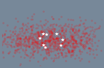
(a) Init

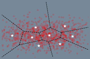
(b) WTA

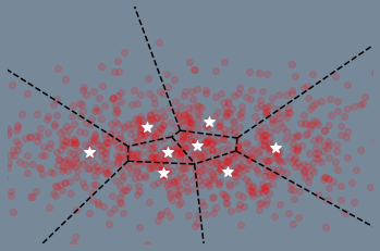
(c) RWTA

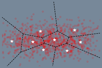
(d) EWTA

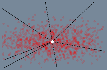
(e) DAC - Depth 1

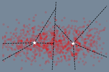
(f) DAC - Depth 2

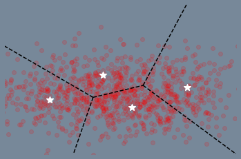
(g) DAC - Depth 3

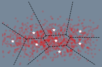
(h) DAC - Depth 4

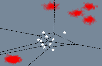
(i) Init

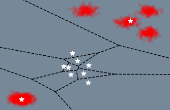
(j) WTA

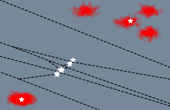
(k) RWTA

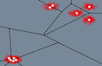
(l) EWTA

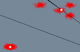
(m) DAC - Depth 2

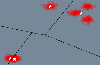
(n) DAC - Depth 3

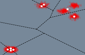
(o) DAC - Depth 4

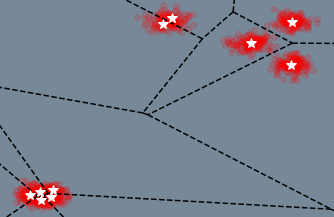
(p) DAC - Depth 5

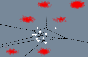
(q) Init

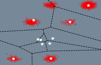
(r) WTA

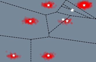
(s) RWTA

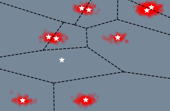
(t) EWTA

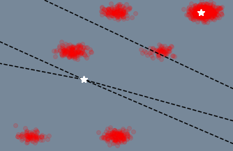
(u) DAC - Depth 2

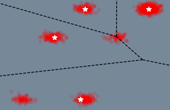
(v) DAC - Depth 3

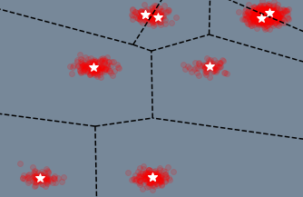
(w) DAC - Depth 4

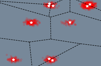
(x) DAC - Depth 5

Figure 1: Additional toy examples including modes with non-uniform likelihoods comparing DAC with other WTA family of objectives. The first two rows shows a mixture distribution with high variance and second two rows show a well separated gaussian mixture model. Other examples contain modes with $\pi=\{5,7.5,12.5,50\}\%$. As seen from Row 3, WTA captures the distribution poorly by either leaving many hypotheses untrained or by introducing spurious modes that do not correspond to the data distribution. On the other hand, every hypothesis in proposed DAC captures some part of the data as seen from its voronoi space.

3.3 ALAN Qualitative Comparisons

Figure 2 shows qualitative comparison of ALAN with other baselines [38, 12].

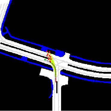
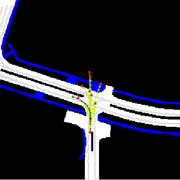
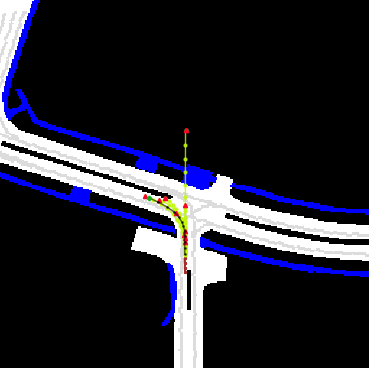
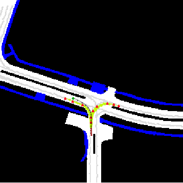
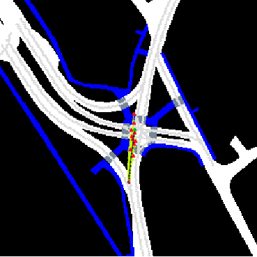
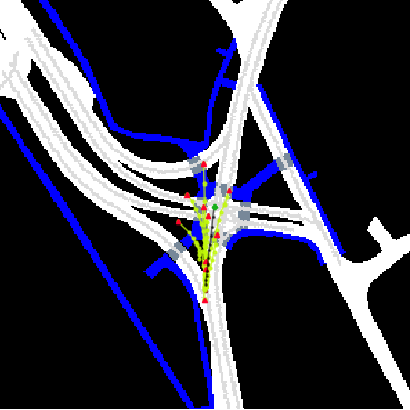
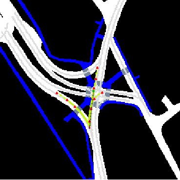
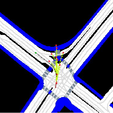
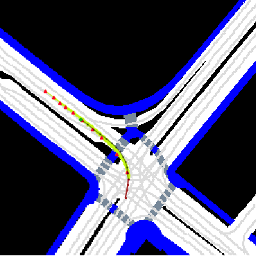
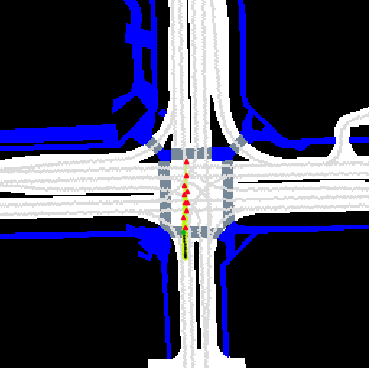
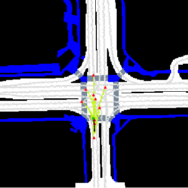
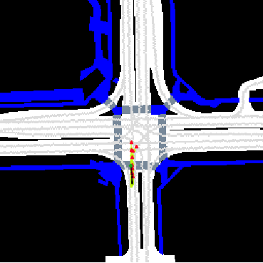
(a) MTP[12]

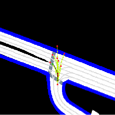
(b) CoverNet[38] Epsilon=8

(c) CoverNet[38] Epsilon=2

(d) ALAN (Ours)

Figure 2: Shows comparison of ALAN predictions with baselines. The past trajectory is in brown and the GT is shown in black. The endpoint of GT is shown as a green dot. The predicted trajectories are shown in green and their endpoints as triangles. The final trajectories are chosen based on the predicted IOC score of each trajectory. As observed ALAN predictions are more semantically aligned in comparison.

References

- [1] Alexandre Alahi, Kratarth Goel, Vignesh Ramanathan, Alexandre Robicquet, Li Fei-Fei, and Silvio Savarese. Social lstm: Human trajectory prediction in crowded spaces. In Proceedings of the IEEE conference on computer vision and pattern recognition, pages 961–971, 2016.
- [2] Aayush Bansal, Xinlei Chen, Bryan Russell, Abhinav Gupta, and Deva Ramanan. Pixelnet: Towards a general pixel-level architecture, 2016.
- [3] Apratim Bhattacharyya, Bernt Schiele, and Mario Fritz. Accurate and diverse sampling of sequences based on a “best of many” sample objective. In Proceedings of the IEEE Conference on Computer Vision and Pattern Recognition, pages 8485–8493, 2018.
- [4] C. Bishop. Mixture density networks. 1994.
- [5] Holger Caesar, Varun Bankiti, Alex H. Lang, Sourabh Vora, Venice Erin Liong, Qiang Xu, Anush Krishnan, Yu Pan, Giancarlo Baldan, and Oscar Beijbom. nuscenes: A multimodal dataset for autonomous driving. arXiv preprint arXiv:1903.11027, 2019.
- [6] Sergio Casas, Cole Gulino, Simon Suo, Katie Luo, Renjie Liao, and Raquel Urtasun. Implicit latent variable model for scene-consistent motion forecasting. In Proceedings of the European Conference on Computer Vision (ECCV). Springer, 2020.
- [7] Sergio Casas, Cole Gulino, Simon Suo, and Raquel Urtasun. The importance of prior knowledge in precise multimodal prediction, 2020.
- [8] Yuning Chai, Benjamin Sapp, Mayank Bansal, and Dragomir Anguelov. Multipath: Multiple probabilistic anchor trajectory hypotheses for behavior prediction. arXiv preprint arXiv:1910.05449, 2019.
- [9] Ming-Fang Chang, John Lambert, Patsorn Sangkloy, Jagjeet Singh, Slawomir Bak, Andrew Hartnett, De Wang, Peter Carr, Simon Lucey, Deva Ramanan, et al. Argoverse: 3d tracking and forecasting with rich maps. In Proceedings of the IEEE Conference on Computer Vision and Pattern Recognition, pages 8748–8757, 2019.
- [10] Liang-Chieh Chen, George Papandreou, Florian Schroff, and Hartwig Adam. Rethinking atrous convolution for semantic image segmentation, 2017.
- [11] Qifeng Chen and Vladlen Koltun. Photographic image synthesis with cascaded refinement networks, 2017.
- [12] Henggang Cui, Vladan Radosavljevic, Fang-Chieh Chou, Tsung-Han Lin, Thi Nguyen, Tzu-Kuo Huang, Jeff Schneider, and Nemanja Djuric. Multimodal trajectory predictions for autonomous driving using deep convolutional networks. 2019 International Conference on Robotics and Automation (ICRA), May 2019.
- [13] Debadeepta Dey, Varun Ramakrishna, Martial Hebert, and J Andrew Bagnell. Predicting multiple structured visual interpretations. In Proceedings of the IEEE International Conference on Computer Vision, pages 2947–2955, 2015.
- [14] Nemanja Djuric, Vladan Radosavljevic, Henggang Cui, Thi Nguyen, Fang-Chieh Chou, Tsung-Han Lin, and Jeff Schneider. Motion prediction of traffic actors for autonomous driving using deep convolutional networks. arXiv preprint arXiv:1808.05819, 2, 2018.
- [15] Qiang Du, Vance Faber, and Max Gunzburger. Centroidal voronoi tessellations: Applications and algorithms. SIAM review, 41(4):637–676, 1999.
- [16] M. Everingham, L. Van Gool, C. K. I. Williams, J. Winn, and A. Zisserman. The PASCAL Visual Object Classes Challenge 2012 (VOC2012) Results. http://www.pascal-network.org/challenges/VOC/voc2012/workshop/index.html.
- [17] Jiyang Gao, Chen Sun, Hang Zhao, Yi Shen, Dragomir Anguelov, Congcong Li, and Cordelia Schmid. Vectornet: Encoding hd maps and agent dynamics from vectorized representation. In Proceedings of the IEEE/CVF Conference on Computer Vision and Pattern Recognition, pages 11525–11533, 2020.
- [18] Agrim Gupta, Justin Johnson, Li Fei-Fei, Silvio Savarese, and Alexandre Alahi. Social gan: Socially acceptable trajectories with generative adversarial networks. In Proceedings of the IEEE Conference on Computer Vision and Pattern Recognition, pages 2255–2264, 2018.
- [19] Abner Guzman-Rivera, Dhruv Batra, and Pushmeet Kohli. Multiple choice learning: Learning to produce multiple structured outputs. In Advances in Neural Information Processing Systems, pages 1799–1807, 2012.
- [20] Kaiming He, Xiangyu Zhang, Shaoqing Ren, and Jian Sun. Deep residual learning for image recognition, 2015.
- [21] Sepp Hochreiter and Jürgen Schmidhuber. Long short-term memory. Neural Comput., 9(8):1735–1780, Nov. 1997.
- [22] Joey Hong, Benjamin Sapp, and James Philbin. Rules of the road: Predicting driving behavior with a convolutional model of semantic interactions. In Proceedings of the IEEE Conference on Computer Vision and Pattern Recognition, pages 8454–8462, 2019.
- [23] Xin Huang, Stephen G. McGill, Jonathan A. DeCastro, Luke Fletcher, John J. Leonard, Brian C. Williams, and Guy Rosman. Diversitygan: Diversity-aware vehicle motion prediction via latent semantic sampling, 2020.
- [24] Boris Ivanovic and Marco Pavone. The trajectron: Probabilistic multi-agent trajectory modeling with dynamic spatiotemporal graphs, 2018.
- [25] Siddhesh Khandelwal, William Qi, Jagjeet Singh, Andrew Hartnett, and Deva Ramanan. What-if motion prediction for autonomous driving, 2020.
- [26] Diederik P. Kingma and Jimmy Ba. Adam: A method for stochastic optimization, 2017.
- [27] Kris M Kitani, Brian D Ziebart, James Andrew Bagnell, and Martial Hebert. Activity forecasting. In European Conference on Computer Vision, pages 201–214. Springer, 2012.
- [28] Vineet Kosaraju, Amir Sadeghian, Roberto Martín-Martín, Ian Reid, Hamid Rezatofighi, and Silvio Savarese. Social-bigat: Multimodal trajectory forecasting using bicycle-gan and graph attention networks. In Advances in Neural Information Processing Systems, pages 137–146, 2019.
- [29] Namhoon Lee, Wongun Choi, Paul Vernaza, Christopher B. Choy, Philip H. S. Torr, and Manmohan Krishna Chandraker. Desire: Distant future prediction in dynamic scenes with interacting agents. 2017 IEEE Conference on Computer Vision and Pattern Recognition (CVPR), pages 2165–2174, 2017.
- [30] Stefan Lee, Senthil Purushwalkam, Michael Cogswell, Viresh Ranjan, David Crandall, and Dhruv Batra. Stochastic multiple choice learning for training diverse deep ensembles, 2016.
- [31] Stéphanie Lefèvre, Christian Laugier, and Javier Ibañez-Guzmán. Exploiting map information for driver intention estimation at road intersections. In 2011 IEEE Intelligent Vehicles Symposium (IV), pages 583–588. IEEE, 2011.
- [32] Ming Liang, Bin Yang, Rui Hu, Yun Chen, Renjie Liao, Song Feng, and Raquel Urtasun. Learning lane graph representations for motion forecasting. arXiv preprint arXiv:2007.13732, 2020.
- [33] Wenjie Luo, Bin Yang, and Raquel Urtasun. Fast and furious: Real time end-to-end 3d detection, tracking and motion forecasting with a single convolutional net. In Proceedings of the IEEE conference on Computer Vision and Pattern Recognition, pages 3569–3577, 2018.
- [34] Osama Makansi, Eddy Ilg, Ozgun Cicek, and Thomas Brox. Overcoming limitations of mixture density networks: A sampling and fitting framework for multimodal future prediction. 2019 IEEE/CVF Conference on Computer Vision and Pattern Recognition (CVPR), Jun 2019.
- [35] Francesco Marchetti, Federico Becattini, Lorenzo Seidenari, and Alberto Del Bimbo. Mantra: Memory augmented networks for multiple trajectory prediction. In Proceedings of the IEEE/CVF Conference on Computer Vision and Pattern Recognition, pages 7143–7152, 2020.
- [36] Kaouther Messaoud, Nachiket Deo, Mohan M. Trivedi, and Fawzi Nashashibi. Trajectory prediction for autonomous driving based on multi-head attention with joint agent-map representation, 2020.
- [37] Adam Paszke, Sam Gross, Francisco Massa, Adam Lerer, James Bradbury, Gregory Chanan, Trevor Killeen, Zeming Lin, Natalia Gimelshein, Luca Antiga, Alban Desmaison, Andreas Kopf, Edward Yang, Zachary DeVito, Martin Raison, Alykhan Tejani, Sasank Chilamkurthy, Benoit Steiner, Lu Fang, Junjie Bai, and Soumith Chintala. Pytorch: An imperative style, high-performance deep learning library. In H. Wallach, H. Larochelle, A. Beygelzimer, F. d'Alché-Buc, E. Fox, and R. Garnett, editors, Advances in Neural Information Processing Systems 32, pages 8024–8035. Curran Associates, Inc., 2019.
- [38] Tung Phan-Minh, Elena Corina Grigore, Freddy A. Boulton, Oscar Beijbom, and Eric M. Wolff. Covernet: Multimodal behavior prediction using trajectory sets. In Proceedings of the IEEE/CVF Conference on Computer Vision and Pattern Recognition (CVPR), June 2020.
- [39] Christian Rupprecht, Iro Laina, Robert DiPietro, Maximilian Baust, Federico Tombari, Nassir Navab, and Gregory D. Hager. Learning in an uncertain world: Representing ambiguity through multiple hypotheses, 2017.
- [40] Amir Sadeghian, Vineet Kosaraju, Ali Sadeghian, Noriaki Hirose, Hamid Rezatofighi, and Silvio Savarese. Sophie: An attentive gan for predicting paths compliant to social and physical constraints. In Proceedings of the IEEE Conference on Computer Vision and Pattern Recognition, pages 1349–1358, 2019.
- [41] Amir Sadeghian, Ferdinand Legros, Maxime Voisin, Ricky Vesel, Alexandre Alahi, and Silvio Savarese. Car-net: Clairvoyant attentive recurrent network. In Proceedings of the European Conference on Computer Vision (ECCV), pages 151–167, 2018.
- [42] Tim Salzmann, Boris Ivanovic, Punarjay Chakravarty, and Marco Pavone. Trajectron++: Dynamically-feasible trajectory forecasting with heterogeneous data, 2020.
- [43] Shashank Srikanth, Junaid Ahmed Ansari, Karnik Ram R, Sarthak Sharma, Krishna Murthy J., and Madhava Krishna K. Infer: Intermediate representations for future prediction, 2019.
- [44] NN Sriram, Buyu Liu, Francesco Pittaluga, and Manmohan Chandraker. Smart: Simultaneous multi-agent recurrent trajectory prediction. In European Conference on Computer Vision, 2020.
- [45] N. N. Sriram, G. Kumar, A. Singh, M. S. Karthik, S. Saurav, B. Bhowrnick, and K. M. Krishna. A hierarchical network for diverse trajectory proposals. In 2019 IEEE Intelligent Vehicles Symposium (IV), pages 689–694, 2019.
- [46] Richard S Sutton and Andrew G Barto. Reinforcement learning: An introduction. MIT press, 2018.
- [47] Jur Van Den Berg, Stephen J Guy, Ming Lin, and Dinesh Manocha. Reciprocal n-body collision avoidance. In Robotics research, pages 3–19. Springer, 2011.
- [48] Ye Yuan and Kris Kitani. Diverse trajectory forecasting with determinantal point processes, 2019.
- [49] Wenyuan Zeng, Shenlong Wang, Renjie Liao, Yun Chen, Bin Yang, and Raquel Urtasun. Dsdnet: Deep structured self-driving network. arXiv preprint arXiv:2008.06041, 2020.
- [50] Hang Zhao, Jiyang Gao, Tian Lan, Chen Sun, Benjamin Sapp, Balakrishnan Varadarajan, Yue Shen, Yi Shen, Yuning Chai, Cordelia Schmid, et al. Tnt: Target-driven trajectory prediction. arXiv preprint arXiv:2008.08294, 2020.
- [51] Tianyang Zhao, Yifei Xu, Mathew Monfort, Wongun Choi, Chris Baker, Yibiao Zhao, Yizhou Wang, and Ying Nian Wu. Multi-agent tensor fusion for contextual trajectory prediction. In Proceedings of the IEEE Conference on Computer Vision and Pattern Recognition, pages 12126–12134, 2019.
Supplementary Material