The scaling limit of the longest increasing subsequence

Abstract

We provide a framework for proving convergence to the directed landscape, the central object in the Kardar-Parisi-Zhang universality class. For last passage models, we show that compact convergence to the Airy line ensemble implies convergence to the Airy sheet. In i.i.d. environments, we show that Airy sheet convergence implies convergence of distances and geodesics to their counterparts in the directed landscape. Our results imply convergence of classical last passage models and interacting particle systems. Our framework is built on the notion of a directed metric, a generalization of metrics which behaves better under limits.

As a consequence of our results, we present a solution to an old problem: the scaled longest increasing subsequence in a uniform permutation converges to the directed geodesic.

1 Introduction

1.1 Random plane geometry

The goal of this paper is to set up a framework for proving convergence of random directed plane geometry models to a universal limit, the directed landscape.

In these models, we have a random “distance” function $d$ defined on the plane or a periodic subset, such as a lattice. A simple example is the model on the front page, which is equivalent to the Seppäläinen-Johansson model, see Example 1.2. For this picture, each horizontal edge in $\mathbb{Z}^{2}$ is given an i.i.d. length $1$ or $2$ and all vertical edges have length $1$.

In such models, how far should a point $p$ be from the origin for $d(0,p)$ have standard deviation roughly $\sigma$? The empirical answer is order $\sigma^{3}$, and histograms of $d(0,p)$ show that the distribution is not normal. This suggests that the noise in the random plane geometry has a nontrivial structure.

To understand this structure, it helps to consider a simpler deterministic setting. In Euclidean geometry, paths from $0$ to a point at distance $\sigma^{3}$ from $0$ whose length is $\sigma^{3}+\sigma$ deviate from a straight line by distance $O(\sigma^{2})$. This suggest that the noise in our random metric has nontrivial correlations in a scaling window of size $\sigma^{3}$ in the main direction and $\sigma^{2}$ in the transversal direction. To make this more explicit, given a direction $v_{0}$, there are vectors $v||v_{0}$ and $u$ and a scalar $\mu$ so that as $\sigma\to\infty$ we expect

$$d(\sigma^{2}ux+\sigma^{3}vs,\sigma^{2}uy+\sigma^{3}vt)=(t-s)\sigma^{3}\mu-\sigma\mathcal{L}(x,s;y,t)+o(\sigma).$$ (1.1)

Here $\mathcal{L}$ is a limiting universal random plane geometry called the directed landscape, constructed in Dauvergne, Ortmann and Virág (2018). The negative sign in front of $\sigma$ in (1.1) is a convention.

In Dauvergne, Ortmann and Virág (2018), it was shown that one particular random metric model – Brownian last passage percolation – converges to the directed landscape. This paper can be though of as a followup. We give a brief summary of the new results.

1.2 New results

We develop a general framework for the convergence of last passage models to the directed landscape, and apply this framework to several classical models. The following main contributions are described in more detail in the later part of the introduction.

• We develop the notion of directed metric spaces, of which usual metrics, last passage percolation models, and the directed landscape are all examples. We formalize the notion of geodesics and establish hypograph and graph topologies for studying convergence.

• As a result of this framework, convergence of geodesics will follow from convergence of the corresponding directed metric spaces in either topology.

• We introduce a maximal inequality for last passage percolation that allows for simple tightness conditions in the hypograph topology. For tightness in the stronger graph topology and for stronger exponential tightness, we give a general chaining argument that will apply to all models.

• We use the RSK isometry to prove that convergence to the Airy sheet for last passage models follows from convergence to the Airy line ensemble without any additional assumptions. For i.i.d. lattice last passage models, convergence to the Airy line ensemble also implies convergence to the directed landscape and convergence of geodesics.

• We use our framework to prove convergence to the directed landscape for geometric and exponential last passage percolation (this part of the present work is used in Busani et al. (2022) and Ganguly and Zhang (2022)), Poisson last passage percolation across lines and in the plane (used in Dauvergne (2022)).

• We prove that coupled taseps started from multiple initial conditions converges to KPZ fixed points coupled via the directed landscape. To do so, we give a general framework for moving from convergence of directed metrics to convergence of metric interfaces. Tasep height functions are interfaces in the exponential last passage metric. This part of the present work has been used in Rahman and Virág (2021) to show convergence of second class particle trajectories.

• We give a new definition for the Airy sheet in terms of the Airy line ensemble, resolving Conjecture 14.1 from Dauvergne, Ortmann and Virág (2018).

• We establish new symmetries for the Airy sheet and the Airy line ensemble.

• We prove that the shape of the longest increasing subsequence in a random permutation converges to the directed geodesic.

1.3 Directed metric spaces

We expect $\mathcal{L}$ to be the limit of most random metrics in the plane built out of independent noise. However, $\mathcal{L}$ itself is not a metric, and neither are the last passage models that are the main focus of this paper. Because of this, we need a generalized notion of metrics.

A directed metric of positive sign on a set $S$ is a function $d:S^{2}\to\mathbb{R}\cup\{\infty\}$ satisfying

$$d(p,p) =0,\qquad\qquad p\in S,$$

$$d(p,q)+d(q,r) \geq d(p,r),\qquad p,q,r\in S.$$

Unlike with ordinary metrics, directed metrics can be asymmetric and may take negative values. We say that $d$ is a directed metric of negative sign if $-d$ is a directed metric of positive sign.

All ordinary metrics are directed metrics of positive sign. A familiar example of a directed metric of negative sign is the $L^{p}$-norm on $\mathbb{R}^{d}$ for $p\in(0,1)$: set $\|x\|_{p}^{p}=\sum x_{i}^{p}$ when all $x_{i}\geq 0$ and $-\infty$ otherwise, and let $d(x,y)=\|x-y\|_{p}$.

The notion of a directed metric unifies the usual notions of metric, distance in directed graphs, and last passage percolation. In addition, directed metrics are closed under the deterministic shifts used in the approximation (1.1), while ordinary metrics are not. Properties of directed metrics are studied in Section 5.

1.3.1 Classical models and other examples

The following are selected examples from Section 6. Most of these are integrable classical models whose fine scaling behaviour is accessible. To construct these examples, we introduce the useful notion of an induced metric. In the positive sign setting, given a function $d_{0}:A\to\mathbb{R}\cup\{\infty\}$ for some subset $A\subset S^{2}$, the induced metric of positive sign is the supremum of all directed metrics on $S$ with $d|_{A}\leq d_{0}$, see Definition 5.3. Induced metrics of negative sign are defined the same way, with the inequality reversed and supremum replaced by infimum.

Example 1.1.

Let $G$ be an undirected graph, and let $d_{0}(x,y)=1$ whenever $(x,y)$ is an edge. The metric of positive sign on $G$ induced by $d_{0}$ is the usual graph distance.

This generalizes to weighted, directed graphs: when $d_{0}$ is defined on all directed edges to be the edge weight, the induced metric is the weighted directed graph distance.

Example 1.2 (Seppäläinen-Johansson).

Continuing Example 1.1, let $G$ be the square lattice $\mathbb{Z}^{2}$ where $(x,y)$ is a directed edge whenever $y$ is directly north or directly east of $x$. Let $d_{0}=0$ on all north edges, and let $d_{0}$ be $0$ or $1$ on east edges according to independent coin tosses with probability $p$. The resulting induced metric of positive sign on $\mathbb{Z}^{2}$ is a random directed metric known as the Seppäläinen-Johansson model with parameter $p$, see Figure 1. This model was introduced by Seppäläinen (1998) and further studied by Johansson (2001).

Example 1.3 (Geometric and exponential last passage).

Let $G=(V,E)$ be a directed graph, and define $d_{0}((x,y),(y,z))=1$ for any pair of directed edges $(x,y),(y,z)$. The induced metric $d$ on $E$ of negative sign assigns to each pair $e,f$ of directed edges the length of the longest walk starting with $e$ and ending with $f$, as measured by the number of intermediate vertices.

If we set $d_{0}((x,y),(y,z))=w(y)$ for all directed edges for some weight function $w$ on $V$, the induced metric corresponds to last passage percolation.

When $G=\mathbb{Z}^{2}$ with edges directed north or east as in Example 1.2, and the weights $w(y)$ are i.i.d. and nonnegative, we call the corresponding model i.i.d. lattice last passage percolation. This model is integrable when the weights $w(y)$ are exponential or geometric. Throughout the paper, we assume all exponential random variables are mean $1$, and that geometric random variables have mean $\gamma\in(0,\infty)$ and are supported on $\{0,1,2,\dots\}$.

This distance function can be extended to be defined on $V\cup E$ rather than just on $E$. This is done by instead looking at the metric induced by the function given by $d_{0}((x,y),y)=w(y)$ and $d_{0}(x,(x,y))=0$, see Example 6.2.

For studying Examples 1.2 and 1.3, our labelling of the points in $\mathbb{Z}^{2}$ will be as in Figure 1, where indices increase as we move south and east. There are natural reasons for making this unusual choice that are related to the combinatorics of last passage percolation, see Section 2.

Figure 1: An instance of the Seppäläinen-Johansson model. The solid edges have weight $1$ and the dashed edges have weight $0$. The path of red vertices is a geodesic from $(1,3)$ to $(5,1)$.

Example 1.4 (Poisson last passage).

Let $P\subset\mathbb{R}^{2}$ be a discrete set of points, and for $a,c\in\mathbb{R}^{2}$ with $a_{1}\leq c_{1},a_{2}\leq c_{2}$, let

$$d_{0}(a,c)={\mathbf{1}}\Big{\{}[a_{1},c_{1}]\times[a_{2},c_{2}]\mbox{ contains a point of $P$ different from }a\Big{\}}.$$

When $P$ is Poisson point process, the induced metric of negative sign on $\mathbb{R}^{2}$ is Poisson last passage percolation, see Definition 13.5.

Example 1.5 (Semidiscrete metrics, Poisson lines, Brownian last passage percolation).

Let $f_{i}:\mathbb{R}\to\mathbb{R},i\in\mathbb{Z}$ be a sequence of cadlag functions with no negative jumps. For $(x,m),(y,n)\in\mathbb{R}\times\mathbb{Z}$, let

$$d_{0}((x,m),(y,n))=\begin{cases}f_{m}(y)-f_{m}(x^{-}),\qquad&m=n,x<y\\ f_{n}(x)-f_{n}(x^{-})\qquad&m=n+1,x=y\end{cases}$$

We call the directed metric of negative sign on $\mathbb{R}\times\mathbb{Z}$ induced by $d_{0}$ the semidiscrete metric of $f$.

When the $f_{i}$ are independent Brownian motions, the semidiscrete metric of negative sign is Brownian last passage percolation, see Section 13.1.4. When the $f_{i}$ are independent Poisson counting processes, the semidiscrete metric is called last passage percolation across Poisson lines, see Section 13.1.3. It is equivalent to the Hammersley process on the lattice, see Seppäläinen (1996) Section 3.1, and Ferrari and Martin (2006).

All examples introduced so far can alternately be described by optimizing over paths. For example, in the setting of Example 1.5, let $x\leq y$ and $n\geq m$. A path $\pi$ from $(x,n)$ to $(y,m)$ is a union of closed intervals

$$[t_{i},t_{i-1}]\times\{i\}\subset\mathbb{R}\times\mathbb{Z},\qquad i=m,m+1,\ldots,n,\qquad x=t_{n}\leq t_{n-1}\leq\cdots\leq t_{m}\leq t_{m-1}=y.$$

The length of $\pi$ is given by

$$|\pi|_{f}=\sum_{i=m}^{n}f_{i}(t_{i-1})-f_{i}(t_{i}^{-}).$$ (1.2)

Geodesics in these models are paths that maximize length among paths between the same endpoints. When $f_{m}$ is continuous at $x$, then $d((x,m),(y,n))$ is the maximal path length.

Example 1.6.

The directed landscape $\mathcal{L}$ is a random directed metric of negative sign on $\mathbb{R}^{2}$. It is continuous on the parameter space

$$\mathbb{R}^{4}_{\uparrow}=\{(x,s;y,t)\in\mathbb{R}^{4}:s<t\},$$

and satisfies $\mathcal{L}(u;v)=-\infty$ for all $(u;v)\notin\mathbb{R}^{4}_{\uparrow}$ with $u\neq v$. Because of this, we can think of $\mathcal{L}$ as a spacetime metric, which only assigns finite distances to points in the right time order. Paths and geodesics in $\mathcal{L}$ only move forward in time, and between any pair of points $(p,q)\in\mathbb{R}^{4}_{\uparrow}$, there is a almost surely a unique $pq$-geodesic in $\mathcal{L}$. The directed landscape is independent on disjoint time strips $\mathbb{R}\times[s_{1},t_{1}],\dots,\mathbb{R}\times[s_{2},t_{2}]$ and has natural scale and translation invariance properties. See Definition 6.6 and surrounding discussion for more detail.

1.4 The main theorem for classical models

In the classical integrable last passage models above (Examples 1.2, 1.3, 1.4, and Poisson lines and Brownian last passage percolation in Example 1.5), we can establish convergence to the directed landscape. The following table gives scaling parameters, which are built from a direction $\rho\in(0,\infty)$. For the geometric distribution with mean $\gamma$, set $\bar{\gamma}=\sqrt{\gamma(\gamma+1)}$. For the Seppäläinen-Johansson model with Bernoulli-$p$ variables, we set $\lambda=p/(1-p)$, and additionally assume that $\rho>1/\lambda$.

$$\begin{array}[]{l|cc|ccc}&\|(x,-y)\|_{d}&\chi^{3}&\alpha&\beta&\chi/\tau^{2}\\ \hline\cr\text{S-J}&\frac{(\sqrt{x\lambda}-\sqrt{y})^{2}}{\lambda+1}&-\frac{\sqrt{\lambda}(\sqrt{\lambda\rho}-1)^{2}(\sqrt{\rho}+\sqrt{\lambda})^{2}}{\sqrt{\rho}(\lambda+1)^{3}}&\frac{(\sqrt{\rho\lambda}-1)^{2}}{\lambda+1}&\frac{\lambda-\sqrt{\lambda/\rho}}{\lambda+1}&\frac{-\sqrt{\lambda}}{4(\lambda+1)\rho^{3/2}}\\ \text{Geometric}&(x+y)\gamma+2\sqrt{xy}\bar{\gamma}&\frac{\bar{\gamma}\left(\bar{\gamma}(1+\rho)+(2\gamma+1)\sqrt{\rho}\right)^{2}}{\sqrt{\rho}}&\gamma(\rho+1)+2\bar{\gamma}\sqrt{\rho}&\gamma+\frac{\bar{\gamma}}{\sqrt{\rho}}&\frac{\bar{\gamma}}{4\rho^{3/2}}\\ \text{Exponential }&(\sqrt{x}+\sqrt{y})^{2}&\frac{\left(\sqrt{\rho}+1\right)^{4}}{\sqrt{\rho}}&(\sqrt{\rho}+1)^{2}&1+\frac{1}{\sqrt{\rho}}&\frac{1}{4\rho^{3/2}}\\ \text{Poisson}&\|(x,y)\|_{d}=2\sqrt{xy}&\sqrt{\rho}&2\sqrt{\rho}&\frac{1}{\sqrt{\rho}}&\frac{1}{4\rho^{3/2}}\\ \text{Brownian}&2\sqrt{xy}&\rho^{3/2}&2\sqrt{\rho}&\frac{1}{\sqrt{\rho}}&\frac{1}{4\rho^{3/2}}\\ \text{Poisson lines}&x+2\sqrt{xy}&\sqrt{\rho}(1+\sqrt{\rho})^{2}&\rho+2\sqrt{\rho}&1+\frac{1}{\sqrt{\rho}}&\frac{1}{4\rho^{3/2}}\\ \end{array}$$

The table above uniquely determines the scaling parameters $\chi,\alpha,\beta$ and $\tau>0$. The value $\chi$ is positive for all models except the Seppäläinen-Johansson model, the only directed metric of positive sign in the table.

Theorem 1.7.

Given $\rho$, consider either geometric, exponential, or Brownian last passage percolation with $\chi,\tau,\alpha,\beta$ in the table above. Let $v=(\rho,-1),u=(\tau,0)$. Then for any sequence of $\sigma\to\infty$, there is a coupling of identically distributed copies $d_{\sigma}$ of $d$ and the directed landscape $\mathcal{L}$ so that

$$d_{\sigma}(x\sigma^{2}u+s\sigma^{3}v,y\sigma^{2}u+t\sigma^{3}v)=\alpha\sigma^{3}(t-s)+\beta\tau\sigma^{2}(y-x)+\chi\sigma(\mathcal{L}+o_{\sigma})(x,s;y,t),$$ (1.3)

where the random function $o_{\sigma}$ is small in the sense that for any compact set $K\subset\mathbb{R}^{4}_{\uparrow}$, $\sup_{K}|o_{\sigma}|\to 0$ a.s. and there is $c>0$ so that with $\mathfrak{l},\mathfrak{r}$ as in the table below,

$$\mathbb{E}\exp\Big{(}c\sup_{K}(o_{\sigma}^{-})^{\mathfrak{l}}+(o_{\sigma}^{+})^{\mathfrak{r}}\Big{)}\to 1.$$ (1.4)

The same result holds for Poisson last passage, with $v=(\rho,1)$ instead of $(\rho,-1)$. For the Seppäläinen-Johansson model and the Poisson line model, the result also holds except the convergence of $o_{\sigma}\to 0$ is in the weaker hypograph topology, see Sections 1.9.1, 13.1.3 and 13.1.6 for details.

$$\begin{array}[]{l|c|c}&\text{Left tail exponent }\mathfrak{l}&\text{Right tail exponent }\mathfrak{r}\\ \hline\cr\text{Geometric}&3&1\\ \text{Exponential }&3&1\\ \text{Poisson}&3&3/2\\ \text{Brownian}&3/4&3/2\end{array}$$

For the five discrete or semi-discrete models above, note that we need to modify the arguments of $d_{\sigma}$ in (1.3) to ensure that they lie in the appropriate discrete set, see Section 13 for details. On the almost sure set where convergence holds in Theorem 1.7, we have the following strong convergence of geodesics.

Theorem 1.8.

Let $\pi_{\sigma}$ be the image of an arbitrary geodesic in $d_{\sigma}$ under the linear map satisfying $\sigma^{3}v\mapsto(0,1)$ and $\sigma^{2}u\mapsto(1,0)$. Assume that as $\sigma\to\infty$, the endpoints of $\pi_{\sigma}$ converge to points $p,q$ with $(p,q)\in\mathbb{R}^{4}_{\uparrow}$.

Then $\pi_{\sigma}$ is precompact in the Hausdorff topology, and on the almost sure set where there is a unique $pq$-geodesic $\pi$ in $\mathcal{L}$, $\pi_{\sigma}\to\pi$. In the four cases in Theorem 10.3 where $o_{\sigma}\to 0$ compactly on $\mathbb{R}^{4}_{\uparrow}$, all subsequential limits of $\pi_{\sigma}$ are $pq$-geodesics in $\mathcal{L}$ even if there are multiple $pq$-geodesics.

In Theorem 1.8 and in the sequel, we say that a sequence of functions $f_{n}\to f$ compactly if $f_{n}\to f$ uniformly on compact sets. Compact convergence of $o_{\sigma}$ is a consequence of (1.4). In the context of Brownian last passage percolation, slightly weaker versions of Theorem 1.7 and Theorem 1.8 were shown in Dauvergne, Ortmann and Virág (2018). We have included the results here for completeness. Theorems 1.7 and 1.8 are proven in Section 13.

In many models, the main direction $v$ in the above scaling can change with $\sigma$ arbitrarily, and we can still conclude hypograph convergence to the directed landscape and convergence of geodesics. See Section 13 for the corresponding theorems.

Remark 1.9 (Scaling heuristics).

As $\sigma\to\infty$, $d(\sigma^{3}p,\sigma^{3}q)/\sigma^{3}\to\|p-q\|_{d}$. The function $\|\cdot\|_{d}:\mathbb{R}^{2}\mapsto\mathbb{R}\cup\{\infty\}$ ($-\infty$ if the metric $d$ is of negative sign) is a directed norm: it satisfies the triangle inequality, $\|0\|_{d}=0$ and $\|av\|_{d}=a\|v\|_{d}$ for $a>0$. The parameters $\beta,\alpha$ and $\chi/\tau^{2}$ are determined by the Taylor expansion of the norm near $v$ in the first coordinate direction:

$$\|v+(x,0)\|_{d}=\alpha+\beta x-\frac{\chi}{\tau^{2}}x^{2}+o(x^{2}).$$ (1.5)

The magnitude of $\chi$ is given by the standard deviation

$$\operatorname{SD}d(0,\sigma^{3}v)/\sigma\to|\chi|\,\operatorname{SD}\mathcal{L}(0,0;0,1),$$

where $\mathcal{L}(0,0;0,1)$ has GUE Tracy-Widom law. The sign of $\chi$ is the opposite of the sign of the directed metric $d$.

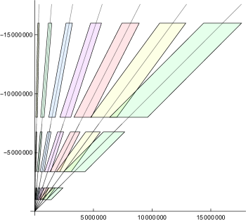
Figure 2: Scaling windows for geometric last passage percolation with mean $\gamma=1$ at slopes $\rho=(i/7)^{2}$, $i=1\ldots 7$ and $\sigma=100,200,300$.

Remark 1.10 (Choice of direction).

Our choice of $u=(\tau,0)$ as the multiple of the first coordinate vector is convenient for the proof, but we can set $u=\tau e$ for any vector $e$ linearly independent from $v$. The Taylor expansion of $\|v+xe\|_{d}$ determines the new parameters $\beta,\chi^{2}/\tau$ as in (1.5), while $\alpha,\chi$ are unchanged. When $e=(0,1)$, the space direction is vertical, rather than horizontal. When $e$ is a tangent vector to the $\|\!\cdot\!\|_{d}$-disk of radius $\|v\|_{d}$ at $v$, then $\beta=0$, and simpler asymptotics equivalent to (1.1) hold.

More generally, let $v=(v_{1},\pm v_{2})$ where $v_{1},v_{2}>0$ and $\pm$ is negative except in the case of Poisson last passage. Let $u=(u_{1},u_{2})$, linearly independent from $v$. Then by a straightforward change-of-variables argument, Theorem 1.7 holds as follows:

$$d_{\sigma}(x\sigma^{2}u+s\sigma^{3}v,y\sigma^{2}u+t\sigma^{3}v)=\tilde{\alpha}\sigma^{3}(t-s)+\tilde{\gamma}\sigma^{2}(y-x)+\tilde{\chi}\sigma(\mathcal{L}+o_{\sigma})(x,\tilde{\omega}s;y,\tilde{\omega}t),$$ (1.6)

where $\alpha,\beta,\chi,\tau$ are from the table and

$$\tilde{\alpha}=v_{2}\alpha,\quad\tilde{\eta}=\frac{u_{1}+(v_{1}/v_{2})u_{2}}{\tau},\quad\tilde{\gamma}=\beta\tilde{\eta}\tau-\alpha u_{2},\quad\tilde{\chi}=\chi\tilde{\eta}^{1/2},\quad\tilde{\omega}=v_{2}/\tilde{\eta}^{3/2}.$$

Remark 1.11 (Possible projects).

Some of the results above can be improved. The Brownian left tail exponent $3/4$ is not optimal. This is because the directed metric takes negative values, and so more care is needed in the chaining argument, see Section 11. For the Poisson lines and Seppäläinen-Johansson models, tail bounds are needed to get the stronger version of convergence. This could be done in two ways: (i) analysis of the contour integral formulas, (ii) by a combinatorial connection to other models where tail bounds are known.

1.5 Outline of the proof

Theorem 1.7 is proven in three steps. First the results are shown with the initial location $(x,s)=0$ and the final time $t=1$ fixed. This part of the analysis is well-known, and in the present generality it is shown in the companion paper Dauvergne, Nica and Virág (2019). To go further, we will use the RSK correspondence, for which we need to understand distances along multiple disjoint paths, as explained below. This will allow us to prove Theorem 1.7 when we only fix $s=0$ and $t=1$, and let $x,y$ vary. The corresponding process $\mathcal{S}(x,y)$ is called the Airy sheet, first defined in Dauvergne, Ortmann and Virág (2018).

The directed landscape is assembled from compositions of independent Airy sheets as an inverse limit, analogously to Lévy’s construction of Brownian motion. The corresponding convergence statements are proven this way. Extra work is needed to prove tightness in sufficiently strong topologies.

1.6 RSK

The key ingredient for all our proofs is a ‘Greene’s theorem formulation’ of the classical Robinson-Schensted-Knuth correspondence (RSK). In this paper we use a version of this correspondence, introduced in Dauvergne, Nica and Virág (2021), that unites classical RSK, dual RSK and continuous path RSK. We will also be able to take limits without leaving this universe.

Let $\mathcal{D}^{n}_{0}$ be the space of $n$-tuples of cadlag functions from $[0,\infty)\to\mathbb{R}$ without negative jumps. For continuous $f\in\mathcal{D}^{n}_{0}$, recalling the notion of path length from (1.2), we can define

$$f[(x,m)^{k}\to(y,n)^{k}]=\sup\sum_{i=1}^{k}|\pi_{i}|_{f},$$

where the supremum is over all sets of $k$ paths $\pi_{1},\dots,\pi_{k}$ from $(x,m)$ to $(y,n)$ that are disjoint away from $x$ and $y$. The same definition works for general $f\in\mathcal{D}^{n}_{0}$ but with a few extra technicalities, see Section 2.2 for details. In our setting the RSK transform maps a function $f\in\mathcal{D}^{n}_{0}$ to its melon $Wf$ as follows.

Definition 1.12.

Let $f[p^{0}\to q^{0}]=0$, and for $k\geq 1$, set $f[p\to_{\Delta k}q]=f[p^{k}\to q^{k}]-f[p^{k-1}\to q^{k-1}]$. The RSK or melon map $W:\mathcal{D}^{n}_{0}\to\mathcal{D}^{n}_{0}$ is defined by

$$Wf_{k}(y)=f[(0,n)\to_{\Delta k}(y,1)].$$

The RSK map has two remarkable properties. First, it is an isometry.

Theorem 1.13 (RSK isometry).

For all $0\leq x\leq y$,

$$f[(x,n)\to(y,1)]=Wf[(x,n)\to(y,1)].$$ (1.7)

Second, because the RSK map $W$ is (one marginal of) a bijection, certain nice measures on $\mathcal{D}^{n}_{0}$ have tractable pushforwards under $W$. For example, independent Brownian motions get mapped to nonintersecting Brownian motions under $W$, see Theorem $7$ in O’Connell and Yor (2002). Such properties make RSK a perfect tool for the probabilistic analysis of directed geometry problems.

In particular, we may hope to understand limits of random directed metrics in the plane by taking the limits of the RSK isometry (1.7). This project was carried out for Brownian last passage percolation in Dauvergne, Ortmann and Virág (2018). One goal of this paper is to make it applicable in a more general setting.

1.7 The scaling limit of melons and the Airy sheet

In integrable settings, the melon side of the RSK isometry is an ensemble of nonintersecting random walks. The natural limit of nonintersecting random walks is an infinite sequence of nonintersecting Brownian motions known as the parabolic Airy line ensemble. This object was first described by Prähofer and Spohn (2002) as the scaling limit of the polynuclear growth model, and realized as a system of nonintersecting locally Brownian functions by Corwin and Hammond (2014). The parabolic Airy line ensemble is a random sequence of functions $\mathfrak{A}=\{\mathfrak{A}_{1}>\mathfrak{A}_{2}>\ldots\}$. The process $\mathcal{A}(x)=\mathfrak{A}(x)+x^{2}$ is stationary in $x$, and on every finite interval each $\mathfrak{A}_{i}$ is absolutely continuous with respect to Brownian motion.

In the companion paper Dauvergne, Nica and Virág (2019) it was shown that in many models, the limit of the melon is the parabolic Airy line ensemble. One of the main theorems of the present paper is that convergence to the Airy line ensemble implies convergence of the melon side of the RSK isometry (1.7) to a last passage problem in $\mathfrak{A}$. The resulting process characterizes the Airy sheet, see Definition 1.22 and Figure 3 for more details.

Figure 3: The Airy sheet $\mathcal{S}(x,y)$ function plot and contour plot. The ridge corresponds to $x=y$. See the decay $\mathcal{S}(x,x+y)\sim-y^{2}$.

1.8 General convergence to the Airy sheet

Theorem 1.14.

For each $n$, let $F_{n}$ be a sequence of $n$ random cadlag functions as in Example 1.5. Let $a_{n}\leq 0$, $c_{n}\in\mathbb{R}$. If for every $z\in\mathbb{R}$, the sequences of random functions

$$F_{n}[(z+a_{n},n)\to_{\Delta k}(z+\cdot,1)]+c_{n},\quad\;\text{and}\;\quad F_{n}[(z+a_{n}-\cdot,n)\to_{\Delta k}(z,1)]+c_{n}$$

converge in law in the product of Skorokhod topologies to the parabolic Airy line ensemble, then in some coupling of the processes $F_{n}$ and an Airy sheet $\mathcal{S}$ we have

$$F_{n}[(x+a_{n},n)\to(y,1)]+c_{n}\to\mathcal{S}(x,y)\qquad\mbox{compactly a.s.}$$

Theorem 1.14 is an immediate consequence of Theorem 4.4. A key ingredient in the proof of this theorem is tightness for convergence to the Airy sheet $\mathcal{S}$. This follows from tightness of the single-variable marginals, and the fact that both $\mathcal{S}$ and its prelimits share a useful property: they are cumulative distribution functions of the corresponding shock measures, random measures on $\mathbb{R}^{2}$. See Section 4 for details.

1.9 From two times to all times to geodesics

Convergence to the Airy sheet requires no additional assumptions beyond Skorokhod convergence to the Airy line ensemble.

The directed landscape $\mathcal{L}$ is defined from independent Airy sheets analogously to how Brownian motion is defined from independent normal distributions, see Definition 6.6 for more details.

Because of this, in many i.i.d models convergence to the Airy sheet immediately implies a weak type of finite-dimensional distribution convergence that we refer to as multi-time convergence. This level of convergence does not imply a strong notion of convergence of geodesics, so in Section 7 we consider two stronger topologies. In Sections 10 and 11 we give sufficient conditions for tightness in these topologies.

The first topology is essentially compact convergence. Since compact convergence is not a separable topology on discontinuous functions, and our prelimits are often discontinuous, we replace it by a graph convergence in the localized Hausdorff metric. This convergence requires an extra moment assumption, but it implies a very strong form of convergence of geodesics.

A weaker topology is that of hypograph convergence. Translated to the language of functions, a sequence $f_{n}$ converges to a continuous function $f$ in this topology if $(f_{n}-f)^{+}\to 0$ uniformly on compact sets, and if for every $x$ we can find a sequence $x_{n}\to x$ such that $f_{n}(x_{n})\to f(x)$, see Section 7 for more precise statements. This topology has the advantage that for i.i.d. models, we need no extra assumptions in addition to Airy sheet convergence. It also implies a fairly strong form of geodesic convergence, but it allows for ‘holes’ in the prelimit that geodesics tend to avoid. Graph convergence ensures that such holes do not exist, while the hypograph topology ignores them.

We give an example of a sequence of last passage models satisfying multi-time convergence but not hypograph convergence at the beginning of Section 10, and an example satisfying multi-time and hypograph convergence but not graph convergence in Example 13.13.

1.9.1 Hypograph convergence

The key ingredient for proving hypograph convergence is a last passage version of Doob’s classical maximal inequality. It is proven in the setting of semidiscrete metrics of negative sign applied to sequences of independent functions with independent increments, see Example 1.5. Lattice last passage models can be embedded as semidiscrete metrics, and hence also fit into this setting.

Theorem 1.15.

Let $A,B\subset\mathbb{R}\times\mathbb{Z}$ be finite unions of bounded product sets. For $p,q\in\mathbb{R}\times\mathbb{Z},c\in\mathbb{R}$ and $\epsilon>0$ we have

$$\;\mathbb{P}\left(d(p,q)\leq c-2\epsilon,c<d(A,B)\right)\leq\;\sup_{a\in A}\mathbb{P}(d(p,a)<-\epsilon)+\sup_{b\in B}\mathbb{P}\left(d(b,q)<-\epsilon\right).$$ (1.8)

The maximal inequality is proven as Lemma 10.6. The version in that lemma is slightly stronger than Theorem 1.15 but more technical. Theorem 1.15 reduces hypograph convergence for models satisfying Airy sheet convergence to a simple one-dimensional convergence requirement called mobile Tracy-Widom convergence. This requirement is easy to check in all cases we study. For this theorem, let $d_{n}$ be a sequence of rescaled i.i.d. lattice last passage models, see Example 1.3. Extend these models to $\mathbb{R}^{4}_{\uparrow}$ using floors.

Theorem 1.16.

We have $d_{n}\stackrel{{\scriptstyle d}}{{\to}}\mathcal{L}$ in the hypograph topology provided that:

• (Mobile Tracy-Widom convergence) For any sequence $u_{n}\to u\in\mathbb{R}^{4}_{\uparrow}$, we have $d_{n}(u_{n})\stackrel{{\scriptstyle d}}{{\to}}\mathcal{L}(u).$

• (Airy sheet convergence) For all $s<t\in\mathbb{R}$ we have $d_{n}(\cdot,s;\cdot,t)\stackrel{{\scriptstyle d}}{{\to}}\mathcal{L}(\cdot,s;\cdot,t)$ in the graph topology.

See Theorem 10.3 for a stronger version and Section 10 for more precision about the scaling assumptions on $d_{n}$. Hypograph convergence deterministically implies convergence of geodesics, see Theorems 8.5 and 8.7. In particular, Theorem 8.7 implies that if $d_{n}\to\mathcal{L}$ almost surely in the hypograph topology and $u_{n}\to u\in\mathbb{R}^{4}_{\uparrow}$, then on the almost sure set where there is a unique $u$-geodesic $\pi$ in $\mathcal{L}$, any sequence of $u_{n}$-geodesics converges to $\pi$ in the Hausdorff topology.

1.9.2 Compact convergence

Graph convergence is a separable substitute to compact convergence. It is equivalent to compact convergence when the limit is continuous, as is the case in our setting.

We show this type of convergence in the context of i.i.d. lattice last passage environments, Example 1.3. Let $d_{n}$ be a sequence of such environments rescaled so that $d_{n}\stackrel{{\scriptstyle d}}{{\to}}\mathcal{L}$ in the multi-time sense. In this setting, we have the following theorem.

Theorem 1.17.

Let $U=\{(0,0;0,x):-3\leq x\leq 3\}$. If for some $\delta>0$,

$$\limsup_{n\to\infty}\,\sup_{u\in U}\mathbb{E}\left(d_{n}(u)^{-}\right)^{5+\delta}<\infty,$$ (1.9)

then in some coupling $d_{n}\to\mathcal{L}$ compactly on $\mathbb{R}^{4}_{\uparrow}$.

Theorem 1.17 follows from Theorem 12.2, see Remark 12.3. Refer also to that theorem for precise details about the scaling of $d_{n}$. Theorem 1.17 shows that $5+\delta$ moments are sufficient for compact convergence. This is optimal; in Example 13.13 we give an example satisfying all the conditions of Theorem 1.17 but with $\delta=0$ where compact convergence fails.

Again, compact convergence deterministically implies convergence of geodesics. The type of convergence is stronger than in the hypograph setting. Indeed, Theorem 8.5 shows that if $u_{n}\to u\in\mathbb{R}^{4}_{\uparrow}$ and $d_{n}(u_{n})\to\mathcal{L}(u)$ then any sequence of $u_{n}$-geodesics in $d_{n}$ is precompact in the Hausdorff topology, and all subsequential limits are $u$-geodesics in $\mathcal{L}$.

One important advantage of compact convergence is that we get Airy sheet limits in all transversal directions. For last passage percolation across rectangles, this typically means that in a suitable scaling, convergence of left-to-right last passage values to the Airy sheet also implies convergence of bottom-to-top last passage values to the Airy sheet.

1.10 The longest increasing subsequence

Ulam (1961) asked what the length $L_{n}$ of the longest increasing subsequence in a uniform random $n$-element permutation is. Hammersley (1972) initiated the study of this problem in earnest, relating this length to a last passage value and established the asymptotics $L_{n}\sim c\sqrt{n}$. Vershik and Kerov (1977) and Logan and Shepp (1977) independently determined the value $c=2$, and Baik, Deift and Johansson (1999) identified the limiting fluctuations as the Tracy-Widom random variable $\mathcal{L}(0,0;0,1)$. Our main theorem concerns the shape of the sequence.

To state this theorem, recall from Example 1.6 that there is almost surely a unique geodesic in the directed landscape from $(0,0)$ to $(0,1)$. This geodesic is of the form $\{(\Pi(t),t):t\in[0,1]\}$ where $\Pi:[0,1]\to\mathbb{R}$ is a continuous function, Figure 4.

Figure 4: The directed geodesic, the scaling limit of the longest increasing subsequence.

Theorem 1.18.

Let $I_{n}$ be a longest increasing subsequence in a uniform random permutation of $\{1,\ldots,n\}$. We think of $I_{n}$ as a function from $\{1,\ldots,L_{n}\}\to\{1,\ldots,n\}$, and set $I_{n}(i)=n$ for $i>L_{n}$. Then in some coupling of the $I_{n}$ and $\mathcal{L}$,

$$I_{n}(\lfloor 2t\sqrt{n}\rfloor)=nt+2n^{5/6}\Pi(t)+n^{5/6}\epsilon_{n}(t),$$

where the error $\epsilon_{n}\to 0$ uniformly almost surely on $[0,1]$.

Note that since $L_{n}=2\sqrt{n}+O(n^{1/6})$, we could alternately replace the $\lfloor 2t\sqrt{n}\rfloor$ in the argument of $I_{n}$ above by ${\left\lfloor L_{n}t\right\rfloor}$. Theorem 1.18 is proven as part of Theorem 14.3 in Section 14.2. In that section we also show that two distinct longest increasing subsequences converge to the same geodesic, and also establish a Kolmogorov-Smirnov test for longest increasing subsequences in i.i.d. sampling: the limit is the directed geodesic, rather than a Brownian bridge. These theorems are all consequences of convergence of geodesics in Poisson last passage percolation, Theorem 1.8.

1.11 The limit of tasep

For the classical height function representation, let $\mathcal{H}$ be the set of functions $h:\mathbb{Z}\mapsto\mathbb{Z}$ so that $h(0)$ is even, and $|h(i)-h(i-1)|=1$ for all $i$. Continuous-time tasep $h_{t},t\in[0,\infty)$ is a Markov process on $\mathcal{H}$ in which each local maximum decreases by $2$ independently at rate 1.

There are several natural couplings of tasep in which all initial conditions are driven by a same noise. In each, the evolution can be interpreted as a discrete Hamilton-Jacobi equation in a noisy environment. Next, we construct the scaling limit of one of these couplings.

Let $X$ be an array of independent, mean $1$ exponential random variables indexed by even lattice points, i.e. $x\in\mathbb{Z}^{2}$ with $x_{1}+x_{2}\in 2\mathbb{Z}$. For any initial condition $h_{0}$, we can define a tasep evolution $h_{t}$ started from $h_{0}$ by letting $X(\kappa,x)$ be the increment between the first time that $h$ has a local maximum of value $\kappa$ at location $x$ (if this ever happens) and the time when $h(x)$ decreases to $\kappa-2$. The evolution of tasep from any initial condition given $X$ is deterministic. We show that in the scaling of functions $(\iota_{n}f)(x)=h(2n^{2/3}x)/n^{1/3}$, the limit of coupled tasep is contained in the directed landscape.

The corresponding limit theorem for a single tasep was shown by Matetski, Quastel and Remenik (2016), Theorem 3.13. We start by stating their theorem, reformulated in our language based on Nica, Quastel and Remenik (2020) and Dauvergne, Ortmann and Virág (2018).

Theorem 1.19 (Matetski, Quastel and Remenik (2016)).

Let $T\subset(0,\infty)$ be finite or countable. Let $h_{0}:\mathbb{R}\to\mathbb{R}\cup\{-\infty\}$, $h_{0}\not\equiv-\infty$ be fixed. There is a coupling of copies $X_{n}$ of $X$ and a directed landscape $\mathcal{L}$ so that on an event of probability $1$ for all $t\in T$ the following holds.

For any deterministic sequence of functions $h_{n,0}\in\mathcal{H}$ the tasep evolution $h_{n,t}$ satisfies

$$\iota_{n}(h_{n,2nt}+nt)(y)\to\sup_{x\in\mathbb{R}}h_{0}(x)+\mathcal{L}(x,0;y,t)$$ (1.10)

uniformly on compact subsets of $y\in\mathbb{R}$ as long as

• $\iota_{n}h_{n,0}\to h_{0}$, in the hypograph topology (see Section 7).

• there exists $s,a\in\mathbb{R}$ such that for all $n$ large enough, $\iota_{n}h_{n,0}(x)<a+s|x|$ for all $x$.

While this theorem is about the Markov process of height functions, our strengthening is about the driving noise of the discrete Hamilton-Jacobi equation.

Theorem 1.20 (Scaling limit of coupled tasep).

In the setting of Theorem 1.19, there is a coupling of $X_{n},X$ such that almost surely, (1.10) holds simultaneously for all $h_{n,0},h_{0}$ satisfying the bullet points.

In the discrete setting tasep is the evolution of the boundary of a growing disk in exponential last passage percolation. In the scaling limit, disk boundaries become straight lines, and the shapes of disks become second order effects, captured in the optimization problem (1.10). This phenomenon of interfaces is explored in Section 15. In Section 16, we use this interface machinery to translate convergence results about exponential last passage percolation into Theorem 1.20. Section 16 also contains a few other tasep convergence results, and a discussion of discrete-time tasep.

1.12 The Airy sheet conjecture

Convergence of symmetric lattice models to the Airy sheet can be used to extend the natural coupling between the Airy sheet and the Airy line ensemble used in the proof of Theorem 1.14, see Definition 3.3. In particular, we affirm Conjecture 14.1 in Dauvergne, Ortmann and Virág (2018) and show the following.

Theorem 1.21.

The Airy sheet is an explicit deterministic function of the Airy line ensemble.

More precisely, the following construction is equivalent to Definition 3.3.

Definition 1.22.

Let $\mathfrak{A}$ be a parabolic Airy line ensemble, and let $\mathfrak{A}^{*}(x)=\mathfrak{A}(-x).$ For $(x,y,z)\in\mathbb{Q}^{+}\times\mathbb{Q}^{2}$ let $x_{k}=(-\sqrt{k/(2x)},k)$ and let

$$\begin{split}\mathcal{S}^{\prime}(x,y,z)&=\mathfrak{A}[x_{k}\to(y,1)]-\mathfrak{A}[x_{k}\to(z,1)],\\ \mathcal{S}^{\prime}(-x,y,z)&=\mathfrak{A}^{*}[x_{k}\to(-y,1)]-\mathfrak{A}^{*}[x_{k}\to(-z,1)],\end{split}$$

for all large $k$, as the right hand sides stabilize when $k\to\infty$. For $(x,y)\in\mathbb{Q}\setminus\{0\}\times\mathbb{Q}$, define

$$\mathcal{S}(x,y)=\mathbb{E}\mathfrak{A}_{1}(0)+\lim_{n\to\infty}\frac{1}{2n}\sum_{z=-n}^{n}\mathcal{S}^{\prime}(x,y,z)-(z-x)^{2}.$$

The Airy sheet is the unique continuous extension of $\mathcal{S}$ to $\mathbb{R}^{2}$.

Theorem 1.21 is proven in Section 14.1.

1.13 Symmetries of the directed landscape

Some symmetries of the directed landscape were not shown in Dauvergne, Ortmann and Virág (2018) because the corresponding symmetries were not present in the prelimit. We rectify this in Section 14.1.

Proposition 1.23.

As a function of $x,s,y,$ and $t$, the directed landscape $\mathcal{L}$ satisfies

$$\mathcal{L}(x,s;y,t)\stackrel{{\scriptstyle d}}{{=}}\mathcal{L}(-x,s;-y,t)\stackrel{{\scriptstyle d}}{{=}}\mathcal{L}(y,-t;x,-s).$$

1.14 More related work

While the full construction of the directed landscape is quite recent, several aspects of it and of related KPZ models have been studied previously. We give a partial literature review here, focusing on the works most relevant to the current paper that are not discussed earlier in the introduction. For a gentle introduction suitable for a newcomer to the area, see Romik (2015). Review articles and books focusing on more recent developments include Corwin (2016); Ferrari and Spohn (2010); Quastel (2011); Weiss, Ferrari and Spohn (2017); Zygouras (2018).

Marginals of the directed landscape have been studied using exact formulas, including the works of Baik, Deift and Johansson (1999), Prähofer and Spohn (2002), and Matetski, Quastel and Remenik (2016) discussed above. In addition to these, Johansson and Rahman (2019) and Liu (2019) independently found formulas for the joint distribution of $\{\mathcal{L}(p,q_{i}):i\in\{1,\dots,k\}\}$, building on work of Johansson (2017, 2018) and Baik and Liu (2019).

These papers provide a strong integrable framework for understanding $\mathcal{L}$ and other KPZ models. There has also been a large amount of research investigating probabilistic and geometric properties of these models. For example, prior to Dauvergne, Ortmann and Virág (2018), tightness and regularity estimates for the directed landscape were obtained by Hammond and Sarkar (2018), Hammond (2017b), Pimentel (2018). Corwin, Quastel and Remenik (2015) also gave geometric heuristics predicting many properties of the directed landscape.

On of the most important probabilistic contributions to this area is the work of Corwin and Hammond (2014), which shows that the parabolic Airy line ensemble satisfies a certain Gibbs resampling property. We used this property in Dauvergne and Virág (2018) to further understand the parabolic Airy line ensemble, and in Dauvergne, Ortmann and Virág (2018) used this understanding to build the Airy sheet. The works of Hammond (2016, 2017b, 2017c), Calvert, Hammond and Hegde (2019) further refine the understanding of the Airy line ensemble using the Gibbs property.

Since the paper Dauvergne, Ortmann and Virág (2018) was posted, there has also been significant activity both on understanding the directed landscape itself and on using the directed landscape to better understand the KPZ fixed point. Bates, Ganguly and Hammond (2019) investigated the structure of exceptional points with multiple $\mathcal{L}$-geodesics, building on work of Hammond (2017a) and Basu, Ganguly and Hammond (2021), and Dauvergne, Sarkar and Virág (2020) showed that $\mathcal{L}$-geodesics have a deterministic three-halves variation.

The construction of the Airy sheet in terms of the Airy line ensemble has been used by Sarkar and Virág (2020) to prove Brownian absolute continuity of the KPZ fixed point, by Ganguly and Hegde (2021) to show that the difference profile in the Airy sheet is related to Brownian local time, and the prelimiting version has been used by Corwin, Hammond, Hegde and Matetski (2021) to study exceptional times in the KPZ fixed point. An extension of this construction has also been developed by Dauvergne and Zhang (2021) to study disjoint optimizers in $\mathcal{L}$ and build a theory of multi-point last passage values in the limit.

While this paper focuses on understanding limits of random metrics, positive temperature versions of these objects known as random polymers should also converge to the directed landscape. As with random metrics, a small collection of random planar polymer models have an integrable structure related to the geometric RSK correspondence, e.g. see O’Connell and Yor (2001), Seppäläinen (2012). Limits of these models yield the continuum random polymer, which is related to the KPZ equation via a Feynman-Kac formula, see Alberts et al. (2014). While the integrable structure of random polymer models is not as tractable as that of last passage models, Virág (2020) and Quastel and Sarkar (2020) both recently showed convergence in the random polymer setting to the full KPZ fixed point. Combining these results with the Gibbs ensemble characterization theorem in Dimitrov and Matetski (2021) and tightness results from Corwin and Hammond (2016), Dimitrov and Wu (2021) gives Airy line ensemble convergence for these models. Since Airy line ensemble convergence is essentially the only integrable ingredient we use in this paper, directed landscape convergence for these models should be within reach.

1.15 A short guide to the paper

There is admittedly a lot to unpack in the paper, so here is a short guide to orient the reader. Much of this is also discussed earlier in the introduction.

Sections 2-4 cover convergence to the Airy sheet. Of these, Sections 2 and 3 are brief and preliminary, and Section 4 contains the novel ideas and proofs. This part of the paper is essentially independent from the remaining sections.

The bulk of the paper’s new ideas are in Sections 5-11. Section 5 builds a theory of general directed metrics and their geodesics, Section 6 elaborates on the examples described earlier and gives precise ways to embed last passage metrics into $\mathbb{R}^{2}$, and Section 7 introduces the topologies we use in the paper. The next three sections give conditions for directed metrics to converge to the directed landscape in the sense of multi-time convergence (Section 9), in the hypograph topology (Section 10), and in the graph topology (Section 11).

Sections 12-14 apply the general theory built up that point. Section 12 ”puts everything together” for i.i.d. lattice last passage models. The proofs in this section are routine. Two results of interest in this section are Theorem 12.2 and Corollary 12.4, which make precise the idea that for an i.i.d. lattice last passage model, convergence to the Airy line ensemble implies convergence to the directed landscape. Section 13 gives a long-form list of precise theorems for all integrable models, elaborating on the theorems in Section 1.4. Treat this section as a dictionary. Section 14 proves the consequences of our main theorems: Theorems 1.18 and 1.21 and Proposition 1.23.

The final two sections consider random growth models that can be associated to last passage models. As discussed in Section 1.11, these two processes are connected by thinking of growth models as interfaces in directed metrics. Section 15 builds up a general theory of interface convergence for planar directed metrics, and Section 16 applies this theory to tasep.

2 Preliminaries: percolation across cadlag functions

In this section we introduce last passage percolation across cadlag functions. Cadlag last passage percolation is a common generalization of lattice last passage percolation with nonnegative weights and line models of last passage percolation. The Airy line ensemble appears as the common limit of all these models, and also fits within the cadlag framework. Basic combinatorial results about last passage percolation and the RSK correspondence have analogues in the cadlag setting. We use these results as the starting point for this paper.

A thorough treatment of cadlag last passage percolation is given in Dauvergne, Nica and Virág (2021). In that paper, basic combinatorial and probabilistic properties of cadlag RSK (e.g. isometry, bijectivity, measure preservation) are shown from first principles using the framework of Pitman transforms.

2.1 Last passage percolation across cadlag functions

A function from $f$ from an interval $I\subset\mathbb{R}$ to $\mathbb{R}$ is cadlag if $f(y)\to f(x)$ as $y\downarrow x$ in $I$, and the limit as $y\uparrow x$ also exists. This left-sided limit is denoted $f(x^{-})$. When $f(x^{-})\neq f(x)$, we say that $f(x)-f(x^{-})$ is a jump of $f$ and that $x$ is a jump location. Let $\mathcal{D}^{\mathbb{Z}}$ be the space of all functions

$$f:\mathbb{R}\times\mathbb{Z}\to\mathbb{R},\qquad(x,i)\mapsto f_{i}(x),$$

where each $f_{i}$ is a cadlag function whose jumps are all positive. We will often think of $f$ as a sequence of functions $(f_{i}:i\in\mathbb{Z})$ and we will refer to $f$ as an environment.

For $(p,q)=(x,n;y,m)\in(\mathbb{R}\times\mathbb{Z})^{2}$, we write $p\nearrow q$ if $x\leq y$ and $n\geq m$. This directionality is with respect to the coordinates used in Figure 5, where the line index is increasing as we go down the page. For $p\nearrow q$, a path $\pi$ from $p$ to $q$ is a union of closed intervals

$$[t_{i},t_{i-1}]\times\{i\}\subset\mathbb{R}\times I,\qquad i=m,m+1,\ldots,n,$$ (2.1)

where

$$x=t_{n}\leq t_{n-1}\leq\cdots\leq t_{m}\leq t_{m-1}=y.$$ (2.2)

The points $t_{i}$ are called the jump times of $\pi$. For two paths $\pi$ and $\rho$, we say that $\pi$ is to the left of $\rho$ if for every $(x,\ell)\in\pi$ there exists $(y,m)\in\rho$ such that $\ell\leq m$ and $x\leq y$. Equivalently, we say that $\rho$ is to the right of $\pi$. We say that $\pi$ and $\rho$ are essentially disjoint if the set $\pi\cap\rho$ is finite. See Figure 5 for an illustration of these definitions.

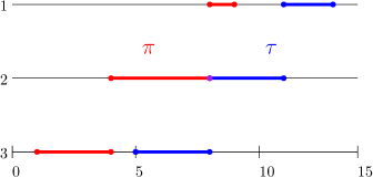
Figure 5: Cadlag paths: here $\pi$ is a path from $(1,3)$ to $(9,1)$ with jump times at $1,4,8,$ and $9$. The path $\pi$ is to the left of $\tau$ and is essentially disjoint from $\tau$, in spite of the single point of overlap at $(8,2)$.

For an environment $f\in\mathcal{D}^{\mathbb{Z}}$ and a path $\pi$, define the length of $\pi$ with respect to $f$ by

$$|\pi|_{f}=\sum_{i=m}^{n}f_{i}(t_{i-1})-f_{i}(t_{i}^{-}).$$

Informally, this definition is chosen so that the all jumps of $f$ that lie along the path $\pi$ are collected. An equivalent definition of path length is given through the finitely additive signed measure $df$ on $\mathbb{R}\times\mathbb{Z}$. Define

$$df\left([x,y]\times\{i\}\right)=f_{i}(y)-f_{i}(x^{-}).$$

Finite additivity defines the measure $df$ of any finite union of finite intervals. We can then write

$$|\pi|_{f}=df(\pi).$$

For $u=(p;q)=(x,n;y,m)\in(\mathbb{R}\times\mathbb{Z})^{2}$ define the last passage value of $f$ from $p$ to $q$ by

$$f[u]=f[p\to q]=f[(x,n)\to(y,m)]=\sup_{\pi}|\pi|_{f},$$ (2.3)

where the supremum is taken over all paths $\pi$ from $p$ to $q$. If no path from $p$ to $q$ exists, we set $f[u]=-\infty$. We call a path $\pi$ from $p$ to $q$ a geodesic if $|\pi|_{f}=f[p\to q]$. The following two lemmas about geodesics in last passage percolation are standard.

Lemma 2.1 (special case of Lemma 2.6, Dauvergne, Nica and Virág (2021)).

Let $f\in\mathcal{D}^{\mathbb{Z}}$, and consider a point $(p,q)\in(\mathbb{R}\times\mathbb{Z})^{2}$ with $p\nearrow q$. Then there is a geodesic from $p$ to $q$. Moreover, there are unique geodesics $\pi^{-},\pi^{+}$ from $p$ to $q$ such that $\pi^{-}$ is to the left of all geodesics from $p$ to $q$ and $\pi^{+}$ is to the right of all geodesics from $p$ to $q$. We refer to $\pi^{-}$ and $\pi^{+}$ as leftmost and rightmost geodesics.

The following simple fact is shown in the continuous setting in Dauvergne, Ortmann and Virág (2018), Proposition 3.7. The same proof works in the cadlag setting.

Lemma 2.2.

Let $f\in\mathcal{D}^{\mathbb{Z}}$, and for $(p,q)\in(\mathbb{R}\times\mathbb{Z})^{2}$ with $p\nearrow q$, let $\pi^{+}[p;q]$ denote the rightmost geodesic from $p$ to $q$. Then for $x\leq x^{\prime},y\leq y^{\prime},$ and $m\leq n$, the path $\pi^{+}[x,n;y,m]$ is to the left of the path $\pi^{+}[x^{\prime},n;y^{\prime},m]$. Moreover, for any $(p,q),(p^{\prime},q^{\prime})$, the intersection $\pi^{+}[p;q]\cap\pi^{+}[p^{\prime};q^{\prime}]$ is also a path. Note that this intersection may be empty.

As discussed in the introduction, last passage percolation is best thought of as a directed metric on the underlying set (in this case, $\mathbb{R}\times\mathbb{Z}$). One manifestation of this is that last passage percolation exhibits the following metric composition law. The proof is immediate from the definition.

Lemma 2.3 (Metric composition law).

Let $(p,q)=(x,n;y,m)$ be such that $p\nearrow q$. Then for any $f\in\mathcal{D}^{\mathbb{Z}}$ and any $k\in\{m+1,\dots,n\}$, we have

$$f[(x,\ell)\to(y,m)]=\max_{z\in[x,y]}f[(x,\ell)\to(z,k)]+f[(z,k-1)\to(y,m)]$$

and for any $k\in\{m,\dots,n\}$, we have

$$f[(x,\ell)\to(y,m)]=\max_{z\in[x,y]}f[(x,\ell)\to(z,k)]+f[(z,k)\to(y,m)]-(f_{k}(z)-f_{k}(z^{-})).$$

The metric composition law yields a useful triangle inequality for last passage percolation. With all notation as above we have

$$f[(x,\ell)\to(y,m)]\geq f[(x,\ell)\to(z,k)]-f_{k}(z)+f_{k}(z^{-})+f[(z,k)\to(y,m)].$$ (2.4)

2.2 Multi-point last passage values and the RSK correspondence

For two vectors $\mathbf{p}=(p_{1},\dots,p_{k}),\mathbf{q}=(q_{1},\dots,q_{k})\in(\mathbb{R}\times\mathbb{Z})^{k}$ with $p_{i}\nearrow q_{i}$ for $i=1,\dots,k$, a disjoint $k$-tuple (of paths) from $\mathbf{p}$ to $\mathbf{q}$ is a vector $\pi=(\pi_{1},\ldots,\pi_{k})$, where

• $\pi_{i}$ is a path from $p_{i}$ to $q_{i}$,

• $\pi_{i}$ is to the left of $\pi_{j}$ for $i<j$,

• $\pi_{i}$ and $\pi_{j}$ are essentially disjoint for all $i\neq j$.

For $f\in\mathcal{D}^{\mathbb{Z}}$ and a disjoint $k$-tuple $\pi$, define its length with respect to $f$ by

$$|\pi|_{f}=df(\pi_{1}\cup\dots\cup\pi_{k}).$$

Importantly, with this definition, no jump of any $f_{i}$ can be counted more than once even if that jump lies on multiple paths $\pi_{i}$. For $\mathbf{u}=(\mathbf{p},\mathbf{q})\in(\mathbb{R}\times\mathbb{Z})^{2k}$, we can then define the multi-point last passage value

$$f[\mathbf{u}]=f[{\bf p\to\bf q}]=\sup_{\pi}|\pi|_{f},$$ (2.5)

where the supremum is over disjoint $k$-tuples from $\bf p$ to $\bf q$. Again, if no such $k$-tuples exist, we set $f[\mathbf{u}]=-\infty$. We call a $k$-tuple $\pi$ satisfying $f[{\bf p\to\bf q}]=|\pi|_{f}$ a disjoint optimizer. For any $\mathbf{p},\mathbf{q}$ and $f\in\mathcal{D}^{\mathbb{Z}}$, there is a disjoint optimizer from $\mathbf{p}$ to $\mathbf{q}$ as long as the supremum (2.5) is nonempty.

Multi-point last passage values allow us to define the RSK correspondence for cadlag paths. First, let $\mathcal{D}^{n}_{0}$ be the space of cadlag functions $f:[0,\infty)\times\{1,\dots,n\}\to\mathbb{R}$ with positive jumps and $f_{i}(0)\geq 0$. By convention, we again set $f_{i}(0^{-})=0$. If $f_{i}(0)>0$, we interpret this as $f_{i}$ having a jump at $0$. Define the RSK/melon map $W$ by the relationship

$$\sum_{i=1}^{k}Wf_{i}(y)=f[(0,n)^{k}\to(y,1)^{k}].$$ (2.6)

Here and in the sequel we write $p^{k}$ for a vector $(p,\dots,p)$ consisting of $k$ copies of the point $p$. The melon map has the following important properties.

Proposition 2.4 (Proposition 3.12(i, iii) in Dauvergne, Nica and Virág (2021)).

Consider the melon map $W$ on $\mathcal{D}^{n}_{0}$.

1. (Isometry) For any $f\in\mathcal{D}^{n}_{0}$ and any pair $(\mathbf{p},\mathbf{q})$ with $p_{i}=(x_{i},n)$ and $q_{i}=(y_{i},1)$, we have

   $$f[\mathbf{p}\to\mathbf{q}]=Wf[\mathbf{p}\to\mathbf{q}].$$

2. (Ordering) For any $f\in\mathcal{D}^{n}_{0}$, the lines in $Wf_{i}$ are ordered. More precisely, for any $i\geq 2$ and $y\geq 0$, we have $Wf_{i-1}(y^{-})\geq Wf_{i}(y)$.

Proposition 2.4(i) in the continuous path setting was crucially used in the construction of the Airy sheet in Dauvergne, Ortmann and Virág (2018). The proof in the cadlag setting is similar. However, the result goes back much further. Close relatives of Proposition 2.4(i) were first found by Noumi and Yamada (2004) in the fully discrete setting and by Biane, Bougerol and O’Connell (2005) in the continuous setting. Proposition 2.4(ii) is more classical, and can be shown with a path-crossing argument.

The ordering in Proposition 2.4(ii) also gives the sequence $Wf_{1},\dots,Wf_{n}$ the appearance of stripes on a watermelon; this is the reason for the name melon map. We call $Wf$ the melon of $f$.

In many natural settings for studying last passage percolation, the map $W$ is almost surely a bijection, see Dauvergne, Nica and Virág (2021). Though we will not use bijectivity explicitly in this paper, this can be thought of as the reason that certain measures on $\mathcal{D}^{n}_{0}$ have tractable pushforwards under $W$, and hence the reason why studying RSK is interesting probabilistically.

Moving forward, we will need the following consequence of Proposition 2.4. Consider a disjoint $k$-tuple $\pi=(\pi_{1},\dots,\pi_{k})$ from $p^{k}=(x,n)^{k}$ to $q^{k}=(y,m)^{k}$ where $n-m=k$. Let $u=\pi_{1}\cup\dots\cup\pi_{k}$, and consider the set $[x,y]\times\{m,\dots,n\}\setminus u$. This is given by

$$[x,s_{m+1})\times\{m\}\,\,\cup\,\,(s_{m+1},s_{m+2})\times\{m+1\}\,\,\cup\dots\cup\,\,(s_{n},y]\times\{n\}$$

where $s_{m+1}\leq s_{m+2}\leq\cdots\leq s_{n}$. If $s_{m+1}=x$ or $s_{n}=y$, then the first or last term above is omitted. We call such a set a complementary path from $(x,m)$ to $(y,n)$. Informally, a complementary path is just a decreasing path that consists of open intervals except the first and last, which are half-closed. Define the first passage value

$$f[p\to_{\mathfrak{f}}q]=\inf_{\kappa}df(\kappa),$$ (2.7)

where the infimum is over all complementary paths from $p$ to $q$. It is easy to check from the construction that

$$f[p^{k}\to q^{k}]+f[(x,m)\to_{\mathfrak{f}}(y,n)]=df([x,y]\times[m,n]).$$

Next, let $R_{z,n}$ be the rotation in $\mathbb{R}^{2}$ that sends $(z,1)$ to $(0,n)$ and $(0,n)$ to $(z,1)$. Note that $R_{z,n}$ is an involution on $\mathbb{R}\times\{1,\dots,n\}$. For $f\in\mathcal{D}^{\mathbb{Z}}$, the pushforward of the measure $df$ under $R_{z,n}$ is again a finitely additive measure associated to a function $R_{z,n}f\in\mathcal{D}^{n}_{0}$. Define

$$W_{z}^{*}f=WR_{z,n}f.$$

Lemma 2.5.

Let $f\in\mathcal{D}^{\mathbb{Z}}$ be such that $f_{i}(0^{-})=0$ for all $i\in\{1,\dots,n\}$. For every $0\leq x<z$ and $k\in[1,n]$, we have that

$$Wf[(x,n)\to(z,k)]=Wf_{k}(z)-W^{*}_{z}f[(z-x,1)^{+}\to_{\mathfrak{f}}(z,k)].$$

Lemma 2.5 is stated and proven in the continuous setting in Dauvergne, Ortmann and Virág (2018), Lemma 5.3. There is no essential difference to the proof in the cadlag setting, so we omit it.

2.3 Lattice last passage percolation

Many of the models we study in this paper are lattice last passage percolation models. These can be recast as line last passage models across cadlag paths.

For two points $p=(x,n),q=(y,m)\in\mathbb{Z}^{2}$ with $x\leq y$ and $n\geq m$, we say that $\pi=(\pi_{1}=p,\dots,\pi_{k}=q)$ is a path from $p$ to $q$ if $\pi_{i}-\pi_{i-1}\in\{(1,0),(-1,0)\}$ for all $i$. For an array $G=\{G_{u}:u\in\mathbb{Z}^{2}\}$ of nonnegative numbers, we can define the weight of any path $\pi$ from $p$ to $q$ by

$$|\pi|_{G}=\sum_{v\in\pi}G_{v}$$

and the last passage value

$$G[p\to q]:=\max_{\pi}|\pi|_{G},$$

where the maximum is taken over all possible paths $\pi$ from $p$ to $q$. Again, we refer to a path $\pi\subset\mathbb{Z}^{2}$ as a geodesic from $p$ to $q$. If $p$ and $q$ are not ordered as above (i.e. no paths from $p$ to $q$ exist), then we define $G[p\to q]=-\infty$. More generally, for vectors $\mathbf{p},\mathbf{q}$ define the multi-point last passage value

$$G[\mathbf{p}\to\mathbf{q}]:=\max_{\pi_{1},\ldots,\pi_{k}}|\pi_{1}|_{G}+\cdots+|\pi_{k}|_{G}$$ (2.8)

where the maximum now is taken over all possible $k$-tuples of disjoint paths, where each $\pi_{i}$ is a path from $p_{i}$ to $q_{i}$. If no disjoint $k$-tuples exist, set $G[\mathbf{p}\to\mathbf{q}]=-\infty$. As in the cadlag setting, we will be particularly concerned with multi-point last passage values with bunched endpoints. With this in mind, we introduce the shorthand $G[p^{k}\to q^{k}]$ for the $k$-point last passage value from

$$(p-(0,k-1),\dots,p-(0,1),p)\to(q,q+(0,1),\dots,q+(0,k-1)).$$

The value $G[p^{k}\to q^{k}]$ is best thought of as a last passage value with $k$ disjoint paths from $p$ to $q$, hence the similar notation to the corresponding object in the cadlag setting. We are forced to stagger the start and end points of the paths to allow for disjoint paths. We can associate the array $G$ to a cadlag environment $f^{G}\in\mathcal{D}^{\mathbb{Z}}$ by setting

$$f^{G}_{k}(0^{-})=0,\qquad\;\text{and}\;\qquad f^{G}_{k}(t)-f^{G}_{k}(s)=\sum_{r\in(s,t]}G_{r,k}.$$ (2.9)

Multi-point last passage values are the same in $G$ and $f^{G}$.

Proposition 2.6 (Proposition 8.1, Dauvergne, Nica and Virág (2021)).

Let $G:\mathbb{Z}^{2}\to\mathbb{R}$ be a nonnegative array. We have

$$f^{G}[(x,n)^{k}\to(y,1)^{k}]=G[({\left\lceil x\right\rceil},n)^{k}\to({\left\lfloor y\right\rfloor},1)^{k}]$$

as long as there exists a disjoint $k$-tuple in $\mathbb{Z}^{2}$ from $({\left\lceil x\right\rceil},n)^{k}$ to $({\left\lfloor y\right\rfloor},1)^{k}$.

3 The Airy line ensemble and the Airy sheet

We now turn our attention to last passage percolation in random environments. All the models we study in this paper can be recast as sequences of random cadlag environments $L_{n}\in\mathcal{D}^{n}_{0}$ whose melons $WL_{n}$ converge after rescaling to a universal scaling limit: the parabolic Airy line ensemble.

The parabolic Airy line ensemble is a random continuous function $\mathfrak{A}:\mathbb{N}\times\mathbb{R}\to\mathbb{R},(i,x)\mapsto\mathfrak{A}_{i}(x)$. Its finite dimensional distributions were first described in Prähofer and Spohn (2002) via a determinantal formula. Corwin and Hammond (2014) showed that these finite dimensional distributions are associated to a unique continuous function whose lines are almost surely strictly ordered: $\mathfrak{A}_{1}>\mathfrak{A}_{2}>\dots$.

The process $\mathfrak{A}$ can be loosely viewed as an infinite system of nonintersecting Brownian motions. This intuition was made rigorous in Corwin and Hammond (2014), where the authors showed that $\mathfrak{A}$ satisfies a useful Brownian Gibbs property. This property states that conditioned on the values of $\mathfrak{A}$ on the complement of a region $\{\ell,\dots,k\}\times[a,b]$, inside that region $\mathfrak{A}$ consists of independent Brownian bridges, conditioned so that the whole process remains nonintersecting and continuous. While we will not need to appeal to the Brownian Gibbs property directly in this paper, we will use the following basic consequence of that property. For this proposition and in the sequel, we say that a Brownian motion or Brownian bridge has variance $\alpha$ if its quadratic variation on any interval $[a,b]$ is equal to $\alpha(b-a)$.

Proposition 3.1 (Corwin and Hammond (2014), Proposition 4.1).

Fix an interval $[a,a+b]\subset\mathbb{R}$ and $k\in\mathbb{N}$, and define $B_{i}(t)=\mathfrak{A}_{i}(a+t)-\mathfrak{A}_{i}(a)$ for $i\in\{1,\dots,k\}$. Then on the interval $[0,b]$ the sequence $(B_{1},\dots,B_{k})$ is absolutely continuous with respect to the law of $k$ independent Brownian motions with variance $2$.

We also require a few symmetries of $\mathfrak{A}$, which go back to Prähofer and Spohn (2002).

Proposition 3.2.

The parabolic Airy line ensemble possesses a flip symmetry, $\mathfrak{A}(\cdot)\stackrel{{\scriptstyle d}}{{=}}\mathfrak{A}(-\;\cdot)$, and the process $t\mapsto\mathfrak{A}(t)+t^{2}$ is stationary. We refer to the top line $\mathfrak{A}_{1}$ as the parabolic Airy process.

If a sequence of melons $WL_{n}$ converges in distribution after rescaling to the parabolic Airy line ensemble, then the last passage processes $L_{n}[(0,n)\to(\cdot,1)]$ converge in distribution after rescaling to the parabolic Airy process $\mathfrak{A}_{1}$.

Moreover, by Proposition 2.4(i), last passage values of the form $L_{n}[(x,n)\to(y,1)]$ for $x\geq 0$ are contained as last passage values in the melon $WL_{n}$. This suggests that the scaling limit of these values could be contained in terms of a last passage problem involving the Airy line ensemble. This was shown in Dauvergne, Ortmann and Virág (2018) for Brownian last passage percolation, where each $L_{n}$ consists of independent two-sided Brownian motions. When combined with translation invariance, this uniquely identifies the scaling limit of the two-parameter processes $L_{n}[(\cdot,n)\to(\cdot,1)]$, known as the Airy sheet.

Definition 3.3.

The Airy sheet is a random continuous function $\mathcal{S}:\mathbb{R}^{2}\to\mathbb{R}$ so that

1. $\mathcal{S}$ has the same law as $\mathcal{S}(\cdot+t,\cdot+t)$ for all $t\in\mathbb{R}$.

2. $\mathcal{S}$ can be coupled with an Airy line ensemble so that $\mathcal{S}(0,\cdot)=\mathfrak{A}_{1}(\cdot)$ and for all $(x,y,z)\in\mathbb{Q}^{+}\times\mathbb{Q}^{2}$ there exists a random variable $K_{x,y,z}\in\mathbb{N}$ so that for all $k\geq K_{x,y,z}$, almost surely

   $$\mathfrak{A}[(-\sqrt{k/(2x)},k)\to(z,1)]-\mathfrak{A}[(-\sqrt{k/(2x)},k)\to(y,1)]=\mathcal{S}(x,z)-\mathcal{S}(x,y).$$

The Airy sheet exists and is unique in law, see Section 8 of Dauvergne, Ortmann and Virág (2018). Part (ii) of the above definition can also be replaced by the following Busemann function definition:

• The Airy sheet $\mathcal{S}$ can be coupled with a parabolic Airy line ensemble so that almost surely, $\mathcal{S}(0,\cdot)=\mathfrak{A}_{1}(\cdot)$ and for all $x>0$ and $y,z\in\mathbb{R}$, we have that

  $$\lim_{k\to\infty}\mathfrak{A}[(-\sqrt{k/(2x)},k)\to(z,1)]-\mathfrak{A}[(-\sqrt{k/(2x)},k)\to(y,1)]=\mathcal{S}(x,z)-\mathcal{S}(x,y).$$ (3.1)

Definition 3.3(ii’) essentially says that the Airy sheet value $\mathcal{S}(x,y)$ is the renormalized limit, as $k\to\infty$, of the last passage value in $\mathfrak{A}$ from $(-\sqrt{k/(2x)},k)$ to $(y,1)$. Rigorously showing that such a renormalized limit exists is an open problem, see Conjecture 14.2 in Dauvergne, Ortmann and Virág (2018). Studying the differences $\mathcal{S}(x,y)-\mathcal{S}(x,z)$ instead gets around this issue.

While the proof in Dauvergne, Ortmann and Virág (2018) of convergence to the Airy sheet for Brownian last passage percolation uses a few properties that are specific to that model, the most delicate parts of the proof only involve estimates about the Airy line ensemble and translation and reflection invariance properties of the underlying model. Because of this, we can adapt that proof to a much more general setting, see Theorem 4.4 below. Our generalization relies on some results from Dauvergne, Ortmann and Virág (2018), but also simplifies some steps.

4 Convergence to the Airy sheet

In this section we prove Theorem 1.14. We first prove tightness of the prelimiting sheets. Rather than appealing to the Kolmogorov-Centsov criterion as in Dauvergne, Ortmann and Virág (2018) to prove tightness, we set up a general topological framework which requires fewer underlying assumptions on the model. This framework exploits a fundamental quadrangle inequality for last passage models.

Lemma 4.1 (Quadrangle inequality, special case of Lemma 2.5 in Dauvergne, Nica and Virág (2021)).

Let $f\in\mathcal{D}^{\mathbb{Z}}$. For any $x_{1}\leq x_{2}\leq y_{1}\leq y_{2}$, and $n\geq m$, we have that

$$f[(x_{1},n)\to(y_{1},m)]+ f[(x_{2},n)\to(y_{2},m)]$$

$$\geq f[(x_{1},n)\to(y_{2},m)]+f[(x_{2},n)\to(y_{1},m)].$$ (4.1)

Our Airy sheet prelimits will be of the form

$$S_{n}(x,y)=L_{n}[(x+a_{n},n)^{+}\to(y,1)]-c_{n},$$ (4.2)

for a sequence of environments $L_{n}\in\mathcal{D}^{\mathbb{Z}}$, and constants $c_{n},a_{n}$ with $a_{n}\to-\infty$ with $n$. Here

$$L_{n}[(x+a_{n},n)^{+}\to(y,1)]:=\lim_{z\downarrow x+a_{n}}L_{n}[(z,n)\to(y,1)]$$

The functions $S_{n}$ are cadlag in each variable (this is the reason for the $+$ in the first coordinate in (4.2)), and by Lemma 4.1, for $x_{1}\leq x_{2}$ and $y_{1}\leq y_{2}$ we have

$$S_{n}(x_{1},y_{1})+S_{n}(x_{2},y_{2})-S_{n}(x_{1},y_{2})-S_{n}(x_{1},y_{2})\geq 0$$ (4.3)

as long as all points $(x_{i},y_{j})$ are in the open hyperplane $\mathcal{H}_{a_{n}}=\{(x,y)\in\mathbb{R}^{2}:x+a_{n}<y\}.$ Outside of this hyperplane, $S_{n}=-\infty$. For $r>0$, let $\operatorname{CDF}_{r}$ be the space of functions $s:[-r,r]^{2}\to\mathbb{R}^{2}$ which are cadlag in each variable and satisfy the inequality (4.3) with $s$ in place of $S_{n}$. Any such function $s$ is the cumulative distribution function of a Borel measure $\mu_{s}$ on $(-r,r]^{2}$: that is, $\mu_{s}(a,b]\times(c,d]$ is given by the left hand side of (4.3) with $s$ in place of $S_{n}$.

Any $s\in\operatorname{CDF}_{r}$ is uniquely determined by the triple $(s(0,\cdot),s(\cdot,0),\mu_{s})$. We define the sheet topology on $\operatorname{CDF}_{r}$ as the product topology given by Skorokhod topologies on cadlag functions in the first two coordinates, and the vague topology on measures in the third coordinate. Background on the Skorokhod topology on cadlag functions can be found in Kallenberg (2006), Chapter 14. For us, the main necessary facts are that the Skorokhod topology is Polish and that if $f_{n}\to f$ in the Skorokhod topology and $f$ is continuous, then $f_{n}\to f$ uniformly.

This topology makes $\operatorname{CDF}_{r}$ a Polish space. It is a partial analogue of the Skorokhod topology for two-variable functions. The following lemma is one reason for introducing this topology. We omit its straightforward proof.

Lemma 4.2.

1. Let $r\in\mathbb{N}$. If a sequence $s_{n}\in\operatorname{CDF}_{r}$ converges to a continuous limit $s$ in the sheet topology, then $s_{n}\to s$ uniformly on $[-r,r]^{2}$.

2. Let $s\in\operatorname{CDF}_{r}$. If for all rational points $x\in[-r,r]$, the functions $s(x,\cdot),s(\cdot,x)$ are continuous, then $s$ is continuous.

We can translate Lemma 4.2 (2) into a condition for tightness of random functions $S_{n}$.

Lemma 4.3.

Let $S_{n}$ be a sequence of random variables in $\operatorname{CDF}_{r}$ for some $r\in\mathbb{N}$. Suppose that for every rational $x\in[-r,r]$, $S_{n}(x,\cdot)$ and $S_{n}(\cdot,x)$ are tight in the Skorokhod topology and all limit points are supported on continuous functions. Then $S_{n}$ is tight in the sheet topology and all limit points are supported on continuous functions.

Proof.

Tightness of $\mu_{S_{n}}$ in the vague topology follows since

$$\mu_{S_{n}}([-r,r]^{2})=S_{n}(r,r)+S_{n}(-r,-r)-S_{n}(r,-r)-S_{n}(-r,r),$$

and the random variables on the right side are all tight by assumption. The sequence $S_{n}$ is therefore tight and Lemma 4.2 (2) implies that all limit points are supported on continuous functions. ∎

Since $a_{n}\to-\infty$, our Airy sheet prelimits $S_{n}|_{[-r,r]^{2}}$ are random elements of $\operatorname{CDF}_{r}$ for all large enough $n$. Moving forward, we will ignore the minor issue that $S_{n}|_{[-r,r]^{2}}$ may take on the value $-\infty$ when $n$ is small.

We can now state our main Airy sheet convergence theorem. For $k\geq 1$ we use the increment notation

$$f[u\to_{\Delta_{k}}v]=f[u^{k}\to v^{k}]-f[u^{k-1}\to v^{k-1}],$$

where $f[u\to_{0}v]:=0$. Because prelimits of the Airy line ensemble are not necessarily continuous functions, we will put the product of Skorokhod topologies on this function space.

Theorem 4.4.

Let $L_{n}\in\mathcal{D}^{\mathbb{Z}}$ be a sequence of environments, let $a_{n},c_{n}\in\mathbb{R}$ be sequences with $a_{n}\to-\infty$. Assume that for every $z\in\mathbb{R}$, the sequences

$$A^{z}_{n,k}(\cdot) =L_{n}[(z+a_{n},n)\to_{\Delta_{k}}(z+\cdot,1)]+c_{n},\quad\;\text{and}\;$$

$$\tilde{A}^{z}_{n,k}(\cdot) =L_{n}[(z+a_{n}-\cdot,n)\to_{\Delta_{k}}(z,1)]+c_{n},$$

converge in distribution in the product-of-Skorokhod topologies as $n\to\infty$ to the parabolic Airy line ensemble $\mathfrak{A}_{k}(\cdot)$. Define

$$S_{n}(x,y)=L_{n}[(x+a_{n},n)^{+}\to(y,1)]+c_{n}.$$

Then for any $r\in\mathbb{N}$, we have that $S_{n}|_{[-r,r]^{2}}\stackrel{{\scriptstyle d}}{{\to}}\mathcal{S}|_{[-r,r]^{2}}$ as random elements of $\operatorname{CDF}_{r}$. Moreover, there exists a coupling where $S_{n}\to\mathcal{S}$ compactly a.s.

Theorem 1.14 is an immediate consequence of Theorem 4.4.

Remark 4.5.

The Airy sheet $\mathcal{S}$ is itself associated to a random measure $\mu_{\mathcal{S}}$ on $\mathbb{R}^{2}$ via the limiting analogue of (4.3). We call the measure $\mu_{\mathcal{S}}$ the shock measure of the Airy sheet. This measure has a beautiful structure that is related to exceptional geodesic behaviour in the directed landscape and Brownian local time. This measure has been previously studied by Basu, Ganguly and Hammond (2021), Bates, Ganguly and Hammond (2019), Ganguly and Hegde (2021), Dauvergne (2021). We explore the shock measure more in upcoming work.

We prove Theorem 4.4 by following the strategy from Dauvergne, Ortmann and Virág (2018). For the remainder of this section, all sequences will be as in Theorem 4.4 with $c_{n}=0$. The general $c_{n}$ case can reduced to the $c_{n}=0$ case by replacing the environment $L_{n}$ with an environment $L_{n}^{\prime}=L_{n}+c_{n}f_{n}$, where $f_{n}$ is the CDF of uniform measure on the interval $[a_{n}/2,a_{n}/2+1]$.

Define $T_{a}:\mathcal{D}^{\mathbb{Z}}\to\mathcal{D}^{\mathbb{Z}}$ by $T_{a}f=f(a+\cdot)-f(a^{-})$, and let

$$W_{a}f(x)=\begin{cases}(WT_{a}f)(x-a)&\text{ for }x\geq a\\ 0&\text{ for }x<a\end{cases}$$

be the melon of $f$ opened up at $a$. In the remainder of this section we write

$$W^{n}:=W_{a_{n}}L_{n}.$$

The main step in the proof of Theorem 4.4 involves locating the rightmost geodesic from $(x+a_{n},n)$ to $(y,1)$ in melon $W^{n}$. This is the goal of the next few propositions.

In the remainder of this section, for a random array $\{R_{n,k}:n,k\in\mathbb{N}\}$ we will write

$$R_{n,k}={\mathfrak{o}}(r_{k})\qquad\text{ if for all }\epsilon>0\qquad\;\;\sum_{k=1}^{\infty}\limsup_{n\to\infty}\mathbb{P}(|R_{n,k}/r_{k}|>\epsilon)<\infty.$$ (4.4)

The idea behind this notation is that if we can pass to a limit in $n$ to get a sequence $R_{k}$, then by the Borel-Cantelli lemma, $R_{k}/r_{k}\to 0$ almost surely.

Proposition 4.6.

Define

$$F^{n}_{k}(x,z)=W^{n}[(x+a_{n},n)\to(z,k)]-W^{n}_{k}(z).$$

For any $x\in\mathbb{R}$, the function $F^{n}_{k}(x,z)$ is monotone increasing in $z$, and for any interval $[b,c]\subset\mathbb{R}$ we have

$$\sup_{a\in[b,c]}\left|F^{n}_{k}(x,a\sqrt{k})-2\sqrt{kx}(\sqrt{2}+a\sqrt{x})\right|={\mathfrak{o}}(\sqrt{k}).$$ (4.5)

Proposition 4.6 is the analogue of Proposition 6.1 in Dauvergne, Ortmann and Virág (2018). It follows from Lemma 2.5 and the following estimate for last passage percolation across the Airy line ensemble.

Theorem 4.7 (Dauvergne, Ortmann and Virág (2018), Theorem 6.3).

There exists a constant $d\in\mathbb{N}$ such that for every $\epsilon>0$ and $x>0$, we have

$$\sum_{k\in\mathbb{N}}\mathbb{P}\left(\frac{\mathfrak{A}[(0,k)\to(x,1)]-{2\sqrt{2kx}}}{k^{9/21}\log^{d}k}>\epsilon\right)<\infty.$$

Proof of Proposition 4.6.

By explicitly writing out the definition of last passage percolation in (2.3), we have

$$F^{n}_{k}(x,z)=-W^{n}_{n}((x+a_{n})^{-})+\sup\sum_{i=k}^{n-1}(W^{n}_{i+1}(t_{i})-W^{n}_{i}(t_{i}^{-})).$$ (4.6)

Here the supremum is over all sequences $t_{n-1}\leq\dots\leq t_{k}\in[x+a_{n},z]$. As we increase $z$, we are taking the supremum over a larger interval, so $F^{n}_{k}(x,z)$ can only increase.

We now prove (4.5). By Lemma 2.5, we can write

$$F^{n}_{k}(x,z) =-W^{*}_{z}L^{n}[(z-a_{n}-x,1)^{+}\to_{\mathfrak{f}}(z-a_{n},k)].$$ (4.7)

Rephrased in terms of $W^{*}_{z}L^{n}$, the compact convergence of $\tilde{A}_{n,k}$ in Theorem 4.4 states that

$$W^{*}_{z}L^{n}(-a_{n}+\cdot)$$

converges in the Skorokhod topology to $\mathfrak{A}$. By the continuity of $\mathfrak{A}$, the first passage value in (4.7) therefore converges to a first passage value across $\mathfrak{A}$:

$$-W^{*}_{z}L^{n}[(z-a_{n}-x,1)^{+}\to_{\mathfrak{f}}(z-a_{n},k)]\stackrel{{\scriptstyle d}}{{\to}}-\mathfrak{A}[(z-x,1)\to_{\mathfrak{f}}(z,k)].$$

By the flip symmetry in Proposition 3.2, and the equivalence between the definitions of first and last passage for continuous functions, the right hand side above is equal in distribution to

$$\mathfrak{A}[(-z,k)\to(-z+x,1)].$$ (4.8)

By the stationarity of $\mathfrak{A}(t)+t^{2}$ (Proposition 3.2), (4.8) is in turn equal in distribution to

$$\mathfrak{A}[(0,k)\to(x,1)]+2xz.$$

Plugging in $z=a\sqrt{k}$ for a fixed $a\in\mathbb{R}$, Theorem 4.7 now implies that

$$F^{n}_{k}(x,a\sqrt{k})=2\sqrt{kx}(\sqrt{2}+a\sqrt{x})+{\mathfrak{o}}(\sqrt{k}).$$

This gives (4.5) when $b=c$. The case when $b<c$ follows from this case by monotonicity of $F^{n}_{k}$. ∎

Corollary 4.8.

With $L^{n},a_{n}$ as in Theorem 4.4, and $W^{n}=W_{a_{n}}L^{n}$, for $z\leq y$ define

$$G^{n}_{k}(z,y)=W^{n}_{k}(z^{-})+W^{n}[(z,k)\to(y,1)].$$

Then $G^{n}_{k}$ is monotone decreasing in $z$, and for any fixed $y\in\mathbb{R}$ and $[b,c]\subset(-\infty,0)$ we have

$$G^{n}_{k}(a_{n},y) \leq{\mathfrak{o}}(\sqrt{k})\qquad\;\text{and}\;$$ (4.9)

$$\sup_{a\in[b,c]}G^{n}_{k}(a\sqrt{k},y)+\frac{\sqrt{k}}{|a|} \leq{\mathfrak{o}}(\sqrt{k}).$$ (4.10)

Proof.

Just as in (4.6), we can rearrange the terms in the definition (2.3) to get that

$$G^{n}_{k}(z,y)=W^{n}_{1}(y)+\sup\sum_{i=1}^{k-1}W^{n}_{i+1}(t_{i})-W^{n}_{i}(t_{i}^{-}),$$ (4.11)

where the supremum is over all sequences of times $t_{k-1}\leq\dots\leq t_{1}\in[z,y]$. Since this supremum can only get smaller as we increase $z$, $G^{n}_{k}(\cdot,y)$ is monotone decreasing. Moreover, by Proposition 2.4(ii), the sum under the supremum is always nonpositive. Therefore

$$G^{n}_{k}(a_{n},y)\leq W^{n}_{1}(y)={\mathfrak{o}}(\sqrt{k}).$$

The equality above follows from the much stronger fact that $W^{n}_{1}(y)=A^{0}_{n,1}(y)$, and hence converges in distribution. It just remains to prove (4.10). By the monotonicity of $G^{n}_{k}$, it is enough to prove (4.10) when $b=c$.

With $F^{n}_{k}$ as in Proposition 4.6 and $x=1/(2b^{2})$, the triangle inequality (2.4) applied at the points $(a_{n}+x,n)$, $(b\sqrt{k},k)$, and $(y,1)$ gives

$$G^{n}_{k}(b\sqrt{k},y)\leq W^{n}[(a_{n}+x,n)\to(y,1)]-F^{n}_{k}(x,b\sqrt{k}).$$ (4.12)

The first term on the right hand side of (4.12) equals $A^{x}_{n,1}(y-x)$, and hence converges in distribution and is ${\mathfrak{o}}(\sqrt{k})$. The second term can be bounded by Proposition 4.6, yielding the desired bound. ∎

We can use Proposition 4.6 and Corollary 4.8 to locate jump times for melon geodesics. For the remainder of the section, we let $Z^{n}_{k}(x,y)$ be the unique time when the rightmost geodesic in $W^{n}$ from $(a_{n}+x,n)$ to $(y,1)$ intersects both line $k$ and line $k-1$. We note that $Z^{n}_{k}(x,y)$ is nonincreasing in $k$, and that for a fixed $k$, $Z^{n}_{k}(x,y)$ is nondecreasing in $x$ and $y$ by monotonicity of geodesics, Lemma 2.2.

Lemma 4.9.

For every compact set $K\subset(0,\infty)\times\mathbb{R}$ we have

$$\sup_{(x,y)\in K}\left|Z^{n}_{k}(x,y)+\sqrt{\frac{k}{2x}}\right|={\mathfrak{o}}(\sqrt{k}).$$ (4.13)

Moreover, for any fixed $x>0,y\in\mathbb{R},$ and $k\in\mathbb{N}$, the sequence $Z^{n}_{k}(x,y)$ is tight in $n$.

This is the analogue of Lemma 7.1 in Dauvergne, Ortmann and Virág (2018).

Proof.

We prove (4.13) for a fixed $x,y$. The extension to compact sets follows by monotonicity of rightmost geodesics, Lemma 2.2. With $F^{n}_{k}$ and $G^{n}_{k}$ as in Proposition 4.6 and Corollary 4.8, by the triangle inequality (2.4) we have

$$W^{n}[(a_{n}+x,n)\to(y,1)]\geq F^{n}_{k}(x,w)+G^{n}_{k}(w,y).$$ (4.14)

We have equality in (4.14) at the point $Z^{n}_{k}(x,y)$. Therefore we can bound the location $Z^{n}_{k}(x,y)$ by showing that (4.14) is strict away from the point $w=-\sqrt{k/(2x)}.$ By Proposition 4.6 and Corollary 4.8, for any compact interval $[b,c]\subset(-\infty,0)$ we have the following bound:

$$\sup_{a\in[b,c]}F^{n}_{k}(x,a\sqrt{k})+G^{n}_{k}(a\sqrt{k},y)+\sqrt{k}\left(\sqrt{2|a|x}-\sqrt{1/|a|}\right)^{2} \leq{\mathfrak{o}}(\sqrt{k}).$$ (4.15)

Moreover, we can use the monotonicity of $F^{n}_{k}$ and $G^{n}_{k}$ with the bounds from Proposition 4.6 and Corollary 4.8 to get bounds outside of $[b,c]$:

$$\begin{split}\sup_{w\in[a_{n},b\sqrt{k}]}F^{n}_{k}(x,w)+G^{n}_{k}(w,y)&\leq F^{n}_{k}(x,b\sqrt{k})+G^{n}_{k}(a_{n},y)\leq 2\sqrt{k}(\sqrt{2x}+bx)+{\mathfrak{o}}(\sqrt{k})\\ \sup_{w\in[c\sqrt{k},z]}F^{n}_{k}(x,w)+G^{n}_{k}(w,y)&\leq F^{n}_{k}(x,z)+G^{n}_{k}(c\sqrt{k},z)\leq 2\sqrt{2kx}+\sqrt{k}/c+{\mathfrak{o}}(\sqrt{k})\end{split}$$ (4.16)

Given $x>0$, we pick $b,c<0$ so that $\sqrt{2x}+bx$ and $\sqrt{2x}+1/(2c)$ are negative. With these choices, combining the bounds in (4.15) and (4.16) with the fact that the left hand side of (4.14) converges to a shifted Tracy-Widom random variable (and hence is ${\mathfrak{o}}(\sqrt{k})$) implies (4.13).

For fixed $x,y,$ and $k$, the tightness of $Z^{n}_{k}(x,y)$ in $n$ follows from (4.13) and the monotonicity $y\geq Z^{n}_{2}(x,y)\geq Z^{n}_{3}(x,y)\geq\dots.$ ∎

Let $\pi_{n}(x,y)$ be the rightmost geodesic in $W^{n}$ from $(a_{n}+x,n)$ to $(y,1)$. We can use Lemma 4.9 to prove a result about disjointness of geodesics in $W^{n}$.

Lemma 4.10.

For every $x>0$ and $y\in\mathbb{R}$ we have

$$\lim_{\epsilon\downarrow 0}\limsup_{n\to\infty}\mathbb{P}(\pi_{n}(0,y-\epsilon)\text{ and }\pi_{n}(x,y)\text{ are essentially disjoint})=0.$$ (4.17)

This and the next lemma are analogues of Lemma 7.2 in Dauvergne, Ortmann and Virág (2018). The proof is slightly different, since the prelimiting last passage percolation here is not necessarily stationary.

Proof.

We will prove the lemma with the leftmost geodesic $\bar{\pi}_{n}(0,y-\epsilon)$ in place of the rightmost one $\pi_{n}(0,y-\epsilon).$ This is a stronger statement by monotonicity of last passage geodesics, Lemma 2.2.

The path $\bar{\pi}_{n}(0,y-\epsilon)$ simply follows the top line in $W^{n}$ since $W^{n}_{i}(0^{-})=0$ for all $i$ and $W^{n}$ is ordered, Proposition 2.4(ii). Therefore it is disjoint from $\pi_{n}(x,y)$ if $\pi_{n}(x,y)$ has its final jump after time $y$. The final jump of $\pi_{n}(x,y)$ occurs at the time $Z^{n}_{2}(x,y)$, so the probability in (4.17) is bounded above by

$$\mathbb{P}(Z^{n}_{2}(x,y)>y-\epsilon).$$

Lemma 4.9 implies that the sequence

$$(Z^{n}_{i}(x,y),i=2,3,\dots)$$ (4.18)

is tight in $n$. Moreover, $W_{k}^{n}(\cdot)=A^{0}_{n,k}(\cdot)$, where $A^{0}_{n,k}$ is as in the statement of Theorem 4.4. Therefore by the assumption in Theorem 4.4, the pair $(W^{n}_{k}:k\in\mathbb{N},Z^{n}_{i}(x,y),i\geq 2)$ is jointly tight, where the underlying topology is the Skorokhod topology for the paths $W^{n}_{k}$. Subsequential limits are of the form $(\mathfrak{A}_{k},k\in\mathbb{N},Z_{i},i\geq 2)$, where $\mathfrak{A}$ is a parabolic Airy line ensemble. To complete the proof of the lemma, it suffices to show that in such a subsequential limit, $Z_{2}<y$ almost surely.

Consider such a subsequential limit. By Skorokhod’s representation theorem, we can find a coupling of the environments such that along some subsequence $(W^{n}_{k}:k\in\mathbb{N},Z^{n}_{i}(x,y),i\geq 2)\to(\mathfrak{A}_{k},k\in\mathbb{N},Z_{i},i\geq 2)$ almost surely. Since Skorokhod convergence implies uniform convergence on compact sets when the limit is continuous, along this subsequence $W^{n}_{k}\to\mathfrak{A}_{k}$ compactly for all $k\in\mathbb{N}$. Therefore for any $k\in\mathbb{N}$, almost surely

$$W^{n}[(Z^{n}_{k}(x,y),k)\to(y,1)]\to\mathfrak{A}[(Z_{k},k)\to(y,1)].$$

In particular, since the points $Z^{n}_{i}(x,y),i=2,\dots,k$ are jump times on a geodesic in $W^{n}$ from $(Z^{n}_{k}(x,y),k)$ to $(y,1)$, the points $\{Z_{i}:i\in[2,k]\}$ are the jump times on a geodesic in $\mathfrak{A}$ from $(Z_{k},k)$ to $(y,1)$.

The asymptotics of $Z^{n}_{k}(x,y)$ from Lemma 4.9 imply that almost surely, the infimum

$$K=\inf\{k\in\{2,3,\dots\}:Z_{k}<y-1\}$$

is finite. If $K=2$, then $Z_{2}<y$ as desired. If not, then the points $\{Z_{i}:i\in\{2,\dots K-1\}\}$ are jump times on a geodesic in $\mathfrak{A}$ from $(y-1,K-1)$ to $(y,1)$. Now, by Proposition 3.1, for any $k\in\mathbb{N}$ the top $k$ lines of $\mathfrak{A}$ restricted to the interval $[y-1,y]$ are absolutely continuous with respect to $k$ independent Brownian motions. Therefore for any $k\in\mathbb{N}$, almost surely all jump times on any geodesic in $\mathfrak{A}$ from $(y-1,k-1)$ to $(y,1)$ are contained in the open interval $(y-1,y)$. In particular, $Z_{2}<y$ almost surely on the event $K>2$. ∎

Lemma 4.11.

For every $x>0$ and $y<z\in\mathbb{R}$ we have

$$\lim_{\epsilon\to 0}\limsup_{n\to\infty}\mathbb{P}(\pi_{n}(x,y)\text{ and }\pi_{n}(x+\epsilon,z)\text{ are essentially disjoint})=0.$$

Proof.

There exist essentially disjoint geodesics from $p_{1}\to q_{1}$ and $p_{2}\to q_{2}$ in any environment $f\in\mathcal{D}^{\mathbb{Z}}$ if and only if

$$f[p_{1}\to q_{1}]+f[p_{2}\to q_{2}]=f[(p_{1},p_{2})\to(q_{1},q_{2})].$$

Since last passage values for arbitrary disjoint paths from line $n$ to line $1$ are preserved by $W$ by Proposition 2.4(i), this implies that there exist essentially disjoint geodesics from $(a_{n}+x,n)\to(y,1)$ and $(a_{n}+x+\epsilon,n)\to(z,1)$ in $W^{n}$ if and only if this holds in $L^{n}$. By the same argument, this holds if and only if there exist essentially disjoint geodesics in the reverse melon $W^{*}_{z}L^{n}$ from $(z-y,n)\to(-a_{n}+z-x,1)$ and $(0,n)\to(-a_{n}+z-x-\epsilon,1)$.

Since the environment reversed at $z$ satisfies the same assumptions as the original environment after a shift by $a_{n}$, we can apply Lemma 4.10 to $W^{*}_{z}L^{n}$ to complete the proof. ∎

Lemma 4.11 and Lemma 4.9 can be combined to give bounds on the branching points of geodesics in $W^{n}$.

Corollary 4.12.

Define $K_{n}(x;y,z)=\inf\{k\in\mathbb{N}:Z^{n}_{k}(x,y)=Z^{n}_{k}(x,z)\}.$ For every triple $x>0,y<z$, the sequence $K_{n}(x;y,z)$ is tight.

Proof.

Recall the notation $\pi(x,y)$ for the rightmost geodesic in $W^{n}$ from $(a_{n}+x,n)$ to $(y,1)$. We also let $\pi^{*}_{n}(x,y;x^{\prime},y^{\prime})=\pi(x,y)\cap\pi(x^{\prime},y^{\prime})$. This intersection is a (possibly empty) path by Lemma 2.2.

Let $\epsilon>0$. Observe that $\pi^{*}_{n}(x,z;x+\epsilon,y)=\pi^{*}_{n}(x,y;x+\epsilon,z)$ whenever the rightmost geodesics $\pi_{n}(x,y)$ and $\pi_{n}(x+\epsilon,z)$ are not disjoint. Moreover, on this event, $\pi^{*}_{n}(x,y;x,z)$ is given by the union of $\pi^{*}_{n}(x,z;x+\epsilon,y)$ with the initial segment of the geodesic $\pi_{n}(x,z)$. That is

$$\pi^{*}_{n}(x,y;x,z)=\pi^{*}_{n}(x,z;x+\epsilon,y)\cup\{(r,m)\in\pi_{n}(x,z):\exists(r^{\prime},m^{\prime})\in\pi^{*}_{n}(x,z;x+\epsilon,y)\text{ s.t. }r\leq r^{\prime}\}.$$

This uses both the monotonicity and tree structure of rightmost geodesics established in Lemma 2.2. Therefore $K_{n}(x,y,z)\leq k$ on the event where

• $\pi^{*}_{n}(x,z;x+\epsilon,y)$ intersects the top $k-1$ lines in $W^{n}$, and

• $\pi_{n}(x,y)$ and $\pi_{n}(x+\epsilon,z)$ are not disjoint.

Now fix $\delta>0$. The second condition holds with probability at least $1-\delta$ for all large enough $n$ as long as $\epsilon$ is small enough by Lemma 4.11. The first condition holds whenever

$$Z^{n}_{k-1}(x,z)<Z^{n}_{k}(x+\epsilon,y),$$ (4.19)

as this implies that the paths $\pi(x,z)$ and $\pi(x+\epsilon,y)$ must cross in the top $k$ lines of $W^{n}$. For any fixed $\epsilon>0$, the asymptotics in Lemma 4.9 imply that (4.19) happens with probability at least $1-\delta$ for all large enough $n$ as long as $k$ is large enough. Since $\delta>0$ was arbitrary, $K_{n}(x,y,z)$ is tight. ∎

We are now ready to prove Theorem 4.4.

Proof of Theorem 4.4.

The assumptions of the theorem guarantee that

$$S_{n}(a,\cdot)\stackrel{{\scriptstyle d}}{{\to}}\mathfrak{A}_{1}(\cdot-a)\quad\;\text{and}\;\quad S_{n}(\cdot,a)\stackrel{{\scriptstyle d}}{{\to}}\mathfrak{A}_{1}(a-\cdot)$$

for every $a\in\mathbb{Q}$. Since the process $\mathfrak{A}_{1}$ is continuous, Lemma 4.3 then implies that $S_{n}|_{[-r,r]^{2}}$ is tight in $\operatorname{CDF}_{r}$ for every $r\in\mathbb{N}$, and all distributional limits of $S_{n}|_{[-r,r]^{2}}$ are continuous. Consider any joint distributional subsequential limit of the sequence $(S_{n}|_{[-r,r]^{2}},r\in\mathbb{N}),n\in\mathbb{N}$. This limit must be of the form $(\tilde{\mathcal{S}}|_{[-r,r]^{2}},r\in\mathbb{N})$ for some continuous function $\tilde{\mathcal{S}}$. We will show that $\tilde{\mathcal{S}}$ is an Airy sheet. The compact convergence in Theorem 4.4 then follows from Skorokhod’s representation theorem, Lemma 4.2 and continuity of the Airy sheet.

To prove that $\tilde{\mathcal{S}}$ is an Airy sheet, we just need to show that

$$\tilde{\mathcal{S}}|_{[z,\infty)\times\mathbb{R}}\stackrel{{\scriptstyle d}}{{=}}\mathcal{S}_{[z,\infty)\times\mathbb{R}}$$

for every $z\in\mathbb{R}$ where $\mathcal{S}$ is an Airy sheet. Since the assumptions of Theorem 4.4 are invariant with respect to shifting $z$, and since $\mathcal{S}$ is shift invariant by definition, it is enough to prove this for $z=0$.

By Skorokhod’s representation theorem, we can find a subsequence of $\{S_{n}\}$ and a coupling of the corresponding environments $L_{n}$ for which the following convergences all hold almost surely:

• The functions $A^{0}_{n,k}(\cdot)=L_{n}[(a_{n},n)\to_{\Delta_{k}}(\cdot,1)]$ converge compactly to the Airy line ensemble $\mathfrak{A}_{k}(\cdot)$.

• $S_{n}\to\tilde{\mathcal{S}}$ compactly and $\tilde{\mathcal{S}}(x,x+\cdot)$ is a parabolic Airy process for rational $x$.

• For every $x\in\mathbb{Q}^{+}$ and $y,z\in\mathbb{Q}$, each of the jump times $Z^{n}_{k}(x,y)$ converges to a limit $Z_{k}(x,y)$ and $K_{n}(x;y,z)$ converges to a limit $K(x;y,z)$. Moreover,

  $$\lim_{k\to\infty}\frac{Z_{k}(x,y)}{\sqrt{k}}=\frac{-1}{\sqrt{2x}}.$$ (4.20)

  This uses Lemma 4.9 and Corollary 4.12.

Let $\mathcal{S}$ be an Airy sheet coupled to $\mathfrak{A}$ by the relationship (3.1). By continuity of $\tilde{\mathcal{S}},\mathcal{S}$, it is enough to show that $\tilde{\mathcal{S}}(x,y)=\mathcal{S}(x,y)$ for all $(x,y)\in\mathbb{Q}^{+}\times\mathbb{R}$. For $x\in\mathbb{Q}^{+},y<z\in\mathbb{Q}$ the third condition above guarantees that for all $k\geq K(x;y,z)$ we have

$$\tilde{\mathcal{S}}(x,y)-\tilde{\mathcal{S}}(x,z)=\mathfrak{A}[(Z_{k}(x,z),k)\to(z,1)]-\mathfrak{A}[(Z_{k}(x,z),k)\to(y,1)].$$

By the asymptotics in (4.20), for any $\epsilon>0$, for all large enough $k$ we can apply the quadrangle inequality, Lemma 4.1, to the points $(Z_{k}(x,z),k),(-\sqrt{k/(2(x+\epsilon))},k)$ and $(z,1)$,$(y,1)$ in the environment $\mathfrak{A}$. This gives the lower bound

$$\tilde{\mathcal{S}}(x,y)-\tilde{\mathcal{S}}(x,z)\geq\mathfrak{A}[(-\sqrt{k/(2(x+\epsilon))},k)\to(z,1)]-\mathfrak{A}[(-\sqrt{k/(2(x+\epsilon))},k)\to(y,1)].$$

Formula (3.1) for $\mathcal{S}$ then implies that

$$\tilde{\mathcal{S}}(x,y)-\tilde{\mathcal{S}}(x,z)\geq\mathcal{S}(x+\epsilon,y)-\mathcal{S}(x+\epsilon,z)$$

for all $\epsilon>0$. By the same reasoning, the opposite inequality holds for all $\epsilon<0$. The continuity of $\mathcal{S},\tilde{\mathcal{S}}$ then implies that $\tilde{\mathcal{S}}(x,y)-\tilde{\mathcal{S}}(x,z)=\mathcal{S}(x,y)-\mathcal{S}(x,z)$ for rational $x,y,z$. This extends to all $x\in\mathbb{Q}^{+},y,z\in\mathbb{R}$, since both $\tilde{\mathcal{S}}(x,\cdot)$ and $\mathcal{S}(x,\cdot)$ are continuous for rational $x$, and hence

$$\mathcal{S}(x,\cdot)=\tilde{\mathcal{S}}(x,\cdot)+C_{x}$$

for random constants $C_{x},x\in\mathbb{Q}^{+}$. Since $\mathcal{S}(x,\cdot)\stackrel{{\scriptstyle d}}{{=}}\tilde{\mathcal{S}}(x,\cdot)\stackrel{{\scriptstyle d}}{{=}}\mathfrak{A}_{1}(\;\cdot\;-x)$, ergodicity of the Airy process $\mathfrak{A}_{1}(t)+t^{2}$ (equation (5.15) in Prähofer and Spohn (2002)), implies that $\mathcal{S}(x,\cdot)=\tilde{\mathcal{S}}(x,\cdot)$ for rational $x$, as desired. ∎

Remark 4.13.

The proof of Theorem 4.4 actually shows something stronger than just convergence of $S_{n}$ to $\mathcal{S}$. Namely, letting $A_{n,k}(\cdot)=L_{n}[(a_{n},n)\to_{\Delta_{k}}(\cdot,1)]$, it shows that there is a coupling of the environments $L_{n}$ such that the functions $(S_{n},A_{n})$ converge compactly to $(\mathcal{S},\mathfrak{A})$, where $\mathcal{S}$ is an Airy sheet and $\mathfrak{A}$ is a parabolic Airy line ensemble, coupled via the relationship in Definition 3.3.

5 Directed metrics

In Sections 5 to 11, we develop an abstract framework for deciding when a sequence of last passage percolation models that converges to Airy sheet also converges to the directed landscape. To study this question, we introduce directed metric spaces, which generalize metric spaces. In contrast with the metric property, the directed metric property is preserved under certain natural scaling operations. The directed landscape and all last passage percolation models are random directed metrics.

Definition 5.1.

A directed metric of positive sign on a set $S$ is a function $d:S\times S\to\mathbb{R}\cup\{\infty\}$ satisfying:

• $d(x,x)=0$ for all $x\in S$,

• (Triangle Inequality) $d(x,z)\leq d(x,y)+d(y,z)$ for all $x,y,z\in S$.

We call the pair $(S,d)$ a directed metric space.

A metric is always a directed metric of positive sign. A directed metric of positive sign is a generalization of a metric without the symmetry condition $d(x,y)=d(y,x)$ and the positivity condition $d(x,y)>0$ whenever $x\neq y.$

A directed metric of negative sign is a function $d:S\times S\to\mathbb{R}\cup\{-\infty\}$ satisfying $d(x,x)=0$ for all $x\in S$ and the reverse triangle inequality $d(x,z)\geq d(x,y)+d(y,z)$ for all $x,y,z\in S$. Equivalently, a function $d$ is a directed metric of negative sign if $-d$ is a directed metric of positive sign.

Directed metrics of negative sign will be important to us later on because last passage models can be viewed in this way. However, for the remainder of this section, we restrict our attention to directed metrics of positive sign since the two notions are equivalent up to a sign change, and directed metrics of positive sign can more naturally be thought of as distance functions.

There are a few standard methods for building new directed metrics from old ones. These methods are summarized by the following lemma, whose proof we leave as a straightforward exercise.

Lemma 5.2.

1. Let $g$ be a function from a set $R$ to a directed metric space $(S,d)$. Then the pullback of $d$, defined by

   $$d^{\prime}(x,y)=d(g(x),g(y))$$

   is a directed metric on $R$.

2. If $d_{1},\dots d_{k}$ are directed metrics on a space $S$ and $c_{1},\dots,c_{k}\geq 0$, then $c_{1}d_{1}+\dots+c_{k}d_{k}$ is also a directed metric on $S$.

3. If $d_{1},d_{2}$ are directed metrics on $S$, then $\max(d_{1},d_{2})$ is also a directed metric on $S$.

4. If $\{d_{n}\}$ is a sequence of directed metrics on $S$ with a pointwise limit $d:S\times S\to\mathbb{R}\cup\{\infty\}$, then $d$ is a directed metric on $S$.

5. If $I$ is a collection of directed metrics on $S$ then the function $d:S\times S\to\mathbb{R}\cup\{\infty\}$ given by $d(u)=\sup\{e(u):e\in I\}$ is also a directed metric.

6. For any function $h:S\to\mathbb{R}$, the function $d_{h}(x,y)=h(x)-h(y)$ is a directed metric of both positive and negative sign.

We will combine points 2, 4, and 6 later to take limits of directed metrics after centering and rescaling.

The method of building directed metrics in Lemma 5.2.5 allows us to associate a canonical directed metric to any function from $S\times S$ to $\mathbb{R}$.

Definition 5.3.

Let $S$ be a set, $A\subset S\times S$, and $d_{0}:A\to\mathbb{R}\cup\{\infty\}$. If there is a directed metric $d$ so that $d|_{A}\leq d_{0}$, then we can define a directed metric on $S$ by

$$e(d_{0})(u)=\sup\{d(u)\}$$

where the supremum is over all directed metrics satisfying $d|_{A}\leq d_{0}$. This induced directed metric $e(d_{0})$ is the maximal directed metric on $S$ that is bounded above by $d_{0}$ on $A$.

We will also want to study short paths in directed metric spaces. To do this, we introduce an abstract definition of geodesics. This definition has the advantage that it does not require any extra structure on the space $(S,d)$.

Definition 5.4.

Let $(S,d)$ be a directed metric space and let $x,y\in S$ be such that $d(x,y)$ is finite. A subset $A\subset S$ is a geodesic set from $x$ to $y$ if there exists a total order $\preceq$ on $A$ such that

• $x\preceq z\preceq y$ for all $z\in A$. In other words, $x$ and $y$ are minimal and maximal elements in $(A,\prec)$.

• $d(a,c)=d(a,b)+d(b,c)$ for all triples $a\preceq b\preceq c\in A$.

We call $\preceq$ a compatible total order on $A$. We can put a partial order on all geodesic sets from $x$ to $y$ by inclusion. Maximal elements in this partial order are called geodesics.

Proposition 5.5.

Let $(S,d)$ be a directed metric space, and let $x,y\in S$ be points with $d(x,y)<\infty$. Let $A$ be a geodesic set from $x$ to $y$ in $(S,d)$. Then $A$ is contained in a geodesic $\pi$ from $x$ to $y$.

Since $\{x,y\}$ is always a geodesic set from $x$ to $y$ in $(S,d)$, this implies that there is a geodesic between every pair of points $x,y\in S$ with $d(x,y)<\infty$.

To prove Proposition 5.5, we need to investigate how different compatible total orders on geodesic sets are related. For this, we introduce a fundamental equivalence relation.

Definition 5.6.

Let $(S,d)$ be a directed metric space. We say that $x$ and $y$ are $d$-equivalent and write $x\sim y$ if $d(x,y)+d(y,x)=0$.

By the triangle inequality, $d(x,y)+d(y,x)\leq d(x,x)=0$ for every pair $x,y$. If two points $x$ and $y$ are $d$-equivalent then this is an equality, and we can move back and forth between $x$ and $y$ at zero cost. Note that if $x\sim y$, then both $d(x,y)$ and $d(y,x)$ are finite. If $d$ is a true metric, then $d$-equivalence is a trivial relation. The next lemma gives two important properties of $d$-equivalence.

Lemma 5.7.

Let $(S,d)$ be a directed metric space.

1. If $x,y,z\in S$ and $y\sim z$, then

   $$d(x,z)=d(x,y)+d(y,z)\quad\;\text{and}\;\quad d(z,x)=d(z,y)+d(y,x).$$ (5.1)

2. The relation $\sim$ is an equivalence relation.

Proof.

For any points $x,y,$ and $z$, by two triangle inequalities we have that

$$d(x,z)\leq d(x,y)+d(y,z)\leq d(x,z)+d(z,y)+d(y,z).$$ (5.2)

If $y\sim z$, then the right and left hand sides of (5.2) are equal. Hence all inequalities in (5.2) are in fact equalities, yielding the first equation in (5.1). The second equation follows by symmetric reasoning.

All parts of checking that $\sim$ is an equivalence relation are self-evident except for transitivity. For transitivity, if $x\sim y$ and $y\sim z$, then both equalities in (5.1) hold. Adding these two equations together and using that $x\sim y$ and $y\sim z$ gives that $d(x,z)+d(z,x)=0$. ∎

Lemma 5.8.

Let $(S,d)$ be a directed metric space, and let $x,y\in S$ with $d(x,y)<\infty$. Let $A$ be a geodesic set from $x$ to $y$ and let $q$ be the quotient map from $A$ to ${\raisebox{1.99997pt}{$A$}\left/\raisebox{-1.99997pt}{$\sim$}\right.}$. Then there exists a unique total order $\preceq$ on ${\raisebox{1.99997pt}{$A$}\left/\raisebox{-1.99997pt}{$\sim$}\right.}$ such that $\leq$ is a compatible order on $A$ if and only if $x\leq z\leq y$ for all $z\in A$ and

$$a\leq b\qquad\text{ implies }\qquad qa\preceq qb.$$ (5.3)

In other words, Lemma 5.8 says that compatible total orders on a geodesic set $A$ from $x$ to $y$ are all equivalent up to rearranging points in the same equivalence class.

Proof.

Consider points $a,b,c\in A$, and $a^{\prime}\sim a,b^{\prime}\sim b,c^{\prime}\sim c$. By repeated applications of Lemma 5.7.1, we have

$$d(a,c) =d(a,a^{\prime})+d(a^{\prime},c^{\prime})+d(c^{\prime},c),\qquad\;\text{and}\;$$ (5.4)

$$d(a,b)+d(b,c) =d(a,a^{\prime})+d(a^{\prime},b^{\prime})+d(b^{\prime},c^{\prime})+d(c^{\prime},c).$$ (5.5)

Moreover, since $a\sim a^{\prime}$ and $c\sim c^{\prime}$, both $d(a,a^{\prime})$ and $d(c,c^{\prime})$ are finite. Therefore

$$d(a,c)=d(a,b)+d(b,c)\qquad\text{if and only if}\qquad d(a^{\prime},c^{\prime})=d(a^{\prime},b^{\prime})+d(b^{\prime},c^{\prime}).$$ (5.6)

We use this to prove the lemma. Let $\leq$ be a compatible total order on $A$. We can construct an induced order $\preceq$ on ${\raisebox{1.99997pt}{$A$}\left/\raisebox{-1.99997pt}{$\sim$}\right.}$ by setting $w\prec z$ for $w\neq z$ whenever $a<b$ for some $a\in q^{-1}w,b\in q^{-1}z$. We first check that $\prec$ is well-defined. For this, suppose that $a,a^{\prime},b,b^{\prime}\in A$ with $a<b,a^{\prime}>b^{\prime}$ with $a\sim a^{\prime}$ and $b\sim b^{\prime}$. We just need to check that $a^{\prime}\sim b^{\prime}$. Since $a<b$ and $a^{\prime}>b^{\prime}$, we have

$$d(x,b)=d(x,a)+d(a,b)\qquad\;\text{and}\;\qquad d(x,a^{\prime})=d(x,b^{\prime})+d(b^{\prime},a^{\prime}).$$ (5.7)

Applying (5.6) with the points $x,b,a$ and $x,b^{\prime},a^{\prime}$ to the first equation above, we get that

$$d(x,b^{\prime})=d(x,a^{\prime})+d(a^{\prime},b^{\prime}).$$

Combining this with the second equation in (5.7) gives that $d(a^{\prime},b^{\prime})=-d(b^{\prime},a^{\prime})$, as long as the distances $d(x,b^{\prime}),d(x,a^{\prime})$ are both finite. This is guaranteed by the assumption that $d(x,y)<\infty$ and the second condition on geodesic sets applied to the triples $x,a^{\prime},y$ and $x,b^{\prime},y$.

We now show that $\preceq$ satisfies the if and only if statement in the theorem. First suppose that $\leq^{\prime}$ is a total order on $A$ with $x\leq^{\prime}y\leq^{\prime}z$ for all $z$, satisfying (5.3). We show that $\leq^{\prime}$ is compatible. Let $a\leq^{\prime}b\leq^{\prime}c$. By the construction of $\preceq$, we can find $\hat{a}\in q^{-1}qa,\hat{b}\in q^{-1}qb,\hat{c}\in q^{-1}qc$ such that $\hat{a}\leq\hat{b}\leq\hat{c}$, and hence

$$d(\hat{a},\hat{c})=d(\hat{a},\hat{b})+d(\hat{b},\hat{c}).$$

Applying (5.6) to the points $a,b,c$ and $\hat{a},\hat{b},\hat{c}$ then shows that $\leq^{\prime}$ is compatible.

Now, suppose that $\leq^{\prime}$ is any total order on $A$. For $\leq^{\prime}$ to be compatible, we need $x$ and $y$ to be minimal and maximal elements in $\leq^{\prime}$. We check that $\leq^{\prime}$ must satisfy (5.3) by contradiction. Suppose that (5.3) fails. Then there exists $a<^{\prime}b\in A$ with $qb\prec qa$. This implies that $b<a$ in the original order on $A$, and so

$$d(x,a)=d(x,b)+d(b,a).$$

Moreover, since $qb\prec qa$, we have $a\not\sim b$ and hence $d(a,b)>-d(b,a)$. Therefore using that $d(x,a)$ and $d(x,b)$ are finite, we get that $d(x,b)<d(x,a)+d(a,b)$. Thus $<^{\prime}$ is not compatible. ∎

We can use this structure of compatible orders in geodesic sets to find geodesics in directed metric spaces.

Proof of Proposition 5.5.

Let $I$ be the set of all geodesic sets from $x$ to $y$ containing $A$, and let

$$I^{\prime}=\{(A,\prec):A\in I,\prec\text{ compatible}\}.$$

We can put a partial order on $I^{\prime}$ by saying that $(A,\prec)\leq(A^{\prime},\prec^{\prime})$ if $A\subset A^{\prime}$ and if $\prec^{\prime}|_{A\times A}=\;\prec$. Any totally ordered subset $J\subset I^{\prime}$ has an upper bound in $I^{\prime}$ given by the union of all sets in $J$ with the union of all the total orders. Hence by Zorn’s lemma, $I^{\prime}$ contains a maximal element. We will show that for any two maximal elements $(A,\prec),(A^{\prime},\prec^{\prime})$ in $I^{\prime}$, that if $A\subset A^{\prime}$ or $A^{\prime}\subset A$, then $A=A^{\prime}$. This will imply that $A$ and $A^{\prime}$ are maximal elements in the original set $I$, and are therefore geodesics.

For this, suppose $A\subset A^{\prime}$. Let $\prec^{\prime}_{*}$ be the total order induced on ${\raisebox{1.99997pt}{$A^{\prime}$}\left/\raisebox{-1.99997pt}{$\sim$}\right.}$ by $\prec^{\prime}$ via the quotient map $q:A^{\prime}\to{\raisebox{1.99997pt}{$A^{\prime}$}\left/\raisebox{-1.99997pt}{$\sim$}\right.}$ and consider an arbitrary total order $\triangleleft$ on $A^{\prime}$ extending $\prec$. Define a new total order $\prec^{\prime\prime}$ on $A^{\prime}$ where $a\prec^{\prime\prime}b$ if $qa\prec^{\prime}_{*}qb$ and $a\triangleleft b$. The ‘only if’ part of Lemma 5.8 implies that $\prec^{\prime\prime}$ is an extension of $\prec$, and the ‘if’ part of Lemma 5.8, implies that $\prec^{\prime\prime}$ is compatible on $A^{\prime}$. Hence $(A,\prec)\leq(A^{\prime},\prec^{\prime\prime\prime})$ so by maximality, $A=A^{\prime}$. By symmetry, if $A^{\prime}\subset A$ then $A^{\prime}=A$ as well. ∎

By Proposition 5.5, for any pair of points $x,y\in S$ for which $d(x,y)$ is finite, there is at least one geodesic from $x$ to $y$ since $\{x,y\}$ is always a geodesic set from $x$ to $y$. Note that geodesics may not always yield any interesting information about the space (i.e. the pair $\{x,y\}$ could be the only geodesic from $x$ to $y$, or the entire space $S$ could be a geodesic between any pair of points).

We can use Proposition 5.5 to show that geodesics behave well under pullbacks.

Lemma 5.9.

Let $g$ be a surjective function from a set $R$ to a directed metric space $(S,d)$, and let $e$ be the pullback metric on $R$. Let $x,y\in R$ be such that $e(x,y)<\infty$. Then

$$\{A:A\subset R\text{ is an $e$-geodesic from $x$ to $y$}\}=\{g^{-1}B:B\subset S\text{ is a $d$-geodesic from $gx$ to $gy$}\}.$$

Proof.

The inverse image of a geodesic set $B$ in $(S,d)$ is a geodesic set in $(R,e)$. To see this, observe that if $\prec$ is a compatible total order on $B$, then by breaking ties in an arbitrary way we can find a total order $\preceq^{\prime}$ on $g^{-1}B$ such that $x\prec^{\prime}y$ whenever $gx\prec gy.$ The order $\prec^{\prime}$ makes $g^{-1}B$ a geodesic set.

On the other hand, if $A$ is a geodesic set from $x$ to $y$, then we claim that $gA$ is a geodesic set from $gx$ to $gy$. To do this, we just need to find a compatible total order on $A$ whose pushforward onto $gA$ is also a well-defined total order. Let $q:S\to{\raisebox{1.99997pt}{$S$}\left/\raisebox{-1.99997pt}{$\sim$}\right.}$ be the quotient map on $S$ for $d$-equivalence. Then $q^{\prime}=qg$ is the quotient map on $R$ for $e$-equivalence. Let $\preceq$ be the total order on $q^{\prime}A$ identified via Lemma 5.8. Let $\preceq_{S}$ be any partial order on $gA$ such that $a\preceq_{S}b$ implies $qa\preceq qb$, and let $\preceq_{R}$ be any partial order on $A$ such that $a\preceq_{R}b$ implies $ga\preceq_{S}gb$. Then by Lemma 5.8, $\preceq_{R}$ is a compatible order on $A$. Its pushforward onto $S$ is then well-defined: it is simply $\preceq_{S}$.

Now, let $A$ be a geodesic from $x$ to $y$ in $R$. Then $gA$ is a geodesic set from $gx$ to $gy$. Since $e(x,y)=d(gx,gy)$, we have that $d(gx,gy)<\infty$. Therefore by Proposition 5.5, there is a geodesic $B$ from $gx$ to $gy$ so that $gA\subset B$. We want to show that $A=g^{-1}B$. For this, observe that $g^{-1}B$ is a geodesic set from $x$ to $y$ in $S$. Since $A\subset g^{-1}B$, maximality implies $A=g^{-1}B.$

On the other hand, let $B$ be a geodesic from $gx$ to $gy$ in $S$, and let $A$ be a geodesic between points $x$ to $y$ containing the geodesic set $g^{-1}B$. Again, $A$ exists by Proposition 5.5. Then $B\subset gA$, and $gA$ is a geodesic set from $gx$ to $gy$. Therefore $gA=B$ by maximality and thus $g^{-1}B=A$. ∎

We end this section by noting that certain subsets of geodesics are geodesics. The proof of this lemma is straightforward and left for the reader.

Lemma 5.10.

Let $(S,d)$ be a directed metric and let $A$ be a geodesic in $(S,d)$ with compatible order $\leq$. Let $[a,b]\subset A$ be an interval in the total order $\leq$. Then $[a,b]$ is a geodesic from $a$ to $b$.

6 Examples of directed metrics

In this section, we give some important examples of directed metrics, elaborating on Section 1.3.1. We start with general constructions, then move to constructions related to last passage percolation. Our most important and complex example is left until the end: the directed landscape.

Example 6.1.

Let $S$ be a set, and consider a function $h:S\to\mathbb{R}$. The additive metric of $h$ is the directed metric $d_{h}(x,y)=h(x)-h(y)$. Note that $d_{h}$ is a directed metric of both positive and negative sign. We will frequently just write $h$ in place of $d_{h}$ to refer to the additive metric when there is no ambiguity.

Additive metrics are trivial in a certain sense. For example, any two points in $S$ are $d_{h}$-equivalent, so the whole space $S$ is a geodesic between any pair of points. Moreover, if $d$ is another directed metric on $S$ (of either sign), then $d+d_{h}$ is a directed metric with the same geodesics as $d$, and $d$-equivalence is the same as $(d+d_{h})$-equivalence.

Our next set of examples comes from generalizing the notion of graph distance.

Example 6.2.

Let $G=(V,E)$ be a directed graph. We can construct the following directed metrics of positive sign from data associated to $G$.

1. Define $d_{0}(x,y)=1$ for all $(x,y)\in E$. The induced directed metric $e(d_{0})$ can be thought of as a directed graph distance on $V$. If $G$ is a directed version of an undirected graph (i.e $(x,y)\in E$ whenever $(y,x)\in E$), then this gives the ordinary graph distance. This construction can also be applied to weighted finite graphs, where we set $d_{0}(x,y)$ to be the weight of the edge $(x,y)$.

2. Consider a function $h:V\to\mathbb{R}$. We can consider a directed metric on the edge set $E$ induced by the function $d_{0}((x,y),(y,z))=h(y)$ for all $(x,y),(y,z)\in E$. Note that this induced metric may not be defined for certain graphs. If $G$ is a directed version of an undirected graph and $h>0$, then this defines an ordinary metric on the edges of the undirected graph.

3. In the setting of (ii), we can also consider the metric on $V\cup E$ induced by $d_{0}((x,y),y)=h(y)$ and $d_{0}(x,(x,y))=0$ for all $(x,y)\in E$.

All of the constructions in Example 6.2 have clear analogues for directed metrics with negative sign. In particular, last passage percolation on $\mathbb{Z}^{2}$ can be interpreted in the context of (iii) above.

Example 6.3.

Consider a directed graph on the vertex set $V=\mathbb{Z}^{2}$ where $(x,y)\in E$ whenever $y-x\in\{(0,-1),(1,0)\}$. Then the negative-sign version of the construction in Example 6.2(iii) gives a directed metric $d$ on $\mathbb{Z}^{2}\cup E$ corresponding to last passage percolation. We can explicitly write out distances as follows. Let $u,v\in\mathbb{Z}^{2}$ with $u_{1}\leq v_{1}$ and $u_{2}\geq v_{2}$, and let $u^{-}=u-(1,0),u_{-}=u-(0,-1)$, and $v^{+}=v+(1,0),v_{+}=v+(0,-1)$. Then

$$d(u,x)+h(u)=d(y,x)=\max_{\pi}\sum_{w\in\pi}h(w),$$

$$\quad\text{ for }\quad x\in\{v,(v,v^{+}),(v,v_{+})\},\quad y\in\{(u^{-},u),(u_{-},u)\}.$$

Here the maximum is over all up-right lattice paths $\pi$ from $u$ to $v$. In the language of Section 2.3, the right hand side above is equal to the last passage value $h[u\to v]$. We call $d$ the lattice last passage metric defined by $h$.

We have defined the lattice last passage metric on $\mathbb{Z}^{2}\cup E$, rather than just $\mathbb{Z}^{2}$, in order to make it easier to embed into the plane later on. We can similarly relate last passage across cadlag paths to an induced metric on $\mathbb{R}\times\mathbb{Z}$. We define this metric on $\mathbb{R}\times(\mathbb{Z}/2)$, where $\mathbb{R}\times(\mathbb{Z}+1/2)$ will play the role of an edge set making this directed metric easier to embed into the plane.

Example 6.4.

Consider $f\in\mathcal{D}^{\mathbb{Z}}$, and let $d$ be the directed metric of negative sign on $\mathbb{R}\times(\mathbb{Z}/2)$ induced by the function

$$\begin{array}[]{ll}d_{0}((x,n),(y,n))&=f_{n}(y)-f_{n}(x)\qquad\mbox{for }\\ d_{0}((x,n),(x,n-1/2))&=0,\\ d_{0}((x,n+1/2),(x,n))&=f_{n}(x)-f_{n}(x^{-}),\end{array}$$ (6.1)

for $x<y\in\mathbb{R}$ and $n\in\mathbb{N}$. The directed metric $d$ corresponds to last passage across functions as defined in Section 2. Namely,

$$d((x,n+1/2),u)=f_{n}(x)-f_{n}(x^{-})+d((x,n),u) =f[(x,n)\to(y,m)],$$

$$\qquad\text{ for }\qquad u \in\{(y,m),(y,m-1/2)\}.$$

We call $d$ the line last passage metric defined by $f$.

Important pullbacks:   When taking limits, we will have to embed last passage percolation on the lattice and across lines into a continuous setting. This can be done by looking at pullbacks of last passage metrics into the plane. One nice feature of this pullback approach is that we can easily pass between geodesics in the two models via Lemma 5.9.

We first embed the lattice $\mathbb{Z}^{2}$ into $\mathbb{R}\times(\mathbb{Z}/2)$. Define $f_{\mathbb{R}\times\mathbb{Z}\to\mathbb{Z}^{2}}:\mathbb{R}\times(\mathbb{Z}/2)\to\mathbb{Z}^{2}\cup E$ by

$$f_{\mathbb{R}\times\mathbb{Z}\to\mathbb{Z}^{2}}(x,n)=\begin{cases}(x,n),\quad&x,n\in\mathbb{Z},\\ (({\left\lfloor x\right\rfloor},n),({\left\lceil x\right\rceil},n)),\quad&x\notin\mathbb{Z},n\in\mathbb{Z},\\ ((x,{\left\lceil n\right\rceil}),(x,{\left\lfloor n\right\rfloor})),\quad&x\in\mathbb{Z},n\in\mathbb{Z}+1/2,\\ (({\left\lceil x\right\rceil},{\left\lceil n\right\rceil}),({\left\lceil x\right\rceil},{\left\lfloor n\right\rfloor})),\quad&x\notin\mathbb{Z},n\in\mathbb{Z}+1/2.\end{cases}$$ (6.2)

If $d$ is a metric defined from a function $h$ as in Example 6.3, then the pullback onto $\mathbb{R}\times(\mathbb{Z}/2)$ of $h$ is simply the line last passage metric defined by the cadlag functions $h_{n}$ given by the translation (2.9):

$$h_{n}(0)=0,\quad h_{n}(x)-h_{n}(y)=\sum_{u\in(y,x]\times\{n\}}h(u).$$

Next, we embed $\mathbb{R}\times\mathbb{Z}$ into the plane $\mathbb{R}^{2}$. Define $f_{\mathbb{R}^{2}\to\mathbb{R}\times\mathbb{Z}}:\mathbb{R}^{2}\to\mathbb{R}\times(\mathbb{Z}/2)$ by

$$f_{\mathbb{R}^{2}\to\mathbb{R}\times\mathbb{Z}}(x,y)=\begin{cases}(x,-y),\quad&y\in\mathbb{Z},\\ (x,{\left\lfloor-y\right\rfloor}+1/2),\quad&y\notin\mathbb{Z}.\end{cases}$$ (6.3)

Note the sign change in (6.3). Our convention for last passage across lines means that finite distances can only be assigned for pairs of points $(u,v)$ where $u$ has a higher line index than $v$. However, in the directed landscape finite distances can only be assigned to a pair of points $(x,s;y,t)$ when $s<t$. Since line index corresponds to time in the directed landscape, we need to reverse the line ordering to prove convergence. For future use in Section 12, we write out the composition

$$f_{\mathbb{R}^{2}\to\mathbb{Z}^{2}}:=f_{\mathbb{R}\times\mathbb{Z}\to\mathbb{Z}^{2}}\circ f_{\mathbb{R}^{2}\to\mathbb{R}\times\mathbb{Z}}$$ (6.4)

explicitly.

$$f_{\mathbb{R}^{2}\to\mathbb{Z}^{2}}(x,y)=\begin{cases}(x,-y),\quad&x,y\in\mathbb{Z},\\ (({\left\lfloor x\right\rfloor},-y),({\left\lceil x\right\rceil},-y)),\quad&x\notin\mathbb{Z},y\in\mathbb{Z},\\ ((x,{\left\lceil-y\right\rceil}),(x,{\left\lfloor-y\right\rfloor})),\quad&x\in\mathbb{Z},y\notin\mathbb{Z},\\ (({\left\lceil x\right\rceil},{\left\lceil-y\right\rceil}),({\left\lceil x\right\rceil},{\left\lfloor-y\right\rfloor})),\quad&x\notin\mathbb{Z},y\notin\mathbb{Z}.\end{cases}$$ (6.5)

Remark 6.5.

It may be helpful for the reader to keep the following construction in mind when thinking about lattice last passage metrics. If $d$ is a lattice last passage metric generated from a nonnegative weight function $h:\mathbb{Z}^{2}\to\mathbb{R}$, and $d^{\prime}$ is the pullback of $d$ under the map $f_{\mathbb{R}^{2}\to\mathbb{Z}^{2}}$, then we can alternately describe $d^{\prime}$ similarly to Example 1.4, as the negative sign metric on $\mathbb{R}^{2}$ induced by the function $d_{0}(a,c)=h(c)\mathbf{1}(c\in\mathbb{Z}^{2}),$ where $d_{0}$ is defined for all $a,c\in\mathbb{R}^{2}$ with $a\neq c,a_{1}\leq c_{1},a_{2}\leq c_{2}$.

The directed landscape

Our most important example of a (random) directed metric is the directed landscape. To define the directed landscape, let $\mathcal{S}$ be an Airy sheet as in Definition 3.3. The rescaled function

$$\mathcal{S}_{s}(x,y)=s\mathcal{S}(x/s^{2},y/s^{2})$$ (6.6)

is an Airy sheet of scale $s$. We refer to the process $\mathcal{S}(0,\cdot)$ as a parabolic Airy process of scale $s$. The directed landscape is built out of independent Airy sheets of different scales.

Definition 6.6.

The directed landscape is a random function $\mathcal{L}:\mathbb{R}^{2}\times\mathbb{R}^{2}\to\mathbb{R}\cup\{-\infty\}$ satisfying the following properties:

1. (Domain) Let $\mathbb{R}^{4}_{\uparrow}=\{(x,s;y,t)\in\mathbb{R}^{4}:s<t\}$ and $\Delta=\{(u,u)\in\mathbb{R}^{4}\}$. The function $\mathcal{L}$ is continuous and finite on $\mathbb{R}^{4}_{\uparrow}$, equal to zero on the diagonal $\Delta=\{(u,u)\in\mathbb{R}^{4}\}$, and equal to $-\infty$ on $\mathbb{R}^{4}\setminus(\mathbb{R}^{4}_{\uparrow}\cup\Delta)$.

2. (Independent Airy sheet increments) For any disjoint time intervals $\{(t_{i},s_{i}):i\in\{1,\dots k\}\}$, the random functions

   $$\mathcal{L}(\cdot,t_{i};\cdot,s_{i}),\quad i\in\{1,\dots,k\}$$

   are independent Airy sheets of scale $(t_{i}-s_{i})^{3}$.

3. (Metric composition law) Almost surely, for any $r<s<t$ and $x,y\in\mathbb{R}$ we have

   $$\mathcal{L}(x,r;y,t)=\max_{z\in\mathbb{R}}[\mathcal{L}(x,r;z,s)+\mathcal{L}(z,s;y,t)].$$ (6.7)

Formally, we need to define a space of functions for $\mathcal{L}$ to take values in. We will address this issue in detail in Section 7. For now, $\mathcal{L}$ can be viewed as a random element in the space of continuous functions from $\mathbb{R}^{4}_{\uparrow}$ to $\mathbb{R}$ with the topology of uniform convergence on compact sets, since $\mathcal{L}$ is deterministic off of $\mathbb{R}^{4}_{\uparrow}$. The directed landscape $\mathcal{L}$ is unique in law by Theorem 10.9 in Dauvergne, Ortmann and Virág (2018), and properties I and III imply that it is almost surely a directed metric of negative sign on $\mathbb{R}^{2}$.

We record two properties of $\mathcal{L}$ that will be necessary for establishing convergence.

Proposition 6.7.

Almost surely, $\mathcal{L}$ satisfies the following.

1. $\mathcal{L}$ is continuous on $\mathbb{R}^{4}_{\circ}:=\mathbb{R}^{4}\setminus\Delta$.

2. For any $(x,s;y,t)\in\mathbb{R}^{4}_{\uparrow}$, there exists a (random) compact set $[A,B]\subset\mathbb{R}$ such that all geodesics from $(x,s)$ to $(y,t)$ are contained in $[A,B]\times[s,t]$.

Proof.

Both of these results follow straightforwardly from the estimate on $\mathcal{L}$ in Corollary 10.7 in Dauvergne, Ortmann and Virág (2018). This corollary states that there exists a random constant $C>0$ such that almost surely, for all $u=(x,s;y,t+s)\in\mathbb{R}^{4}_{\uparrow}$ we have

$$\left|\mathcal{L}(u)+\frac{(x-y)^{2}}{s}\right|\leq Cs^{1/3}\log^{4/3}\left(\frac{2(||u||+2)^{3/2}}{s}\right)\log^{2/3}(||u||+2).\qed$$ (6.8)

We will also use well-known tail bounds on the one-point distributions of $\mathcal{L}$.

Theorem 6.8 (Tracy and Widom (1994)).

Let $u=(x,t;y,t+s^{3})\in\mathbb{R}^{4}_{\uparrow}$. Then the random variable $Y=\mathcal{L}(u)/s+(x-y)^{2}/s^{3}$ is a standard GUE Tracy-Widom random variable. In particular, it satisfies the tail bound

$$\mathbb{P}\left(|Y|\geq m\right)\leq ce^{-dm^{3/2}}$$

for constants $c,d>0$.

7 Topologies for planar directed metrics

The goal of this section is to define topologies which are suitable for proving convergence of lattice and line last passage metrics to the directed landscape.

In the previous section we saw that last passage metrics can be embedded in the plane in a natural way. This embedding yields discontinuous metrics. On the other hand, the directed landscape itself is continuous on $\mathbb{R}^{4}_{\circ}=\{(u,v)\in\mathbb{R}^{4}:u\neq v\}$. One approach to proving convergence would be to convert all directed metrics into continuous ones, and then appeal to a standard topology on a space of continuous functions.

We do not pursue this approach, since the necessary modifications of discontinuous last passage metrics do not necessarily preserve the triangle inequality or the geodesic structure. Instead we will study directed metrics up to different notions of equivalence.

For a given function $f:S\to R$ between two metric spaces define the closed graph of $f$ as

$$\mathfrak{g}f=\text{closure of }\{(x,f(x)):x\in S\}\subset S\times R.$$ (7.1)

If $R$ has total order, then the closed hypograph $\mathfrak{h}f$ of $f$ is the closure of the set $\{(x,y):x\leq f(y)\}$ in $S\times R$.

We will study functions from $\mathbb{R}^{4}_{\circ}$ to $\bar{\mathbb{R}}:=\mathbb{R}\cup\{\pm\infty\}$ up to equivalence of closed graphs or hypographs. The reason for working on $\mathbb{R}^{4}_{\circ}$, rather than all of $\mathbb{R}^{4}$, is twofold. First, planar directed metrics are equal to $0$ on the diagonal $\Delta=\mathbb{R}^{4}\setminus\mathbb{R}^{4}_{\circ}$, so removing $\Delta$ does not change what information we have about the metrics. Second, the directed landscape $\mathcal{L}$ is discontinuous on $\Delta$ and so notions of convergence become unnecessarily complicated if we start considering what happens there. Define sets

$$\mathcal{E}_{g}=\{\mathfrak{g}f:f:\mathbb{R}^{4}_{\circ}\to\bar{\mathbb{R}}\},\quad\;\text{and}\;\quad\mathcal{E}_{h}=\{\mathfrak{h}f:f:\mathbb{R}^{4}_{\circ}\to\bar{\mathbb{R}}\}.$$

To put topologies on $\mathcal{E}_{h}$ and $\mathcal{E}_{g}$, we embed them in a larger space $\mathcal{E}_{*}$.

Let $\mathcal{E}_{*}$ be the set of all closed subsets $\Gamma\subset\mathbb{R}^{4}_{\circ}\times\bar{\mathbb{R}}$ such that $\Gamma\cap(\{x\}\times\bar{\mathbb{R}})$ is nonempty for all $x\in\mathbb{R}^{4}_{\circ}$. For $(r,s)\in\mathbb{R}^{4}_{\circ}\times\bar{\mathbb{R}}$ with $r=(u,v)$, define

$$E(r,s)=\left(r,\frac{|u-v|e^{-|r|}s}{1+|s|}\right).$$ (7.2)

Here we use the convention that $E(r,\pm\infty)=(r,\pm|u-v|e^{-|r|})$. The image of $E$ is contained in the set $\mathbb{R}^{4}_{\circ}\times[-1,1]$. For two sets $e_{1},e_{2}\in\mathcal{E}_{*}$, let $d(e_{1},e_{2})$ be the Hausdorff distance between $E(e_{1})$ and $E(e_{2})$. That is,

$$\begin{split}d(e_{1},e_{2})&=\inf\{r>0:E(e_{1})\subset E(e_{2})_{+r},\;E(e_{2})\subset E(e_{1})_{+r}\}\qquad\text{where}\\ \quad A_{+r}&=\{x\in\mathbb{R}^{4}_{\circ}\times[-1,1]:\inf_{a\in A}|a-x|<r\}.\end{split}$$ (7.3)

The function $E$ maps closed sets to closed sets since it has a continuous inverse.

Lemma 7.1.

The metric space $(\mathcal{E}_{*},d)$ is a compact. In particular, it is a Polish space.

Proof.

Let $\Gamma_{n}\in\mathcal{E}_{*}$ be a sequence. Since the Hausdorff topology on compact subsets of any compact space is compact, for any compact set $K\subset\mathbb{R}^{4}_{\circ}$, the sequence $E\Gamma_{n}\cap(K\times[-1,1])$ is precompact. Therefore letting

$$O_{i}=\{r=(u,v)\in\mathbb{R}^{4}_{\circ}:|u-v|>1/i,|r|<i\}\times[-1,1],$$

by a diagonalization argument we can find a subsequence $N$ such that $\{E\Gamma_{n}\cap\mkern 1.5mu\overline{\mkern-1.5muO_{i}\mkern-1.5mu}\mkern 1.5mu:n\in N\}$ converges to a limit $\Lambda^{i}$ for all $i$. Define

$$\Lambda=\bigcup_{i=1}^{\infty}\Lambda^{i}\cap O_{i}.$$

Note that $\Lambda=\Lambda^{i}$ on $O_{i}$. To complete the proof, we show that $E^{-1}\Lambda$ is the limit of $\{\Gamma_{n}:n\in N\}$. Recalling the fattening notation $\Lambda_{+r}$ from (7.3), for any fixed $i$ we have

$$E\Gamma_{n}\subset\Lambda_{+r}\qquad\text{ if and only if }\qquad E\Gamma_{n}\cap O_{i}\subset\Lambda_{+r}\quad\;\text{and}\;\quad E\Gamma_{n}\cap O_{i}^{c}\subset\Lambda_{+r}.$$ (7.4)

The second containment on the right hand side of (7.4) holds for all $n$ whenever $r\geq 2/i$ since $\Lambda_{+r}$ intersects every slice $\{x\}\times\bar{\mathbb{R}}$ and

$$EO_{i}^{c}\subset\mathbb{R}^{4}_{\circ}\times(-1/i,1/i).$$

We now analyze the first containment on the right hand side in (7.4). Hausdorff convergence of $E\Gamma_{n}\cap\mkern 1.5mu\overline{\mkern-1.5muO_{i}\mkern-1.5mu}\mkern 1.5mu$ to $\Lambda^{i}$ implies that for any $r>0$, for all large enough $n\in\mathbb{N}$ we have

$$E\Gamma_{n}\cap O_{i}\subset\Lambda^{i}_{+r}\subset\Lambda_{+r}.$$

Therefore for all large enough $n\in N$, we have

$$E\Gamma_{n}\subset\Lambda_{+r}\quad\text{for all}\quad r\geq 2/i.$$ (7.5)

By a similar argument we can also show that for all large enough $n\in N$, we have $\Lambda\subset(E\Gamma_{n})_{+r}$ for all $r\geq 2/i$. Since $i$ was arbitrary, combining these two containment statements, and using the definition (7.3), implies that $\Gamma_{n}\to E^{-1}\Lambda$ along $N$. ∎

Convergence statements about graphs and hypographs can be converted into more natural convergence statements about the underlying functions when the limit is continuous.

For the first lemma, we will use a notion of uniform convergence for functions whose range is all of $\bar{\mathbb{R}}$, rather than just $\mathbb{R}$. For such functions, we say that $f_{n}\to f$ uniformly if $\frac{f_{n}}{1+|f_{n}|}\to\frac{f}{1+|f|}$ uniformly as functions with range in $[-1,1]$. When the limit $f$ is continuous, this is equivalent to the statement that $f_{n}(x_{n})\to f(x)$ for any $x_{n}\to x$.

Lemma 7.2.

Consider a sequence of functions $f_{n}:\mathbb{R}^{4}_{\circ}\to\bar{\mathbb{R}}$ and a continuous function $f:\mathbb{R}^{4}_{\circ}\to\bar{\mathbb{R}}$. Then $\mathfrak{g}f_{n}\to\mathfrak{g}f$ in $\mathcal{E}^{*}$ if and only if

$$f_{n}\to f$$

compactly as functions from $\mathbb{R}^{4}_{\circ}\to\bar{\mathbb{R}}$.

We leave the straightforward proof of Lemma 7.2 as an exercise for the reader.

Lemma 7.3.

Consider a sequence $f_{n}:\mathbb{R}^{4}_{\circ}\to\bar{\mathbb{R}}$ and a continuous function $f:\mathbb{R}^{4}_{\circ}\to\bar{\mathbb{R}}$.

1. Suppose $\mathfrak{h}f_{n}\to\mathfrak{h}f$ in $\mathcal{E}_{*}$. Then for any sequence $x_{n}$ converging to a point $x\in\mathbb{R}^{4}_{\circ}$, we have

   $$\limsup_{n\to\infty}f_{n}(x_{n})\leq f(x).$$ (7.6)

   In particular, if $f$ has range contained in $\mathbb{R}$ on some compact set $K\subset\mathbb{R}^{4}_{\circ}$, then

   $$(f_{n}-f)^{+}\to 0\text{ uniformly on }K.$$

2. Suppose that there exists a dense set $D$ such that $f_{n}(y)\to f(y)$ for all $y\in D$, and that for every convergent sequence $x_{n}\to x\in\mathbb{R}^{4}_{\circ}$, (7.6) holds. Then $\mathfrak{h}f_{n}\to\mathfrak{h}f$ in $\mathcal{E}_{*}$.

Proof.

We first prove 1. Let $x_{n}\to x$ in $\mathbb{R}^{4}_{\circ}$. The points $(x_{n},f_{n}(x_{n}))\in\mathfrak{h}f_{n}$ for all $n$, so the point $y=(x,\limsup f_{n}(x_{n}))\in\mathfrak{h}f$. Moreover, the continuity of $f$ implies that

$$\{x\}\times\bar{\mathbb{R}}\cap\mathfrak{h}f=\{(x,z)\in\{x\}\times\bar{\mathbb{R}}:z\leq f(x)\},$$

so $\limsup_{n}f_{n}(x_{n})\leq f(x)$.

For 2, since $\mathcal{E}_{*}$ is compact, we can pick out a subsequential limit $\Gamma$ in $\mathcal{E}_{*}$. For $x\in\mathbb{R}^{4}_{\circ}$, define

$$g(x)=\sup\{z\in\bar{\mathbb{R}}:(x,z)\in\Gamma\}.$$

The function $g$ is upper semicontinuous since $\Gamma$ is closed, and $\mathfrak{h}g=\Gamma$. We want to show that $g=f$. First, we can find a sequence $x_{n}$ converging to $x$ such that

$$\limsup_{n\to\infty}f_{n}(x_{n})=g(x).$$

Hence $f\geq g$ by our assumption that (7.6) holds for all convergent sequences. On the other hand, we have that $g(x)\geq\limsup f_{n}(x)$ for all $x\in D$, so $g|_{D}\geq f|_{D}$. Upper semicontinuity of $g$ and continuity of $f$ and $g$ then implies that $g\geq f$. ∎

Remark 7.4.

In later sections, we will also consider graph convergence of functions defined on slices

$$S_{s,t}=\{(x,s;y,t)\in\mathbb{R}^{4}:x,y\in\mathbb{R}\}$$

for fixed $s<t$, or on $\mathbb{R}^{2}$ or $\mathbb{R}$. We similarly embed the closed graphs/hypographs of $\bar{\mathbb{R}}$-valued functions $f$ with domain $S_{s,t},\mathbb{R}^{2},$ or $\mathbb{R}$ into spaces $\mathcal{E}_{*}(S_{s,t}),\mathcal{E}(\mathbb{R}^{2}),\mathcal{E}_{*}(\mathbb{R})$, where $\mathcal{E}_{*}(C)$ consists of all closed subsets of $C\times\bar{\mathbb{R}}$ that intersect $\{x\}\times\bar{\mathbb{R}}$ for all $x\in C$. We say that $\Gamma_{n}\to\Gamma$ in one of these three spaces $\mathcal{E}_{*}(C)$ if $E^{\prime}\Gamma_{n}\to E^{\prime}\Gamma$ in the Hausdorff topology, where $E^{\prime}:C\times\bar{\mathbb{R}}\to\mathbb{R}\times[-1,1]$ is defined similarly to $E$: $E^{\prime}(x,s)=(x,e^{-|x|}s/(1+|s|)$. It is easy to check that Lemmas 7.1, 7.2, and 7.3 still hold in this context.

8 Convergence of geodesics

Convergence of hypographs, and hence also convergence of graphs, is a strong enough notion to yield convergence of geodesics for planar directed metrics with a small amount of natural additional structure.

We start with a proposition showing convergence of geodesic sets. While this proposition is stated for planar metrics, the proof does not require anything about the underlying set being $\mathbb{R}^{2}$. We work with directed metrics of negative sign with an eye to proving convergence of geodesics in last passage percolation; an analogous statement holds for directed metrics of positive sign.

Proposition 8.1.

Let $d_{n}$ be a sequence of directed metrics of negative sign on $\mathbb{R}^{2}$ whose hypographs converge in $\mathcal{E}_{*}$ to a limiting directed metric $d$ which is continuous on $\mathbb{R}^{4}_{\circ}$. Let $(x_{n},y_{n})\in\mathbb{R}^{4}_{\circ}$ be a sequence converging to $(x,y)\in\mathbb{R}^{4}_{\circ}$ such that

$$d_{n}(x_{n},y_{n})\to d(x,y)>-\infty.$$

Let $A_{n}$ be a sequence of bounded $d_{n}$-geodesic sets from $x_{n}$ to $y_{n}$. Then all subsequential limits of $\bar{A}_{n}$ in the Hausdorff topology on closed subsets of $\mathbb{R}^{2}$ are $d$-geodesic sets from $x$ to $y$.

In Proposition 8.1, we work with closures of geodesic sets rather than geodesic sets themselves so that convergence in the Hausdorff topology is well-defined. In the sequel, we will frequently make this exchange between sets and their closures.

Proof.

Let $A$ be any subsequential limit of the sequence of closures $\bar{A}_{n}$. We will show that for every pair of points $a,b\in A$, that either

$$d(x,y)=d(x,a)+d(a,b)+d(b,y),$$ (8.1)

or else (8.1) holds with the roles of $a$ and $b$ reversed.

For this, fix $a,b\in A\setminus\{x,y\}$. First assume $a\neq b$. There exists $a_{n},b_{n}\in A_{n}$ such that $a_{n}\to a,b_{n}\to b$. For each $n$, either $a_{n}\leq_{n}b_{n}$ or $b_{n}\leq_{n}a_{n}$, where $\leq_{n}$ is a compatible order on $A_{n}$. By possibly passing to a subsequence and relabelling the points, we may assume $a_{n}\leq b_{n}$ for all $n$. Then Lemma 7.3 implies

$$\limsup_{n\to\infty}d_{n}(x_{n},a_{n})+d_{n}(a_{n},b_{n})+d_{n}(b_{n},y_{n})\leq d(x,a)+d(a,b)+d(b,y)\leq d(x,y).$$ (8.2)

The second inequality in (8.2) follows from the triangle inequality for $d$. The same inequality chain holds when $a=b$ when we take $a_{n}=b_{n}$ since then $d(a_{n},b_{n})=d(a,b)=0$. On the other hand, since $A_{n}$ was a geodesic set, the left hand side of (8.2) equals

$$\limsup_{n\to\infty}d_{n}(x_{n},y_{n}).$$

This equals $d(x,y)$ by the assumption of the lemma, so the inequalities in (8.2) must all be equalities. This proves (8.1) when $a,b\notin\{x,y\}$. If $\{a,b\}=\{x,y\}$, then (8.1) is trivially true. If only one of either $a$ or $b$ is in the set $\{x,y\}$, say, $a$, then (8.1) for the pair $a,b$ follows from (8.1) applied to the pair $b,b$.

Now let $\preceq$ be the relation on $A$ where we say that $a\preceq b$ if (8.1) holds. We want to modify $\preceq$ to create a compatible total order on $A$. For this, let $\leq$ be an arbitrary total order on $A$ with least element $x$ and greatest element $y$. Define a new relation $\preceq^{\prime}$ given by

$$a\preceq^{\prime}b\text{ if }\begin{cases}&a\preceq b\;\text{and}\;a\not\preceq b,\text{ or}\\ &a\preceq b\;\text{and}\;b\preceq a,\text{ and }a\leq b.\end{cases}$$ (8.3)

We claim that the new relation $\preceq^{\prime}$ is a compatible total order on $A$. Since for any $a,b$, (8.1) either holds for $a,b$ or for $b,a$, we have $a\preceq^{\prime}b$ or $b\preceq^{\prime}a$ for any $a,b$. Moreover, the construction in (8.3) ensures that if $a\preceq^{\prime}b$ and $b\preceq^{\prime}a$ then $a=b$. Next, we check transitivity. Suppose $a\preceq^{\prime}b\preceq^{\prime}c$. By (8.1) for the pair $a,b$ and two triangle inequalities, we have that

$$d(x,y)=d(x,a)+d(a,b)+d(b,y)\leq d(x,b)+d(b,y)\leq d(x,y).$$ (8.4)

All the inequalities above must be equalities, implying that $d(x,a)+d(a,b)=d(x,b)$. Combining this with (8.1) for the pair $b,c$ gives that

$$d(x,y)=d(x,a)+d(a,b)+d(b,c)+d(c,y).$$

Again, by appealing to the triangle inequality as in (8.4), this implies that (8.1) holds for the pair $a,c$, so $\preceq^{\prime}$ is transitive, and hence a total order. This reasoning also implies that $d(a,c)=d(a,b)+d(b,c)$, so the total order satisfies the second condition of Definition 5.4. Finally, for any $a$, (8.1) holds for the pairs $x,a$ and $a,y$, so the construction (8.3) implies that $x\preceq^{\prime}a\preceq^{\prime}y$. Hence $\preceq^{\prime}$ is a compatible order on $A$ and so $A$ is a geodesic set. ∎

If we impose some structure on the limiting metric $d$ then we can improve Proposition 8.1 to give convergence of geodesics. The following structure is natural in light of the fact that we are interested in proving convergence to the directed landscape.

Definition 8.2.

Let $d$ be a directed metric of negative sign on $\mathbb{R}^{2}$. We say that $d$ is a spacetime metric if $d$ is continuous on $\mathbb{R}^{4}_{\circ}$ and satisfies

1. (Domain) $d>-\infty$ on $\mathbb{R}^{4}_{\uparrow}$, $d=0$ on $\Delta$, and $d=-\infty$ everywhere else.

2. (Metric composition) For all $s<r<t$ and $x,y\in\mathbb{R}$, we have

   $$d(x,s;y,t)=\max_{z\in\mathbb{R}}d(x,s;z,r)+d(z,r;y,t).$$

3. For any $(x,s;y,t)\in\mathbb{R}^{4}_{\uparrow}$, there exists a compact set $K=[a,b]\times[s,t]\subset\mathbb{R}^{2}$ such that all geodesics from $(x,s)$ to $(y,t)$ are contained in $K$.

By Proposition 6.7 and Definition 6.6, the directed landscape $\mathcal{L}$ is almost surely a spacetime metric. We start by proving two basic properties of spacetime metrics.

Proposition 8.3.

Let $d$ be a spacetime metric on $\mathbb{R}^{2}$.

1. For every $(x,s;y,t)\in\mathbb{R}^{4}_{\uparrow}$, all geodesics from $(x,s)$ to $(y,t)$ are of the form

   $$\Gamma(\pi)=\{(\pi(r),r):r\in[s,t]\}$$

   for some continuous function $\pi:[s,t]\to\mathbb{R}$ with $\pi(s)=x,\pi(t)=y$. Moreover, the only compatible order on each geodesic is the order induced by the time coordinate $r\in[s,t]$.

2. For any $(u;v)\in\mathbb{R}^{4}_{\uparrow}$, a geodesic set from $u$ to $v$ is a geodesic if and only if it is a connected subset of $\mathbb{R}^{2}$.

Proof.

We first prove (i). Let $A$ be a geodesic from $u=(x,s)$ to $v=(y,t)$. Since $d=-\infty$ off of $\mathbb{R}^{4}_{\uparrow}\cup\Delta$, $A$ must be the graph of a function $\pi$ from some subset $D\subset[s,t]$ to $\mathbb{R}$ and the only compatible order on $A$ is the order induced by the time coordinate. Next, $D$ is closed by continuity of $d$ on $\mathbb{R}^{4}_{\circ}$ and maximality of $A$. Finally, suppose $(a,r_{1}),(b,r_{2})\in A$ and $(r_{1},r_{2})\cap D=\emptyset$. Then by metric composition, there is some $r_{3}\in(r_{1},r_{2})$ and some $c\in\mathbb{R}$ such that

$$d(a,r_{1};b,r_{2})=d(a,r_{1};c,r_{3})+d(c,r_{3};b,r_{2}).$$

We can add the point $(c,r_{3})$ to the geodesic $A$, contradicting maximality. Therefore $D=[s,t]$.

Next, we show that $\pi$ is right continuous. For this, we let $\bar{\pi}(r)=(\pi(r),r)$. Let $r_{n}\in[s,t)$ be any nonincreasing sequence converging to $r\in[s,t)$. By Definition 8.2.3, $\bar{\pi}(r_{n})$ is necessarily a bounded sequence in $\mathbb{R}^{2}$ so it has a subsequential limit $y$. Suppose that $y\neq\bar{\pi}(r)$. By continuity of $d$ on $\mathbb{R}^{4}_{\circ}$, we have

$$d(u,v)=d(u,\bar{\pi}(r))+d(\bar{\pi}(r),\bar{\pi}(r_{n}))+d(\bar{\pi}(r_{n}),v)\to d(u,\bar{\pi}(r))+d(\bar{\pi}(r),y)+d(y,v).$$

Since $d$ is finite on $\mathbb{R}^{4}_{\uparrow}$ and equal to $-\infty$ on $\mathbb{R}^{4}_{\circ}\setminus\mathbb{R}^{4}_{\uparrow}$, we have $d(\bar{\pi}(r),y)=-\infty$, whereas all other terms above are finite. This is a contradiction, so $y=\bar{\pi}(r)$ and therefore $\pi(r_{n})\to\pi(r)$. We can similarly show that $\pi$ is left continuous.

Part (ii) follows from part (i), and the fact that any geodesic set is contained in a geodesic (Proposition 5.5). ∎

Remark 8.4.

In Dauvergne, Ortmann and Virág (2018), geodesics in $\mathcal{L}$ are defined differently. Namely, instead of a geodesic being a subset $\Gamma(\pi)=\{(\pi(r),r):r\in[s,t]\}$ of $\mathbb{R}^{2}$, a geodesic is simply the function $\pi$ itself. By Proposition 8.3(i) and the fact that $\mathcal{L}$ is almost surely a spacetime landscape, the two notions are equivalent, so all geodesic results from Dauvergne, Ortmann and Virág (2018) apply here. For example, for any $(u;v)\in\mathbb{R}^{4}_{\uparrow}$, there is almost surely a unique $\mathcal{L}$-geodesic $\Gamma$ from $u$ to $v$ by Dauvergne, Ortmann and Virág (2018), Theorem 1.7.

We can use Proposition 8.3 to give our first geodesic convergence theorem.

Theorem 8.5.

Let $d_{n}$ be a sequence of directed metrics of negative sign whose hypographs converge in $\mathcal{E}_{*}$ to the hypograph of a spacetime metric $d$. Let $(u_{n};v_{n})\to(u;v)\in\mathbb{R}^{4}_{\uparrow}$. Suppose that $\Gamma_{n}$ is a sequence of $d_{n}$-geodesics from $u_{n}$ to $v_{n}$ which are connected subsets of $\mathbb{R}^{2}$, and that

$$d_{n}(u_{n},v_{n})\to d_{n}(u,v).$$

Then the sequence of closures $\bar{\Gamma}_{n}$ is precompact in the Hausdorff topology and all subsequential limits of $\bar{\Gamma}_{n}$ are $d$-geodesics from $u$ to $v$.

Proof.

Let $K$ be a compact set in $\mathbb{R}^{2}$ containing all $u_{n}$ and $v_{n}$, and all $d$-geodesic sets from $u$ to $v$ in its interior. Such a $K$ exists by Definition 8.2.3. The sequence $\bar{\Gamma}_{n}\cap K$ is a precompact sequence of sets in the Hausdorff topology. All subsequential limits of $\bar{\Gamma}_{n}\cap K$ are geodesic sets from $u$ to $v$ by Proposition 8.1. In particular, any such limit is contained in $\operatorname{int}(K)$, so $\bar{\Gamma}_{n}\cap\partial K=\emptyset$ for all large enough $n$. By the connectedness of $\bar{\Gamma}_{n}$, for such $n$ this implies that either

$$\bar{\Gamma}_{n}\cap\operatorname{int}(K)\qquad\text{ or }\qquad\bar{\Gamma}_{n}\cap K^{c}$$

is empty. Since $(u_{n},v_{n})\in\bar{\Gamma}_{n}\cap\operatorname{int}(K)$ for large enough $n$, this implies that $\bar{\Gamma}_{n}\cap K^{c}=\emptyset$ for all large enough $n$. Therefore $\bar{\Gamma}_{n}$ is a sequence of bounded $d_{n}$-geodesic sets, so all subsequential limits are $d$-geodesic sets by Proposition 8.1. Connectedness of the sets $\bar{\Gamma}_{n}$ implies that all subsequential limits are connected, and hence are geodesics by Proposition 8.3 (ii). ∎

We have the following straightforward corollary of Theorem 8.5 in the $d_{n}=d$ case.

Corollary 8.6.

Let $d$ be a spacetime metric on $\mathbb{R}^{2}$. If $(u_{n};v_{n})\to(u;v)\in\mathbb{R}^{4}_{\uparrow}$ and $\Gamma_{n}$ is a sequence of geodesics from $u_{n}$ to $v_{n}$, then $\Gamma_{n}$ is precompact in the Hausdorff topology, and all subsequential limits of $\Gamma_{n}$ are geodesics from $u$ to $v$.

Proof.

Continuity of $d$ on $\mathbb{R}^{4}_{\circ}$ implies that $d(u_{n},v_{n})\to d(u,v)$, and Proposition 8.3 implies that each $\Gamma_{n}$ is closed and connected. Therefore we can apply Theorem 8.5 to complete the proof. ∎

In some cases we will not be able to check the condition that $d_{n}(u_{n},v_{n})\to d_{n}(u,v)$. We can loosen this condition by introducing a bit more structure on the prelimiting directed metrics $d_{n}$. This structure will always be satisfied by our rescaled planar embeddings of last passage metrics.

Theorem 8.7.

Let $d_{n}$ be a sequences of directed metrics of negative sign in $\mathbb{R}^{2}$ satisfying the following conditions.

1. Let $\leq$ be the total order on $\mathbb{R}^{2}$ given by $(x,s)\leq(y,t)$ if $s<t$ or if $s=t$ and $x<y$. Then $d_{n}(u;v)=-\infty$ for $v<u$. This means that the only compatible order on any $d_{n}$-geodesic is the order $\leq$.

2. Any $d_{n}$-geodesic is the image of a continuous curve $\pi:[0,1]\to\mathbb{R}^{2}$ satisfying $\pi(s)\leq\pi(t)$ for $s\leq t$.

3. The sequence $\mathfrak{h}d_{n}$ converges to the closed hypograph of a spacetime metric $d$ in $\mathcal{E}_{*}$.

Suppose that $(u_{n},v_{n})\to(u,v)\in\mathbb{R}^{4}_{\uparrow}$ and that $d_{n}(u_{n},v_{n})>-\infty$ for all large enough $n$. Then any sequence of geodesic closures $\bar{\Gamma}_{n}$ is precompact in the Hausdorff topology. Moreover, if there is a unique $d$-geodesic $\Gamma$ from $u$ to $v$ then $\bar{\Gamma}_{n}\to\Gamma$.

To prove Theorem 8.7, we first show the following lemma about geodesic ordering.

Lemma 8.8.

Let all notation and assumptions be as in Theorem 8.7. Let $(u^{\prime},v^{\prime})=(x^{\prime},s^{\prime};y^{\prime},t^{\prime}),(u,v)=(x,s;y,t)$ and suppose that $s^{\prime}\leq s<t\leq t^{\prime}$. Suppose also that there is a geodesic $\Lambda$ from $u^{\prime}$ to $v^{\prime}$ and points $x^{-}<x,y^{-}<y$ such that $(x^{\prime},s),(y^{\prime},t)\in\Lambda$.

Then for any $d_{n}$-geodesic $\Gamma$ from $u$ to $v$ and any $(w,r)\in\Gamma$, there exists a geodesic $\Gamma^{-}$ from $u^{\prime}$ to $v^{\prime}$ with $(w^{-},r)\in\Gamma^{-}$ for some $w^{-}\leq w$.

Proof.

Since $\Lambda$ is connected by assumption $2$ of Theorem 8.7, there must exist a point $(\lambda,r)\in\Lambda$. If $\lambda\leq w$, then we’re done. Suppose $\lambda>w$. Since $x^{-}<x$ and $y^{-}<y$, Condition $2$ in Theorem 8.7 implies that there must exist points $p,q\in\Gamma\cap\Lambda$ with $p\leq(w,r)\leq q$ in the order in Theorem 8.7.1.

Letting $[a,b]$ denote an interval in the order $\leq$, let $\Lambda^{\prime}$ denote the union of the three sets $\Lambda\cap[u^{\prime},p],\Gamma\cap[p,q]$ and $\Lambda\cap[q,v^{\prime}]$. We claim that $\Lambda^{\prime}$ is a geodesic set from $u^{\prime}$ to $v^{\prime}$. Let $a\leq b\leq c\in\Lambda^{\prime}$. Let $e_{0}\leq\dots\leq e_{6}$ be the order statistics of the set $\{u^{\prime},a,b,c,p,q,v^{\prime}\}$. Then we have

$$d_{n}(u^{\prime},v^{\prime})=d_{n}(u^{\prime},p)+d_{n}(p,q)+d_{n}(q,v^{\prime})=\sum_{i=1}^{6}d_{n}(e_{i-1},e_{i}).$$ (8.5)

The first equality follows by the geodesic property of $\Lambda$, and the second equality follows by applying the geodesic property of $\Lambda$ and $\Gamma$ to each of the intervals $[u^{\prime},p],[p,q],$ and $[q,v^{\prime}]$. Equation (8.5) and the triangle inequality for $d_{n}$ implies that $d_{n}(a,c)=d_{n}(a,b)+d_{n}(b,c)$. Hence $\Lambda^{\prime}$ is a geodesic set. Moreover, $(w,r)\in\Lambda^{\prime}$ since $(w,r)\in\Gamma\cap[p,q]$. Since every geodesic set is contained in a geodesic (Proposition 5.5), there exists some geodesic $\Gamma^{-}$ from $u^{\prime}$ to $v^{\prime}$ with $(w,r)\in\Gamma^{-}$, as desired. ∎

Proof of Theorem 8.7.

Let $(u_{n},v_{n})=(x_{n},s_{n};y_{n},t_{n}),(u,v)=(x,s;y,t)$ be as in the statement of the theorem. We will construct a sequence $(u_{n}^{-},v_{n}^{-})=(x^{-}_{n},s^{-}_{n};y^{-}_{n},t^{-}_{n})$ such that

1. $(u_{n}^{-},v_{n}^{-})\to(u,v)$ and $d_{n}(u_{n}^{-},v_{n}^{-})\to d(u,v)$.

2. For all large enough $n$, $[s_{n},t_{n}]\subset[s^{-}_{n},t^{-}_{n}]$.

3. For all large enough $n$, any $d_{n}$-geodesic $\Gamma$ from $u_{n}^{-}$ to $v_{n}^{-}$ satisfies

   $$\Gamma\cap\mathbb{R}\times\{s_{n}\}\subset(-\infty,x_{n})\times\{s_{n}\},\quad\;\text{and}\;\quad\Gamma\cap\mathbb{R}\times\{t_{n}\}\subset(-\infty,y_{n})\times\{s_{n}\}.$$

Let $i\in\mathbb{N}$, and let $\Gamma^{m}_{i}$ be any sequence of $d$-geodesics from $(x-1/i-1/m,s-1/m)$ to $(y-1/i-1/m,t+1/m)$. By Corollary 8.6 and Proposition 8.3, the sequence $\Gamma^{m}_{i},m\in\mathbb{N}$ is precompact and subsequential limits are graphs of continuous paths from $(x-1/i,s)$ to $(y-1/i,t)$. In particular, there exists $m_{i}\geq i$ such that any $d$-geodesic $\Lambda$ from $u^{i}:=(x-1/i-1/m_{i},s-1/m_{i})$ to $v^{i}:=(y-1/i-1/m_{i},t+1/m_{i})$ satisfies

$$\begin{split}&\Lambda\cap\mathbb{R}\times[s-1/(2i),s]\subset(-\infty,x-1/(2i)]\times[s-1/(2i),s]\qquad\;\text{and}\;\\ &\Lambda\cap\mathbb{R}\times[t,t+1/(2i)]\subset(-\infty,y-1/(2i)]\times[t,t+1/(2i)].\end{split}$$ (8.6)

Next, by hypograph convergence of $d_{n}\to d$, we can find a sequence of points $(u_{n}^{i},v_{n}^{i})\to(u^{i},v^{i})$ such that $d_{n}(u_{n}^{i},v_{n}^{i})\to d(u^{i},v^{i})$ as $n\to\infty$. By Theorem 8.5, there exists $n(i)\in\mathbb{N}$ such that for all $n\geq n(i)$, any $d_{n}$-geodesic $\Lambda$ from $u_{n}^{i}$ to $v_{n}^{i}$ satisfies (8.6) with $x-1/(2i),y-1/(2i)$ replaced by $x-1/(3i),y-1/(3i)$. We can also choose $n(i)$ large enough so that for $n\geq n(i)$, we have

$$[s_{n},t_{n}]\subset[s^{i}_{n},t^{i}_{n}]\qquad\;\text{and}\;\qquad|d_{n}(u_{n}^{i},v_{n}^{i})-d(u^{i},v^{i})|\leq 1/i.$$

We can then set $(u^{-}_{n},v^{-}_{n})=(u^{j(n)}_{n},v^{j(n)}_{n})$ for any increasing sequence $j(n)$ with $n(j(n))\leq n$ for all large enough $n$. To guarantee the condition (i) we have used that $d(u^{i},v^{i})\to d(u,v)$. This uses the fact that $m_{i}\geq i$ and the continuity of $d$.

Now let $\Gamma_{n}$ be any sequence of $d_{n}$-geodesics from $u_{n}$ to $v_{n}$. We first check that $\bar{\Gamma}_{n}$ is precompact in the Hausdorff topology. Consider any sequence $(w_{n},r_{n})\in\Gamma_{n}$ with $r_{n}\in[s_{n},t_{n}]$ converging to a point $r\in[s,t]$.

By conditions 2 and 3 satisfied by $u_{n}^{-},v_{n}^{-}$ and Lemma 8.8, for large enough $n$ we can find geodesics $\Gamma_{n}^{-}$ from $u_{n}^{-}$ to $v_{n}^{-}$ with $(w_{n}^{-},r_{n})\in\Gamma_{n}^{-}$ for some $w_{n}^{-}\leq w_{n}$. By condition 1 and Theorem 8.5, the sequence $\Gamma_{n}^{-}$ converges to a geodesic $\Lambda$ from $u$ to $v$, so all subsequential limits of $(w_{n}^{-},r_{n})$ must lie on a geodesic $\Lambda$ from $u$ to $v$. Therefore since $w_{n}^{-}\leq w_{n}$, all subsequential limits of $w_{n}$ are bounded below by some $w\in\mathbb{R}$ with $(w,r)$ in a $d$-geodesic from $u$ to $v$.

By a symmetric argument, all subsequential limits of $w_{n}$ are bounded above by some $w^{\prime}\in\mathbb{R}$ with $(w^{\prime},r)$ in a $d$-geodesic from $u$ to $v$. Since all $d$-geodesics from $u$ to $v$ are contained in a common compact set by Definition 8.2.3, the sequence $\bar{\Gamma}_{n}$ is precompact. Now suppose there is a unique $d$-geodesic $\Gamma$ from $u$ to $v$. The set $\Gamma$ is equal to $\{(\pi(r),r):r\in[s,t]\}$ for some continuous function $\pi$ by Proposition 8.3, so the bounds above guarantee that all subsequential limits of $\bar{\Gamma}_{n}$ are subsets of $\Gamma$. The connectivity of each $\bar{\Gamma}_{n}$ then guarantees that $\bar{\Gamma}_{n}\to\Gamma$. ∎

The condition of uniqueness of $\Gamma$ in Theorem 8.7 about the limiting geodesic being unique is almost surely satisfied for the directed landscape for any fixed $(u,v)\in\mathbb{R}^{4}_{\uparrow}$ by Remark 8.4.

We finish this section with a proposition about convergence of directed metrics along geodesics. This will be used in Section 14 to prove convergence of the longest increasing subsequence in a uniform permutation.

Proposition 8.9.

Let $d_{n}$ be a sequence of directed metrics of negative sign whose graphs converge to a spacetime metric $d$ in $\mathcal{E}_{*}$. Let $(u_{n};v_{n})\to(u;v)\in\mathbb{R}^{4}_{\uparrow}$, and consider a sequence of $d_{n}$-geodesics $\Gamma_{n}$ from $u_{n}$ to $v_{n}$ converging to a $d$-geodesic $\Gamma$ from $u$ to $v$. Then for any $x_{n}\in\Gamma_{n}$ converging to a point $x\in\Gamma$ we have $d_{n}(u_{n},x_{n})\to d(u,x).$ Moreover,

$$\limsup_{n\to\infty}\sup_{x\in\Gamma_{n}}|d_{n}(u_{n},x)|\leq\sup_{x\in\Gamma}|d(u_{n},x)|<\infty.$$

More general statements than Proposition 8.9 hold regarding convergence along geodesics, though we do not pursue these here.

Proof.

If $(u,x)\in\mathbb{R}^{4}_{\circ}$, then $d_{n}(u_{n},x_{n})\to d(u,x)$ by Lemma 7.2 and the continuity of $d$ on $\mathbb{R}^{4}_{\circ}$. The only other possibility is $x=u$. We can use the geodesic property of $\Gamma_{n}$ to write

$$d_{n}(u_{n},x_{n})=d_{n}(u_{n},v_{n})-d_{n}(x_{n},v_{n}).$$

By graph convergence of $d_{n}\to d$, both terms on the right hand side converge to $d(u,v)$, again by Lemma 7.2. Since $d$ is finite on $\mathbb{R}^{4}_{\uparrow}$, this implies that $d_{n}(u_{n},x_{n})\to 0=d(u,u)$.

We turn to the second part of the proposition. The first inequality is immediate from the first part of the proposition. If the second inequality fails, then we could find a convergent sequence $x_{n}\in\Gamma$ such that $d(u,x_{n})$ would not converge, contradicting the first part of the proposition in the special case when $d_{n}=d$ for all $n$. ∎

9 Multi-time convergence to $\mathcal{L}$

In the next three sections, we give criteria for random last passage metrics to converge to $\mathcal{L}$. While our main goal is to develop criteria for hypograph and graph convergence, we start with a weaker notion of multi-time convergence.

We will discretize time while keeping space continuous. Recall from Remark 7.4 the spaces $S_{s,t},\mathcal{E}_{*}(S_{s,t})$. The results of Section 4 imply that certain rescaled last passage metrics $\mathcal{L}^{n}|_{S_{t,t+s^{3}}}$ can be coupled to converge compactly a.s. to an Airy sheet of scale $s$. Since Airy sheets are continuous, this is equivalent to graph convergence in $\mathcal{E}_{*}(S_{s,t})$ by Lemma 7.2. Because of this, graph convergence in each of the spaces $\mathcal{E}_{*}(S_{s,t})$ will be our main assumption in this section.

Next, for sequences of random functions $\mathcal{K}_{n},\mathcal{K}:\mathbb{R}^{4}_{\uparrow}\to\bar{\mathbb{R}}$, we say that $\mathcal{K}_{n}$ converges to $\mathcal{K}$ in the multi-time sense if for any set $S=\bigcup_{i=1}^{\infty}S_{t_{i},t_{i}+s_{i}^{3}}$ for $t_{i}\in\mathbb{R},s_{i}>0$, we have

$$\mathfrak{g}\mathcal{K}_{n}|_{S}\stackrel{{\scriptstyle d}}{{\to}}\mathfrak{g}\mathcal{K}|_{S}$$ (9.1)

in the product space $\prod_{i=1}^{\infty}\mathcal{E}_{*}(S_{t_{i},t_{i}+s_{i}^{3}})$.

We say that a function $W:\mathbb{R}^{4}\to\mathbb{R}$ is temporally independent if the restrictions $W|_{(\mathbb{R}\times I_{1})^{2}},\dots,W|_{(\mathbb{R}\times I_{k})^{2}}$ are independent for disjoint time intervals $I_{1},\dots,I_{k}$. The next theorem shows that Airy sheet convergence for temporally independent metrics implies multi-time convergence.

Theorem 9.1.

Let $W^{n}$ be a sequence of temporally independent directed metrics on $\mathbb{R}^{2}$ of negative sign. Suppose that for any $t\in\mathbb{R},s>0$, the random function $W^{n}|_{S_{t,t+s^{3}}}$ converges to an Airy sheet of scale $s$ in $\mathcal{E}_{*}(S_{t,t+s^{3}})$. Then $W^{n}$ converges to $\mathcal{L}$ in the multi-time sense.

Proof.

Without loss of generality, we may assume that $S=\bigcup S_{s^{i},s^{j}}$ where the union is over all $s^{i}<s^{j}$ in some countable dense subset of $\mathbb{R}$. First, $\mathfrak{g}W^{n}|_{S}$ is tight in the product space $\prod\mathcal{E}_{*}(S_{s^{i},s^{j}})$ since it has convergent marginals. Let $\mathcal{K}$ be any subsequential limit of $W^{n}$ in this space. We first show that for any $s=s^{i}<t=s^{j}$, we have

$$\mathcal{K}|_{S_{s,t}}=\limsup_{n\to\infty}\mathcal{K}|_{S_{s_{n},t_{n}}},$$ (9.2)

for certain sequences $s_{n}\downarrow s,t_{n}\uparrow t$. First, $\mathcal{K}$ inherits the triangle inequality from $W^{n}$, so

$$\mathcal{K}(x,s;y,t)\geq\mathcal{K}(x,s;x,s_{n})+\mathcal{K}(x,s_{n};y,t_{n})+\mathcal{K}(y,t_{n};y,t).$$ (9.3)

Now, $\mathcal{K}|_{S_{s^{i},s^{j}}}\stackrel{{\scriptstyle d}}{{=}}\mathcal{L}|_{S_{s^{i},s^{j}}}$ for all $i,j$, so all four random variables in (9.3) are rescaled and shifted Tracy-Widom random variables by Theorem 6.8. In particular, as long as the sequences $s_{n},t_{n}$ are converging to $0$ quickly enough, the tail bounds on $\mathcal{K}(x,s;x,s_{n}),\mathcal{K}(y,t_{n};y,t)$ in Theorem 6.8 imply that

$$\mathcal{K}(x,s;y,t)\geq\limsup_{n\to\infty}\mathcal{K}(x,s_{n};y,t_{n})$$

almost surely. However, $\mathcal{K}(x,s_{n};y,t_{n})\stackrel{{\scriptstyle d}}{{=}}\mathcal{L}(x,s_{n};y,t_{n})$, which converges in distribution with $n$ to $\mathcal{K}(x,s;y,t)\stackrel{{\scriptstyle d}}{{=}}\mathcal{L}(x,s;y,t)$, so this inequality is almost surely an equality.

Next, $\mathcal{K}|_{S}$ inherits temporal independence from $W^{n}$. Equation (9.2) implies that this independence also holds when the intervals $I_{1},\dots,I_{k}$ overlap at their endpoints. We use this to show that $\mathcal{K}|_{S}\stackrel{{\scriptstyle d}}{{=}}\mathcal{L}|_{S}$. By Kolmogorov’s extension theorem, it suffices to prove that $\mathcal{K}|_{S^{\prime}}\stackrel{{\scriptstyle d}}{{=}}\mathcal{L}|_{S^{\prime}}$ for all subsets $S^{\prime}\subset S$ of the form

$$S^{\prime}=\bigcup_{i<j\in\{1,\dots,m\}}S_{t_{i},t_{j}},$$

where $t_{1}<t_{2}<\dots<t_{m}$. Letting

$$S^{*}=\bigcup_{i=1}^{m-1}S_{t_{i},t_{i+1}},$$

we have $\mathcal{K}|_{S^{*}}\stackrel{{\scriptstyle d}}{{=}}\mathcal{L}|_{S^{*}}$: both consist of $m-1$ independent Airy sheets of scale $(t_{i+1}-t_{i})^{1/3}$. Next, the triangle inequality for $\mathcal{K}$ gives that

$$\mathcal{K}(x,t_{i};y,t_{k})\geq\sup_{z\in\mathbb{R}}[\mathcal{K}(x,t_{i};z,t_{j})+\mathcal{K}(z,t_{j};y,t_{k})]$$ (9.4)

for all $x,y\in\mathbb{R}$ and $i<j<k\in\{1,\dots,m\}$. By the assumption of Airy sheet convergence for $\mathcal{K}$, and the independence of $\mathcal{K}(x,t_{i};z,t_{j})$ and $\mathcal{K}(z,t_{j};y,t_{k})$, we have that

$$\begin{split}\mathcal{K}(x,t_{i};y,t_{k})&\stackrel{{\scriptstyle d}}{{=}}\mathcal{L}(x,t_{i};y,t_{k})\;\text{and}\;\\ \mathcal{K}(x,t_{i};\cdot,t_{j})+\mathcal{K}(\cdot,t_{j};y,t_{k})&\stackrel{{\scriptstyle d}}{{=}}\mathcal{L}(x,t_{i};\cdot,t_{j})+\mathcal{L}(\cdot,t_{j};y,t_{k}).\end{split}$$ (9.5)

By the metric composition law for $\mathcal{L}$, (9.5) implies that the right hand side of (9.4) is a maximum, rather than a supremum, and that the two sides of (9.4) are equal in distribution. Therefore by the inequality in (9.4), they must be equal almost surely. Continuity of both sides of (9.4) as functions of $x$ and $y$ therefore implies that almost surely, $\mathcal{K}$ satisfies the metric composition law everywhere on $S^{\prime}$. This, along with $\mathcal{K}|_{S^{*}}$, uniquely determines $\mathcal{K}|_{S^{\prime}}$. The directed landscape $\mathcal{L}|_{S^{\prime}}$ is determined from $\mathcal{L}|_{S^{*}}$ in the same way. ∎

10 Hypograph convergence to $\mathcal{L}$

The multi-time convergence in Theorem 9.1 does not immediately imply either hypograph or graph convergence. For example, we could modify any sequence of metrics $W^{n}$ satisfying the conditions of Theorem 9.1 in the following way. Let $Q$ be a Poisson point process on $\mathbb{R}$, and define the map $P_{n}:\mathbb{R}^{2}\to\mathbb{R}^{2}$ by

$$P_{n}(u)=\begin{cases}u\qquad u\notin\mathbb{R}\times Q,\\ 0,\qquad u\in\mathbb{R}\times Q.\end{cases}$$

Let $\tilde{W}^{n}$ be the pullback of $W^{n}$ under $P_{n}$. Then $\tilde{W}^{n}$ satisfies the conditions of Theorem 9.1 since almost surely $(\mathbb{R}\times Q)^{2}\cap S=\emptyset$ for any fixed set $S=\bigcup_{i=1}^{\infty}S_{s_{i},t_{i}}$, but $\mathfrak{h}\tilde{W}^{n}\not\stackrel{{\scriptstyle d}}{{\to}}\mathfrak{h}\mathcal{L}$ since, for example, for large enough $c$ the random variable

$$\sup_{s<t\in[0,1],x,-y\in[c,2c]}W_{n}(x,s;y,t)$$

will have an atom at $0$ whose size does not tend to $0$ with $n$ whereas the corresponding random variable for $\mathcal{L}$ is nonatomic. To work around this issue, we will need to be able to control any unusually large values of $W^{n}$ on subsets of $\mathbb{R}^{4}$. For example, in the setting above, $\tilde{W}^{n}(u,v)=0$ whenever $u,v\in\mathbb{R}\times Q$, whereas $\mathcal{L}(u,v)$ can be arbitrarily small anywhere. For a set $A\subset\mathbb{R}^{4}$, and a function $d:\mathbb{R}^{4}\to\bar{\mathbb{R}}$, we write

$$d(A)=\sup\{d(x):x\in A\}.$$

Typically $d$ will be a directed metric of negative sign, though we will prove convergence results in greater generality. We now give conditions for hypograph convergence of functions that arise naturally in the study of last passage percolation. For this proposition, recall that $\mathbb{R}^{4}_{\circ}=\mathbb{R}^{4}\setminus\Delta$, where $\Delta=\{(u;u)\in\mathbb{R}^{4}\}$.

Proposition 10.1.

Suppose that $\mathcal{K}_{n}$ is a sequence of random functions from $\mathbb{R}^{4}_{\circ}\to\bar{\mathbb{R}}$. Suppose that the following conditions hold:

1. For some countable dense subset $D\subset\mathbb{R}^{4}_{\circ}$ we have $\mathcal{K}_{n}|_{D}\stackrel{{\scriptstyle d}}{{\to}}\mathcal{K}|_{D}$, where $\mathcal{K}:\mathbb{R}^{4}_{\circ}\to\bar{\mathbb{R}}$ is a random continuous function.

2. For all $n$, $\mathcal{K}_{n}(x,s;y,t)=-\infty$ whenever $s>t$.

3. For $p=(x,t)\in\mathbb{R}^{2},$ define

   $$B^{+}(p,r)=[x-r^{2},x+r^{2}]\times[t+r^{3},t+2r^{3}],\quad B^{-}(p,r)=[x-r^{2},x+r^{2}]\times[t-2r^{3},t-r^{3}].$$

   For every compact $K\in\mathbb{R}^{4}_{\uparrow}$ and every $\epsilon>0$ we have

   $$\lim_{r\to 0^{+}}\frac{\sup_{(p,q)\in K}\limsup_{n\to\infty}\mathbb{P}\left(\mathcal{K}^{n}(B^{+}(p,r)\times B^{-}(q,r))-\mathcal{K}^{n}(p,q)>\epsilon\right)}{r^{10}}=0.$$

4. For $A\subset\mathbb{R}^{4}$, let $A_{+r}=\{u\in\mathbb{R}^{4}:\inf_{a\in A}|a-u|<r\}$. For any $m\in\mathbb{R}$ and any compact set $A\subset\{(x,s;y,s):x,y,s\in\mathbb{R},x\neq y\}$ we have

   $$\lim_{r\to 0^{+}}\limsup_{n\to\infty}\mathbb{P}(\mathcal{K}_{n}(A_{+r})>m)=0.$$

Then $\mathfrak{h}\mathcal{K}_{n}\stackrel{{\scriptstyle d}}{{\to}}\mathfrak{h}\mathcal{K}$ as random elements of $\mathcal{E}_{*}$. Moreover, we have the joint distributional convergence $(\mathcal{K}_{n}|_{D},\mathfrak{h}\mathcal{K}_{n})\stackrel{{\scriptstyle d}}{{\to}}(\mathcal{K}|_{D},\mathfrak{h}\mathcal{K})$.

We have built the KPZ scaling into the third condition above in order to make the conditions of Proposition 10.1 easier to check in the cases we care about. Condition (iii) handles unusually large values of $\mathcal{K}_{n}$ in the interior of $\mathbb{R}^{4}_{\uparrow}$, and condition (iv) ensures that $\mathcal{K}_{n}$ is close to $-\infty$ near the boundary of $\mathbb{R}^{4}_{\uparrow}$.

Proof.

Let $(\mathcal{J},\Gamma)$ be any joint weak subsequential limit of $(\mathcal{K}_{n}|_{D},\mathfrak{h}\mathcal{K}_{n})$. By (i), $\mathcal{J}\stackrel{{\scriptstyle d}}{{=}}\mathcal{K}|_{D}$. By Skorokhod’s representation theorem, we can couple the functions $\mathcal{K}_{n}$ so that $(\mathcal{K}_{n}|_{D},\mathfrak{h}\mathcal{K}_{n})\to(\mathcal{K}|_{D},\Gamma)$ almost surely along the given subsequence.

The set $\Gamma$ is the closed hypograph of a unique upper semicontinuous function $\mathcal{K}^{\prime}:\mathbb{R}^{4}_{\circ}\to\bar{\mathbb{R}}$. We will show that $\mathcal{K}^{\prime}=\mathcal{K}$. By Lemma 7.3.1, $\mathcal{K}|_{D}\leq\mathcal{K}^{\prime}|_{D}$. Therefore upper semicontinuity of $\mathcal{K}^{\prime}$ and continuity of $\mathcal{K}$ implies that $\mathcal{K}\leq\mathcal{K}^{\prime}$. To establish that this is in fact an equality, we first show that for any compact set $A\subset\mathbb{R}^{4}_{\uparrow}$,

$$\mathcal{K}^{\prime}(A)=\mathcal{K}(A\cap D)=\mathcal{K}(A)$$ (10.1)

almost surely. In (10.1), the second equality follows from the continuity of $\mathcal{K}$. Next, there exists an $A$-dependent constant $c>0$ such that for every small enough $r>0$, there exists a finite mesh $U_{r}\subset A_{+4r^{2}}\cap D$ with $|U_{r}|\leq cr^{10}$ and

$$A\subset\bigcup_{(p,q)\in U_{r}}B^{+}(p,r)\times B^{-}(q,r).$$

If

$$\mathcal{K}^{\prime}(A)>\mathcal{K}(A\cap D)+\epsilon$$ (10.2)

for some $\epsilon>0$, then there exists $(p,q)\in U_{r}$ so that either

$$\mathcal{K}^{\prime}(B^{+}(p,r)\times B^{-}(q,r))>\mathcal{K}(p,q)+\epsilon/2\qquad\text{ or }\qquad\mathcal{K}(p,q)>\mathcal{K}(A\cap D)+\epsilon/2.$$

Thus by a union bound the probability of (10.2) is bounded above by

$$\left(\sum_{(p,q)\in U_{r}}\mathbb{P}\left(\mathcal{K}^{\prime}(B^{+}(p,r)\times B^{-}(q,r))>\mathcal{K}(p,q)+\epsilon/2\right)\right)+\mathbb{P}\left(\mathcal{K}(A_{+r^{2}}\cap D)-\mathcal{K}(A\cap D)>\epsilon/2\right)$$

As $r\downarrow 0$, the first term above goes to $0$ by assumption (iii) and the bound on $|U_{r}|$, and the second term goes to $0$ by the continuity of $\mathcal{K}$, proving (10.1). Now, suppose that $\mathcal{K}^{\prime}(u)>\mathcal{K}(u)$ for some $u\in\mathbb{R}^{4}_{\uparrow}$. Then by the continuity of $\mathcal{K}$, for some compact set $A\subset\mathbb{R}^{4}_{\uparrow}$ containing $u$, we have $\mathcal{K}^{\prime}(A)\geq\mathcal{K}^{\prime}(u)>\mathcal{K}(A)$. This contradicts (10.1), implying that $\mathcal{K}=\mathcal{K}^{\prime}$ on $\mathbb{R}^{4}_{\uparrow}$.

Moreover, $\mathcal{K}^{\prime}(x,s;y,t)=\mathcal{K}(x,s;y,t)=-\infty$ for $s>t$ by assumption (ii). Finally, assumption (iv) guarantees that $\mathcal{K}^{\prime}=-\infty$ on the set $E=\{u=(x,s;y,s)\in\mathbb{R}^{4}:x\neq y\}$. Since $\mathcal{K}\leq\mathcal{K}^{\prime}$ everywhere, this implies $\mathcal{K}=\mathcal{K}^{\prime}$ on $E$. Putting all this together gives that $\mathcal{K}=\mathcal{K}^{\prime}$ on $\mathbb{R}^{4}_{\circ}$. ∎

10.1 Independent models

Conditions (iii) and (iv) of Proposition 10.1, while technical, can be checked for sequences of last passage models with an independence structure whose one-point marginals converge to appropriately rescaled Tracy-Widom random variables.

Definition 10.2.

A collection of random cadlag functions $F=\{F_{j}:\mathbb{R}\to\mathbb{R},j\in\mathbb{Z}\}$ is an independent environment if for any disjoint sets $[a_{1},b_{1}]\times\{j_{1}\},\dots,[a_{k},b_{k}]\times\{j_{k}\}\subset\mathbb{R}\times\mathbb{Z}$, the increments $F_{j_{i}}(b_{i})-F_{j_{i}}(a_{i})$ are independent for $i=1,\dots,k$.

Any independent environment $F$ gives rise to a directed metric $d_{F}$ on $\mathbb{R}\times(\mathbb{Z}/2)$ as in Example 6.4. We will check the conditions of Proposition 10.1 for sequences of rescaled line last passage metrics arising from independent environments. Standard examples of lattice last passage percolation fit into this framework by the embedding (6.2).

Consider sequences of independent environments $F^{n}$ on $\mathbb{R}\times\mathbb{Z}$, positive real numbers $m_{n}$, continuous additive metrics $h_{n}$ on $\mathbb{R}\times(\mathbb{Z}/2)$ (see Example 6.1), and linear maps $L_{n}:\mathbb{R}^{2}\to\mathbb{R}^{2}$ of the form

$$L_{n}(x,y)=(a_{n}x,b_{n}x+c_{n}y).$$

Each $L_{n}$ is the composition of a horizontal shear and a diagonal transformation. Recalling the definition of $f_{\mathbb{R}^{2}\to\mathbb{R}\times\mathbb{Z}}$ in (6.3), let $\mathcal{K}_{n}$ be the pullback under $f_{\mathbb{R}^{2}\to\mathbb{R}\times\mathbb{Z}}\circ L_{n}$ of the directed metric

$$m_{n}d_{F_{n}}+h_{n}=d_{m_{n}F_{n}}+h_{n}$$

on $\mathbb{R}\times(\mathbb{Z}/2)$. By Lemma 5.2, each $\mathcal{K}_{n}$ is a directed metric of negative sign. Moreover, the rescaling by $m_{n}$ and the augmentation by the additive metric $h_{n}$ does not change the geodesic structure, so geodesics in $\mathcal{K}_{n}$ are simply pullbacks under $f_{\mathbb{R}^{2}\to\mathbb{R}\times\mathbb{Z}}\circ L_{n}$ of geodesics in $d_{F^{n}}$. In particular, if $F^{n}$ itself arose from a lattice environment, then these are pullbacks of lattice last passage geodesics in $\mathbb{Z}^{2}$.

Now, the independence structure of $F^{n}$ guarantees that each $d_{F^{n}}$ is a temporally independent metric in the sense of Theorem 9.1. Since each $L_{n}$ is the composition of a diagonal transformation and a horizontal shear, each $\mathcal{K}_{n}$ is also temporally independent. Therefore if the two-time marginals of $\mathcal{K}_{n}$ converge to Airy sheets, then $\mathcal{K}_{n}$ converges to $\mathcal{L}$ in the multi-time sense, implying that $\mathcal{K}_{n}$ satisfies condition (i) of Proposition 10.1 where the limit is the directed landscape $\mathcal{L}$. Moreover, $\mathcal{K}_{n}(x,s;y,t)=0$ whenever $s>t$, so $\mathcal{K}_{n}$ also satisfies condition (ii). Conditions (iii) and (iv) of Proposition 10.1 will require the following additional assumption on $\mathcal{K}_{n}$.

Mobile Tracy-Widom convergence:

A sequence of random functions $\mathcal{K}_{n}:\mathbb{R}^{4}_{\uparrow}\to\mathbb{R}$ satisfies mobile Tracy-Widom convergence if for any sequence $u_{n}\to u=(x,t;y,t+s^{3})\in\mathbb{R}^{4}_{\uparrow}$, we have

$$\mathcal{K}_{n}(u_{n})\stackrel{{\scriptstyle d}}{{\to}}\mathcal{L}(u)\stackrel{{\scriptstyle d}}{{=}}sT-\frac{(x-y)^{2}}{s^{3}}.$$

Here $\mathcal{L}$ is the directed landscape, and $T$ is a standard GUE Tracy-Widom random variable.

We can now state the main hypograph convergence theorem for independent environments; this is a rephrasing of Theorem 1.16.

Theorem 10.3.

Let $\mathcal{K}_{n}$ be a sequence of random directed metrics of negative sign arising from a sequence of independent environments on $\mathbb{R}\times\mathbb{Z}$ as above. Suppose that $\mathcal{K}_{n}$ satisfies mobile Tracy-Widom convergence and that $\mathcal{K}_{n}|_{S_{t,t+s^{3}}}$ converges in $\mathcal{E}_{*}(S_{t,t+s^{3}})$ to an Airy sheet of scale $s$ for all $t\in\mathbb{R},s>0$. Then $\mathfrak{h}\mathcal{K}_{n}\stackrel{{\scriptstyle d}}{{\to}}\mathfrak{h}\mathcal{L}$ in $\mathcal{E}_{*}$.

Remark 10.4.

In the setting of Theorem 10.3, we actually have a stronger joint convergence result. For any countable union $S=\bigcup_{i=1}^{\infty}S_{t_{i},t_{i}+s_{i}^{3}}$, the pair $(\mathfrak{h}\mathcal{K}_{n},\mathcal{K}_{n}|_{S})$ converges in distribution to $(\mathfrak{h}\mathcal{L},\mathcal{L}|_{S})$. Here the underlying function space is $\mathcal{E}_{*}\times\prod_{i=1}^{\infty}\mathcal{E}_{*}(S_{t_{i},t_{i}+s_{i}^{3}})$.

10.2 A maximal inequality for last passage percolation

To pass from multi-time convergence to hypograph convergence in Theorem 10.3, we need a maximal inequality for last passage percolation. This can be thought of as a last-passage version of Kolmogorov’s maximal inequality for sums of independent random variables. We will work within the framework of line last passage percolation set up in Example 6.4. A similar maximal inequality could be proven for other directed metrics with an ordered independence structure, e.g. planar Poisson last passage percolation.

Through this subsection, we let $F$ be an independent cadlag environment on $\mathbb{R}\times\mathbb{Z}$, and let $d_{F}$ be the corresponding directed metric of negative sign on $\mathbb{R}\times(\mathbb{Z}/2)$ defined as in Example 6.4.

As in Proposition 10.1, for $A\subset(\mathbb{R}\times(\mathbb{Z}/2))^{2}$ and a directed metric $d$ of negative sign on $\mathbb{R}\times(\mathbb{Z}/2)$, we will let $d(A)=\sup\{d(u):u\in A\}.$ We use the shorthand $d(B,C)$ for $d(B\times C)$.

Lemma 10.5 (Set-to-point maximal inequality).

Let $F$ be an independent environment on $\mathbb{R}\times\mathbb{Z}$, and let $d$ be a deterministic, continuous directed metric of negative sign on $\mathbb{R}\times(\mathbb{Z}/2)$. Let $d_{F}^{*}=d_{F}+d$. Let $B\subset\mathbb{R}\times(\mathbb{Z}/2)$ be a finite union of intervals $[s,t]\times\{\ell\}$ for $\ell\in\mathbb{Z}/2$. Then for any $p,q\in\mathbb{R}\times(\mathbb{Z}/2)$ and $c,\epsilon\in\mathbb{R}$ we have

$$\mathbb{P}\left(d_{F}^{*}(p,q)\leq c-\epsilon,c<d_{F}^{*}(p,B)\right) \leq\sup_{b\in B}\;\mathbb{P}\left(d_{F}^{*}(b,q)<-\epsilon\right),$$ (10.3)

$$\mathbb{P}\left(d_{F}^{*}(p,q)\leq c-\epsilon,c<d_{F}^{*}(B,q)\right) \leq\sup_{b\in B}\;\mathbb{P}\left(d_{F}^{*}(p,b)<-\epsilon\right).$$ (10.4)

Note that we could have considered more general sets $B$ in Lemma 10.5; we work with finite unions of intervals for simplicity. The deterministic correction $d$ is necessary since we will apply Lemma 10.5 to shifted versions of line last passage metrics.

Proof of Lemma 10.5.

We only prove (10.3). The inequality (10.4) follows by a symmetric argument. Let $\partial B$ be the boundary of $B$ in $\mathbb{R}\times(\mathbb{Z}/2)$. Note that $\partial B$ is a finite set since $B$ is a finite union of intervals. For $k\in\mathbb{N}$, define the finite approximation

$$B_{k}=\{(x,\ell)\in B:2^{k}x\in\mathbb{Z}\}\cup\partial B.$$

For any point $(x,\ell)\in B$, that there is a nonincreasing sequence $x_{k}$ with $(x_{k},\ell)\in B_{k}$ such that $x_{k}\downarrow x$. Since $F$ is a cadlag environment and $d$ is continuous, we always have that

$$\limsup_{k\to\infty}d_{F}^{*}(p,(x_{k},\ell))\geq d_{F}^{*}(p,(x,\ell)).$$

Therefore $d_{F}^{*}(p,B_{k})\uparrow d_{F}^{*}(p,B)$ as $k\to\infty$.

Now define a total order on $\mathbb{R}\times(\mathbb{Z}/2)$ by letting $(x,n)<(y,m)$ whenever $n>m$, or $n=m$ and $x<y$. For each $k$, define

$$\tau_{k}=\min\{b\in B_{k}:d^{*}_{F}(p,b)>c\},$$

where the minimum is with respect to this total order. If the set on the right hand side above is empty, set $\tau_{k}=\infty$. The triangle inequality for $d^{*}_{F}$ implies that on the event $\tau_{k}\neq\infty$, we have

$$d_{F}^{*}(p,\tau_{k})+d_{F}^{*}(\tau_{k},q)\leq d_{F}^{*}(p,q)$$

Now, using that $d_{F}^{*}(p,\tau_{k})>c$ on the event $\tau_{k}\neq\infty$, we have the containment of events

$$E_{1,k}=\{\tau_{k}\neq\infty,d^{*}_{F}(p,q)\leq c-\epsilon\}\subset E_{2,k}=\{\tau_{k}\neq\infty,d_{F}^{*}(\tau_{k},q)<-\epsilon\}.$$ (10.5)

Now, since $d_{F}^{*}(p,B_{k})\uparrow d_{F}^{*}(p,B)$, we have that

$$E_{1,k}\to E_{1}=\{c<d^{*}_{F}(p,B),d^{*}_{F}(p,q)\leq c-\epsilon\}.$$

The event $E_{1}$ is the event on the left hand side of (10.3). Therefore by (10.5), to complete the proof it suffices to show that

$$\mathbb{P}E_{2,k}\leq\sup_{b\in B}\mathbb{P}(d_{F}^{*}(b,q)<-\epsilon)$$ (10.6)

for all $k\in\mathbb{N}$. We have

$$\mathbb{P}E_{2,k}\leq\max_{b\in B_{k}}\mathbb{P}(d_{F}^{*}(b,q)<-\epsilon\;|\;\tau_{k}=b).$$ (10.7)

Since $F$ is an independent environment, the random variable $d_{F}^{*}(b,q)$ is independent of the event $\tau_{k}=b$ by the order in which we explored the set $B$. Therefore the right hand side of (10.7) is equal to

$$\max_{b\in B_{k}}\mathbb{P}(d_{F}^{*}(b,q)<-\epsilon).$$

This is bounded above by the right hand side of (10.6), as desired. ∎

The ideas behind Lemma 10.5 can be iterated to bound maximum last passage values between two sets.

Lemma 10.6 (Set-to-set maximal inequality).

Let $F$ be an independent environment on $\mathbb{R}\times\mathbb{Z}$, and let $d$ be a deterministic continuous directed metric of negative sign on $\mathbb{R}\times(\mathbb{Z}/2)$. Let $d_{F}^{*}=d_{F}+d$. Let $A,B\subset\mathbb{R}\times(\mathbb{Z}/2)$ be finite unions of sets of the form $[s,t]\times\{\ell\}$ for $\ell\in\mathbb{Z}/2$ and let $p,q\in\mathbb{R}\times(\mathbb{Z}/2)$. Then

$$\begin{split}&\;\mathbb{P}\left(d_{F}^{*}(p,q)\leq c-\epsilon,c<d_{F}^{*}(A,B)\right)\leq\;\sup_{a\in A}\mathbb{P}(d_{F}^{*}(p,a)<-\epsilon/2)+\sup_{b\in B}\mathbb{P}\left(d_{F}^{*}(b,q)<-\epsilon/2\right).\end{split}$$ (10.8)

Note that we do not impose any ordering constraints on $p,q,A,B$ in Lemma 10.5. Theorem 1.15 is the special case of Lemma 10.6 when $d=0$ and $A,B\subset\mathbb{R}\times\mathbb{Z}$.

Proof.

We define the same finite approximations $B_{k}\subset B$ as in the proof of Lemma 10.5 so that $d^{*}_{F}(A,B_{k})\uparrow d^{*}_{F}(A,B)$ as $k\to\infty$. We set

$$\tau_{k}=\min\{b\in B_{k}:d_{F}^{*}(A,b)>c\},$$

where the minimum is with respect to the total order used in the proof of Lemma 10.5. We set $\tau_{k}=\infty$ if the set on the right hand side above is empty. On the event $\tau_{k}\neq\infty$, the triangle inequality gives that

$$d_{F}^{*}(w,\tau_{k})+d_{F}^{*}(\tau_{k},q)\leq d_{F}^{*}(w,q)$$

for any $w$. Taking a supremum in the above inequality over all points $w\in A$ gives that

$$d_{F}^{*}(A,\tau_{k})+d_{F}^{*}(\tau_{k},q)\leq d_{F}^{*}(A,q).$$

Since $d_{F}^{*}(A,\tau_{k})>c$ on the event $\tau_{k}\neq\infty$, this implies the containment of events

$$D_{1,k}=\{\tau_{k}\neq\infty,d_{F}^{*}(A,q)\leq c-\epsilon/2\}\subset D_{2,k}=\{\tau_{k}\neq\infty,d_{F}^{*}(\tau_{k},q)<-\epsilon/2\}.$$ (10.9)

Now set

$$D_{1}=\{c<d^{*}_{F}(A,B),d_{F}^{*}(A,q)\leq c-\epsilon/2\}.$$

Exactly as in the proof of Lemma 10.5, we have that

$$\begin{split}\mathbb{P}D_{1}=\lim_{k\to\infty}\mathbb{P}D_{1,k}\leq\sup_{k}\mathbb{P}D_{2,k}\leq\sup_{b\in B}\mathbb{P}\left(d_{F}^{*}(b,q)<-\epsilon/2\right).\end{split}$$ (10.10)

Finally, the event on the left hand side of (10.8) is contained in the union

$$D_{1}\cup\{d_{F}^{*}(p,q)\leq c-\epsilon,c-\epsilon/2<d_{F}^{*}(A,q)\}.$$

The probability $\mathbb{P}D_{1}$ is bounded by (10.10). The probability of the second event above can be bounded by Lemma 10.5. A union bound completes the proof. ∎

Remark 10.7.

Both Lemma 10.5 and Lemma 10.6 also apply in the lattice setting, by virtue of the embedding from lattice to lines. In the lattice setting the proofs simplify since we no longer need to take a discrete approximation of the sets in the lemma.

10.3 The proof of Theorem 10.3

We can now use the maximal inequality check tightness conditions (iii) and (iv) in Proposition 10.1 about convergence of random sequences of functions to prove Theorem 10.3.

We first translate the maximal inequality to the limiting setting.

Corollary 10.8.

Let $\mathcal{K}_{n}$ be as in Theorem 10.3. For any compact convex sets $A,B\subset\mathbb{R}^{2},p,q\in\mathbb{R}^{2}$ and $c,\epsilon\in\mathbb{R}$ we have

$$\begin{split}&\;\mathbb{P}\left(\mathcal{K}_{n}(p,q)\leq c-\epsilon,c<\mathcal{K}_{n}(A,B)\right)\\ &\leq\;\sup_{a\in A}\mathbb{P}(\mathcal{K}_{n}(p,a)<-\epsilon/2)+\sup_{b\in B}\mathbb{P}\left(\mathcal{K}_{n}(b,q)<-\epsilon/2)\right).\end{split}$$ (10.11)

Proof.

We use the notation introduced in Section 10.1. Let $F^{n}$ be the sequence of independent environments that give rise to $\mathcal{K}_{n}$. Then $\mathcal{K}_{n}$ is the pullback under $f_{\mathbb{R}^{2}\to\mathbb{R}\times\mathbb{Z}}\circ L_{n}$ of a metric $d_{F_{n}}^{*}=d_{m_{n}F_{n}}+h_{n}$ on $\mathbb{R}\times(\mathbb{Z}/2)$, see the discussion after Definition 10.2. The environments $m_{n}F_{n}$ are independent, and each $h_{n}$ is a deterministic continuous directed metric, so $d_{F_{n}}^{*}$ satisfies all the conditions of Lemma 10.6. Moreover, since $B$ and $C$ are compact and convex, $f_{\mathbb{R}^{2}\to\mathbb{R}\times\mathbb{Z}}L_{n}B$ and $f_{\mathbb{R}^{2}\to\mathbb{R}\times\mathbb{Z}}L_{n}C$ are finite unions of closed intervals in $\mathbb{R}\times(\mathbb{Z}/2)$. Hence we can apply Lemma 10.6 and take a pullback to prove the corollary. ∎

Proof of Theorem 10.3 and Remark 10.4.

We check the conditions of Proposition 10.1. As discussed prior to the statement of Theorem 10.3, $\mathcal{K}_{n}$ satisfies conditions (i) and (ii) of that proposition. It remains to check conditions (iii) and (iv). Throughout the proof we use the shorthand

$$A(p,q,r)=B^{+}(p,r)\times B^{-}(q,r).$$

See the statement of Proposition 10.1 for the definition of the right hand side above.

We first show (iii). Fix a compact set $K\subset\mathbb{R}^{4}_{\uparrow}$ and let $(p,q)\in K$. By a union bound, for any $m>0$ we can write

$$\begin{split}&\mathbb{P}\left(\mathcal{K}_{n}(A(p,q,r))-\mathcal{K}_{n}(p,q)>\epsilon\right)\\ &\leq\mathbb{P}(|\mathcal{K}_{n}(p,q)|\geq m)+\sum_{k=-{\left\lfloor 2m/\epsilon\right\rfloor}}^{{\left\lceil 2m/\epsilon\right\rceil}}\mathbb{P}(\mathcal{K}_{n}(p,q)\leq k\epsilon/2,\;\;k\epsilon/2+\epsilon/2<\mathcal{K}_{n}(A(p,q,r)).\end{split}$$ (10.12)

To see the above inequality, consider two numbers $a,b\in\mathbb{R}$ with $a-b>\epsilon$. Then either $|b|>m$, or else there exists some lattice point $x\in(\epsilon/2)\mathbb{Z}\cap[-m,m+\epsilon/2)$ such that $b\leq x\leq x+\epsilon/2<a$. The above union bound uses this containment with $a=\mathcal{K}_{n}(A(p,q,r))$ and $b=\mathcal{K}_{n}(p,q)$. By Corollary 10.8, the right hand side of (10.12) is bounded above by

$$\mathbb{P}(|\mathcal{K}_{n}(p,q)|\geq m)+\sum_{k=-{\left\lfloor 2m/\epsilon\right\rfloor}}^{{\left\lceil 2m/\epsilon\right\rceil}}\sup_{z\in B^{+}(p,r)}\mathbb{P}(\mathcal{K}_{n}(p,z)<-\epsilon/2)+\sup_{z\in B^{-}(q,r)}\mathbb{P}\left(\mathcal{K}_{n}(z,q)<-\epsilon/2)\right).$$ (10.13)

We can pass to the limit $\mathcal{L}$ via mobile Tracy-Widom convergence as long as $r$ is small enough so that $A(p,q,r)$ has compact closure in $\mathbb{R}^{4}_{\uparrow}$ for all $(p,q)\in K$. This gives that the limsup of (10.13) is equal to

$$\mathbb{P}(|\mathcal{L}(p,q)|\geq m)+\sum_{k=-{\left\lfloor 2m/\epsilon\right\rfloor}}^{{\left\lceil 2m/\epsilon\right\rceil}}\sup_{z\in B^{+}(p,r)}\mathbb{P}(\mathcal{L}(p,z)<-\epsilon/2)+\sup_{z\in B^{-}(q,r)}\mathbb{P}\left(\mathcal{L}(z,q)<-\epsilon/2)\right)$$ (10.14)

Using the Tracy-Widom tail bounds from Theorem 6.8, (10.14) is bounded above by

$$c_{K}e^{-d_{K}m^{3/2}}+(cm/\epsilon)e^{-d(\epsilon/(2r)-1)^{3/2}},$$

where $c_{K}$ and $d_{K}$ are $K$-dependent constants, and $c$ and $d$ are constants. Setting $m=1/r$, this expression is $o(r^{10})$ as $r\to 0^{+}$, yielding (iii).

We now show (iv). Let $A$ be a compact subset of $\{(x,s;y,s)\in\mathbb{R}^{4}:x\neq y\}$. We may assume that

$$A=\{(x,s;y,s)\in\mathbb{R}^{4}:x\in I,y\in J,s\in T\}$$

where $I,J,$ and $T$ are closed intervals and $I$ and $J$ are disjoint. Any other compact subset of $\{(x,s;y,s)\in\mathbb{R}^{4}:x\neq y\}$ can be covered by a finite union of sets of this form. For any fixed $\delta>0$, define

$$\mathcal{I}_{\delta}=\{(p,q)=(x,s-3\delta^{3}/2;y,s+3\delta^{3}/2):x\in I\cap(\delta^{2}/2)\mathbb{Z},y\in J\cap(\delta^{2}/2)\mathbb{Z},s\in T\cap(\delta^{3}/2)\mathbb{Z}\}.$$

Then for all small enough $r>0$ we have that

$$A_{+r}\subset\bigcup_{(p,q)\in\mathcal{I}_{\delta}}A(p,q,\delta).$$

For all small enough $r>0$ and $m>0$, by a union bound we have

$$\mathbb{P}(\mathcal{K}_{n}(A_{+r})>-m)\leq \sum_{(p,q)\in\mathcal{I}_{\delta}}\mathbb{P}(\mathcal{K}_{n}(A(p,q,\delta))>-m)$$

$$\leq \sum_{(p,q)\in\mathcal{I}_{\delta}}\mathbb{P}(\mathcal{K}_{n}(A(p,q,\delta))>-m,\mathcal{K}_{n}(p,q)\leq-2m)+\mathbb{P}(\mathcal{K}_{n}(p,q)>-2m).$$ (10.15)

By Corollary 10.8, (10.15) is bounded above by

$$\sum_{(p,q)\in\mathcal{I}_{\delta}}\sup_{z\in B^{+}(p,\delta)}\mathbb{P}(\mathcal{K}_{n}(p,z)<-m/2)+\sup_{z\in B^{-}(q,\delta)}\mathbb{P}\left(\mathcal{K}_{n}(z,q)<-m/2)\right)+\mathbb{P}(\mathcal{K}_{n}(p,q)>-2m).$$ (10.16)

Passing to the limit via mobile Tracy-Widom convergence gives that the $\limsup$ of (10.16) is bounded above by

$$\sum_{(p,q)\in\mathcal{I}_{\delta}}\sup_{z\in B^{+}(p,\delta)}\mathbb{P}(\mathcal{L}(p,z)<-m/2)+\sup_{z\in B^{-}(q,\delta)}\mathbb{P}\left(\mathcal{L}(z,q)<-m/2)\right)+\mathbb{P}(\mathcal{L}(p,q)>-2m).$$ (10.17)

Applying the Tracy-Widom tail-bounds in Theorem 6.8 and using that $|\mathcal{I}_{\delta}|\leq c_{A}\delta^{-7}$ for an $A$-dependent constant $c_{A}$ gives that (10.17) is bounded above by

$$c_{A}\delta^{-7}\left(\exp(-d(m/\delta)^{3/2})+\exp\left(-d[(1/(c_{A}\delta^{4})-m/\delta)^{+}]^{3/2}\right)\right),$$

for an $A$-dependent constant $c_{A}>0$ and an absolute constant $d>0$. Therefore for every fixed $m>0$, we have

$$\limsup_{r\to 0^{+}}\limsup_{n\to\infty}\mathbb{P}(\mathcal{K}_{n}(A_{+r}>-m)\leq c_{A}\delta^{-7}\left(\exp(-d|m/\delta|^{3/2})+\exp\left(-d[(1/(c_{A}\delta^{4})-m/\delta)^{+}]^{3/2}\right)\right).$$

Now, the left hand side above is independent of $\delta$, and the right hand side above tends to $0$ as $\delta\to 0$. Assumption (iv) of Proposition 10.1 follows.

Now, let $S$ be as in the statement of the theorem, and let $D$ be any countable dense set in $\mathbb{R}^{4}_{\circ}$ such that $D\cap S$ is dense in $S$. The sequence $(\mathfrak{h}\mathcal{K}_{n},\mathcal{K}|_{D},\mathcal{K}_{n}|_{S})$ is tight, and by Proposition 10.1 and Theorem 9.1 any distributional subsequential limit is of the form $(\mathfrak{h}\mathcal{L},\mathcal{L}|_{D},\mathcal{L}^{\prime}|_{S})$, where both $\mathcal{L}$ and $\mathcal{L}^{\prime}$ are directed landscapes. Moreover, $\mathcal{L}|_{D\cap S}=\mathcal{L}^{\prime}|_{D\cap S}$, so by continuity $\mathcal{L}^{\prime}|_{S}=\mathcal{L}|_{S}$. This gives the joint convergence in Remark 10.4. ∎

Remark 10.9.

We have stated Theorem 10.3 with the assumption of mobile Tracy-Widom convergence since it is natural and often easy to check in practice. However, the reader carefully following the proof of Theorem 10.3 will note that a weaker moment assumption would suffice. For example, instead of using mobile Tracy-Widom convergence to bound (10.13) and (10.16), we could use the following moment estimate.

$$\sup_{p\in\mathbb{R}^{2}}\limsup_{n\to\infty}\sup_{z\in B^{+}(p,r),z\in B^{-}(p,r)}\mathbb{E}[\mathcal{K}_{n}(p,z)^{-}]^{11}=o(r^{11}).$$

11 Graph convergence to $\mathcal{L}$

Hypograph convergence is a strictly weaker notion than graph convergence. In fact, it is possible to construct sequences of i.i.d. lattice last passage percolation models whose hypographs converge to $\mathcal{L}$, but whose graphs do not, see Example 13.13 in Section 13.

To move from hypograph convergence to graph convergence, we will not only need a way of controlling large values in prelimits of $\mathcal{L}$, but also a way of controlling small values. Specifically, the following will be enough. For this proposition, we work with both open balls $B(q,r)$ and their closures, denoted by $\bar{B}(q,r)$.

Proposition 11.1.

Suppose that $\mathcal{K}_{n}:\mathbb{R}^{4}_{\circ}\to\bar{\mathbb{R}}$ is a sequence of random functions. Let $D$ be a countable dense subset of $\mathbb{R}^{4}_{\circ}$ and suppose that $(\mathfrak{h}\mathcal{K}_{n},\mathcal{K}_{n}|_{D})\stackrel{{\scriptstyle d}}{{\to}}(\mathfrak{h}\mathcal{K},\mathcal{K}|_{D})$ for some random continuous function $\mathcal{K}:\mathbb{R}^{4}_{\circ}\to\bar{\mathbb{R}}$ with $\mathcal{K}(x,s;y,t)=-\infty$ whenever $s\geq t$, and $\mathcal{K}$ is finite on $\mathbb{R}^{4}_{\uparrow}$. Suppose that for every open ball $B(q,r)\subset\mathbb{R}^{4}_{\uparrow}$ whose closure is also contained in $\mathbb{R}^{4}_{\uparrow}$, there exists a sequence of finite subsets $D_{1}\subset D_{2}\dots$ of $D\cap B(q,r)$ such that $D_{m}\to\bar{B}(q,r)$ in the Hausdorff metric, and for every $\epsilon>0$ we have

$$\lim_{m\to\infty}\limsup_{n\to\infty}\mathbb{P}\left(\inf_{u\in B(q,r)}\mathcal{K}_{n}(u)<\inf_{u\in D_{m}}\mathcal{K}_{n}(u)-\epsilon\right)=0.$$ (11.1)

Then $\mathfrak{g}\mathcal{K}_{n}\stackrel{{\scriptstyle d}}{{\to}}\mathfrak{g}\mathcal{K}$ in $\mathcal{E}_{*}$.

Proof.

Let $(\Gamma,\mathfrak{h}\mathcal{K},\mathcal{K}|_{D})$ be any joint subsequential distributional limit of $(\mathfrak{g}\mathcal{K}_{n},\mathfrak{h}\mathcal{K}_{n},\mathcal{K}_{n}|_{D})$. Define

$$\mathcal{K}^{\prime}(u)=\inf\{x:(u,x)\in\Gamma\}$$

for all $u\in\mathbb{R}^{4}_{\circ}$. This is a lower semicontinuous function. Noting that

$$\mathcal{K}(u)=\sup\{x:(u,x)\in\Gamma\},$$

to prove the desired convergence it is enough to show that almost surely, $\mathcal{K}^{\prime}\geq\mathcal{K}$. Since $\mathcal{K}=-\infty$ on the set $\mathbb{R}^{4}_{\circ}\setminus\mathbb{R}^{4}_{\uparrow}=\{(x,s;y,t)\in\mathbb{R}^{4}_{\circ}:s\geq t\}$, this inequality holds on that set. Now suppose that $\mathcal{K}^{\prime}(u)<\mathcal{K}(u)$ for some $u\in\mathbb{R}^{4}_{\uparrow}$. Let $\bar{B}(q_{i},r_{i})\subset\mathbb{R}^{4}_{\uparrow}$ be a sequence of closed balls with rational center and rational radius $r_{i}\to 0$ such that $u\in B(q_{i},r_{i})$ for all $i$. By the continuity of $\mathcal{K}$, we have

$$\inf_{v\in B(q_{i},r_{i})}\mathcal{K}(v)\to\mathcal{K}(u).$$

Hence for large enough $i$, we have

$$\mathcal{K}^{\prime}(u)<\inf_{v\in B(q_{i},r_{i})}\mathcal{K}(v),$$ (11.2)

and so

$$\inf_{v\in B(q_{i},r_{i})}\mathcal{K}^{\prime}(v)<\inf_{v\in B(q_{i},r_{i})}\mathcal{K}(v).$$ (11.3)

Since there are only countably many choices of $q_{i},r_{i}$, it is enough to show that the probability that (11.3) holds is zero for every fixed rational pair $q,r$. Letting $D_{m}$ be as in the statement of the lemma for the set $B(q,r)$, by the continuity of $\mathcal{K}$ the event in (11.3) is equal to the union over $k\in\mathbb{N}$ of the events

$$B_{k}:=\bigcap_{m=1}^{\infty}A_{m,k},\qquad\text{ where }\qquad A_{m,k}=\left\{\inf_{v\in B(q,r)}\mathcal{K}^{\prime}(v)<\inf_{v\in D_{m}}\mathcal{K}(v)-1/k\right\}.$$

We will show that

$$\mathbb{P}A_{m,k}\leq\limsup_{n\to\infty}\mathbb{P}A_{m,k,n},\quad\text{ where }\quad A_{m,k,n}=\left\{\inf_{v\in B(q,r)}\mathcal{K}_{n}(v)<\inf_{v\in D_{m}}\mathcal{K}_{n}(v)-1/k\right\}.$$ (11.4)

By the assumption of the lemma, the right hand side of the inequality in (11.4) goes to $0$ as $m\to\infty$. Hence (11.4) implies that $\mathbb{P}B_{k}=0$, giving that the probability of (11.3) is also $0$.

It remains to show (11.4). It is perhaps easiest to see this with Skorokhod’s representation theorem. Consider a coupling of the $\mathcal{K}_{n}$s along a subsequence $N$ such that almost surely, $\mathfrak{g}\mathcal{K}_{n}\to\Gamma$ and $\mathcal{K}_{n}|_{D}\to\mathcal{K}|_{D}$. Graph convergence implies that for any $(v,\mathcal{K}^{\prime}(v))\in\Gamma$, there is a sequence $v_{n}\to v$ such that $\mathcal{K}_{n}(v_{n})\to\mathcal{K}^{\prime}(v)$. Then for $v$ in the open ball $B(q,r)$, we have

$$\limsup_{n\in N}\inf_{w\in B(q,r)}\mathcal{K}_{n}(w)\leq\lim_{n\to\infty}\mathcal{K}_{n}(v_{n})=\mathcal{K}^{\prime}(v).$$

Taking the infimum over $v\in B(q,r)$ we get

$$\limsup_{n\in N}\inf_{v\in B(q,r)}\mathcal{K}_{n}(v)\leq\inf_{v\in B(q,r)}\mathcal{K}^{\prime}(v).$$

Since $D_{m}$ is finite and $\mathcal{K}_{n}|_{D}\to\mathcal{K}|_{D}$ almost surely, we also have $\inf_{v\in D_{m}}\mathcal{K}_{n}(v)\to\inf_{v\in D_{m}}\mathcal{K}(v)$ almost surely. Hence in this coupling, almost surely

$$\omega\in A_{m,k}\qquad\implies\qquad\omega\in A_{m,k,n}\text{ for all large enough $n\in N$},$$

and so $\mathbf{1}(A_{m,k})\leq\liminf_{n\in N}\mathbf{1}(A_{m,k,n})$ almost surely. Applying Fatou’s lemma and replacing the liminf over $n\in N$ with a limsup over all $n\in\mathbb{N}$ yields (11.4). ∎

For directed metrics $\mathcal{K}_{n}$ in the form of Theorem 10.3, the conditions of Proposition 11.1 can be shown by a chaining argument as long as we have moderate deviation bounds on the one-point distributions of $\mathcal{K}_{n}$. This type of chaining argument was pioneered by Talagrand (2006), and was used previously in this setting by Basu, Sidoravicius and Sly (2014) to prove lower bounds on the infimum of Poisson last passage percolation. We adapt the chaining framework for general planar directed metrics. The KPZ scaling is built into our setup to give an optimal result in the cases we care about.

We first set up a lemma needed for the chaining argument. For each $p=(p_{1},p_{2})\in\mathbb{R}^{2}$, we will set $p_{k}^{+}=(p_{k,1}^{+},p_{k,2}^{+})$ to be a point in $2^{-2k/3}\mathbb{Z}\times 2^{-k}\mathbb{Z}$ which is close to $p$, while still lying ahead of $p$ in the time direction. More precisely, define $p_{k}^{+}$ so that $|p-p_{k}^{+}|$ is minimal subject to the condition

$$p_{2}+2^{-k}\leq p^{+}_{k,2}<p_{2}+2^{-k+1}.$$ (11.5)

Similarly let $p_{k}^{-}$ denote the point in $2^{-2k/3}\mathbb{Z}\times 2^{-k}\mathbb{Z}$ which minimizes $|p-p_{k}^{-}|$ subject to the condition $p_{2}-2^{-k}\geq p^{-}_{k,2}>p_{2}-2^{-k+1}$. If there are multiple closest points, choose an arbitrary method of breaking ties. We note for later use that with these definitions we have

$$|p_{1}-p_{k,1}^{+}|\leq|p_{2}-p_{k,2}^{+}|^{2/3}\quad\;\text{and}\;\quad|p_{k,1}^{+}-p_{k-1,1}^{+}|\leq 2|p_{k,2}^{+}-p_{k-1,2}^{+}|^{2/3},$$ (11.6)

as well as the corresponding inequalities for $p_{k}^{-}$. Now consider a directed metric $d$ on $\mathbb{R}^{2}$. We will control the infimum of $d$ on a set $A$ in terms of its values on a grid. Define

$$\eta^{+}_{k}(d,A)=\inf_{p\in A}d(p,p_{k}^{+})\qquad\;\text{and}\;\qquad\delta^{+}_{k}(d,A)=\inf_{p\in A}d(p_{k+1}^{+},p_{k}^{+})$$

and similarly let

$$\eta^{-}_{k}(d,A)=\inf_{p\in A}d(p^{-},p)\quad\;\text{and}\;\qquad\delta^{-}_{k}(d,A)=\inf_{p\in A}d(p_{k}^{-},p_{k+1}^{-}).$$

Finally, for a set $A\subset\mathbb{R}^{2}$, we let $A_{\ell}^{+}=\{p_{\ell}^{+}:p\in A\}$ and $A_{\ell}^{-}=\{p_{\ell}^{-}:p\in A\}$.

Lemma 11.2.

Let $d$ be a directed metric of negative sign and let $K=A\times B\subset\mathbb{R}^{4}$. Then for every $\ell<k\in\mathbb{N}$ we have

$$\inf_{u\in K}d(u)\geq\inf_{u\in A^{+}_{\ell}\times B^{-}_{\ell}}d(u)+\sum_{i=\ell}^{k-1}\left(\delta^{+}_{i}(d,A)+\delta^{-}_{i}(d,B)\right)+\eta^{+}_{k}(d,A)+\eta^{-}_{k}(d,B).$$ (11.7)

Proof.

We have the iterated triangle inequality

$$d(p,q)\geq d(p,p^{+}_{k})+\sum_{i=\ell}^{k-1}d(p^{+}_{i+1},p^{+}_{i})+d(p^{+}_{\ell},q^{-}_{\ell})+\sum_{i=\ell}^{k-1}d(q^{-}_{i},q^{-}_{i+1})+d(q^{-}_{k},q).$$

Taking infima over $A\times B$ on both sides and using that $\inf R+T\geq\inf R+\inf T$ for sets $R,T\subset\mathbb{R}$ yields (11.7). ∎

We can use Lemma 11.2 to get a probabilistic condition for when a sequence of directed metrics satisfies the conditions of Proposition 11.1.

Proposition 11.3.

Let $\mathcal{K}_{n}$ be a sequence of random directed metrics of negative sign on $\mathbb{R}^{2}$ and let $K=A\times B\subset\mathbb{R}^{4}_{\uparrow}$. Suppose that there exists a sequence $k(n)\to\infty$ such that for every $\epsilon>0$ we have

• $\mathbb{P}(\eta_{k(n)}^{+}(\mathcal{K}_{n},A)<-\epsilon),\mathbb{P}(\eta_{k(n)}^{-}(\mathcal{K}_{n},B)<-\epsilon)\to 0$ as $n\to\infty$.

• There exist positive numbers $\beta_{i,n}(\epsilon)$ such that

  $$\sup_{p\in A}\mathbb{P}(\mathcal{K}_{n}(p^{+}_{i+1},p^{+}_{i})<-\epsilon/i^{2}) \leq 2^{-5i/3}\beta_{i,n}(\epsilon),$$

  $$\sup_{q\in B}\mathbb{P}(\mathcal{K}_{n}(q^{-}_{i},q^{-}_{i+1})<-\epsilon/i^{2}) \leq 2^{-5i/3}\beta_{i,n}(\epsilon),\qquad\;\text{and}\;$$

  $$\lim_{\ell\to\infty}\limsup_{n\to\infty}\sum_{i=\ell}^{k(n)}\beta_{i,n}(\epsilon) =0.$$ (11.8)

Then for any $\epsilon>0$,

$$\lim_{m\to\infty}\limsup_{n\to\infty}\mathbb{P}\left(\inf_{u\in K}\mathcal{K}_{n}(u)<\inf_{u\in A^{+}_{m}\times B^{-}_{m}}\mathcal{K}_{n}(u)-\epsilon\right)=0.$$

Proof.

By Lemma 11.2, we just need to show that

$$\lim_{\ell\to\infty}\limsup_{n\to\infty}\mathbb{P}\left(\sum_{i=\ell}^{k(n)-1}\left(\delta^{+}_{i}(\mathcal{K}_{n},A)+\delta^{-}_{i}(\mathcal{K}_{n},B)\right)+\eta^{+}_{k(n)}(\mathcal{K}_{n},A)+\eta^{-}_{k(n)}(\mathcal{K}_{n},B)<-\epsilon\right)=0$$ (11.9)

for all $\epsilon>0$. First, for $\ell\geq 2$ we have the union bound

$$\mathbb{P}\left(\sum_{i=\ell}^{k(n)-1}\delta_{i}^{+}(\mathcal{K}_{n},A)<-\epsilon/4\right)\leq\sum_{i=\ell}^{k(n)-1}\mathbb{P}\left(\delta_{i}^{+}(\mathcal{K}_{n},A)<-\epsilon/(4i^{2})\right)$$ (11.10)

By the construction of the points $p_{i}^{+}$, there is a constant $c_{A}>0$ such that the cardinality of the set

$$\{(p_{i+1}^{+},p_{i}^{+}):p\in A\}$$

is bounded above by $c_{A}2^{5i/3}$ for all $i$. Therefore by a second union bound, the right hand side of (11.10) is bounded above by

$$c_{A}\sum_{i=\ell}^{k(n)}\beta_{i,n}(\epsilon/4).$$

The probability that $\sum\delta_{i}^{-}(\mathcal{K}_{n},B)$ is greater than $\epsilon/4$ can be similarly bounded. Finally, $\mathbb{P}(\eta_{k(n)}^{+}(\mathcal{K}_{n},A)>-\epsilon/4)$ and $\mathbb{P}(\eta_{k(n)}^{-}(\mathcal{K}_{n},B)>-\epsilon/4)$ tend to $0$ with $n$ by assumption. Putting these four bounds together and using the asymptotics (11.8) on $\beta_{i,n}(\epsilon/4)$ proves (11.9). ∎

We also record a quantitative version of Proposition 11.3. This will be used later on when establishing tightness of exponential moments of last passage models.

Corollary 11.4.

In the setting of Proposition 11.3, for $m\geq 2,n\in\mathbb{N},$ and $\epsilon>0$, we have

$$\begin{split}\mathbb{P}\Bigg{(}\inf_{u\in K}\mathcal{K}_{n}(u)&<\inf_{u\in A^{+}_{m}\times B^{-}_{m}}\mathcal{K}_{n}(u)-\epsilon\Bigg{)}\\ &\leq\mathbb{P}(\eta_{k(n)}^{+}(\mathcal{K}_{n},A)<-\epsilon/4)+\mathbb{P}(\eta_{k(n)}^{-}(\mathcal{K}_{n},B)<-\epsilon/4)+c_{K}\sum_{i=m}^{k(n)}\beta_{i,n}(\epsilon/4),\end{split}$$ (11.11)

where $c_{K}>0$ is a $K$-dependent constant.

Corollary 11.4 follows by simply keeping track of the bound we get on the probability of the right side of (11.11) when proving Proposition 11.3.

Putting Proposition 11.3 together with Proposition 11.1, we obtain the following corollary. We state this for convergence to the directed landscape.

Corollary 11.5.

Suppose that $\mathcal{K}_{n}$ is a sequence of random directed metrics of negative sign, and let

$$D=\mathbb{R}^{4}_{\uparrow}\cap\left(\bigcup_{k\in\mathbb{N}}(2^{-2k/3}\mathbb{Z}\times 2^{-k}\mathbb{Z})^{2}\right).$$

Suppose that $(\mathfrak{h}K_{n},K|_{D})\stackrel{{\scriptstyle d}}{{\to}}(\mathfrak{h}\mathcal{L},\mathcal{L}|_{D})$, where $\mathcal{L}$ is the directed landscape. Suppose that for every compact set of the form $A\times B\subset\mathbb{R}^{4}_{\uparrow}$, that $\mathcal{K}_{n}$ satisfies the conditions of Proposition 11.3 on $A\times B$. Then $\mathfrak{g}\mathcal{K}_{n}\stackrel{{\scriptstyle d}}{{\to}}\mathfrak{g}\mathcal{L}$.

Corollary 11.5 follows from Propositions 11.1 and 11.3. The only thing to note is that (11.1) holds for all compact sets, rather than just products $A\times B$, since any compact set in $\mathbb{R}^{4}_{\uparrow}$ is contained in a finite union of such products.

12 Convergence for lattice last percolation models

In this section, we combine all of the results of the prior sections to give convergence criteria for lattice last passage percolation models with independent, identically distributed weights.

To make the statements more concrete and avoid topological issues, all theorems in this section and the next are given in terms of couplings for sequences of directed metrics converging to the directed landscape. The first type of coupling we consider will satisfy the following three conditions on a set $\Omega$ of probability one. To state these conditions, let $\mathcal{K}_{n}$ be a sequence of random directed metrics of negative sign on $\mathbb{R}^{2}$.

Multi-time convergence (on $S$). Let $S$ be a finite or countable union of sets of the form

$$S_{s,t}=\{(x,s,y,t):x,y\in\mathbb{R}\},$$

where $s<t$. Then $\mathcal{K}_{n}\to\mathcal{L}$ compactly on $S_{s,t}$ for any $S_{s,t}\subset S$.

Hypograph convergence. The hypographs $\mathfrak{h}\mathcal{K}_{n}\to\mathfrak{h}\mathcal{L}$ in $\mathcal{D}_{*}$. By Lemma 7.3, this implies that

• $(\mathcal{K}_{n}-\mathcal{L})^{+}\to 0$ compactly on $\mathbb{R}^{4}_{\uparrow}$,

• for any $u_{n}\to u\in\mathbb{R}^{4}_{\circ}$, we have $\limsup_{n\to\infty}\mathcal{K}_{n}(u_{n})\leq\mathcal{L}(u)$,

• for any $u\in\mathbb{R}^{4}_{\uparrow}$ there exists a random sequence $U_{n}\to u$ such that $\mathcal{K}_{n}(U_{n})\to\mathcal{L}(u)$.

Geodesic convergence off holes. Let $(p_{n},q_{n})\to(p,q)\in\mathbb{R}^{4}_{\uparrow}$, and let $\pi_{n}$ be a sequence of $\mathcal{K}_{n}$-geodesics from $p_{n}$ to $q_{n}$. Then $\pi_{n}$ is precompact in the Hausdorff topology. If $\omega\in\Omega$ is in the set $\{\mathcal{K}_{n}(p_{n},q_{n})\to\mathcal{L}(p,q)\}$ then all subsequential limits of $\pi_{n}(\omega)$ are $\mathcal{L}$-geodesics from $p$ to $q$. If

$$\omega\in\{\text{There exists a unique $\mathcal{L}$-geodesic $\pi$ from $p$ to $q$}\},$$

then $\pi_{n}(\omega)\to\pi$.

A second, stronger coupling encodes graph convergence and the resulting strengthened geodesic convergence. This coupling will satisfy the following two conditions almost surely.

Graph convergence. $\mathfrak{g}\mathcal{K}_{n}\to\mathfrak{g}\mathcal{L}$ as graphs in $\mathbb{R}^{4}_{\circ}$. In particular, $\mathcal{K}_{n}\to\mathcal{L}$ compactly on $\mathbb{R}^{4}_{\uparrow}$.

Geodesic convergence everywhere. For any sequence $(u_{n},v_{n})\to(u,v)\in\mathbb{R}^{4}_{\uparrow}$ and any $\mathcal{K}_{n}$-geodesics $\pi_{n}$ from $u_{n}$ to $v_{n}$, the sequence $\pi_{n}$ is precompact in the Hausdorff topology and any subsequential limit $\pi$ of $\pi_{n}$ is an $\mathcal{L}$-geodesic from $u$ to $v$. In particular, if there is a unique $\mathcal{L}$-geodesic $\pi$ from $u$ to $v$, then $\pi_{n}\to\pi$.

The first theorem in this section gives conditions for when a sequence of potentially changing i.i.d. lattice last passage models can be coupled with the directed landscape to satisfy multi-time convergence, hypograph convergence, and geodesic convergence off holes. We do not consider graph convergence or geodesic convergence everywhere in this setting. By results of the previous sections, our main input is convergence to the Airy line ensemble.

Recall that for a lattice environment $X$,

$$X[p^{k}\to q^{k}]=\sup_{\pi_{1},\dots,\pi_{k}}\sum_{i=1}^{k}\sum_{v\in\pi_{i}}X_{v},$$

where the supremum is over all sets of $k$ disjoint minimal length lattice paths $\pi_{1},\dots,\pi_{k}$, where $\pi_{i}$ goes from $p-(0,k-i)$ to $q+(0,i-1)$. We also write

$$X[p\to_{\Delta_{k}}q]=X[p^{k}\to q^{k}]-X[p^{k}\to q^{k}],$$

where $X[p^{0}\to q^{0}]=0$.

A random function $\mathfrak{A}^{r}:\mathbb{N}\times\mathbb{R}\to\mathbb{R}$ is a parabolic Airy line ensemble of scale $r$ if

$$\mathfrak{A}^{r}(\cdot)=r\mathfrak{A}(\cdot/r^{2}),$$

where $\mathfrak{A}$ is a parabolic Airy line ensemble. A parabolic Airy line ensemble of scale $r$ is related to an Airy sheet of scale $r$ in the same way that the parabolic Airy line ensemble is related to the Airy sheet.

Theorem 12.1.

Let $X_{n}=\{X_{n}(u):u\in\mathbb{Z}^{2}\}$ be a sequence of arrays of i.i.d. random variables with distribution $\mu_{n}$ supported on $[0,\infty)$. Let $m_{n}\in\mathbb{N}$ be a sequence converging to $\infty$ with $n$. Suppose that there exist sequences $\alpha_{n},\beta_{n},\chi_{n},\tau_{n}$ such that for every sequence $r_{n}$ converging to some $r>0$, the functions

$$A^{r_{n}}_{n,k}(y)=\frac{X_{n}[(0,{\left\lfloor r_{n}n\right\rfloor})\to_{\Delta k}({\left\lfloor r_{n}m_{n}\right\rfloor}+{\left\lfloor\tau_{n}y\right\rfloor},1)]-\alpha_{n}{\left\lfloor r_{n}n\right\rfloor}-\tau_{n}y\beta_{n}}{\chi_{n}}$$ (12.1)

converge jointly in distribution as $n\to\infty$ to an Airy line ensemble of scale $r^{1/3}$ in the product-of-Skorokhod topologies on functions from $\mathbb{R}\to\mathbb{R}$. Suppose also that as $n\to\infty$ we have

$$\frac{\beta_{n}}{\chi_{n}}\to 0,\qquad\frac{\beta_{n}m_{n}-\alpha_{n}n}{n\chi_{n}}\to 0,\qquad\frac{1}{\tau_{n}}\to 0,\qquad\frac{m_{n}}{n\tau_{n}}\to 0.$$ (12.2)

Then letting $d_{X_{n}}$ denote the lattice last passage metric defined from $X_{n}$, after rescaling and centering $d_{X_{n}}$ can be coupled with $\mathcal{L}$ so that for any finite or countable union $S=\bigcup S_{s_{i},t_{i}}$, we have multi-time convergence on $S$, hypograph convergence, and geodesic convergence off holes. More precisely, we define a sequence of additive metrics by setting $h_{n}:\mathbb{Z}^{2}\to\mathbb{R}$ by

$$h_{n}(m_{n}t/n+x,-t)=\alpha_{n}t+\beta_{n}x,$$

and extending $h_{n}$ to the directed edge set $E$ for $\mathbb{Z}^{2}$ by letting $h_{n}((e_{1},e_{2}))=h(e_{1})$. Let $\mathcal{K}_{n}$ be the pullback onto $\mathbb{R}^{2}$ of the metric $\chi_{n}^{-1}(d_{X_{n}}-h_{n})$ under the map $f_{\mathbb{R}^{2}\to\mathbb{Z}^{2}}\circ L_{n}:\mathbb{R}^{2}\to\mathbb{Z}^{2}\cup E,$ where $L_{n}:\mathbb{R}^{2}\to\mathbb{R}^{2}$ is the linear map with matrix

$$A=\left[\begin{array}[]{cc}\tau_{n}&m_{n}\\ 0&n\end{array}\right],$$

and $f_{\mathbb{R}^{2}\to\mathbb{Z}^{2}}$ is as in (6.4). Then for any finite or countable union $S=\bigcup S_{s_{i},t_{i}}$, there is a coupling of $\mathcal{K}_{n}$ and $\mathcal{L}$ satisfying multi-time convergence on $S$, hypograph convergence, and geodesic convergence off holes.

The proof of Theorem 12.1 is straightforward but tedious, and consists of carefully checking the assumptions of the convergence theorems in the previous sections. We remark that the scaling assumptions in (12.2) are quite natural. They are there purely to handle lattice effects. The first two conditions amount to the statement that as $n\to\infty$,

$$\frac{|h_{n}(v)-h_{n}(v^{\prime})|}{\chi_{n}}\to 0$$ (12.3)

for adjacent vertices $v$ and $v^{\prime}$. The final two scaling conditions are equivalent to the statement that if $v$ and $v^{\prime}$ are adjacent vertices in $\mathbb{Z}^{2}$ connected in $\mathbb{Z}^{2}$ by an edge, then $\|L_{n}^{-1}v-L_{n}^{-1}v^{\prime}\|_{2}\to 0$ as $n\to\infty$. In particular, the third scaling condition actually follows from the Airy line ensemble convergence, (12.1). Indeed, if $\tau_{n}^{-1}$ did not converge to $0$, then subsequential limits of the line ensembles $A^{r_{n}}$ would be piecewise linear.

Proof.

Step 1: Converting to a line environment.   In order to apply the theorems of previous sections, we first convert $X_{n}$ into a line environment. As in (2.9), define sequences of nondecreasing cadlag environments $\bar{X}_{n}:\mathbb{R}\times\mathbb{Z}\to\mathbb{R}$ by letting

$$\bar{X}_{n,i}(0)=0,\qquad\;\text{and}\;\qquad\bar{X}_{n,i}(y)-\bar{X}_{n,i}(x)=\sum_{p\in(x,y]\times\{i\}}X_{n}(p).$$

By the discussion following equation (6.2), the line last passage metric $d_{\bar{X}_{n}}$ is simply the pullback via $f_{\mathbb{R}\times\mathbb{Z}\to\mathbb{Z}^{2}}$ of the lattice last passage metric $d_{X_{n}}$. We also define the continuous additive metric $d_{\bar{h}_{n}}$ on $\mathbb{R}\times\mathbb{Z}\cup E_{v}$ from the functions $\bar{h}_{n}:\mathbb{R}\times(\mathbb{Z}/2)\to\mathbb{R}$ given by

$$\begin{split}\bar{h}_{n}(m_{n}t/n+x,-t)&=\alpha_{n}t+\beta_{n}x,\qquad(m_{n}t/n+x,-t)\in\mathbb{R}\times\mathbb{Z}\quad\;\text{and}\;\\ \bar{h}_{n}(m_{n}t/n+x,-t)&=h_{n}(m_{n}t/n+x,-t-1/2),\qquad(m_{n}t/n+x,-t)\in\mathbb{R}\times(\mathbb{Z}+1/2).\end{split}$$ (12.4)

Let $\mathcal{L}_{n}$ be the pullback of $\chi_{n}^{-1}(d_{\bar{X}_{n}}-\bar{h}_{n})$ under the map $f_{\mathbb{R}^{2}\to\mathbb{R}\times\mathbb{Z}}\circ L_{n}$. By (12.3) and the fact that $d_{\bar{X}_{n}}$ is the pullback of $d_{X_{n}}$, it suffices to prove the theorem for $\mathcal{L}_{n}$ in place of $\mathcal{K}_{n}$. For this, we check the conditions of Theorem 10.3. Before checking these conditions, we show why this theorem implies the results.

Step 2: The proof assuming Theorem 10.3.   If Theorem 10.3 applies (or more precisely, Remark 10.4), then for any countable union $S=\bigcup_{i=1}^{\infty}S_{s_{i},t_{i}}$, we have that $(\mathfrak{h}\mathcal{L}_{n},\mathcal{L}_{n}|_{S})\stackrel{{\scriptstyle d}}{{\to}}(\mathfrak{h}\mathcal{L},\mathcal{L}|_{S})$. By Skorokhod’s representation theorem, there exists a coupling of $\mathcal{L}_{n},\mathcal{L}$ such that $(\mathfrak{h}\mathcal{L}_{n},\mathcal{L}_{n}|_{S})\to(\mathfrak{h}\mathcal{L},\mathcal{L}|_{S})$ almost surely. This immediately implies multi-time convergence on $S$ and hypograph convergence in this coupling.

Finally, geodesic convergence off holes holds by Theorem 8.5 and Theorem 8.7. We just need to check that the conditions of those theorems hold almost surely for $\mathcal{L}_{n},\mathcal{L}$. The directed landscape $\mathcal{L}$ is almost surely a spacetime metric by Proposition 6.7 and Definition 6.6. The metrics $\mathcal{L}_{n}$ satisfy conditions 1 and 2 of Theorem 8.7 since $d_{\bar{X}_{n}}(x,s;y,t)>-\infty$ if and only if $x\leq y$ and ${\left\lfloor s\right\rfloor}\geq{\left\lceil t\right\rceil}$. Geodesics in the pullback of $d_{\bar{X}_{n}}$ under $f_{\mathbb{R}^{2}\to\mathbb{Z}^{2}}$ are piecewise linear curves consisting of vertical and horizontal segments. Hence geodesics in $\mathcal{L}_{n}$ are also piecewise linear curves since adding the additive metric $\bar{h}_{n}$ does not affect the geodesics (see the discussion after Example 6.1), and pulling back the metric under the invertible linear map $L_{n}$ just pulls back all geodesics by Lemma 5.9. Therefore Condition 3 of Theorem 8.7 also holds.

Step 3: Reducing Theorem 10.3 to Theorem 4.4.   We now check the two conditions Theorem 10.3. To do this, we will reduce to a statement that can be checked via Theorem 4.4.

The mobile Tracy-Widom convergence and Airy sheet convergence required for Theorem 10.3 are both implied by the statement that for any $s_{n}\to s\in\mathbb{R}$ and $r_{n}\to r>0$ we have

$$\mathfrak{g}\mathcal{L}_{n}(\cdot,s_{n};\cdot,s_{n}+r_{n})\stackrel{{\scriptstyle d}}{{\to}}\mathfrak{g}\mathcal{S}_{r^{1/3}}$$ (12.5)

Here the underlying topology is graph convergence in $\mathcal{E}_{*}(\mathbb{R}^{2})$ (see Remark 7.4), and $\mathcal{S}_{r^{1/3}}$ denotes an Airy sheet of scale $r^{1/3}$. We first deal with the case when $ns_{n}\notin\mathbb{Z}$ for all $n$; if $ns_{n}\in\mathbb{Z}$ for infinitely many $n$, there is an extra complication that we leave to Step 5. Set

$$\tilde{r}_{n}=\frac{{\left\lfloor-ns_{n}\right\rfloor}-{\left\lceil-n(s_{n}+r_{n})\right\rceil}+1}{n}.$$

We will show that the convergence in (12.5) is equivalent to graph convergence of the functions

$$S_{n}(x,y)=\chi_{n}^{-1}\left(\bar{X}_{n}[(\tau_{n}x,{\left\lfloor\tilde{r}_{n}n\right\rfloor})\to({\left\lfloor\tilde{r}_{n}m_{n}\right\rfloor}+\tau_{n}y,1)]-(\alpha_{n}{\left\lfloor\tilde{r}_{n}n\right\rfloor}+\tau_{n}(y-x)\beta_{n})\right)$$ (12.6)

to $\mathcal{S}_{r^{1/3}}$. This we will be able to check with Theorem 4.4. The deterministic second term in (12.6) is equal to

$$H_{n}(y-x):=\bar{h}_{n}(\tau_{n}(y-x)+\tilde{r}_{n}m_{n},-\tilde{r}_{n}n).$$ (12.7)

Letting $g_{n}=\bar{h}_{n}\circ f_{\mathbb{R}^{2}\to\mathbb{R}\times\mathbb{Z}}\circ L_{n}$, we can write

$$\begin{split}\mathcal{L}_{n}(x,s_{n};y,s_{n}+r_{n})&=\chi_{n}^{-1}\bigg{(}\bar{X}_{n}[(\tau_{n}x+m_{n}s_{n},{\left\lfloor-ns_{n}\right\rfloor})\to[(\tau_{n}y+m_{n}(s_{n}+r_{n}),{\left\lceil-n(s_{n}+r_{n})\right\rceil})]\\ &-(g_{n}(y,s_{n}+r_{n})-g_{n}(x,s_{n}))\bigg{)}.\end{split}$$ (12.8)

We have

$$\begin{split}g_{n}(y,s_{n}+r_{n})-g_{n}(x,s_{n})=\;&\bar{h}_{n}(\tau_{n}y+m_{n}(s_{n}+r_{n}),{\left\lfloor-n(s_{n}+r_{n})\right\rfloor})-\bar{h}_{n}(\tau_{n}x+m_{n}s_{n},{\left\lfloor-ns_{n}\right\rfloor})\\ =\;&\bar{h}_{n}(\tau_{n}(y-x)+m_{n}r_{n},-\tilde{r_{n}}n+O(1)).\end{split}$$

Here the first equality is by definition and the second inequality is by the linearity of $\bar{h}_{n}$. By (12.3) and the definition (12.7), this is equal to

$$H_{n}(y-x+\epsilon_{n})+o(\chi_{n}),\qquad\text{ where }\qquad\epsilon_{n}=\frac{m_{n}r_{n}-m_{n}\tilde{r}_{n}}{\tau_{n}}.$$ (12.9)

Next, by the translation invariance of $X_{n}$, the first term on the right hand side of (12.8) is equal in distribution, jointly in $x$ and $y$, to

$$\begin{split}\bar{X}_{n}[(\tau_{n}(x+\delta_{n}),{\left\lfloor\tilde{r}_{n}n\right\rfloor})\to[(\tau_{n}(y+\delta_{n}+\epsilon_{n})+m_{n}\tilde{r}_{n},1)],\quad\text{where}\quad\delta_{n}=\frac{m_{n}s_{n}-{\left\lfloor m_{n}s_{n}\right\rfloor}}{\tau_{n}}.\end{split}$$ (12.10)

Combining (12.10) and (12.9), we get that

$$\mathcal{L}_{n}(x,s_{n};y,s_{n}+r_{n})\stackrel{{\scriptstyle d}}{{=}}S_{n}(x+\delta_{n},y+\delta_{n}+\epsilon_{n})+o(1),$$

where the equality in distribution is joint in all $x$ and $y$. Finally, $\delta_{n}=O(\tau_{n}^{-1})$ and $\epsilon_{n}=O(m_{n}/n\tau_{n})$, so both terms converge to $0$ by (12.2). Hence graph convergence of $\mathcal{L}_{n}(\cdot,s_{n};\cdot,s_{n}+r_{n})$ is equivalent to graph convergence of $S_{n}$ when $ns_{n}\notin\mathbb{Z}$.

Step 4: Checking Theorem 4.4 when $ns_{n}\notin\mathbb{Z}$.   Define the rescaled and linearly shifted line environment $Z^{n}$ by

$$Z^{n}_{i}(y)=\chi_{n}^{-1}\left(\bar{X}_{n,i}(\tau_{n}y+{\left\lfloor\tilde{r}_{n}m_{n}\right\rfloor})+\beta_{n}\tau_{n}y\right).$$

By the fact that last passage values across cadlag paths commute with linear shifts, we have that

$$\begin{split}&S_{n}(x,y)=Z^{n}[(x+a_{n},{\left\lfloor\tilde{r}_{n}n\right\rfloor})\to(y,1)]+c_{n},\qquad\text{ where }\\ &a_{n}=-\frac{{\left\lfloor\tilde{r}_{n}m_{n}\right\rfloor}}{\tau_{n}}\quad\;\text{and}\;\quad c_{n}=-\frac{\alpha_{n}{\left\lfloor\tilde{r}_{n}n\right\rfloor}+\beta_{n}{\left\lfloor\tilde{r}_{n}m_{n}\right\rfloor}}{\chi_{n}}.\end{split}$$ (12.11)

We will check that $Z^{n}$ satisfies the conditions of Theorem 4.4. First note that $Z^{n}$ is a cadlag line environment with positive jumps since $X_{n}$ was supported on $[0,\infty)$. Next, letting $A^{\tilde{r}_{n}}_{n,k}$ be as in (12.1), we have

$$A^{n,\tilde{r}_{n}}_{k}(y)=Z^{n}[(a_{n},{\left\lfloor\tilde{r}_{n}n\right\rfloor})\to_{\Delta_{k}}(y,1)]+c_{n}.$$ (12.12)

Here the $\to_{\Delta k}$ notation for line models is as in Theorem 4.4. This requires the fact that multi-point last passage values in a lattice environment are equivalent to multi-point last passage values in the corresponding line environment, Proposition 2.6.

Moreover, $Z_{n}$ inherits translation invariance from the i.i.d. environment $X_{n}$:

$$Z^{n}(\cdot)+\chi_{n}^{-1}\beta_{n}\tau_{n}z\stackrel{{\scriptstyle d}}{{=}}Z^{n}(\cdot+z)\qquad\text{ for any $z\in\tau_{n}^{-1}\mathbb{Z}$. }$$

Therefore letting ${\left\lceil x\right\rceil}_{n}$ denote the largest element of $\tau_{n}^{-1}\mathbb{Z}$ which is greater than or equal to $x$, for any $z\in\mathbb{R}$, we have

$$Z^{n}[(a_{n}+z,{\left\lfloor\tilde{r}_{n}n\right\rfloor})\to_{\Delta_{k}}(z+y,1)]=\; Z^{n}[({\left\lceil a_{n}+z\right\rceil}_{n},{\left\lfloor\tilde{r}_{n}n\right\rfloor})\to_{\Delta_{k}}(z+y,1)]$$

$$\stackrel{{\scriptstyle d}}{{=}}\; Z^{n}[(a_{n},{\left\lfloor\tilde{r}_{n}n\right\rfloor})\to_{\Delta_{k}}(y+O(\tau_{n}^{-1}),1)]$$

where $O(\tau_{n}^{-1})$ depends on $y$ and $z$ but is deterministically bounded in absolute value by $2|\tau_{n}^{-1}|$. Here the equality in distribution is as a function of both $y$ and $k$. Therefore by (12.12), the convergence assumption (12.1), and the fact that $\tau_{n}^{-1}=o(1)$ by (12.2), for any $z\in\mathbb{R}$ the sequence of functions

$$Z^{n}[(a_{n}+z,{\left\lfloor r_{n}n\right\rfloor})^{+}\to_{\Delta_{k}}(z+\cdot,1)]+c_{n}$$

converges in distribution in the product-of-Skorokhod topologies to an Airy line ensemble of scale $r^{1/3}$. Moreover, again using that $X_{n}$ is an i.i.d. environment, we have that

$$Z^{n}[(a_{n}-x,{\left\lfloor r_{n}n\right\rfloor})\to_{\Delta_{k}}(y,1)]\stackrel{{\scriptstyle d}}{{=}}Z^{n}[(a_{n}-y,{\left\lfloor r_{n}n\right\rfloor})\to_{\Delta_{k}}(x,1)]$$

jointly in $x,y,$ and $k$. Thus for every $z\in\mathbb{R}$, the sequence of functions

$$Z^{n}[(a_{n}+z-\cdot,{\left\lfloor r_{n}n\right\rfloor})\to_{\Delta_{k}}(z,1)]+c_{n}$$

also converges in the product-of-Skorokhod topologies to the Airy line ensemble of scale $r^{1/3}$. Therefore by Theorem 4.4 and (12.11), the sequences $S_{n}$ can be coupled to an Airy sheet $\mathcal{S}_{r}$ of scale $r^{1/3}$ so that $S_{n}\to\mathcal{S}_{r}$ compactly a.s. Therefore $\mathfrak{g}S_{n}\stackrel{{\scriptstyle d}}{{\to}}\mathfrak{g}S_{r}$, as desired.

Step 5: The extension on the lattice.   Finally, we extend (12.5) to the case when $ns_{n}\in\mathbb{Z}$ for some $n$. When $(\tau_{n}x+m_{n}s_{n},-ns_{n})\in\mathbb{Z}^{2}$, then the right hand side of (12.8) is equal to

$$\mathcal{L}_{n}(x,s_{n};y,s_{n}+r_{n})+\chi_{n}^{-1}X_{n}(\tau_{n}x+m_{n}s_{n},-ns_{n}).$$

Therefore since all entries in the environment $X_{n}$ are nonnegative, the right hand side of (12.8) is always an upper bound for $\mathcal{L}_{n}(x,s_{n};y,s_{n}+r_{n})$ and a lower bound for

$$\mathcal{L}_{n}(x-\tau_{n}^{-1},s_{n};y,s_{n}+r_{n})+\chi_{n}^{-1}\left(g_{n}(x,s_{n})-g_{n}(x-\tau_{n}^{-1},s_{n})\right)=\mathcal{L}_{n}(x-\tau_{n}^{-1},s_{n};y,s_{n}+r_{n})+\chi_{n}^{-1}\beta_{n}.$$

The equality above follows from writing $g_{n}$ in terms of $\bar{h}_{n}$, and then evaluating $\bar{h}_{n}$. The term $\chi_{n}^{-1}\beta_{n}\to 0$ and the shift $\tau_{n}^{-1}\to 0$ by the first and third conditions in (12.2). Therefore the sequence $\mathcal{L}(x,s_{n};y,s_{n}+r_{n})$ is stochastically dominated above and below by sequences of random functions whose graphs converge to $\mathfrak{g}S_{r}$, and so $\mathfrak{g}\mathcal{L}(x,s_{n};y,s_{n}+r_{n})\to\mathfrak{g}\mathcal{S}_{r}$, as desired. ∎

Theorem 12.1 simplifies greatly if $X_{n}=X$ for all $X$ and $m_{n}={\left\lfloor\rho n\right\rfloor}$ for all $n$ for some fixed constant $\rho$. In this case, the sequences $\chi_{n},\tau_{n},\alpha_{n},\beta_{n}$ can be given by $\chi n^{1/3},\tau n^{2/3},\alpha,\beta$ for fixed numbers $\chi,\tau,\alpha,\beta>0$. The $n^{1/3},n^{2/3}$ scaling for $\chi_{n}$ and $\tau_{n}$ is forced upon us by the $1-2-3$ scale invariance of the directed landscape. Note that when the sequences $X_{n}$ change with $n$ and $m_{n}$ is not proportional to $n$, this no longer needs to be the case. We will see an example of this in Section 13 for sequences of environments of i.i.d. geometric random variables. We also address graph convergence and geodesic convergence everywhere in this simpler setting.

Theorem 12.2.

Let $X=\{X(u):u\in\mathbb{Z}^{2}\}$ be a collection of i.i.d. random variables in $[0,\infty)$ and let $\rho>0$. Suppose that there exists $\alpha,\beta,\chi,\tau>0$ such that

$$A^{n}_{k}(y)=\chi^{-1}n^{-1/3}\left(X[(0,n)\to_{\Delta k}({\left\lfloor\rho n\right\rfloor}+\lfloor\tau n^{2/3}y\rfloor,1)]-(\alpha n+\beta\tau n^{2/3}y)\right)$$

converge jointly in distribution as $n\to\infty$, in the product-of-Skorokhod topologies on functions from $\mathbb{R}\to\mathbb{R}$, to the Airy line ensemble. Let $h$ be the additive metric on $\mathbb{Z}^{2}\cup E$ defined from the function $h:\mathbb{Z}^{2}\to\mathbb{R}$ with

$$h(\rho t+x,-t) =\alpha t+\beta x.$$

Set $h(e_{1},e_{2})=e_{1}$ for all edges. Let $\mathcal{K}_{n}$ be the pullback onto $\mathbb{R}^{2}$ of the metric $\chi^{-1}n^{-1/3}(d_{X}-h)$ under the map $f_{\mathbb{R}^{2}\to\mathbb{Z}^{2}}\circ L_{n}:\mathbb{R}^{2}\to\mathbb{Z}^{2}\cup E,$ where $L_{n}:\mathbb{R}^{2}\to\mathbb{R}^{2}$ is the linear map with matrix

$$A=\left[\begin{array}[]{cc}\tau n^{2/3}&\rho n\\ 0&n\end{array}\right].$$

Then for any finite or countable union $S=\bigcup S_{s_{i},t_{i}}$, there is a coupling of $\mathcal{K}_{n}$ and $\mathcal{L}$ satisfying multi-time convergence on $S$, hypograph convergence, and geodesic convergence off holes. If, in addition, for some $\delta>0$ we have that

$$\limsup_{n\to\infty}\sup_{y\in[-3,3]}\mathbb{E}[(A^{n}_{1}(y))^{-}]^{5+\delta}<\infty,$$ (12.13)

then there is a coupling of $\mathcal{K}_{n}$ and $\mathcal{L}$ satisfying graph convergence and geodesic convergence everywhere.

The fifth moment condition is essentially optimal given our chaining method, see Example 13.13. Note that the constant $3$ in (12.13) is arbitrary; a variant of the same proof would work with $3$ replaced by some $\epsilon>0$. However, in practice we do not expect that there is any difference between the verifiability of the two conditions.

We expect that for general i.i.d. random variables whose support is all of $\mathbb{R}$, rather than $[0,\infty)$, that it is equivalent to the condition that $\mathbb{E}[X(0,0)^{-}]^{5+\delta}>-\infty$. It is not difficult to check that if $\mathbb{E}[X(0,0)^{-}]^{5}=-\infty$ then graph convergence to any continuous limit will fail.

Just as with the proof of Theorem 12.1, the proof of Theorem 12.2 is a straightforward but tedious check on the assumptions of convergence theorems in previous sections.

Proof.

It is straightforward to check that $X$ satisfies the Airy line ensemble convergence condition in Theorem 12.1. This follows since we are using the same environment for all $n$, and since the scaling factors satisfy the $1-2-3$ KPZ scaling. Moreover, all of the scaling conditions in (12.2) are immediate, so Theorem 12.1 applies.

Therefore we just need to check graph convergence and geodesic convergence everywhere. For this, it suffices to show that we can couple $\mathcal{K}_{n},\mathcal{L}$ so that $\mathfrak{g}\mathcal{K}_{n}\to\mathfrak{g}\mathcal{L}$. If this is the case, then for any sequence $(u_{n},v_{n})\to(u,v)\in\mathbb{R}^{4}_{\uparrow}$, we have $\mathcal{K}_{n}(u_{n},v_{n})\to\mathcal{L}(u,v)$. Since all geodesics in $\mathcal{K}_{n}$ are connected, we can apply Theorem 8.5 to conclude that geodesic convergence everywhere holds in this coupling.

Rather than showing graph convergence of $\mathcal{K}_{n}$ to $\mathcal{L}$, we will show graph convergence of $\tilde{\mathcal{K}}_{n}$ to $\mathcal{L}$, where $\tilde{\mathcal{K}}_{n}$ is the pullback of $\mathcal{K}_{n}$ under a map $g_{n}:\mathbb{R}^{2}\to\mathbb{R}^{2}$ such that

• $g_{n}(u)=u+\xi_{n}$ for a sequence $\xi_{n}\to 0$,

• $L_{n}\circ g_{n}\mathbb{Q}^{2}\cap\mathbb{Z}^{2}=\emptyset$ for all $n$.

The first condition above guarantees that the conclusion of Theorem 12.1 holds for $\tilde{\mathcal{K}}_{n}$, and that graph convergence of $\tilde{\mathcal{K}}_{n}$ is equivalent to graph convergence of $\mathcal{K}_{n}$. The second condition will allow us to avoid lattice difficulties when applying the results of Section 11.

By Corollary 11.5, it is enough to check the conditions of Proposition 11.3 for $\tilde{\mathcal{K}}_{n}$ for any fixed compact set $A\times B\subset\mathbb{R}^{4}_{\uparrow}$.

Let $k(n)={\left\lceil 3\log_{2}(n)/4\right\rceil}$. By the bounds in (11.5) and (11.6) relating $p$ and $p_{k(n)}^{+}$, we can check that

$$L_{n}(p_{k(n)}^{+})-L_{n}(p)=(\Theta(n^{1/4})+O(n^{1/6}),\Theta(n^{1/4}))$$

for all $p\in\mathbb{R}^{2}$. Therefore for large enough $n$, $\mathcal{K}_{n}(p,p_{k(n)}^{+})$ is finite for all $p$. Moreover, since $X(u)$ is supported on $[0,\infty)$, $\mathcal{K}_{n}(p,p_{k(n)}^{+})$ is bounded below by

$$-\chi n^{-1/3}\left(h_{n}\circ f_{\mathbb{R}^{2}\to\mathbb{Z}^{2}}\circ L_{n}(p_{k(n)}^{+})-h_{n}\circ f_{\mathbb{R}^{2}\to\mathbb{Z}^{2}}\circ L_{n}(p)\right)=-\chi n^{-1/3}\Theta(n^{1/4}).$$ (12.14)

A similar deterministic lower bound holds on $\mathcal{K}_{n}(p_{k(n)}^{-},p)$. The right hand side of (12.14) tends to $0$ with $n$, giving the first condition of Proposition 11.3.

Now, for all $i\leq k(n)-1$ and $p\in\mathbb{R}^{2}$, since $L_{n}\circ g_{n}\mathbb{Q}^{2}\cap\mathbb{Z}^{2}=\emptyset$, we can explicitly write out $\mathcal{K}_{n}(p_{i+1}^{+},p_{i}^{+})$ as in (12.8):

$$\begin{split}&\mathcal{K}_{n}(p_{i+1}^{+},p_{i}^{+})\\ =\;&\chi n^{-1/3}\bigg{(}X_{n}[({\left\lceil\tau n^{2/3}p_{i+1,1}^{+}+\rho np_{i+1,2}^{+}\right\rceil},{\left\lfloor-np_{i+1,2}^{+}\right\rfloor})\to({\left\lfloor\tau n^{2/3}p_{i,1}^{+}+\rho np_{i,2}^{+}\right\rfloor},{\left\lceil-np_{i,2}^{+}\right\rceil})]\\ -\;&\left(h_{n}\circ f_{\mathbb{R}^{2}\to\mathbb{Z}^{2}}\circ L_{n}(p_{i}^{+})-h_{n}\circ f_{\mathbb{R}^{2}\to\mathbb{Z}^{2}}\circ L_{n}(p_{i+1}^{+})\right)\bigg{)}.\end{split}$$ (12.15)

Now let

$$p_{i,n}=\frac{1}{n}\left({\left\lfloor-np_{i+1,2}^{+}\right\rfloor}-{\left\lceil-np_{i,2}^{+}\right\rceil}+1\right)\qquad\;\text{and}\;\qquad q_{i,n}=\frac{p_{i,1}^{+}-p_{i+1}^{+}}{p_{i,n}^{2/3}}.$$ (12.16)

By translation invariance of $X_{n}$, (12.15) is equal in distribution to

$$\begin{split}&\chi n^{-1/3}\bigg{(}X[(0,np_{i,n})\to({\left\lfloor\rho np_{i,n}\right\rfloor}+{\left\lfloor\tau(np_{i,n})^{2/3}(q_{i,n}+\epsilon_{n})\right\rfloor},1)]\\ -\;&\alpha np_{i,n}+\beta\tau(np_{i,n})^{2/3}(q_{i,n}+\epsilon_{n})+\delta_{n}\bigg{)},\end{split}$$ (12.17)

where $\epsilon_{n}$ and $\delta_{n}$ are error terms satisfying $|\epsilon_{n}(np_{i,n})^{2/3})|,|\delta_{n}|\leq c$ for some constant $c$ that is independent of the initial choice of $p$. We can then rewrite (12.17) in terms of $\mathfrak{A}^{np_{i,n}}_{1}$ to get that

$$\begin{split}\mathcal{K}_{n}(p_{i+1}^{+},p_{i}^{+})&\stackrel{{\scriptstyle d}}{{=}}O(n^{-1/3})+p_{i,n}^{1/3}\mathfrak{A}_{1}^{np_{i,n}}\left(q_{i,n}+\epsilon_{n}\right).\end{split}$$ (12.18)

By (11.6) and the error bound on $\epsilon_{n}$, we have that $q_{i,n}+\epsilon_{n}\in[-3,3]$ for large enough $n$ and $i\leq k(n)$. Moreover, from the bound in (11.5) we have that $p_{i,2}^{+}-p_{i+1,2}^{+}\geq 2^{-i}$ for all $i$. Therefore for any $n\in\mathbb{N},p\in\mathbb{R}^{2},i\leq k(n)$, we have that $np_{i,n}\geq cn^{1/4}-1$ for some universal $c>0$. These two facts will allow us to bound (12.18) via (12.13) and Markov’s inequality.

More precisely, there exists $c^{\prime},d>0$ and $n_{0}\in\mathbb{N}$ such that for all $n\geq n_{0},\epsilon\geq c^{\prime}n^{-1/3},p\in\mathbb{R}^{2},$ and $i\leq k(n)$, we have

$$\begin{split}\mathbb{P}\left(\mathcal{K}_{n}(p_{i+1}^{+},p_{i}^{+})\leq-\epsilon\right)&\leq\sup_{y\in[-3,3]}\mathbb{P}(\mathfrak{A}^{np_{i,n}}_{1}(y)\leq-p_{i,n}^{-1/3}\epsilon/2)\\ &\leq d\epsilon^{-(5+\delta)}p_{i,n}^{(5+\delta)/3}\leq d\epsilon^{-(5+\delta)}{2}^{-(5+\delta)(i-1)/3}.\end{split}$$ (12.19)

The third inequality follows from the bound in (11.5), which ensures that $p_{i,2}^{+}-p_{i+1,2}^{+}\leq 2^{-i+1}$ for all $i$. The same bound holds for $\mathcal{K}_{n}(q_{i}^{-},q_{i+1}^{-})$ for all $q\in\mathbb{R}^{2}$. Given (12.19), we can satisfy the second condition of Proposition 11.3 for all $\epsilon>0$ by taking $\beta_{i,n}(\epsilon)=i^{-2}$ for all $n\geq n_{0},i\geq i_{0}$ for some $\epsilon$-dependent natural numbers $n_{0},i_{0}$. ∎

Remark 12.3.

Theorem 1.17 can be extracted from the proof of Theorem 12.2. Indeed, the assumption of multi-time convergence to $\mathcal{L}$ used in that theorem is the only consequence of the Airy line ensemble convergence in Theorem 12.2 that we uses in the proof above.

All statements about convergence of last passage metrics to the directed landscape can be converted into statements that do not use the directed metric framework or the topological language of Theorems 12.1, 12.2. The statements become cleaner in this context, since we need not be concerned with preserving the metric structure of the prelimit when we embed. We demonstrate this here by translating the conclusion of Theorem 12.2. We have simplified the conclusions slightly here. We also include a statement about joint convergence to the Airy line ensemble here that will be of use in Section 13.

Corollary 12.4.

Let $X$ be an i.i.d. environment of nonnegative random variables and let $\rho,\chi,\tau,\alpha,\beta$ be positive numbers. Let $(x,s)_{n}=({\left\lfloor\rho ns+\tau n^{2/3}x\right\rfloor},{\left\lfloor-ns\right\rfloor})$, and define

$$\mathcal{L}_{n,\Delta k}(x,s;y,t)=\frac{X_{n}[(x,s)_{n}\to_{\Delta k}(y,t)_{n}]-\beta(t-s)n-\alpha\tau(y-x)n^{2/3}}{\chi n^{1/3}},$$

and write $\mathcal{L}_{n}:=\mathcal{L}_{n,\Delta 1}$. Suppose that $\{\mathcal{L}_{n,\Delta k}(0,0;y,1):(y,k)\in\mathbb{Z}\times\mathbb{R}\}$ converges in distribution in the product-of-Skorokhod topologies to the Airy line ensemble. Then $\mathcal{L}_{n}$ can be coupled with the directed landscape $\mathcal{L}$ so that on a set $\Omega$ of probability $1$, the following hold:

$$\mathcal{L}_{n}(\cdot,s;\cdot,t)\to\mathcal{L}(\cdot,s;\cdot,t)$$

compactly for all rational pairs $s,t$, and for any $u_{n}\to u\in\mathbb{R}^{4}_{\circ}$ we have

$$\limsup_{n\to\infty}\mathcal{L}_{n}(u_{n})\leq\mathcal{L}(u).$$

Now fix $(x,s;y,t)\in\mathbb{R}^{4}_{\uparrow}$, let $\pi_{n}$ be any sequence of last passage geodesics from $(x,s)_{n}$ to $(y,t)_{n}$, and let $\Omega^{\prime}\subset\Omega$ be the set of probability one where $\mathcal{L}$ has a unique geodesic $\pi$ from $(x,s)$ to $(y,t)$. Then on $\Omega^{\prime}$, the sequence of rescaled geodesics

$$\tilde{\pi}_{n}:=\left[\begin{array}[]{cc}\tau^{-1}n^{-2/3}&-\rho\tau^{-1}n^{-2/3}\\ 0&-n^{-1}\end{array}\right]\pi_{n}$$

converges to $\pi$ in the Hausdorff topology. For this convergence, we view the geodesics $\pi_{n}$ as subsets of $\mathbb{Z}^{2}$, which are then in turn subsets of $\mathbb{R}^{2}$. Moreover, we can additionally couple $A^{n}_{k}(\cdot)=\mathcal{L}_{n,\Delta k}(0,0;\cdot,1)$ so that $A^{n}_{k}(\cdot)$ converges to an Airy line ensemble $\mathfrak{A}$, and $\mathfrak{A}$ and the Airy sheet $\mathcal{L}(\cdot,0;\cdot,1)$ are coupled as in Remark 4.13. Finally, if in addition there exists $\delta>0$ such that

$$\limsup_{n\to\infty}\sup_{y\in[-3,3]}\mathbb{E}(\mathcal{L}_{n}(0,0;y,1)^{-})^{5+\delta}<\infty,$$ (12.20)

then the coupling can be set up so that $\mathcal{L}_{n}\to\mathcal{L}$ compactly on $\mathbb{R}^{4}_{\uparrow}$ on $\Omega$.

Proof.

This is essentially just a rephrasing of Theorem 12.2. Note that there is only a slight difference between the definitions of $\mathcal{L}_{n,\Delta k}(0,0;y,1)$ and $A^{n}_{k}(y)$ in Theorem 12.2, and between $\mathcal{L}_{n}$ and $\mathcal{K}_{n}$ from Theorem 12.2. In particular, we have that

$$\mathfrak{A}^{n}_{k}(y)=\mathcal{L}_{n,k}(0,0;y+O(n^{-2/3}),1)+O(n^{-1/3}),$$

so convergence of $\mathcal{L}_{n,\Delta k}(0,0;y,1)$ to the Airy line ensemble $\mathfrak{A}$ implies convergence of $\mathfrak{A}^{n}_{k}(y)$ to the Airy line ensemble and (12.20) implies (12.13). Also,

$$\mathcal{L}_{n}(u)=\mathcal{K}_{n}(u+O(n^{-2/3}))+O(n^{-1/3}),$$ (12.21)

so all convergence statements about $\mathcal{K}_{n}$ pass over to convergence statements about $\mathcal{L}_{n,1}$. The fact that we can couple the limiting Airy line ensemble $\mathfrak{A}$ with the Airy sheet $\mathcal{L}(0,0;\cdot,1)$ follows from Remark 4.13. Finally, it is straightforward to check that each of the geodesics $\tilde{\pi}_{n}$ is Hausdorff distance $O(n^{-2/3})$ from a geodesic in $\mathcal{K}_{n}$ from $(x,s)$ to $(y,t)$. The geodesic convergence in the corollary then follows from geodesic convergence off holes for $\mathcal{K}_{n}$. ∎

Remark 12.5.

The results of this section only apply to nonnegative random variables as written. This is due to the technical constraints on the combinatorics of cadlag last passage percolation from Section 2. Though we do not pursue this here, the results of this section could be modified to included more general random variables whose support is potentially all of $\mathbb{R}$.

For example, for an i.i.d. environment of general random variables $X_{u}\in\mathbb{R}$ satisfying all the assumptions of Theorem 12.2 except nonnegativity, for each $n$ we could replace the environment $X=\{X_{u}:u\in\mathbb{R}^{2}\}$ with a sequence of nonnegative environments $X^{n}=\{(X_{u}+c_{n})^{+}:u\in\mathbb{R}^{2}\}$ for a sequence of constants $c_{n}$ satisfying $\mathbb{P}(X_{u}+c_{n}\leq 0)=o(n^{-2})$. On box of size $O(n)\times O(n)$, the two environments are equal with high probability up to a constant shift. Hence by shifting the second environment by shifted versions of original function $h$, we could still ensure the Airy line ensemble convergence in Theorem 12.1.

12.1 Exponential tightness

If we strengthen certain tail bound assumptions in the setup of Theorem 12.2 and Corollary 12.4, then we can move from distributional convergence to convergence of moments. We give an example of how to do this in the setting of Theorem 12.2 with additional exponential control on one-point distributions.

Theorem 12.6 (Upper exponential tightness).

Consider the setup of Theorem 12.2 without the additional assumption (12.13). Suppose that there exists $a>1,\mathfrak{p}>0$ such that for every compact set $K\subset\mathbb{R}^{4}_{\uparrow}$, we have

$$\limsup_{n\to\infty}\sup_{u\in K}\mathbb{E}a^{|\mathcal{K}_{n}(u)|^{\mathfrak{p}}}<\infty.$$ (12.22)

Then there exists $b>1$ so that for every compact $K\subset\mathbb{R}^{4}_{\uparrow}$ there exists $c>0$ so that for all large enough $n$ we have

$$\mathbb{E}b^{\sup_{K}(\mathcal{K}_{n}^{+})^{\mathfrak{p}}}<c.$$

Proof.

It suffices to prove this for compact product sets $A\times B\subset\mathbb{R}^{4}_{\uparrow}$. Fix points $p,q$ with $\{p\}\times A,B\times\{q\}\subset\mathbb{R}^{4}_{\uparrow}$. Let $m>0$. We apply Corollary 10.8 to $\mathcal{K}_{n}$ with $c=m$, $\epsilon=2m/3$, and the given points $p,q$. This gives

$$\mathbb{P}\left(m<\sup_{u\in A\times B}\mathcal{K}_{n}(u)\right)\leq\mathbb{P}(K_{n}(p,q)>m/3)+\sup_{a\in A}\mathbb{P}(\mathcal{K}_{n}(p,a)<-m/3)+\sup_{b\in B}\mathbb{P}\left(\mathcal{K}_{n}(b,q)<-m/3\right).$$

By Markov’s inequality and assumption (12.22), there exists $c>0$ such that for all large enough $n$, the right hand side of this expression is bounded above by $ca^{-m^{\mathfrak{p}}/3^{\mathfrak{p}}},$ yielding the result for every $1<b<a^{1/3^{\mathfrak{p}}}$. ∎

Theorem 12.7 (Lower exponential tightness).

In the setup of Theorem 12.2, suppose additionally that there exists $a>1,\mathfrak{l}>0$, such that for every compact set $K\subset\mathbb{R}^{4}_{\uparrow}$ we have

$$\limsup_{n\to\infty}\sup_{u\in K}\mathbb{E}a^{(\mathcal{L}_{n}(u)^{-})^{\mathfrak{l}}}<\infty.$$ (12.23)

Then there exists $b>1$ such that for every compact $K\subset\mathbb{R}^{4}_{\uparrow}$ there exists $c>0$ so that for all large enough $n$ we have

$$\mathbb{E}b^{\sup_{K}(\mathcal{L}_{n}^{-})^{\mathfrak{l}}}<c.$$

Proof.

As in the proof of Theorem 12.6, we let our compact set $K$ be of the form $A\times B\subset\mathbb{R}^{4}_{\uparrow}$. We will use the notation of Proposition 11.3. Our aim is to appeal to Corollary 11.4.

We follow the proof of Theorem 12.2. With the choice $k(n)={\left\lfloor 3\log_{2}(n)/4\right\rfloor}$ as in that proof, condition (12.14) shows that for large enough $n$,

$$\mathbb{P}(\eta_{k(n)}^{+}(\mathcal{K}_{n},A)<-1)+\mathbb{P}(\eta_{k(n)}^{-}(\mathcal{K}_{n},B)<-1)=0.$$ (12.24)

Next, recalling (12.19), there exists $c^{\prime}>0$ and $n_{0}\in\mathbb{N}$ such that for all $n\geq n_{0},\epsilon\geq c^{\prime}n^{-1/3},p\in\mathbb{R}^{2},$ and $i\leq k(n)$, we have

$$\mathbb{P}\left(\mathcal{K}_{n}(p_{i+1}^{+},p_{i}^{+})\leq-\epsilon\right)\leq\sup_{y\in[-3,3]}\mathbb{P}(\mathfrak{A}^{np_{i,n}}_{1}(y)\leq-p_{i,n}^{-1/3}\epsilon/2).$$ (12.25)

As in the proof of Theorem 12.2, the quantity $np_{i,n}\to\infty$ uniformly over $p\in\mathbb{R}^{2}$ and $i\leq k(n)$, so by Markov’s inequality and the assumptions of the theorem, there exists $d,c_{\mathfrak{l}}>0$ such that for all $n\geq n_{0},\epsilon\geq c^{\prime}n^{-1/3},p\in\mathbb{R}^{2},$ and $i\leq k(n)$, the hand right side of (12.25) is bounded above by

$$d\exp(-\log(a)p_{i,n}^{-\mathfrak{l}/3}\epsilon^{\mathfrak{l}})\leq d\exp(-c_{\mathfrak{l}}2^{\mathfrak{l}i/3}\epsilon^{\mathfrak{l}}).$$

The same bound holds in the same parameter range for $\mathbb{P}\left(\mathcal{K}_{n}(p_{i}^{-},p_{i+1}^{-})\leq-\epsilon\right)$. Therefore the assumptions of Corollary 11.4 hold with $\beta_{i,n}(\epsilon)=d\exp(-c_{\mathfrak{l}}2^{\mathfrak{l}i/3}\epsilon^{\mathfrak{l}}i^{-2\mathfrak{l}})2^{5i/3}$ for all $n\geq n_{0}$ and $\epsilon\geq c^{\prime}n^{-1/3}k(n)^{2}$. In particular, as long as $n_{0}$ is large enough we can use this value of $\beta_{i,n}(\epsilon)$ for all $\epsilon>1$.

Next, let $m\geq 2$ be the smallest integer so that $A_{m}^{+}\times B_{m}^{-}\subset\mathbb{R}^{4}_{\uparrow}$ and let $b>2$. Then with notation as in Section 11,

$$\mathbb{P}(\sup_{K}\mathcal{K}^{-}_{n}>b)\leq\mathbb{P}\left(\sup_{A_{m}^{+}\times B_{m}^{-}}\mathcal{K}^{-}_{n}>b/2\right)+\mathbb{P}\left(\inf_{K}\mathcal{K}_{n}-\inf_{A_{m}^{+}\times B_{m}^{-}}\mathcal{K}_{n}<-b/2\right)$$ (12.26)

By (12.23), a union bound, and Markov’s inequality, the first probability on the right side of (12.26) is bounded above by $c_{K}a^{-b^{\mathfrak{l}}/2^{\mathfrak{l}}}$, where $c_{K}>0$ is a $K$-dependent constant. By Corollary 11.4, the second term in (12.26) is bounded above by $c_{K}\sum_{i=m}^{k(n)}\beta_{i,n}(b/2)$. By the bounds on $\beta_{i,n}$, this is bounded above by $c_{K}\exp(-c_{\mathfrak{l}}b^{\mathfrak{l}})$, and so (12.26) is also bounded above by $c_{K}\exp(-c_{\mathfrak{l}}b^{\mathfrak{l}})$, yielding the result. ∎

13 Convergence of integrable last passage models

We now use the results of the previous sections to prove convergence of specific models of last passage percolation to the Airy sheet and the directed landscape. This section will cover the proofs of Theorems 1.7 and 1.8. The language of convergence in our main theorems here is slightly different than in the introduction, we comment more on this in Remark 13.11.

13.1 Integrable zoo

We first prove multi-time convergence, hypograph convergence, and geodesic convergence off holes for geometric last passage percolation in all feasible parameter directions by checking the conditions of Theorem 12.1. We then appeal to coupling arguments to extend this to other integrable last passage models.

13.1.1 Geometric environment

Theorem 13.1.

For each $\gamma\in(0,\infty)$, let $X_{\gamma}=\{X_{\gamma}(u):u\in\mathbb{Z}^{2}\}$ be an array of i.i.d. geometric random variables on $\{0,1,2,\dots\}$ of mean $\gamma$. Let $n,m_{n},\gamma_{n}$ be any sequences satisfying

$$n\to\infty,\qquad m_{n}\to\infty,\qquad nm_{n}\gamma_{n}\to\infty.$$

Then there exist parameters $\chi_{n},\tau_{n},\alpha_{n},\beta_{n}$ such that with the sequence of environments $\mathcal{K}_{n}$ defined as in Theorem 12.1 from the i.i.d. environments $X_{\gamma_{n}}$, the following holds: for any finite or countable union $S=\bigcup S_{s_{i},t_{i}}$, there is a coupling of $\mathcal{K}_{n}$ and $\mathcal{L}$ satisfying multi-time convergence on $S$, hypograph convergence, and geodesic convergence off holes. See the beginning of Section 12 for definitions.

Define $\chi_{n},\tau_{n},\alpha_{n},\beta_{n}$ as follows. For each $n,m\in\mathbb{N}$ and $\gamma\in(0,\infty)$, define the arctic curve:

$$g_{n,\gamma}(m)=(m+n)\gamma+2\sqrt{mn\gamma(1+\gamma)},$$ (13.1)

which is the deterministic approximation of the last passage value $X_{\gamma}[(0,n)\to(m,1)]$. We define all scaling parameters in terms of the value of the arctic curve $g=g_{n,\gamma_{n}}$ and its derivatives $g^{\prime},g^{\prime\prime}$ evaluated at $m_{n}$:

$$n\alpha_{n}=g,\qquad\beta_{n}=g^{\prime},\qquad\tau_{n}^{3}=\frac{2g^{\prime}(1+g^{\prime})}{g^{\prime\prime 2}},\qquad\chi_{n}^{3}=\frac{(g^{\prime}(1+g^{\prime}))^{2}}{-2g^{\prime\prime}}.$$ (13.2)

In this and all remaining theorems in this section, we have matched our theorem presentation above with that of Dauvergne, Nica and Virág (2019), so that the interested reader can easily refer back to the results we use in that paper. One can easily check that setting $\rho=m_{n}/n$ in all theorems, that the scaling parameters match those in the table prior to Theorem 1.7.

The scaling assumptions in Theorem 13.1 are optimal. The condition that $nm_{n}\gamma_{n}\to\infty$ ensures that the mean total weight of the random variables in the box $[0,m_{n}]\times[1,n]$ tends to infinity. If this is not the case, then $X_{n}[(0,n)\to(m_{n},1)]$ could not rescale to a continuous random variable whose support is all of $\mathbb{R}$.

Proof.

We first check the four scaling conditions in (12.2). For this, we drop the subscripts $n$ in order to avoid cluttered notation. Because the scaling relationships in (13.2) are expressed in terms of cubes, it will be easier to check that

$$\frac{\beta^{3}}{\chi^{3}}\to 0,\qquad\frac{|\beta m-\alpha n|^{3}}{(n\chi)^{3}}\to 0,\qquad\frac{1}{\tau^{3}}\to 0,\qquad\frac{m^{3}}{n^{3}\tau^{3}}\to 0.$$ (13.3)

Letting $\xi=\sqrt{\gamma(1+\gamma)n/m}$, we can calculate that

$$\frac{\beta_{n}^{3}}{\chi_{n}^{3}}=\frac{(\gamma+\xi)\xi}{(1+\gamma+\xi)^{2}m}\leq\frac{1}{m}.$$

This tends to zero since $m\to\infty$ with $n$. Next, we calculate that

$$\frac{|\beta m-\alpha n|^{3}}{(n\chi)^{3}} =\frac{(n\gamma+\xi m)^{3}\xi}{n^{3}(1+\gamma+\xi)^{2}(\gamma+\xi)^{2}m}$$

$$\leq\frac{4\gamma^{3}\xi}{(1+\gamma+\xi)^{2}(\gamma+\xi)^{2}m}+\frac{4\xi^{4}m^{2}}{n^{3}(1+\gamma+\xi)^{2}(\gamma+\xi)^{2}}$$ (13.4)

The first term in (13.4) is always bounded above by $4/m$, which tends to $0$ as $n\to\infty$. The second term in (13.4) is bounded above by

$$\frac{4}{n}\frac{\xi^{4}m^{2}}{n^{2}\gamma^{2}(1+\gamma)^{2}}=\frac{4}{n},$$

which tends to $0$ with $n$. Finally, we can write

$$\frac{1}{\tau^{3}}=\frac{\xi^{2}}{8(1+\gamma+\xi)(1+\xi)m^{2}}\leq\frac{1}{8m^{2}}$$

and

$$\frac{m^{3}}{n^{3}\tau^{3}}=\frac{\xi^{2}m}{8n^{3}(1+\gamma+\xi)(1+\xi)}\leq\frac{\xi^{2}m}{8\gamma(1+\gamma)n^{3}}=\frac{1}{8n^{2}},$$

both of which tend to $0$ with $n$. The assumption of Airy line ensemble convergence for each of the sequences (12.1) in Theorem 12.1 is a translation of Theorem 1.1 from Dauvergne, Nica and Virág (2019). Note that the definition of last passage percolation in that paper follows lattice paths with edges in $\{(0,1),(1,0)\}$, rather than in $\{(0,-1),(1,0)\}$. Also, in that paper Airy line ensemble convergence is stated with a slightly different deterministic term subtracted from the main last passage term. The difference between the two deterministic terms is $O(\beta_{n}/\chi_{n})$, which tends to $0$ with $n$ by (13.3). ∎

Dauvergne, Nica and Virág (2019) used the fact that geometric last passage percolation converges to the parabolic Airy line ensemble in any feasible direction in the parameter space to pass to other integrable last passage models via coupling. These couplings are strong enough that we can immediately get versions of Theorem 13.1 for these models.

13.1.2 Exponential environment

We can pass from a sequence i.i.d. geometric environments to an i.i.d. exponential environment via the usual geometric-to-exponential limiting transition. The details are given in Dauvergne, Nica and Virág (2019), Corollary 6.1, and are applicable for the present convergence as well.

Corollary 13.2.

Let $X$ be an environment of independent exponential random variables of mean $1$. For any $m,n$ define the arctic curve

$$g_{n}(m)=n+m+2\sqrt{nm},$$

which is the deterministic approximation of the last passage value $X[(0,n)\to(m,1)]$ in this model.

Let $m_{n}\to\infty$ be a sequence of natural numbers. Denoting by $g,g^{\prime},g^{\prime\prime}$ the value of $g_{n}$ and its derivatives evaluated at $m_{n}$, we set the scaling parameters for this model:

$$n\alpha_{n}=g,\quad\beta_{n}=g^{\prime},\quad\tau_{n}^{3} =\frac{2g^{\prime 2}}{g^{\prime\prime 2}}=\frac{8m_{n}^{2}(\sqrt{m_{n}}+\sqrt{n})^{2}}{n},\quad \chi_{n}^{3}=\frac{g^{\prime 4}}{-2g^{\prime\prime}}=\frac{(\sqrt{m_{n}}+\sqrt{n})^{4}}{\sqrt{m_{n}n}}.$$

Then with the sequence of environments $\mathcal{K}_{n}$, defined as in Theorem 12.1, the following holds: for any finite or countable union $S=\bigcup S_{s_{i},t_{i}}$, there is a coupling of $\mathcal{K}_{n}$ and $\mathcal{L}$ satisfying multi-time convergence on $S$, hypograph convergence, and geodesic convergence off holes.

13.1.3 Poisson lines environment

There are also two degenerations of the geometric environment to line last passage environments. The first is a Poisson transition which keeps the discrete nature of the weights. The details of this transition are given in Dauvergne, Nica and Virág (2019), Corollary 6.3.

Corollary 13.3.

Let $F=\{F_{i}:i\in\mathbb{Z}\}$ be a collection of $n$ independent rate-$1$ Poisson processes. Define the Poisson lines arctic curve

$$g_{n}(t)=t+2\sqrt{tn}.$$

This is the deterministic approximation of the last passage value $F[(0,n)\to(t,1)]$. Let $t_{n}$ be any sequence of nonnegative numbers such that $nt_{n}\to\infty$. We define scaling parameters in terms of the arctic curve $g=g_{n}$ and its derivatives $g^{\prime},g^{\prime\prime}$ taken in the variable $t$ at the value $t_{n}$:

$$n\alpha_{n}=g,\qquad\beta_{n}=g^{\prime},\qquad\tau_{n}^{3}=\frac{2g^{\prime}}{g^{\prime\prime 2}},\qquad\chi_{n}^{3}=\frac{g^{\prime 2}}{-2g^{\prime\prime}}.$$

Define $h_{n}:\mathbb{R}\times(\mathbb{Z}/2)\to\mathbb{R}$ by $h_{n}(m_{n}y+x,y)=\alpha_{n}y+\beta_{n}x$, and let $\mathcal{K}_{n}$ be the pullback onto $\mathbb{R}^{2}$ of the directed metric $\chi^{-1}(d_{F}-h_{n})$ under the map $f_{\mathbb{R}^{2}\to\mathbb{R}\times\mathbb{Z}}\circ L_{n}:\mathbb{R}^{2}\to\mathbb{R}\times\mathbb{Z}$, where $L_{n}$ is the linear map with matrix

$$A=\left[\begin{array}[]{cc}\tau_{n}&\rho_{n}\\ 0&n\end{array}\right].$$

Then for any finite or countable union $S=\bigcup S_{s_{i},t_{i}}$, there is a coupling of $\mathcal{K}_{n}$ and $\mathcal{L}$ satisfying multi-time convergence on $S$, hypograph convergence, and geodesic convergence off holes.

13.1.4 Brownian last passage percolation

The second degeneration from a lattice to a line environment yields Brownian last passage percolation. Convergence of Brownian last passage percolation to the directed landscape was proven in Dauvergne, Ortmann and Virág (2018). We include the result here for completeness.

Corollary 13.4.

Let $\{B_{i}:i\in\mathbb{Z}\}$ be a collection of independent copies of a two-sided Brownian motion of variance $1$. Define the Brownian arctic curve

$$g_{n}(t)=2\sqrt{tn},$$

which is the deterministic approximation of the last passage value $B[(0,n)\to(t,1)]$. We define scaling parameters in terms of the arctic curve $g=g_{n}$ and its derivatives $g^{\prime},g^{\prime\prime}$ taken in the variable $t$ at the value $1$:

$$n\alpha_{n}=g,\qquad\beta_{n}=g^{\prime},\qquad\tau_{n}^{3}=\frac{2}{g^{\prime\prime 2}},\qquad\chi_{n}^{3}=\frac{1}{-2g^{\prime\prime}}.$$

Let $\mathcal{K}_{n}$ be defined from $d_{B}$ and $\alpha_{n},\beta_{n},\tau_{n},\xi_{n}$ as in Corollary 13.3. Then for any for any finite or countable union $S=\bigcup S_{s_{i},t_{i}}$, there is a coupling of $\mathcal{K}_{n}$ and $\mathcal{L}$ satisfying multi-time convergence on $S$, hypograph convergence, and geodesic convergence off holes.

13.1.5 Poisson last passage percolation in the plane

Finally, geometric last passage percolation degenerates to a planar Poisson last passage percolation as we decrease the mean of the geometric random variables and make the grid $\mathbb{Z}^{2}$ finer and finer. For this definition, we write $\mathbb{R}^{4}_{\nearrow}=\{(a,c)\in\mathbb{R}^{4}:a_{1}\leq c_{1},a_{2}\leq c_{2}\}$.

Definition 13.5.

Let $P\subset\mathbb{R}^{2}$ be a collection of points such that $|P\cap K|$ is finite for any compact set $K\subset\mathbb{R}^{2}$. Let $d_{P}$ be the directed metric of negative sign induced on $\mathbb{R}^{2}$ by the function $f:\mathbb{R}^{4}_{\nearrow}\to\mathbb{R}$ given by

$$f(a,c)=\begin{cases}1,\qquad P\cap\left([a_{1},c_{1}]\times[a_{2},c_{2}]\setminus\{a\}\right)\neq\emptyset\\ 0,\qquad\text{otherwise}.\end{cases}$$

Observe that for $(a,c)\in\mathbb{R}^{4}_{\uparrow}$, that $d_{P}(a,c)+|P\cap\{a\}|$ is a last passage value in the usual sense of Poisson last passage percolation. That is,

$$d_{P}(a,c)+|P\cap\{a\}|=\sup_{\pi}|P\cap\pi|,$$

where the supremum is over all continuous up-right paths from $a$ to $c$. The details of the transition from discrete geometric environments to a Poisson environment are given in Dauvergne, Nica and Virág (2019), Corollary 6.5.

Corollary 13.6.

Let $P$ be a Poisson process on $\mathbb{R}^{2}$. To match with the main theorem, for all $t\in\mathbb{R}$ we define the arctic curve

$$g_{t}(r)=2\sqrt{rt},$$

which is the deterministic approximation of $d_{P}(0,0;r,t)$. We now define scaling parameters in terms of the arctic curve $g=g_{t}$ and its derivatives $g^{\prime},g^{\prime\prime}$ taken in the variable $r$ at the point $r=t$:

$$\tau_{t}^{3}=\frac{2g^{\prime}}{g^{\prime\prime 2}}=8t^{2},\qquad\chi_{t}^{3}=\frac{g^{\prime 2}}{-2g^{\prime\prime}}=t.$$

Using these definitions, let $h:\mathbb{R}^{2}\to\mathbb{R}$ be given by $h(x+y,y)=2y+x$ and let $\mathcal{K}_{t}$ be the pullback of $\chi_{t}^{-1}(d_{P}-h)$ under the linear map $L_{t}:\mathbb{R}^{2}\to\mathbb{R}^{2}$ with matrix

$$A_{t}=\left[\begin{array}[]{cc}\tau_{t}&t\\ 0&t\end{array}\right].$$

Then for any sequence $t_{n}\to\infty$ and any finite or countable union $S=\bigcup S_{s_{i},t_{i}}$, there is a coupling of $\mathcal{K}_{t_{n}}$ and $\mathcal{L}$ satisfying multi-time convergence on $S$, hypograph convergence, and geodesic convergence off holes.

We have stated Corollary 13.6 for Poisson last passage percolation on square boxes of increasing area. Convergence results for more general rectangular boxes of increasing area follow from scale invariance of Poisson processes.

13.1.6 The Seppäläinen-Johansson model

The Seppäläinen-Johansson model is the only model we consider that is not a degeneration of geometric last passage percolation. We recall the setup of Example 1.2. Let $\mathbb{Z}^{2}$ be the lattice where $(x,y)\in\mathbb{Z}^{2}\times\mathbb{Z}^{2}$ is a directed edge if $y-x\in\{(1,0),(0,-1)\}$. Fix a parameter $p\in(0,1)$, and let $d_{p}$ be the directed metric of positive sign on $\mathbb{Z}^{2}$ induced by the collection of independent weights $M^{p}$, where

• $M^{p}(x,y)=0$ if $y-x=(-1,0)$,

• $M^{p}(x,y)$ is a Bernoulli random variable of mean $p$ if $y-x=(1,0)$.

The Seppäläinen-Johansson model $d_{p}$ can be reinterpreted as a line last passage metric. Given the weight function $M^{p}$, define functions $M^{p}_{i}:\mathbb{Z}\to\mathbb{Z},i\in\mathbb{Z}$ by setting

$$M^{p}_{i}(0)=0,\qquad M^{p}_{i}(n)-M^{p}_{i}(m)=n-m-\sum_{j=m}^{n-1}M^{p}((j,i),(j+1,i)).$$

Extend each $M^{p}_{i}$ to a function from $\mathbb{R}\to\mathbb{Z}$ by letting it be linear on every interval $[n,n+1],n\in\mathbb{Z}$. Note that each function $M_{i}$ is an independent random walk with Bernoulli steps of mean $1-p$. Let $D_{1-p}$ be the line last passage metric associated to $M^{p}$. By construction, for any $(x,n),(y,m)\in\mathbb{Z}^{2}$ we have

$$d_{p}((x,n),(y,m))=(y-x)-D_{1-p}((x,n),(y,m)).$$ (13.5)

We can use this formula to extend $d_{p}$ to a metric on all of $\mathbb{R}\times\mathbb{Z}/2$, the space where $D_{1-p}$ is naturally defined.

Theorem 13.7.

For $p\in(0,1)$ and $m\in\mathbb{N}$ set $\lambda=(1-p)/p$ and $\rho=m/n$. Define the arctic curve

$$g_{n,\lambda}(m)=\frac{(\sqrt{m\lambda}-\sqrt{n})^{2}}{1+\lambda}\mathbf{1}(\rho>1/\lambda),$$

which is the deterministic approximation of the value $d_{p}((0,n),(m,1))$. Consider sequences $p_{n}\in(0,1),m_{n}\in\mathbb{N}$ such that $\rho_{n}>1/\lambda_{n}$ for all $n$. We define scaling parameters in terms of $g=g_{n,\lambda_{n}}$ and its derivatives $g^{\prime}$, $g^{\prime\prime}$ evaluated at the point $m_{n}$:

$$n\alpha_{n}=g\qquad\beta_{n}=g^{\prime},\qquad\tau_{n}^{3}=\frac{2g^{\prime}(1-g^{\prime})}{(g^{\prime\prime})^{2}},\qquad\chi_{n}^{3}=\frac{n[g^{\prime}(1-g^{\prime})]^{2}}{-2g^{\prime\prime}}.$$

Define $h_{n}:\mathbb{R}\times(\mathbb{Z}/2)\to\mathbb{R}$ by $h_{n}(m_{n}y+x,-y)=\alpha_{n}y+\beta_{n}x$, and let $\mathcal{K}_{n}$ be the pullback onto $\mathbb{R}^{2}$ of the directed metric $\chi_{n}^{-1}(d_{p_{n}}-h_{n})$ under the map $f_{\mathbb{R}^{2}\to\mathbb{R}\times\mathbb{Z}}\circ L_{n}:\mathbb{R}^{2}\to\mathbb{R}\times\mathbb{Z}$, where $L_{n}$ is the linear map with matrix

$$A=\left[\begin{array}[]{cc}\tau_{n}&\rho_{n}\\ 0&n\end{array}\right].$$

Note that unlike $d_{P_{n}}$, $\mathcal{K}_{n}$ is a directed metric of negative sign since $\chi_{n}<0$.

Now suppose that $\chi_{n}\to-\infty$ with $n$. Then for any finite or countable union $S=\bigcup S_{s_{i},t_{i}}$, there is a coupling of $\mathcal{K}_{n}$ and $\mathcal{L}$ satisfying multi-time convergence on $S$, hypograph convergence, and geodesic convergence off holes.

Note that the condition that $\chi_{n}\to-\infty$ is always satisfied if $\rho,\lambda$ are both fixed. The proof of Theorem 13.7 is similar to the proof of the main theorem for general models, Theorem 12.1.

Proof.

We can equivalently work with the last passage metrics $D_{1-p_{n}}$ defined by the formula (13.5). These fit better into the framework of the paper.

We can alternately think of $\mathcal{K}_{n}$ as the pullback onto $\mathbb{R}^{2}$ of the directed metric $|\chi_{n}|^{-1}(D_{1-p_{n}}-H_{n})$ under the map $f_{\mathbb{R}^{2}\to\mathbb{R}\times\mathbb{Z}}\circ L_{n}$, where $H_{n}(a,b)=a-h_{n}(a,b)$. We will use this to check that $\mathcal{K}_{n}$ satisfies the conditions of Theorem 10.3/Remark 10.4, which will imply multi-time convergence on $S$ and hypograph convergence. Geodesic convergence off holes will then follow from Theorem 8.7 as in Step 2 of the proof of Theorem 12.1.

In the line environments $M^{p_{n}}$, the multi-point last passage differences

$$A^{n}_{k}(y):=|\chi_{n}|^{-1}\Big{(}M^{p_{n}}[(0,n)\to_{\Delta k}(\rho_{n}n+\tau_{n}y,1)]-(\rho_{n}-\alpha_{n})n-(1-\beta_{n})\tau_{n}y\Big{)}$$

converge compactly to the Airy line ensemble $\mathfrak{A}$ for any sequence of parameters $p_{n},\rho_{n}$ such that the corresponding $\chi_{n}\to-\infty$. This is Corollary 6.6 in Dauvergne, Nica and Virág (2019). Therefore by Theorem 4.4, for any $t\in\mathbb{R},s>0$, the function $\mathcal{K}_{n}(\cdot,t;\cdot,t+s^{3})$ converges in $\mathcal{E}_{*}(S_{t,t+s^{3}})$ to an Airy sheet of scale $s$. Moreover, Corollary 6.6 in Dauvergne, Nica and Virág (2019) also implies that this same convergence holds if $t,s$ are replaced by convergent sequences $t_{n}\to t,s_{n}\to s>0$. In particular, the sequence $\mathcal{K}_{n}$ also satisfies the mobile Tracy-Widom convergence condition in Theorem 10.3, so $\mathcal{K}_{n}$ satisfies all the conditions of that theorem. ∎

13.2 Graph convergence, exponential tightness and geodesic convergence everywhere

The moment bounds necessary to prove graph convergence and geodesic convergence everywhere are not known for all of the models discussed above. However, they are available for geometric last passage percolation with a fixed height-to-width ratio and parameter, and for exponential, Brownian, and planar Poisson last passage percolation. In these models, stronger bounds also allow us to prove exponential tightness

Theorem 13.8.

1. (Geometric) Let the sequence of environments $\mathcal{K}_{n}$ be either as in Theorem 13.1 where $\gamma=\gamma_{n}$ and $m_{n}={\left\lfloor\rho n\right\rfloor}$ for some fixed constants $\rho$ and $\gamma$ that do not depend on $n$.

2. (Exponential) Let $\mathcal{K}_{n}$ be as in Corollary 13.2 for some sequence $m_{n}={\left\lfloor\rho n\right\rfloor}$.

3. (Poisson) Let $\mathcal{K}_{n}:=\mathcal{K}_{t_{n}}$ be as in Corollary 13.6.

4. (Brownian) Let $\mathcal{K}_{n}$ be as in Corollary 13.4.

In all four cases, there is a coupling of $\mathcal{K}_{n}$ and $\mathcal{L}$ satisfying graph convergence and geodesic convergence everywhere. Moreover, in cases $1$ and $2$ we can couple $\mathcal{K}_{n},\mathcal{L}$ so that for some $a>1$, for every compact set $K\subset\mathbb{R}^{4}_{\uparrow}$, we have

$$\lim_{n\to\infty}\mathbb{E}a^{[\sup_{K}(\mathcal{K}_{n}-\mathcal{L})^{-}]^{3}}+\mathbb{E}a^{\sup_{K}(\mathcal{K}_{n}-\mathcal{L})^{+}}=2.$$ (13.6)

In case $3$, we can couple $\mathcal{K}_{n},\mathcal{L}$ so that

$$\lim_{n\to\infty}\mathbb{E}a^{[\sup_{K}(\mathcal{K}_{n}-\mathcal{L})^{-}]^{3}}+\mathbb{E}a^{[\sup_{K}(\mathcal{K}_{n}-\mathcal{L})^{+}]^{3/2}}=2,$$ (13.7)

and in case $4$, we can couple $\mathcal{K}_{n},\mathcal{L}$ so that

$$\lim_{n\to\infty}\mathbb{E}a^{[\sup_{K}(\mathcal{K}_{n}-\mathcal{L})^{-}]^{3/4}}+\mathbb{E}a^{[\sup_{K}(\mathcal{K}_{n}-\mathcal{L})^{+}]^{3/2}}=2.$$ (13.8)

Proof of Theorem 13.8.1.

When $X$ is a geometric environment with fixed $\gamma,\rho$, by the proof of Theorem 13.1, we are in the setting of Theorem 12.2. Given this, to prove the uniform tail bounds in (13.6), it suffices to check the conditions of Theorems 12.6 and 12.7 with $\mathfrak{p}=1$ and $\mathfrak{l}=3$ and then appeal to those theorems. Indeed, if the condition in Theorem 12.7 holds then so does the condition (12.20), so in some coupling $\mathcal{K}_{n}\to\mathcal{L}$ in the sense of graph convergence and geodesic convergence everywhere. Moreover, in this coupling

$$\sup_{K}(\mathcal{K}_{n}-\mathcal{L})^{+},\sup_{K}(\mathcal{K}_{n}-\mathcal{L})^{-}\to 0$$

almost surely. Theorems 12.6 and 12.7 imply the uniform integrability of $a^{[\sup_{K}(\mathcal{K}_{n}-\mathcal{L})^{+}]}$ and $a^{[\sup_{K}(\mathcal{K}_{n}-\mathcal{L})^{-}]^{3}}$ for small enough $a>1$, so the right side of (13.6) converges to $2$ for such $a$.

There exists $a>1$ such that for any compact set $K\subset\mathbb{R}^{4}_{\uparrow}$, and all large enough $n\in\mathbb{N},$ we have the upper tail bound

$$\mathbb{P}\left(\mathcal{K}_{n}(u)>m\right)\leq c_{K}a^{-m},$$ (13.9)

for all $m>0$. See, for example, Proposition 2.2 in Ledoux (2007) for this bound.

By equation (1.21) in Baik, Deift, McLaughlin, Miller and Zhou (2001), there exists $a>1,\delta>0$ such that for any compact set $K\subset\mathbb{R}^{4}_{\uparrow}$, for large enough $n$ and all $m\leq\delta n^{2/3}$ and $u\in K$ we have

$$\mathbb{P}\left(\mathcal{K}_{n}(u)\leq-m\right)\leq c_{K}a^{-m^{3}}.$$ (13.10)

Since $\mathcal{K}_{n}(u)$ is deterministically bounded below on $K$ by $dn^{2/3}$ for some constant $d$, (13.10) extends to all $m$, by possibly changing the constant $a>1$. Combining (13.9) and (13.10) shows that the condition in Theorem 12.7 holds with $\mathfrak{p}=1$. The inequality (13.10) shows that Theorem 12.7 holds with $\mathfrak{l}=3$. ∎

Proof of Theorem 13.8.2.

The proof here is similar. Again, it suffices to check the conditions of Theorem 12.6 and 12.7 with $\mathfrak{p}=1$ and $\mathfrak{l}=3$. By symmetry, we can assume $\rho\geq 1$, i.e. $m_{n}\geq n$ for all $n$. The bound (13.9) also holds for the exponential environment. This is again shown in Ledoux (2007), see the discussion immediately following Proposition 2.2 therein.

Next, by Theorem 2 in Ledoux and Rider (2010), there are constants $c,c^{\prime}>0$ such that for every $\epsilon\in(0,1]$ and $m,n\in\mathbb{N}$ we have

$$\mathbb{P}\left(X[(1,n)\to(m,1)]\leq(\sqrt{m}+\sqrt{n})^{2}(1-\epsilon)\right)\leq c\exp\left(-c^{\prime}\epsilon^{3}mn\left(\frac{1}{\epsilon}\wedge\frac{m^{1/2}}{n^{1/2}}\right)\right).$$ (13.11)

After a change of variables to $\mathcal{K}_{n}(u)$, this gives that there exists $a>1$ such that for every compact set $K\subset\mathbb{R}^{4}_{\uparrow}$, for all large enough $n$ the bound in (13.10) holds. ∎

Proof of Theorem 13.8.3.

While we cannot appeal directly to Theorems 12.2, 12.6, or 12.7 directly since the Poisson environment is not defined on a lattice, the proofs go through almost verbatim with the obvious changes. We sketch what is needed here.

Starting from Corollary 13.6, we can conclude graph convergence and the lower tail in Theorem 12.7 via the chaining statements in Proposition 11.3 and Corollary 11.4. Since the convergence of Poisson last passage percolation in Corollary 13.6 is following a standard $1-2-3$ scaling, i.e. $\tau_{t}=8^{2/3}t^{2/3},\chi_{t}=t^{1/3}$, and Poisson last passage values are always nonnegative, we can again apply Proposition 11.3 and Corollary 11.4 with $k(n)={\left\lfloor 3\log_{2}(n)/4\right\rfloor}$. Just as in the lattice case, here the bound on the $\beta_{n,i}$ functions follows from the fact that there exists $a>1$ such that for all $K\subset\mathbb{R}^{4}_{\uparrow}$, we have

$$\limsup_{n\to\infty}\sup_{u\in K}\mathbb{E}a^{(\mathcal{K}_{n}(u)^{-})^{3}}<\infty.$$ (13.12)

Equation (13.12) is an immediate corollary of Theorem 1.2 in Löwe, Merkl and Rolles (2002).

For the upper tail, again, we cannot immediately appeal to the maximal inequality in Lemma 10.6 since $d_{P}$ is not a line last passage metric. However, $d_{P}$ can be obtained as a uniform limit of vertically compressed line last passage metrics. Indeed, starting with the Poisson process $P$ on $\mathbb{R}^{2}$ and a scaling parameter $s>0$, form a collection of Poisson processes $P_{s,i},i\in\mathbb{Z}$ on $\mathbb{R}$, by setting

$$P_{s,i}[a,b]=P([-si,-s(i+1)]\times[a,b])$$

for all $i$. Let $d^{*}_{P_{s}}$ be the pullback of the line last passage metric formed from $P_{s,i},i\in\mathbb{Z}$ under the map $(x,y)\mapsto(x,-y/s)$. Then as $s\to 0$, $d^{*}_{P_{s}}\to d_{P}$ compactly on $\mathbb{R}^{4}$ a.s., and so by taking a limit, the maximal inequality in Lemma 10.6 holds for $d_{P}$. Therefore Corollary 10.8 holds for $\mathcal{K}_{n}$, and so we can pass through the proof of Theorem 12.6. The required exponential tail condition follows from (13.12) and the corresponding upper tail bound from Löwe and Merkl (2001), Theorem 1.3, which shows that there exists $a>1$ such that for all $K\subset\mathbb{R}^{4}_{\uparrow}$, we have

$$\limsup_{n\to\infty}\sup_{u\in K}\mathbb{E}a^{(\mathcal{K}_{n}(u)^{+})^{3/2}}<\infty.\qed$$

Proof of Theorem 13.8.4.

The graph convergence in the Brownian case is the main result of Dauvergne, Ortmann and Virág (2018), see Theorem 1.5 in that paper. Geodesic convergence everywhere is stronger than the type of geodesic convergence proven in Theorem 1.8 of Dauvergne, Ortmann and Virág (2018). It follows deterministically from graph convergence by Theorem 8.5, as in the proof of Theorem 12.2.

The exponential tightness bound on $(\mathcal{K}_{n}-\mathcal{L})^{-}$ also follows from Theorem 1.5 in Dauvergne, Ortmann and Virág (2018). For the upper bound, as in the proof of Theorem 12.6 we can just appeal to Corollary 10.8, since this corollary is stated in the generality of line last passage models. The required compressed exponential moment bound on $|\mathcal{K}_{n}(u)|$ follows in this case from Theorem 1 in Ledoux and Rider (2010), which together with standard large deviation bounds on $|\mathcal{K}_{n}(u)|$ (e.g. see display (1.4) in in Ledoux and Rider (2010)), gives that there exists $a>1$ such that for every compact set $K\subset\mathbb{R}^{4}_{\uparrow}$,

$$\limsup_{n\to\infty}\mathbb{E}a^{\sup_{K}|\mathcal{K}_{n}-\mathcal{L}|^{3/2}}<\infty.\qed$$

Remark 13.9.

All exponential tail estimates in Theorem 13.8 are optimal up to the value of $a$, except for the bound on $(\mathcal{K}_{n}-\mathcal{L})^{-}$ in the Brownian case. Optimal tail estimates could be obtained by applying the ideas of Theorem 12.7 and tail bounds from Ledoux and Rider (2010). A few modifications would need to be made to resolve the fact that the Brownian landscapes $\mathcal{K}_{n}$ are not deterministically bounded below at any scale. For brevity, we do not pursue this here.

Remark 13.10.

Since the bound (13.11) has no restriction on the ratio of $m/n$, it is strong enough to give graph convergence and geodesic convergence everywhere for any sequence $\mathcal{K}_{n}$ as in Corollary 13.2 with $m_{n}$ tending to $\infty$. The proof of Theorem 12.2 can be modified to work in this setting.

The bound on $\mathcal{K}_{n}(p^{+}_{i+1},p^{+}_{i})$ goes through in the same way. However, the deterministic bound on $\mathcal{K}_{n}(p,p_{k(n)}^{+})$ fails when the ratio $m_{n}/n$ tends to $0$ or $\infty$ quickly enough. To deal with this, we must replace this deterministic bound with a union bound over last passage values for all possible starting lattice points in a compact set. At a fine scale, the cost of taking the union bound is outweighed by the exponential tails in (13.10).

Remark 13.11 (Translation to Theorems 1.7 and 1.8).

In order to stay in the world of directed metrics after rescaling, the setup in this section looks slightly different than the simpler setup in Theorems 1.7 and 1.8. It is nonetheless easy to see that those statements are equivalent to the ones in this section. We give a detailed example of how to see this for the case of the geometric environment with fixed slope $\rho$ and mean $\gamma$. Let $\sigma_{n}=n^{1/3}$, set $v=(\rho,-1),u=(\tau_{n},0)$, and let $\mathcal{K}_{n},\tau_{n},\chi_{n},\alpha,\beta$ be as in Theorem 13.1 for $m_{n}:=\rho n$. Note that it is not important that $m_{n}$ be an integer for the purposes of applying Theorem 13.1, that $\alpha,\beta$ do not change with $n$, and that $\chi_{n}=\chi n^{1/3},\tau_{n}=\tau n^{2/3}$ for fixed $\chi,\tau$.

Let $d$ denote the last passage metric on $\mathbb{Z}^{2}\cup E$ coming from an array of i.i.d. geometric random variables $X_{\gamma}$, and let $h$ be the additive metric on $\mathbb{Z}^{2}\cup E$ satisfying $h(\rho t+x,-t)=\alpha t+\beta x$ for $(\rho t+x,-t)\in\mathbb{Z}^{2}$ and $h(e_{1},e_{2})=e_{1}$ on edges. For $(x,s)\in\mathbb{R}^{2}$, we rewrite the linear scaling map $L_{n}$ as $L_{n}(x,s)=x\sigma_{n}^{2}u+s\sigma_{n}^{3}v$. Now let

$$(p)_{n} =({\left\lfloor(L_{n}p)_{1}\right\rfloor},{\left\lfloor(L_{n}p)_{2}\right\rfloor}),\quad{\left\lfloor p\right\rfloor}_{n}=L_{n}^{-1}({\left\lfloor(L_{n}p)_{1}\right\rfloor},{\left\lfloor(L_{n}p)_{2}\right\rfloor}),\quad\;\text{and}\;$$

$$d_{n}(x,s;y,t) =d((x,s)_{n},(y,t)_{n})-\left(\alpha_{n}\sigma_{n}^{3}(t-s)+\beta_{n}\tau_{n}\sigma_{n}^{2}(y-x)\right).$$

If we restrict $d_{n}$ to ${\left\lfloor\mathbb{R}^{2}\right\rfloor}_{n}\times{\left\lfloor\mathbb{R}^{2}\right\rfloor}_{n}$, then $d_{n}$ is exactly the pullback of the metric $d+h$ under the map $f_{\mathbb{R}^{2}\to\mathbb{Z}^{2}}\circ L_{n}$. That is, $\chi_{n}^{-1}d_{n}=\mathcal{K}_{n}$ on this set. Moreover, from the scaling it is easy to see that $d_{n}(p,q)-d_{n}({\left\lfloor p\right\rfloor}_{n},{\left\lfloor q\right\rfloor}_{n})=O(1)$, uniformly in $p,q,$ and $n$. Combining these facts with Theorem 13.8 gives that $\chi_{n}^{-1}d_{n}\to\mathcal{L}$ compactly in some coupling, and that rescaled geodesics converge everywhere, as is necessary for Theorem 1.8.

We finish this subsection with a different way of rescaling planar Poisson last passage percolation where we first rotate the plane by $\pi/4$ and then scale by a diagonal transformation. Rotated planar Poisson last passage percolation is precisely the polynuclear growth model of Prähofer and Spohn (2002). Note that Prähofer and Spohn (2002) work with Poisson processes of intensity $2$, whereas we work with Poisson processes of intensity $1$. The prelimiting models satisfies a natural reflection invariance that passes to $\mathcal{L}$, see Proposition 14.1.

Corollary 13.12 (Convergence of polynuclear growth).

With all notation and assumptions as in Corollary 13.6, let $\mathcal{L}_{t}$ be the pullback of $\chi_{t}^{-1}(d_{P}-d_{h})$ under the linear map $M_{t}:\mathbb{R}^{2}\to\mathbb{R}^{2}$ with matrix

$$B_{t}=\left[\begin{array}[]{cc}1/\sqrt{2}&1/\sqrt{2}\\ -1/\sqrt{2}&1/\sqrt{2}\end{array}\right]\left[\begin{array}[]{cc}\sqrt{2}\tau_{t}&0\\ 0&\sqrt{2}t\end{array}\right]=\left[\begin{array}[]{cc}\tau_{t}&t\\ -\tau_{t}&t\end{array}\right].$$

Then for any sequence $t_{n}\to\infty$, there is a coupling of $\mathcal{L}_{t_{n}}$ and $\mathcal{L}$ satisfying graph convergence and geodesic convergence everywhere.

Proof.

Let $\mathcal{K}_{t},A_{t}$ be as in Corollary 13.6. By Theorem 13.8, we consider a coupling of $\mathcal{K}_{t_{n}},\mathcal{L}$ satisfying graph convergence and geodesic convergence off holes. The environment $\mathcal{L}_{t}$ is the pullback of $\mathcal{K}_{t}$ under the map

$$A_{t}^{-1}B_{t}=\left[\begin{array}[]{cc}1&0\\ -\tau_{t}/t&1\end{array}\right].$$

Since $\tau_{t}/t\to 0$ as $t\to\infty$, $A_{t}^{-1}B_{t}$ converges to the identity as $t\to\infty$. Since $\mathcal{L}_{t_{n}}$ is the pullback of $\mathcal{K}_{t_{n}}$ under a sequence of maps converging to the identity, we have that $\mathfrak{g}\mathcal{L}_{t_{n}}\to\mathfrak{g}\mathcal{L}$ in the specified coupling. Moreover, geodesics in $\mathcal{L}_{t_{n}}$ are simply pullbacks of geodesics in $\mathcal{K}_{t_{n}}$ by Lemma 5.9, so $\mathcal{L}_{t_{n}}$ inherits geodesic convergence everywhere from $\mathcal{K}_{t_{n}}$. ∎

13.3 A distinction between hypograph and graph convergence

We end this section by modifying exponential last passage percolation to give an example of a sequence of i.i.d. lattice environments $\tilde{\mathcal{K}}_{n}$ that can be coupled with $\mathcal{L}$ to satisfy multi-time convergence, hypograph convergence, and geodesic convergence off holes, but not graph convergence.

Example 13.13.

Let $X,\mathcal{K}_{n}$ be as in Corollary 13.2 with $m_{n}=n$. Define a new sequence of i.i.d. environments $\tilde{X}_{n}$ so that

$$\tilde{X}_{n}(u)=\begin{cases}X(u),\qquad&\text{ with probability }1-n^{-5/3}\\ -n^{1/3},\qquad&\text{ with probability }n^{-5/3},\end{cases}$$

and define $\tilde{\mathcal{K}}_{n}$ from $\tilde{X}_{n}$ in the same way that $\mathcal{K}_{n}$ was defined from $X$. Then for any finite or countable union $S=\bigcup S_{s_{i},t_{i}}$, there is a coupling of $\tilde{\mathcal{K}}_{n}$ and $\mathcal{L}$ satisfying multi-time convergence on $S$, hypograph convergence, and geodesic convergence off holes. However, $\mathfrak{g}\tilde{\mathcal{K}}_{n}$ does not converge in distribution to $\mathfrak{g}\mathcal{L}$.

To see why Example 13.13 works, first observe that there exists a constant $c>0$ such that

$$\mathbb{P}\left(\inf_{(x,s;y,t)\in[0,1]^{2}\times\{0,2\}}\mathcal{K}_{n}(x,s;y,t)-\tilde{\mathcal{K}}_{n}(x,s;y,t)\leq-2^{-4/3}\right)>c.$$ (13.13)

This is because there are $O(n^{5/3})$ squares in $\mathbb{Z}^{2}$ that get sent to the box $[0,1]^{2}$ after rescaling to get $\mathcal{K}_{n}$ and $\tilde{\mathcal{K}}_{n}$, and so with nonvanishing probability, there is some box $u$ in this set with $\tilde{X}_{n}(u)=-n^{1/3}<0\leq X(u)$. Since $X$ dominates $\tilde{X}_{n}$ everywhere the bound on $\mathcal{K}_{n}-\tilde{\mathcal{K}}_{n}$ above follows since the scaling parameter $\chi_{n}=2^{4/3}n^{1/3}$ for this model.

Since $\mathfrak{g}\mathcal{K}_{n}$ converges in distribution to $\mathfrak{g}\mathcal{L}$ by Theorem 13.8 and $\mathcal{K}_{n}\geq\tilde{\mathcal{K}}_{n}$, (13.13) implies that $\mathfrak{g}\tilde{\mathcal{K}}_{n}$ cannot also converge in distribution to $\mathfrak{g}\mathcal{L}$. On the other hand, holes where $X(u)\neq\tilde{X}_{n}(u)$ are rare. In particular, $\tilde{\mathcal{K}}_{n}(u)$ and $\mathcal{K}_{n}(u)$ will always be close (and typically will be equal) for all points $u=(u_{1};u_{2})\in\mathbb{R}^{4}_{\uparrow}$ such that neither endpoint landed on a lattice point where $\mathcal{K}_{n}$ disagreed with $\tilde{\mathcal{K}}_{n}$. It is not difficult to make this argument quantitative, and therefore show that $\tilde{\mathcal{K}}_{n}$ satisfies all the conditions of Theorem 12.1. Therefore there is a coupling of $\tilde{\mathcal{K}}_{n}$ and $\mathcal{L}$ satisfying multi-time convergence on $S$, hypograph convergence, and geodesic convergence off holes.

Note that the environments $\tilde{\mathcal{K}}_{n}$ satisfy the moment condition (12.13) when $\mathbb{E}\min(0,A^{n}_{1}(y))^{5+\delta}$ is replaced by the fifth moment $\mathbb{E}\min(0,A^{n}_{1}(y))^{5}$.

14 Consequences

In this section, we prove consequences of the convergence statements in Section 13.

14.1 Symmetries of $\mathcal{L}$ and $\mathcal{S}$

The next proposition is a restatement of Proposition 1.23.

Proposition 14.1.

As a function of $x,s;y,$ and $t$, the directed landscape $\mathcal{L}$ satisfies

$$\mathcal{L}(x,s;y,t)\stackrel{{\scriptstyle d}}{{=}}\mathcal{L}(-x,s;-y,t)\stackrel{{\scriptstyle d}}{{=}}\mathcal{L}(y,-t;x,-s),$$ (14.1)

and as a function of $x$ and $y$, the Airy sheet $\mathcal{S}$ satisfies

$$\mathcal{S}(x,y)\stackrel{{\scriptstyle d}}{{=}}\mathcal{S}(-x,-y)\stackrel{{\scriptstyle d}}{{=}}\mathcal{S}(y,x).$$ (14.2)

Proof.

Let $\mathcal{L}_{t}$ be as in Corollary 13.12. We have the symmetries

$$\mathcal{L}_{t}(x,s;y,t)\stackrel{{\scriptstyle d}}{{=}}\mathcal{L}_{t}(-x,s;-y,t)\stackrel{{\scriptstyle d}}{{=}}\mathcal{L}_{t}(y,-t;x,-s).$$

These follow from reflection invariance of a planar rate-$1$ Poisson process across the horizontal and vertical axes. The distributional equalities in (14.1) follow immediately from these by Corollary 13.12. The distributional equalities in (14.2) are equivalent to the distributional equalities in (14.1) when we fix $s=0,t=1$. ∎

The next theorem is a restatement of Theorem 1.21.

Theorem 14.2.

Let $\mathfrak{A}$ be an Airy line ensemble, and let $\mathfrak{A}^{*}(x)=\mathfrak{A}(-x).$ For $(x,y,z)\in\mathbb{Q}^{+}\times\mathbb{Q}^{2}$ define

$$\begin{split}\mathcal{S}^{\prime}(x,y,z)&=\mathfrak{A}[(-\sqrt{k/(2x)},k)\to(y,1)]-\mathfrak{A}[(-\sqrt{k/(2x)},k)\to(z,1)],\\ \mathcal{S}^{\prime}(-x,y,z)&=\mathfrak{A}^{*}[(-\sqrt{k/(2x)},k)\to(-y,1)]-\mathfrak{A}^{*}[(-\sqrt{k/(2x)},k)\to(-z,1)],\end{split}$$ (14.3)

for all sufficiently large $k$. This is well-defined since the right hand sides above stabilize almost surely as $k\to\infty$. For $(x,y)\in\mathbb{Q}\setminus\{0\}\times\mathbb{Q}$, define

$$\mathcal{S}(x,y)=\mathbb{E}\mathfrak{A}_{1}(0)+\lim_{n\to\infty}\frac{1}{2n+1}\sum_{z=-n}^{n}\mathcal{S}^{\prime}(x,y,z)-(z-x)^{2},$$ (14.4)

Finally, extend $\mathcal{S}$ to all of $\mathbb{R}^{2}$ by continuity. Then $\mathcal{S}$ is an Airy sheet and $\mathcal{S}(0,\cdot)=\mathfrak{A}_{1}(\cdot)$.

Proof.

To prove Theorem 14.2, we will first construct a coupling between an Airy sheet $\mathcal{S}$ and $\mathfrak{A}$ satisfying (14.3) with $\mathcal{S}^{\prime}(x,y,z)$ replaced by $\mathcal{S}(x,y)-\mathcal{S}(x,z)$.

We work in the context of Theorem 13.1. Let $X$ be an environment of i.i.d. geometric random variables of mean $\gamma_{n}=1$ and $m_{n}=n$. With these choices, there exist $\alpha,\beta,\tau,\chi$ such that $\alpha=\alpha_{n},\beta=\beta_{n},\tau_{n}=\tau n^{2/3}$ and $\chi_{n}=\chi n^{1/3}$ for all $n$. Rather than work with the directed metrics $\mathcal{K}_{n}$ as in Theorem 13.1, we will work with the prelimit $\mathcal{L}_{n,k}$ as defined in Corollary 12.4. That is, letting $(x,s)_{n}=({\left\lfloor ns+\tau n^{2/3}x\right\rfloor},{\left\lfloor-ns\right\rfloor})$, we set

$$\mathcal{L}_{n,\Delta k}(x,s;y,t)=\frac{X[(x,s)_{n}\to_{\Delta k}(y,t)_{n}]-\beta(t-s)n-\alpha\tau(y-x)n^{2/3}}{\chi n^{1/3}}.$$ (14.5)

Also let $\tilde{X}(a,b)=X(-b,-a)$, and let $\tilde{\mathcal{L}}_{n,k}$ be defined from $\tilde{X}$ in the same way that $\mathcal{L}_{n,k}$ was defined from $X$. All the assumptions of Corollary 12.4 hold for the environments $X$ and $\tilde{X}$.

By Corollary 12.4, $\mathcal{L}_{n,1},\mathcal{L}_{n,\cdot}(0,0;\cdot,1)$ converge jointly to $\mathcal{L},\mathfrak{A}$, where convergence to $\mathcal{L}$ is in the topology of convergence of graphs, and convergence to $\mathfrak{A}$ is in the product of Skorokhod topologies. Moreover, $\mathcal{L}(\cdot,0;\cdot,1)$ is coupled to $\mathfrak{A}$ as in Definition 3.3. The same convergence holds for $\tilde{\mathcal{L}},\tilde{\mathcal{L}}_{n,\cdot}(0,0;\cdot,1)$, so we can find a joint subsequential limit $\mathcal{L},\mathfrak{A},\tilde{\mathcal{L}},\tilde{\mathfrak{A}}$ of

$$\mathcal{L}_{n,1},\qquad\tilde{\mathcal{L}}_{n,1},\qquad\mathcal{L}_{n,\cdot}(0,0;\cdot,1),\qquad\tilde{\mathcal{L}}_{n,\cdot}(0,0;\cdot,1).$$

The coupling between $\mathcal{L}_{n,1}$ and $\tilde{\mathcal{L}}_{n,1}$ and the scaling in (14.5) guarantees that

$$\mathcal{L}(x,s;y,t)=\tilde{\mathcal{L}}(-x,s;-y,t).$$ (14.6)

Moreover, the coupling between $\mathcal{L},\mathfrak{A},$ and $\tilde{\mathcal{L}},\tilde{\mathfrak{A}}$ guarantees that with $\mathcal{S}(\cdot,\cdot)=\mathcal{L}(\cdot,0;,\cdot,1)$, for all $(x,y,z)\in\mathbb{Q}^{+}\times\mathbb{Q}^{2}$, we have

$$\begin{split}\mathcal{S}(x,y)-\mathcal{S}(x,z)&=\mathfrak{A}[(-\sqrt{k/(2x)},k)\to(y,1)]-\mathfrak{A}[(-\sqrt{k/(2x)},k)\to(z,1)],\\ \mathcal{S}(-x,y)-\mathcal{S}(-x,z)&=\tilde{\mathfrak{A}}[(-\sqrt{k/(2x)},k)\to(-y,1)]-\tilde{\mathfrak{A}}[(-\sqrt{k/(2x)},k)\to(-z,1)],\end{split}$$ (14.7)

for all sufficiently large $k$. Next we show that $\mathfrak{A}^{*}(x):=\mathfrak{A}(-x)$ is equal to $\tilde{\mathfrak{A}}(x)$ for all $x\in\mathbb{R}$.

By continuity of $\mathfrak{A}$ and $\tilde{\mathfrak{A}}$, and the fact that $\mathfrak{A}(-x)\stackrel{{\scriptstyle d}}{{=}}\tilde{\mathfrak{A}}(x)$ for all $x$, to prove this it is enough to show that for any fixed $x>0$ and $k\in\mathbb{N}$, we have

$$\sum_{i=1}^{k}\tilde{\mathfrak{A}}_{i}(-x)\leq\sum_{i=1}^{k}\mathfrak{A}_{i}(x)\qquad\;\text{and}\;\qquad\sum_{i=1}^{k}\tilde{\mathfrak{A}}_{i}(x)\leq\sum_{i=1}^{k}\mathfrak{A}_{i}(-x)\qquad\text{ almost surely}.$$ (14.8)

We will prove the first of these inequalities. The second follows by a symmetric argument. In the prelimit, the right hand side of the first inequality in (14.8) is a rescaled and centered multi-point last passage value in $X$ from

$$\mathbf{p}=((0,1-k),\dots,(0,0))$$

to

$$\mathbf{q}=((n+{\left\lfloor\tau n^{2/3}x\right\rfloor},-n),\dots,(n+{\left\lfloor\tau n^{2/3}x\right\rfloor},-n+k-1),$$

and the left hand side of the first inequality in (14.8) is a rescaled and centered multi-point last passage value in $X$ from $\mathbf{p}$ to

$$\mathbf{q}^{\prime}=((n,-n+{\left\lfloor\tau n^{2/3}x\right\rfloor}),\dots(n,-n+{\left\lfloor\tau n^{2/3}x\right\rfloor}+k-1)).$$

Also let $\mathbf{q}^{\prime\prime}$ denote the vector $\mathbf{q}^{\prime}$ with all components shifted by $(1,0)$. Since $x>0$, we have the triangle inequality

$$X[\mathbf{p}\to\mathbf{q}^{\prime}]+X[\mathbf{q}^{\prime\prime}\to\mathbf{q}]\leq X[\mathbf{p}\to\mathbf{q}],$$ (14.9)

as any $k$-tuples of disjoint paths from $\mathbf{p}\to\mathbf{q}^{\prime}$ and $\mathbf{q}^{\prime\prime}\to\mathbf{q}^{\prime}$ can be concatenated to give a $k$-tuple of disjoint paths from $\mathbf{p}$ to $\mathbf{q}$. We can rewrite (14.9) in terms of $\mathcal{L}_{n,k},\tilde{\mathcal{L}}_{n,k}$ to get that

$$Y_{n,k}+\sum_{i=1}^{k}\tilde{\mathcal{L}}_{n,\Delta k}(0,0;-x,1)\leq\sum_{i=1}^{k}\mathcal{L}_{n,\Delta k}(0,0;x,1)$$ (14.10)

for some error term $Y_{n,k}$ given by

$$Y_{n,k}=\sum_{i=1}^{k}\mathcal{L}_{n,\Delta k}(x+O(kn^{-2/3}),1-\tau n^{2/3}x+O(k/n);x,1).$$

The inequality (14.10) implies (14.8) if we can show that the error term $Y_{n,k}$ converges to $0$. By translation invariance of $X$, we can write

$$Y_{n,k}\stackrel{{\scriptstyle d}}{{=}}O((\ell_{n}/n)^{1/3})\sum_{i=1}^{k}\mathcal{L}_{\ell_{n},\Delta k}(0,0;z_{n},1),$$

where the sequence $z_{n}$ is bounded and $\ell_{n}=\Theta(n^{2/3})$. Since $\mathcal{L}_{\ell_{n},k}(0,0;\cdot,1)$ converges to the parabolic Airy line ensemble and $\ell_{n}/n\to 0$, $Y_{n,k}\to 0$ in distribution. This yields (14.8), and hence $\tilde{\mathfrak{A}}=\mathfrak{A}^{*}$.

We can now use (14.3) to show that the construction in the theorem is well-defined and returns the Airy sheet $\mathcal{S}$. Each of the Airy processes $y\mapsto\mathcal{S}(x,t)=\mathfrak{A}_{1}(t)+t^{2}$ is strong mixing, see equation (5.15) in Prähofer and Spohn (2002) and Corwin and Sun (2014), Proposition 1.13. Therefore with $\mathcal{S}^{\prime}$ defined as in (14.3) from $\mathfrak{A}$, by (14.7) and the pointwise ergodic theorem, the right hand side of (14.4) returns the Airy sheet value $\mathcal{S}(x,y)$ almost surely. Extending continuously to $\mathbb{R}^{2}$ returns the entire Airy sheet $\mathcal{S}$. This Airy sheet satisfies $\mathcal{S}(0,\cdot)=\mathfrak{A}_{1}(\cdot)$ by Definition 3.3(ii). ∎

14.2 Directed geodesics and longest increasing subsequences

Recall from Remark 8.4 that there is almost surely a unique $\mathcal{L}$-geodesic $\Gamma$ from $(0,0)$ to $(0,1)$. We can represent $\Gamma$ as $\{(\Pi(t),t):t\in[0,1]\}$ for some random continuous function $\Pi:[0,1]\to\mathbb{R}$. We call $\Pi$ a directed geodesic. The almost surely unique $\mathcal{L}$-geodesic between any other pair of points in the plane is equal in distribution to a rescaled, sheared, version of $\Pi$. In this section, we show that $\Pi$ is the scaling limit of the longest increasing subsequence in a uniform permutation.

Let $\sigma$ be an element of the symmetric group $S_{n}$. An increasing subsequence in $\sigma$ is a subsequence $I=\{i_{1}<\dots<i_{k}\}\subset\{1,\dots n\}$ such that

$$\sigma(i_{1})<\sigma(i_{2})<\dots<\sigma(i_{k}).$$

We think of each subsequence $I$ as a function from $\{1,\dots,k\}$ to $\mathbb{N}$ with $I(m)=i_{m}$. A basic observation is that the length of the longest increasing subsequence can be related to a last passage value: if we let

$$P=\{(i,\sigma(i)):i\in\{1,\dots,n\}\},$$ (14.11)

and define $d_{P}$ as in Definition 13.5, then $d_{P}((0,0);(n,n))$ is the largest length of any increasing subsequence in $\sigma$.

When $\sigma$ is a uniformly chosen permutation, then the point process $P$ is closely related to a Poisson process in the plane, and so we can use Corollary 13.6 and the connection above to show that the scaling limit of the longest increasing subsequence in a uniform permutation is the directed geodesic.

Theorem 14.3.

Let $\sigma_{n}\in S_{n}$ be a uniformly chosen permutation. Let $I_{n},J_{n}$ be arbitrary maximal length increasing subsequences in $\sigma_{n}$. Then

$$\tilde{I}_{n}(x):=\frac{I_{n}(\lfloor 2x\sqrt{n}\rfloor)-nx}{2n^{5/6}}\stackrel{{\scriptstyle d}}{{\to}}\Pi(x)\qquad\;\text{and}\;\qquad\max_{1\leq i\leq 2\sqrt{n}}\frac{|I_{n}(i)-J_{n}(i)|}{n^{5/6}}\stackrel{{\scriptstyle\mathbb{P}}}{{\to}}0,$$

where $\Pi$ is the directed geodesic, the underlying topology in the first convergence is the Skorokhod topology on cadlag functions from $[0,1]\to\mathbb{R}$, and $I_{n}(i):=n$ for $i\geq|I_{n}|$.

We will prove Theorem 14.3 in tandem with a closely related theorem. This can be thought of as a Kolmogorov-Smirnov test for longest increasing subsequences.

Theorem 14.4.

Let $\{X(i):i\in\mathbb{N}\}$ be a sequence of i.i.d. random variables with a continuous CDF $F$. For each $n$, let $I_{n}=\{I_{n,1}<\dots<I_{n,K_{n}}\}\subset\{1,\dots,n\}$ be a subsequence of maximal length satisfying

$$X(I_{n,1})<\dots<X(I_{n,K_{n}}).$$

Define the empirical distribution function $F_{n}:\mathbb{R}\to[0,1]$ by

$$F_{n}(x)=\frac{1}{K_{n}}\sum_{j=1}^{K_{n}}\mathbf{1}(X(I_{n,j})\leq x).$$

Then

$$\tilde{F}_{n}:=n^{1/6}\left(F_{n}-F\right)\stackrel{{\scriptstyle d}}{{\to}}\Pi\circ F$$

where $\Pi$ is the directed geodesic. Here the underlying topology is the Skorokhod topology on cadlag functions from $\mathbb{R}\to\mathbb{R}$. Moreover, if $\tilde{F}_{n}^{\prime}$ is defined analogously from a different maximal length subsequence $J_{n}$, then

$$\sup_{x\in\mathbb{R}}|\tilde{F}_{n}(x)-\tilde{F}_{n}^{\prime}(x)|\stackrel{{\scriptstyle\mathbb{P}}}{{\to}}0\qquad\;\text{as}\;n\to\infty.$$

Note that the Skorokhod convergence in Theorems 14.3 and 14.4 is equivalent of the existence of couplings such that $\tilde{I}_{n}\to\Pi$ uniformly, and $\tilde{F}_{n}\to\Pi\circ F$ uniformly. The key step in proving Theorems 14.3 and 14.4 is the following convergence result for planar Poisson last passage percolation.

Proposition 14.5.

Let $P$ be a Poisson process on $\mathbb{R}^{2}$, and define

$$T_{n}=\inf\{t\geq 0:P_{n}[0,T_{n}]\times[0,\sqrt{n}]\geq n\}$$

Let $\Gamma_{n}\subset\mathbb{R}^{2}$ be any sequence of $d_{P}$-geodesics from $(0,0)$ to $(T_{n},\sqrt{n})$ such that

$$\Gamma_{n}=\{(E_{n}(x),x):x\in[0,\sqrt{n}]\}$$

for some continuous bijection $E_{n}:[0,\sqrt{n}]\to[0,T_{n}]$. Also define

$$G_{n}(x)=d_{P}((0,0),(E_{n}(x),x))\quad\;\text{and}\;\quad G_{n}^{-1}(m)=\inf\{x\in[0,\sqrt{n}]:G_{n}(x)=m\}.$$

Then

$$\tilde{G}_{n}(x):=\frac{G_{n}(\sqrt{n}x)-2\sqrt{n}x}{2n^{1/3}}\stackrel{{\scriptstyle d}}{{\to}}\Pi(x),\;\;\text{and}\;\;\tilde{E}_{n}(x):=\frac{E_{n}\circ G_{n}^{-1}({\left\lfloor 2\sqrt{n}x\right\rfloor})-\sqrt{n}x}{2n^{1/3}}\stackrel{{\scriptstyle d}}{{\to}}\Pi(x),$$ (14.12)

where $\Pi$ is the directed geodesic. Here the underlying topology is the Skorokhod topology on cadlag functions from $[0,1]\to\mathbb{R}$. To ensure that $\tilde{E}_{n}$ is well-defined for all $x$, we set $G_{n}^{-1}(y)=\sqrt{n}$ for $y>d_{P}((0,0),(\sqrt{n},T_{n}))$.

Moreover, if $\Gamma_{n}^{\prime}$ is a different sequence of geodesics from $(0,0)$ to $(\sqrt{n},T_{n})$, and $\tilde{G}_{n}^{\prime},\tilde{E}_{n}^{\prime}$ were formed from $\Gamma_{n}^{\prime}$ in the same way that $\tilde{G}_{n},\tilde{E}_{n}$ were formed from $\Gamma_{n}$, then

$$\sup_{x\in[0,1]}|\tilde{G}_{n}(x)-\tilde{G}_{n}^{\prime}(x)|+|\tilde{E}_{n}(x)-\tilde{E}_{n}^{\prime}(x)|\stackrel{{\scriptstyle\mathbb{P}}}{{\to}}0$$ (14.13)

as $n\to\infty$.

Proof.

In the proof, we let $\mathcal{K}_{\sqrt{n}}$ and all related notation be as in Corollary 13.6. Consider a new coupling of the environments $\mathcal{K}_{\sqrt{n}}$ where almost surely,

1. $\mathfrak{g}\mathcal{K}_{\sqrt{n}}\to\mathfrak{g}\mathcal{L}$ in $\mathcal{E}_{*}$.

2. There is a unique $\mathcal{L}$-geodesic $\Gamma$ from $(0,0)\to(0,1)$. Moreover, for any $p_{n}\to(0,1)$, any sequence of $\mathcal{K}_{\sqrt{n}}$-geodesics $\Lambda_{n}$ from $(0,0)\to p_{n}$ converges in the Hausdorff metric to $\Gamma$.

3. $(T_{n}-\sqrt{n})/n^{1/3}\to 0$.

The fact that such a coupling exists follows from Theorem 13.8.3 for the first two points. The third point follows from elementary tail estimates for Poisson random variables. Now, in this coupling, with the matrices $A_{t}$ as in Corollary 13.6, condition 3 above guarantees that

$$A_{\sqrt{n}}^{-1}(T_{n},\sqrt{n})\to(0,1).$$

This convergence, along with condition 2 above implies that

$$A_{\sqrt{n}}^{-1}\Gamma_{n}=\left\{\left(\frac{E_{n}(\sqrt{n}x)-\sqrt{n}x}{2n^{1/3}},x\right):x\in[0,1]\right\}\to\Gamma.$$ (14.14)

Moreover, Proposition 8.9 implies that there exists a random constant $C$ such that

$$\limsup_{n\to\infty}\sup_{u\in A_{\sqrt{n}}^{-1}\Gamma_{n}}|\mathcal{K}_{\sqrt{n}}(0,0;u)|\leq C.$$

Using that $\mathcal{K}_{\sqrt{n}}$ is the pullback under $A_{\sqrt{n}}$ of $n^{-1/6}(d_{P}-h)$, this gives that

$$G_{n}(x) =h(0,0;E_{n}(x),x)+O(n^{1/6})=x+E_{n}(x)+O(n^{1/6}),$$ (14.15)

Here the $O(n^{1/6})$ is bounded in absolute value by $Cn^{1/6}$ for all $x\in[0,\sqrt{n}]$. Therefore

$$\tilde{G}_{n}(x)=\frac{E_{n}(\sqrt{n}x)-\sqrt{n}x}{2n^{1/3}}+O(n^{-1/6}).$$

Therefore by (14.14) and the equivalence of Hausdorff convergence and uniform convergence to continuous functions, $\tilde{G}_{n}\to\Pi$ uniformly a.s. This yields the first convergence in (14.12). We turn to the second convergence statement in (14.12). In the chosen coupling, the first convergence in (14.12) yields

$$G_{n}(\sqrt{n}x)=2\sqrt{n}x+2n^{1/3}\Pi(x)+o(n^{1/3}),$$

where $o(n^{1/3})/n^{1/3}\to 0$ uniformly a.s. This implies that $G_{n}^{-1}({\left\lfloor 2\sqrt{n}x\right\rfloor})=\sqrt{n}y_{n}(x)$ for some $y_{n}(x)$ satisfying

$$2\sqrt{n}x=2\sqrt{n}y_{n}(x)+2\Pi(y_{n}(x))n^{1/3}+o(n^{1/3}).$$ (14.16)

Now, (14.14) also implies that

$$E_{n}(\sqrt{n}x)=2\Pi(x)n^{1/3}+\sqrt{n}x+o(n^{1/3}).$$ (14.17)

Plugging (14.17) and $G_{n}^{-1}({\left\lfloor 2\sqrt{n}x\right\rfloor})=\sqrt{n}y_{n}(x)$ into the formula for $\tilde{E}_{n}$ gives that

$$\tilde{E}_{n}(x)=\Pi(y_{n}(x))+o(1).$$ (14.18)

Finally, equation (14.16) implies that $|y_{n}(x)-x|=O(n^{-1/6})$, so (14.18) and the continuity of $\Pi$ proves that $\tilde{E}_{n}\to\Pi$ uniformly a.s.

Finally, in this coupling the same uniform a.s. convergences hold with $\tilde{G}_{n}^{\prime},\tilde{E}_{n}^{\prime}$ in place of $\tilde{G}_{n},\tilde{E}_{n}$, yielding (14.13). ∎

Proof of Theorem 14.3.

Let $P,T_{n}$ be as in the statement of Proposition 14.5. Let $p_{1},\dots,p_{n}$ be the Poisson points in $[0,T_{n}]\times[0,\sqrt{n}]$, listed in order of increasing first coordinate, and let $\sigma\in S_{n}$ be the permutation such that the points $p_{\sigma(1)},\dots,p_{\sigma(n)}$ are listed in order of increasing second coordinate.

Then $\sigma$ is a uniform random permutation in $S_{n}$. Now let $I_{n}\subset\sigma$ be a subsequence of maximal length $L_{n}$, and define $\Gamma_{n}\subset[0,T_{n}]\times[0,\sqrt{n}]$ by connecting the sequence of points

$$(0,0),p_{I_{n}(1)},\dots,p_{I_{n}(L_{n})},(T_{n},\sqrt{n})$$

with straight lines between adjacent points. Then $\Gamma_{n}$ is a $d_{P}$-geodesic from $(0,0)$ to $(T_{n},\sqrt{n})$. Let $\tilde{E}_{n}$ be formed from $\Gamma_{n}$ as in Proposition 14.5. Then

$$\tilde{E}_{n}(x)=\frac{p_{I({\left\lfloor 2\sqrt{n}x\right\rfloor}),1}-\sqrt{n}x}{2n^{1/3}}.$$ (14.19)

Here $p_{i,1}$ denotes the first coordinate of $p_{i}$. Now, $\{p_{i,1}:i=1,\dots,n\}$ is an exponential random walk, where each exponential random variable has mean $1/\sqrt{n}$. Therefore by Donsker’s theorem, the sequence of random variables

$$\max_{i\in[1,n]}|p_{i,1}-i/\sqrt{n}|$$

is tight as $n\to\infty$. Therefore by (14.19),

$$\tilde{E}_{n}(x)=\frac{I({\left\lfloor 2\sqrt{n}x\right\rfloor})-nx}{2n^{5/6}}+O(n^{-5/6}),$$

so the first convergence in Theorem 14.3 follows from the second convergence in (14.12). Similarly, the second convergence in Theorem 14.3 follows from (14.13). ∎

Proof of Theorem 14.4.

We first deal with the case when the $X(i)$ are uniformly distributed. Again, let $P,T_{n}$ be as in the statement of Proposition 14.5, and let $p_{1},\dots,p_{n}$ be the Poisson points in $[0,T_{n}]\times[0,\sqrt{n}]$, listed in order of increasing first coordinate. Letting $X(i)=p_{i,2}/\sqrt{n}$, we have that $X(1),\dots,X(n)$ is a sequence of i.i.d. uniform random variables on $[0,1].$

As in the proof of Theorem 14.3, if we let $I_{n}$ be a subsequence of maximal length satisfying

$$p_{I_{n}(1),2}<\dots<p_{I_{n}(|I_{n}|),2},$$

then the set $\Gamma_{n}$ formed as in the proof of Theorem 14.3 is a $d_{P}$-geodesic from $(0,0)$ to $(T_{n},\sqrt{n})$. Moreover, letting $F_{n},K_{n}$ be formed in Theorem 14.4 from $X(1),\dots,X(n)$, and $G_{n}$ be as in Proposition 14.5, we have that $G_{n}(\sqrt{n}x)=K_{n}F_{n}(x)$ for all $x$. In particular,

$$\tilde{G}_{n}(x)-\tilde{F}_{n}(x)=G_{n}(\sqrt{n}x)\left(\frac{K_{n}-2\sqrt{n}}{2n^{1/3}K_{n}}\right)=\frac{G_{n}(\sqrt{n}x)}{K_{n}}O(n^{-1/6}),$$

where in the final equality we have used that the length $K_{n}$ of the longest increasing subsequence is $2\sqrt{n}+O(n^{1/6})$. Since $G_{n}(x)\leq K_{n}$ for all $x$, the above converges to $0$ in probability with $n$, yielding the convergence of $\tilde{F}_{n}$ for uniform random variables. The convergence of $|\tilde{F}_{n}-\tilde{F}_{n}^{\prime}|$ in uniform norm follows from the analogous statement for $\tilde{G}_{n},\tilde{G}_{n}^{\prime}$ in (14.13).

Now consider $X(i)$ with a general continuous CDF $F$. Define $F^{-1}:(0,1)\to\mathbb{R}$ by

$$F^{-1}(x)=\min\{y\in\mathbb{R}:F(y)=x\}.$$

Since $F$ is continuous, this function is well-defined and satisfies $F\circ F^{-1}(x)=x$ for all $x\in(0,1)$ and $F^{-1}\circ F(y)\leq y$ for all $y\in\mathbb{R}$. We can write $X(i)=F^{-1}(U(i))$ for a sequence of i.i.d. uniform random variables $U(i)$ and for every $x\in\mathbb{R}$ and $i\in\mathbb{N}$ we have that

$$X(i)=F^{-1}(U(i))\leq x\qquad\text{ if and only if }\qquad U(i)\leq F(x).$$ (14.20)

Now, with notation as in the statement of Theorem 14.4, let

$$H_{n}(x)=\frac{1}{K_{n}}\sum_{i=1}^{K_{n}}\mathbf{1}(U(I_{n,i})\leq x),\qquad\;\text{and}\;\qquad\tilde{H}_{n}(x)=n^{1/6}(H_{n}(x)-x).$$

By (14.20), we have that $\tilde{F}_{n}=\tilde{H}_{n}\circ F.$ By Theorem 14.4 for uniform random variables on $[0,1]$, we can couple $G_{n}$ and $\Pi$ so that $\tilde{H}_{n}\to\Pi$ uniformly a.s., and hence $\tilde{F}_{n}=\tilde{H}_{n}\circ F\to\Pi\circ F$ uniformly a.s. as well, yielding the distributional convergence in the theorem. The convergence of $|\tilde{F}_{n}-\tilde{F}_{n}^{\prime}|$ from the corresponding statement for uniform random variables follows similarly. ∎

15 Interfaces

The goal of the remainder of the paper is to move from convergence of last passage percolation to convergence of tasep. Tasep and exponential last passage percolation are related through a well-known transformation, which describes tasep in terms of interfaces in the corresponding last passage metric. Because of this, we first prove general convergence theorems for interfaces. Though interfaces can be defined abstractly, we restrict our attention to planar directed metrics of negative sign with an asymptotic spacetime structure.

First, for a directed metric $d$ of negative sign on $\mathbb{R}^{2}$, $x\in\mathbb{R}^{2}$ and $t\in\mathbb{R}$, define the backwards ball of radius $t$ centered at a set $S$ by

$$B_{d}(S,t)=\{y\in\mathbb{R}^{2}:d(y,x)>t\text{ for some }x\in S\}=\bigcup_{x\in S}B_{d}(x,t).$$ (15.1)

We write $B_{d}(x,t)=B_{d}(\{x\},t)$. Note that for $t\geq 0$, $x\notin B_{d}(x,t)$: in usual metric spaces, the analogous balls would have nonpositive radius, and so would be empty. Now, suppose that $d$ satisfies the positivity condition

$$d(x,s;x,t)\geq 0\qquad\text{ for all }x\in\mathbb{R},s\leq t.$$ (15.2)

For such a metric $d$, boundaries of backwards balls are graphs of functions. Indeed, letting $\bar{B}$ denote the Euclidean closure, define

$$I_{d}(S,t)(x)=\sup\{y\in\mathbb{R}:(x,y)\in\bar{B}_{d}(S,t)\},$$

the interface of radius $t$ centered at $S$. Positivity (15.2) implies that $\bar{B}$ is the closed hypograph (see Section 7) of $I_{d}(S,t)$, with the infinities removed:

$$\bar{B}_{d}(S,t)={\mathfrak{h}}I_{d}(S,t)\cap\mathbb{R}^{2}.$$

We now move on to proving convergence theorems for interfaces. For the remaining theorems in this section, we will work with the following objects and assumptions.

Assumptions 15.1.

We have

• a sequence of directed metrics $d_{n}$ of negative sign on $\mathbb{R}^{2}$ satisfying $d_{n}(x,s;y,t)=-\infty$ for $s>t$,

• a limiting metric $d$ which is continuous on $\mathbb{R}^{4}_{\circ}$ such that $\mathfrak{g}d_{n}\to\mathfrak{g}d$ in $\mathcal{E}_{*}$,

• scaling parameters $b_{n}>0$ and $a_{n}\in\mathbb{R}$ such that

  $$b_{n}\to\infty,\quad a_{n}/b_{n}\to 0,$$ (15.3)

  and an additive metric $\ell_{n}$ given by

  $$\ell_{n}(p,q)=\ell_{n}(p)-\ell_{n}(q),\qquad\text{ where }\qquad\ell_{n}(x,t)=a_{n}x+b_{n}t$$

  such that $d_{n}+\ell_{n}$ satisfies the positivity condition (15.2).

Theorem 15.2.

With the Assumptions 15.1, define a function $i_{n}:\mathbb{R}^{4}_{\uparrow}\to\mathbb{R}$ by

$$i_{n}(y,t;x,s)=b_{n}I_{d_{n}+\ell_{n}}(x,s;b_{n}(s-t))(y)-b_{n}t-a_{n}(x-y).$$

Then $i_{n}\to d$ compactly on $\mathbb{R}^{4}_{\uparrow}$. Moreover, letting

$$\tilde{h}_{n}(y,t;x,g)=b_{n}I_{d_{n}+\ell_{n}}(x,(g-a_{n}x)/b_{n};b_{n}t)(y)+b_{n}t+a_{n}y,$$

we have that $\tilde{h}_{n}(y,t;x,g)\to d(y,-t;x,0)+g$ compactly on $(y,t;x,g)\in\mathbb{R}\times(0,\infty)\times\mathbb{R}^{2}$.

It helps with understanding how the scaling works to check that if $d_{n}=0$ then $i_{n}=0$. In Section 16, $\tilde{h}_{n}$ will correspond to a rescaled and shifted version of a tasep height function $h_{n}$.

Proof.

By continuity of $d$ on $\mathbb{R}^{4}_{\uparrow}$, it suffices to show that for any $u_{n}=(y_{n},t_{n};x_{n},s_{n})\to u=(y,t;x,s)\in\mathbb{R}^{4}_{\uparrow}$, that $i_{n}(u_{n})\to d(u)$. To simplify notation in the proof, we let

$$w_{n}:=I_{d_{n}+\ell_{n}}(x_{n},s_{n};b_{n}(s_{n}-t_{n}))(y_{n}).$$

Graph convergence of $d_{n}\to d$ and continuity of $d$ implies that $d_{n}\to d$ compactly on $\mathbb{R}^{4}_{\uparrow}$, see Lemma 7.2. Therefore

$$\limsup_{n\to\infty}\sup_{r\in[t-1,(s+t)/2]}|d_{n}(y_{n},r;x_{n},s_{n})|<\infty.$$

By the asymptotics in (15.3), this implies that

$$\frac{(d_{n}+\ell_{n})(y_{n},r;x_{n},s_{n})}{b_{n}}\to s-r$$

uniformly for $r\in[t-1,(s+t)/2]$. Therefore since $s_{n}\to s$ and $t_{n}\to t$, for any $\epsilon>0$ we have that

$$(d_{n}+\ell_{n})(y_{n},t+\epsilon;x_{n},s_{n})<b_{n}(s_{n}-t_{n})<(d_{n}+\ell_{n})(y_{n},t-\epsilon;x_{n},s_{n})$$

for large enough $n$. This implies that

$$w_{n}\to t\quad\;\text{as}\;\quad n\to\infty.$$ (15.4)

Now, for any positive sequence $\epsilon_{n}$, condition (15.2) implies that

$$(d_{n}+\ell_{n})(y_{n},w_{n}+\epsilon_{n};x_{n},s_{n})\leq b_{n}(s_{n}-t_{n})\leq(d_{n}+\ell_{n})(y_{n},w_{n}-\epsilon_{n};x_{n},s_{n}).$$ (15.5)

Let $\epsilon_{n}>0$ be such that $b_{n}\epsilon_{n}\to 0$. Since $d_{n}\to d$ compactly on $\mathbb{R}^{4}_{\uparrow}$ and $d$ is continuous we have

$$(d_{n}+\ell_{n})(y_{n},w_{n}+\epsilon_{n};x_{n},s_{n})-(d_{n}+\ell_{n})(y_{n},w_{n}-\epsilon_{n};x_{n},s_{n})\to 0.$$

Therefore (15.5) and the monotonicity of $(d_{n}+\ell_{n})(y_{n},\cdot\;;x_{n},s_{n})$ implies that

$$(d_{n}+\ell_{n})(y_{n},w_{n};x_{n},s_{n})-b_{n}(s_{n}-t_{n})\to 0,$$ (15.6)

or equivalently,

$$d_{n}(y_{n},w_{n};x_{n},s_{n})+a_{n}(x_{n}-y_{n})+b_{n}(t_{n}-w_{n})\to 0.$$ (15.7)

Now, (15.4) implies that $(y_{n},w_{n};x_{n},s_{n})\to u=(y,t;x,s)$, so $d_{n}(y_{n},w_{n};x_{n},s_{n})\to d(u)$. Subtracting (15.7) from this we get the required convergence

$$i_{n}(u_{n})=b_{n}w_{n}-b_{n}t_{n}-a_{n}(x_{n}-y_{n})\to d(u)\quad\;\text{as}\;n\to\infty.$$

For the ‘Moreover’ part of the theorem, we can rewrite $\tilde{h}_{n}$ in terms of $i_{n}$ as

$$\tilde{h}_{n}(y,t;x,g)=i_{n}\left(y,-t+\frac{g-a_{n}x}{b_{n}};x,\frac{g-a_{n}x}{b_{n}}\right)+g.$$ (15.8)

Since $a_{n}/b_{n}\to 0$ with $n$, $(g-a_{n}x)/b_{n}\to 0$ compactly on $(x,g)\in\mathbb{R}^{2}$. Therefore compact convergence of $i_{n}\to d$ implies the compact convergence of $\tilde{h}_{n}$. ∎

When we apply Theorem 15.2 in Section 16, it will give joint convergence of tasep from a field of narrow wedge initial conditions. To give convergence of tasep from general initial conditions, we will need a few variations. The first handles initial conditions with compact support.

Theorem 15.3.

With the Assumptions 15.1, fix a compact interval $J\subset\mathbb{R}$, and let $f_{n}:\mathbb{R}\to\mathbb{R}\cup\{-\infty\}$ be a sequence of upper semicontinuous functions. Assume that $f_{n}=-\infty$ outside $J$, and that $\mathfrak{h}f_{n}\to\mathfrak{h}f$ for some upper semicontinuous limit $f:\mathbb{R}\to\mathbb{R}\cup\{-\infty\}$ which is not equal to $-\infty$ everywhere. Define

$$\tilde{h}_{n}(t,y;f_{n})=\sup_{x:f_{n}(x)\neq-\infty}\tilde{h}_{n}(t,y;x,f_{n}(x)),\qquad h(t,y;f)=\sup_{x\in\mathbb{R}}f(x)+d(y,-t;x,0).$$

Then $\tilde{h}_{n}\to h$, compactly on $(t,y)\in(0,\infty)\times\mathbb{R}$.

Here recall from Remark 7.4 what it means for $\mathfrak{h}f_{n}\to\mathfrak{h}f$. Note that for the directed metrics we study in Section 16, we will be able to relate $\tilde{h}_{n}(t,y;f_{n})$ to a set interface, using that for nicely behaved metrics $d$ and sets $S$, we have

$$I_{d}(S,t)=\sup_{y\in S}I_{d}(y,t).$$

This formula does not hold in general.

Proof.

When all of the sets $f_{n}(\mathbb{R})\setminus\{-\infty\}$ lie in a common compact set $A$, then the claim follows by the uniform convergence in the ‘Moreover’ part of Theorem 15.2.

Otherwise, we need to apply a truncation argument. For this, first observe that since $\mathfrak{h}f_{n}\to\mathfrak{h}f$ and $f$ is upper semicontinuous and never takes on the value $\infty$, and equals $-\infty$ off of $J$, that there exists some $a\in\mathbb{R}$ such that $f_{n}(x)\leq a$ for all $n\in\mathbb{N},x\in\mathbb{R}$. Next, fix $b>0$, and for any function $f$ define

$$f_{b}^{-}=\begin{cases}f,\qquad&f(x)\geq-b,\\ -\infty,\qquad&f_{n}(x)<-b,\end{cases}\qquad\text{ and }\qquad f_{b}^{+}=\begin{cases}f\vee(-b),\qquad&x\in J,\\ -\infty,\qquad&x\notin J.\end{cases}$$

With these definitions, all of the sets $(f_{n})_{b}^{-}(\mathbb{R})\setminus\{-\infty\}$ and $(f_{n})_{b}^{+}(\mathbb{R})\setminus\{-\infty\}$ lie in the compact set $[-b,a]$, so we can apply the theorem to the sequences $(f_{n})_{b}^{-},(f_{n})_{b}^{+}$.

Now, recall that Hausdorff convergence is continuous under finite unions: if $A_{n},B_{n}$ are any sequences of closed sets such that $A_{n}\to A$ and $B_{n}\to B$ in the Hausdorff topology, then $A_{n}\cup B_{n}\to A\cup B$. Therefore as $n\to\infty$,

$$\mathfrak{h}(f_{n})_{b}^{+}=\mathfrak{h}f_{n}\cup J\times[-\infty,-b]\to\mathfrak{h}f\cup J\times[-\infty,-b]=\mathfrak{h}f_{b}^{+},$$

so

$$\tilde{h}_{n}(\;\cdot\;;(f_{n})_{b}^{+})\to h(\;\cdot\;;f_{b}^{+})$$ (15.9)

compactly on $(0,\infty)\times\mathbb{R}$. Handling the lower truncations $(f_{n})^{-}_{b}$ is more subtle. Consider any function $g_{b,N}$ such that $\mathfrak{h}g_{b,N}$ is a subsequential limit of $\mathfrak{h}(f_{n})_{b}^{-}$ along some subsequence $N$. Then

$$\tilde{h}_{n}(\;\cdot\;;(f_{n})_{b}^{-})\to h(\;\cdot\;;g_{b,N})$$ (15.10)

compactly on $(0,\infty)\times\mathbb{R}$ along $N$. Next, observe that $f_{b-1}^{-}\leq g_{b,N}\leq f$. Now,

$$h(\;\cdot\;;f_{b-1}^{-})\leq h(\;\cdot\;;g_{b,N})\leq h(\;\cdot\;;f)\leq h(\;\cdot\;;f_{b}^{+}).$$ (15.11)

Moreover, for any compact set $K\subset(0,\infty)\times\mathbb{R}$, we claim that

$$h(p;f_{b}^{+})=h(p;f_{b-1}^{-})$$ (15.12)

on $K$ for all large enough $b$. Indeed, (15.12) holds if there exists any $s\in\mathbb{R}$ with $f(s)>-b+1$, such that for all $p\in K$, we have

$$f(s)+d(p;s,0)>\sup_{x\in J}-b+d(p;x,0).$$

This holds for all large enough $b$ for any $s$ such that $f(s)>-\infty$ by the continuity of $d$. The existence of one such $s$ follows since $f$ is not identically $-\infty$.

Finally, (15.2) implies that for any $b$,

$$\tilde{h}_{n}(\;\cdot\;;(f_{n})_{b}^{-})\leq\tilde{h}_{n}(\;\cdot\;;f_{n})\leq\tilde{h}_{n}(\;\cdot\;;(f_{n})_{b}^{+}).$$ (15.13)

Combining (15.9), (15.10), (15.11), (15.12), and (15.13) implies that $\tilde{h}_{n}(\;\cdot\;;f_{n})\to h(\;\cdot\;;f)$ compactly. ∎

To handle initial conditions $f_{n},f$ with potentially noncompact support, we need an additional tightness condition on $d_{n}$.

Tightness condition 15.4.

Fix $t>0$. For any compact set $K\subset\mathbb{R}$, slope and height $s^{\prime},h_{*}\in\mathbb{R}$ there exists $a\in\mathbb{R}$ and $g_{n}:\mathbb{R}\to\mathbb{R}$ with $g_{n}(x)\geq s^{\prime}|x|-a$ for all $x$ and $\sup_{y\in K}\tilde{h}_{n}(y,t;g_{n})\leq h_{*}$ for all large enough $n$.

This tightness condition is tailored to be used later in the context of tasep.

Theorem 15.5.

With the Assumptions 15.1, suppose that the tightness condition 15.4 holds for some fixed $t>0$. Consider any sequence of initial conditions $f_{n}:\mathbb{R}\to\mathbb{R}\cup\{-\infty\}$ for which there exists $s,a\in\mathbb{R}$ such that $f_{n}(x)<a+s|x|$ for all large enough $n$. Suppose that $\mathfrak{h}f_{n}\to\mathfrak{h}f$ for some upper semicontinuous function $f:\mathbb{R}\to\mathbb{R}\cup\{-\infty\}$ which is not equal to $-\infty$ everywhere. Define

$$\tilde{h}_{n}(t,y;f_{n})=\sup_{x:f_{n}(x)\neq-\infty}\tilde{h}_{n}(t,y;x,f_{n}(x)),\qquad h(t,y;f)=\sup_{x\in\mathbb{R}}f(x)+d(y,-t;x,0).$$

Assume that for every $s^{\prime}>0$ and every compact set $K\subset\mathbb{R}$,

$$\sup_{(x,y)\in\mathbb{R}\times K}s^{\prime}|x|+d(y,-t;x,0)<\infty.$$ (15.14)

Then $\tilde{h}_{n}(t,\;\cdot\;;f_{n})\to h(t,\;\cdot\;;f_{n})$, compactly on $\mathbb{R}$.

Proof.

Fix a compact set $K\subset\mathbb{R}$. First, $f(x)\leq a+s|x|$ for all $x$ since each $f_{n}$ satisfies the same inequality. Therefore by (15.14) with $s^{\prime}=s+1$, there exists a compact set $D\subset\mathbb{R}$ such that

$$h(t,y;f)=h(t,y,f_{D}),\qquad y\in K$$ (15.15)

where $f_{D}$ is equal to $f$ on $D$ and $-\infty$ elsewhere. Also, let $x_{0}$ be such that $f(x_{0})>-\infty$, and consider a sequence of points $x_{n}\to x_{0}$ such that $f_{n}(x_{n})\to f(x_{0})$. We have

$$\liminf_{n\to\infty}\inf_{(t,y)\in K}\tilde{h}_{n}(t,y;f_{n})\geq\lim_{n\to\infty}\inf_{(t,y)\in K}\tilde{h}_{n}(t,y;x_{n},f_{n}(x_{n}))=f(x_{0})+\inf_{y\in K}d(y,-t,x_{0},0),$$

where the final equality follows from the ‘Moreover’ in Theorem 15.2. Letting $b$ denote the right hand side above, for large enough $n$ we have

$$\tilde{h}_{n}(t,y;f_{n})\geq b-1$$

on $K$. Now let $g_{n}$ be as in the tightness condition with $K$ as above, $s^{\prime}=s+1$, and $h^{*}=b-2$. Then

$$\tilde{h}_{n}(t,y;f_{n})>\tilde{h}_{n}(t,y;g_{n})$$

on $K$ for all large enough $n$, and there exists a compact set $E$ containing $D$ in its interior such that $g_{n}>f_{n}$ on $E^{c}$. Therefore by condition (15.2), on $K$

$$\tilde{h}_{n}(t,y;f_{n})=\tilde{h}_{n}(t,y;f_{n,E}),$$ (15.16)

where $f_{n,E}$ is equal to $f_{n}$ on $E$ and $-\infty$ elsewhere. Now let $f^{\prime}$ be any subsequential limit in the hypograph topology of $f_{n,E}$. By Theorem 15.3, $\tilde{h}_{n}(t,y;f_{n,E})\to h(t,y;f^{\prime})$ uniformly on $K$ along this subsequence. Since $D$ is contained in the interior of $E$, we have $f_{D}\leq f^{\prime}\leq f$, and so by (15.15),

$$h(t,y;f)=h(t,y;f^{\prime})=h(t,y,f_{D}),\qquad y\in K.$$ (15.17)

Combining (15.16) and (15.17) yields the theorem. ∎

16 Tasep and the KPZ fixed point

In this section we prove Theorem 1.20, and a few other convergence results relating tasep and the directed landscape. Let $\mathcal{H}$ be the set of functions $h:\mathbb{Z}\to\mathbb{Z}$ so that $h(0)$ is even and $|h(i)-h(i-1)|=1$ for all $i$.

Continuous time tasep is a continuous-time Markov process with state space $\mathcal{H}$. We write $h(t,y;f)$ for continuous time tasep at time $t\in[0,\infty)$ and location $y\in\mathbb{R}$ started from an initial condition $f\in\mathcal{H}$. A continuous time tasep $h$ decreases by $2$ at each of its local maxima at rate 1. The movements at each of the local maxima are independent.

Continuous time tasep is connected to exponential last passage percolation via the well-known coupling given in the introduction. This coupling can be expressed using the language of interfaces introduced in Section 15. Let $E^{2}=\{(x,y)\in\mathbb{Z}^{2}:x+y\in 2\mathbb{Z}\}$ denote the even lattice points. Let $X$ be an array of independent mean 1 exponential random variables indexed by $E^{2}$. Let $d_{X}$ be the directed metric of negative sign on $\mathbb{R}^{2}$ induced by the function $d_{0}(a,c)=X(c)$, where $d_{0}$ is defined for all points $a\in\mathbb{R}^{2},c\in\mathbb{Z}^{2}$ with $a\neq c,\quad|a_{1}-c_{1}|\leq a_{2}-c_{2}.$ This directed metric corresponds to a rotated version of the exponential last passage metric in the plane, see Remark 6.5.

Next, extend all functions in $\mathcal{H}$ to functions from $\mathbb{R}\mapsto\mathbb{R}$ by making them linear on intervals $[i,i+1],i\in\mathbb{Z}$. Recall the definition of the interface $I_{d_{X}}(p,t)$ from Section 15. By the definition, for any $p\in E^{2}$ and $t\geq 0$, we have $I_{d_{X}}(p,t)\in\mathcal{H}$, and the function

$$h(t,y;p):=I_{d_{X}}(p,t)(y)$$ (16.1)

evolves as continuous time tasep started from the narrow wedge

$$N^{p}(x)=p_{2}-|x-p_{1}|,$$

so we may write $h(t,y;N^{p}):=h(t,y;p)$. We call this collection of coupled processes $h(\cdot;p),p\in\mathbb{R}^{2}$ the narrow wedge field for tasep. For a general initial condition $f\in\mathcal{H}$, the standard variational formula implies that

$$h(\cdot;f)=\max_{x\in\mathbb{Z}}h(\cdot;(x,f(x))).$$ (16.2)

evolves as tasep started from $f$. This couples tasep from all initial conditions. In the proofs, it will be convenient to use the formula (16.2) with $\mathbb{R}$ in place of $\mathbb{Z}$. This changes all values by at most $2$, so will not affect any convergence statements where space is rescaled. We can also use the set $M_{f}$ of local maxima of $f$ in place of $\mathbb{Z}$ without changing the right side of (16.2).

16.1 The KPZ fixed point

The KPZ fixed point is a Markov process that describes the scaling limit of tasep from an arbitrary single initial condition. It was first constructed in Matetski, Quastel and Remenik (2016) as the scaling limit of tasep, and later shown in Nica, Quastel and Remenik (2020) to be a function of the directed landscape. The KPZ fixed point associated to a directed landscape $\mathcal{L}$ is the random function given by

$$h_{\mathcal{L}}(t,y;f):=\max_{x\in\mathbb{R}}\mathcal{L}(x,0;y,t)+f(x).$$

The domain of $h_{\mathcal{L}}$ is every $t>0,y\in\mathbb{R}$ and any function $f:\mathbb{R}\to\mathbb{R}\cup\{-\infty\}$ that is not identically equal to $-\infty$, and satisfies

$$f(x)\leq s|x|+a$$

for some $s,a>0$ and all $x$. While weaker conditions on $f$ are possible, see Sarkar and Virág (2020), we restrict our attention here to functions satisfying the linear growth bound above. By the bound in (6.8), $h_{\mathcal{L}}$ is almost surely continuous and finite for all valid choices of $t,y,f$.

The main theorem of Matetski, Quastel and Remenik (2016) shows that tasep started from a given initial condition converges after rescaling to the directed landscape, see Theorem 1.19 of Section 1.11.

Their theorem concerns convergence of hypographs of random upper semicontinuous functions from $\mathbb{R}$ to $\mathbb{R}\cup\{-\infty\}$. However, Theorem 3.9 in Matetski, Quastel and Remenik (2016) implies that the same distributional convergence holds with the stronger topology of uniform convergence on compact sets.

In the context of tasep, the theorems in Section 15 allow for variations and strengthenings of Theorem 1.19. In particular, we can prove joint convergence to the KPZ fixed point from multiple initial conditions.

16.2 Convergence of tasep

We first note that rotated exponential last passage still converges to the directed landscape and specify the scaling constants. The following is an application of Corollary 13.2.

Corollary 16.1.

Let $d_{n}^{\prime}$ be the pullback of $d_{X}$ under the linear transformation $K_{n}(x,t)=(2n^{2/3}x,nt)$, let $\ell_{n}(p,q)=\ell_{n}(q)-\ell_{n}(p)$, $\ell_{n}(x,t)=n^{2/3}t,$ and let $d_{n}=n^{-1/3}d_{n}^{\prime}/2-\ell_{n}$. Then $\mathfrak{g}d_{n}\stackrel{{\scriptstyle d}}{{\to}}\mathfrak{g}\mathcal{L}$ in $\mathcal{E}_{*}$.

Proof.

This is a rotated version of the convergence of exponential last passage, Corollary 13.2, with parameters $N=n/2$, $m_{N}=N$, $\alpha_{N}=4$, $\beta_{N}=2$, $\chi_{N}=2n^{1/3}$, $\tau_{N}=2n^{2/3}.$ ∎

Our goal is now to translate the three convergence theorems of Section 15 to tasep. We start with a lemma that checks that the assumptions of Section 15 can be guaranteed to hold on a particular coupling.

Lemma 16.2.

Let $d_{n},\ell_{n}$ be as in Corollary 16.1, let $a_{n}=0$ and $b_{n}=n^{2/3}$, and let $d=\hat{\mathcal{L}}$ be a directed landscape.

1. With these choices, there of exists a coupling of the exponential environments $X_{n}$ for different $n$ where $\mathfrak{g}d_{n}\to\mathfrak{g}\hat{\mathcal{L}}$ in $\mathcal{E}_{*}$ almost surely. In this coupling, Assumptions 15.1 hold almost surely. Moreover, letting $h_{n}(t,y;f)$ denote the collection of coupled taseps governed by $X_{n}$, see (16.1) and (16.2), the functions $i_{n},\tilde{h}_{n}$ defined in Theorem 15.2 are given by

   $$\begin{split}i_{n}(y,t;x,s)&=n^{-1/3}h_{n}(2n(s-t),2n^{2/3}y;2n^{2/3}x,ns)-n^{2/3}t\\ \tilde{h}_{n}(t,y;x,g)&=n^{-1/3}h_{n}(2nt,2n^{2/3}y;2n^{2/3}x,n^{1/3}g)+n^{2/3}t.\end{split}$$ (16.3)

2. For any finite or countable set $T\subset(0,\infty)$ and any subsequence $Y\subset\mathbb{N}$, we can find a further subsequence $Y^{\prime}\subset Y$ and a coupling of the exponential environments for different $n\in Y^{\prime}$ such that both the conclusion of (i) holds a.s. along $Y^{\prime}$ and Tightness condition 15.4 holds a.s. along $Y^{\prime}$ for all $t\in T$.

Proof.

For (i), by Corollary 16.1 and Skorokhod’s representation theorem there exists a coupling where $\mathfrak{g}d_{n}\to\mathfrak{g}\hat{\mathcal{L}}$ in $\mathcal{E}_{*}$ almost surely. Let $X_{n}$ denote the exponential environment at stage $n$ in this coupling. In this coupling, $d_{n}(x,s;y,t)=-\infty$ for $s<t$ since this property holds for $d_{X}$, $b_{n}\to\infty$ and $a_{n}/b_{n}=0$ for all $n$, and $d_{n}+\ell_{n}$ satisfies (15.2) since it is a rescaled version of the $d_{X}$. We now check (16.3). With $d_{n}^{\prime}$ as in Corollary 16.1, a directed translation of the formula for $i_{n}$ in Theorem 15.2 gives

$$\begin{split}i_{n}(y,t;x,s)=n^{2/3}I_{2^{-1}n^{-1/3}d_{n}^{\prime}}(x,s;n^{2/3}(s-t))(y)-n^{2/3}t.\end{split}$$ (16.4)

We move the scaling factor of $2^{-1}n^{-1/3}$ in front of $d_{n}^{\prime}$ into the $n^{2/3}(s-t)$ to get that

$$i_{n}(y,t;x,s)=n^{2/3}I_{d_{n}^{\prime}}(x,s;2n(s-t))(y)-n^{2/3}t.$$ (16.5)

To relate this to an interface in $d_{X_{n}}$, we can observe the following simple fact about backwards balls and pullbacks: if $d$ is a directed metric of negative sign on $\mathbb{R}^{2}$, and $g_{*}d$ is the pullback of $d$ under a function $g:\mathbb{R}^{2}\to\mathbb{R}^{2}$, then for $p\in\mathbb{R}^{2}$ and $t\in\mathbb{R}$, we have

$$B_{g_{*}d}(p,t)=g^{-1}B_{d}(gp,t):=\{x\in\mathbb{R}^{2}:gx\in B_{d}(gp,t)\}.$$ (16.6)

Using (16.6) and the fact that $d_{n}^{\prime}$ is the pullback of $d_{X_{n}}$ under the map $K_{n}(x,t)(2n^{2/3}x,nt)$, the right side of (16.5) equals

$$n^{2/3}n^{-1}I_{d_{X_{n}}}(2n^{2/3}x,ns;2n(s-t))(2n^{2/3}y)-n^{2/3}t.$$

By (16.1), this is equal to the right hand side of (16.3). Moreover, $i_{n}$ is related to $h_{n}$ by the formula (15.8); the same relationship holds between the two right sides of (16.3).

We move to (ii). Fix $Y$. For every $s^{\prime},a\in\mathbb{N}$, we can find a sequence of functions $g^{s^{\prime},a}_{n}:\mathbb{R}\to\mathbb{R}$ such that

1. $\mathfrak{h}g^{s^{\prime},a}_{n}\to\mathfrak{h}g^{s^{\prime},a}$, where $g^{s^{\prime},a}(x)=(s^{\prime}+1)|x|-a+1.$

2. $(s^{\prime}+2)|x|-a+2\geq g^{s^{\prime},a}_{n}(x)\geq s^{\prime}|x|-a$ for all large enough $n$ and all $x$, and $J_{n}g^{s^{\prime},a}_{n}\in\mathcal{H}$ for all $n$, where $J_{n}f(x)=n^{1/3}f(x/(2n^{2/3}))$.

Fix $T$, and for each $n$, define a function $D_{n}:\mathbb{N}^{3}\times T\to\mathbb{R}$ by

$$D_{n}(m,s^{\prime},a,t):=\sup_{y\in[-m,m]}\tilde{h}_{n}(t,y;g^{s^{\prime},a}_{n}).$$

By the formulas (16.2) and (16.3), $\tilde{h}_{n}(\cdot;g^{s^{\prime},a}_{n})$ is a rescaled and centered tasep from the initial condition $J_{n}g^{s^{\prime},a}_{n}$ up to an error of size at most $2n^{-1/3}$ (the error comes from going from a maximum over $\mathbb{Z}$ to a maximum over $\mathbb{R}$, see the discussion after (16.2)). More precisely, for all $t>0,y\in\mathbb{R}$ we have

$$\left|\tilde{h}_{n}(t,y;g_{n})-n^{-1/3}(h_{n}(2nt,2n^{2/3}y;J_{n}g^{s^{\prime},a}_{n})-nt)\right|\leq 2n^{-1/3}.$$ (16.7)

By (16.7) and conditions 1 and 2 above, for any fixed $m,s^{\prime},a,t$, the random variables $D_{n}(m,s^{\prime},a,t)$ converge in distribution with limits determined by Theorem 1.19. Therefore $D_{n}$ is tight as a function in the pointwise topology, so we can find a subsequence $Y^{\prime}\subset Y$ where $D_{n},\mathfrak{g}d_{n}$ converge jointly in distribution to $D,\mathfrak{g}\hat{\mathcal{L}}$, where $\hat{\mathcal{L}}$ is a directed landscape. By Skorokhod’s representation theorem, we can realize this as almost sure convergence. Now we check Tightness condition 15.4. Fix $t\in T$, a compact set $K\subset\mathbb{R}$, and a slope and height $s^{\prime},h_{*}\in\mathbb{R}$ as in the statement of the tightness condition. By possibly increasing $s^{\prime}$ and the size of $K$ and decreasing $h_{*}$, we may assume $s^{\prime},-h_{*}\in\mathbb{N}$ and $K=[-m,m]$ for some $m\in\mathbb{N}$. For any $a\in\mathbb{N}$, by Theorem 1.19 we have

$$\mathbb{P}(D(m,s^{\prime},a,t)\geq h_{*})=\mathbb{P}\left(\max_{x\in\mathbb{R},y\in[-m,m]}\mathcal{L}(x,0;y,t)+(s^{\prime}+1)|x|-a+1\geq h_{*}\right).$$

By (6.8), the right hand side above converges to $0$ as $a\to\infty$. Therefore there exists a random $A\in\mathbb{N}$ such that $D(m,s^{\prime},A,t)<h_{*}$ almost surely, and so almost surely,

$$\sup_{y\in[-m,m]}\tilde{h}_{n}(y,t;g^{s^{\prime},A}_{n})=D_{n}(m,s^{\prime},A,t)<h_{*}$$

for all large enough $n$. The functions $g^{s^{\prime},A}_{n}$ satisfy the criteria of Tightness condition 15.4, so the condition holds almost surely for the given $s^{\prime},-h_{*},m\in\mathbb{N},t\in T$. Since we only have countably many choices for these parameters, the tightness condition holds almost surely along $Y^{\prime}$ for all $t\in T$. ∎

We can now translate the three interface convergence theorems of Section 15.

Theorem 16.3 (Convergence of the narrow wedge field).

In the coupling in Lemma 16.2 (i), $i_{n}\to\hat{\mathcal{L}}$ compactly on $\mathbb{R}^{4}_{\uparrow}$ almost surely. Moreover, letting

$$\mathcal{L}(x,s;y,t)=\hat{\mathcal{L}}(y,-t;x,-s),$$ (16.8)

we have $h_{n}(t,y;x,g)\to\mathcal{L}(x,0;y,t)+g$ compactly on $(y,t;x,g)\in\mathbb{R}\times(0,\infty)\times\mathbb{R}^{2}$ almost surely, and $\mathcal{L}$ is a directed landscape.

Proof.

This follows from Theorem 15.2 and Lemma 16.2(i). The fact that $\mathcal{L}$ is also a directed landscape follows from Proposition 14.1. ∎

For these next two theorems, we use the notation $\iota_{n}f(x)=n^{-1/3}f(2n^{2/3}x)$ from the introduction. The first theorem gives a strong convergence which is uniform in time, but only deals with compactly supported initial conditions.

Theorem 16.4 (Compactly supported initial conditions).

Let $f_{n}\in\mathcal{H}$. Suppose that there exists a compact set $I$, such that for every $n$, the set of local maxima $M_{\iota_{n}f_{n}}$ of $\iota_{n}f_{n}$ is contained in $I$. Assume that $\mathfrak{h}\iota_{n}f_{n}\to\mathfrak{h}f$ for some upper semicontinuous limit $f:\mathbb{R}\to\mathbb{R}\cup\{-\infty\}$ with $f_{n}\not\equiv-\infty$. Then in the coupling of Lemma 16.2 (i) with $\mathcal{L}$ as in (16.8), almost surely we have

$$n^{-1/3}(h_{n}(2nt,2n^{2/3}y;f_{n})+nt)\to h_{\mathcal{L}}(t,y,f)$$ (16.9)

compactly on $(t,y)\in(0,\infty)\times\mathbb{R}$.

Proof.

Using the notation $\tilde{h}_{n}$ from Lemma 16.2, since all the local maxima of $\iota_{n}f_{n}$ are contained in $I$ the left side of (16.9) equals

$$\max_{x\in M_{\iota_{n}f_{n}}}\tilde{h}_{n}(t,y;x,\iota_{n}f_{n}(x))=\max_{x\in I}\tilde{h}_{n}(t,y;x,\iota_{n}f_{n}(x))+O(n^{-1/3}).$$

Here the $O(n^{-1/3})$ correction comes from replacing the maximum over points of local maxima with a larger set, see the discussion after (16.2). In the notation of Theorem 15.3, the right side above equals $\tilde{h}_{n}(t,y;g_{n})+O(n^{-1/3})$, where $g_{n}$ equals $\iota_{n}f_{n}$ on $I$ and $-\infty$ elsewhere. Now, $\mathfrak{h}g_{n}\to\mathfrak{h}f$ since $\mathfrak{h}\iota_{n}f_{n}\to\mathfrak{h}f$. Therefore applying Theorem 15.3 and Lemma 16.2(i) yields the theorem. ∎

The next theorem is a restatement of Theorem 1.20.

Theorem 16.5 (Noncompact initial conditions).

Fix a finite or countable set $T\subset(0,\infty)$. Then there is a coupling of a sequence $h_{n}$ of coupled taseps and $\mathcal{L}$, and an event $\Omega$ of probability $1$ with the following property. Consider any collection of functions $f_{n}\in\mathcal{H}$ satisfying

1. $\mathfrak{h}\iota_{n}f_{n}\to\mathfrak{h}f$ for some $f:\mathbb{R}\to\mathbb{R}\cup\{-\infty\}$ with $f\not\equiv-\infty$, and

2. there exists $s,a\in\mathbb{R}$ such that for all $x$, $f_{n}(x)<a+s|x|$ for all large enough $n$.

Then for any $t\in T$, on $\Omega$ we have

$$n^{-1/3}(h_{n}(2nt,2n^{2/3}y;f_{n})+nt)\to h_{\mathcal{L}}(t,y;f)$$

compactly over $y\in\mathbb{R}$.

Proof.

First, for any subsequence $Y\subset\mathbb{N}$, there exists a further subsequence $Y^{\prime}\subset Y$ and a coupling of $h_{n},n\in Y^{\prime},\mathcal{L}$ such that the result holds along this subsequence. Indeed, this follows from Theorem 15.5 and Lemma 16.2(ii). The fact that condition (15.14), which is required for Theorem 15.5, holds almost surely for $\mathcal{L}$ follows from (6.8).

Now, in the coupling in Lemma 16.2(ii), the sequence of rescaled exponential last passage metrics $d_{n}$ satisfies $\mathfrak{g}d_{n}\to\mathfrak{g}\hat{\mathcal{L}}$ almost surely, where $\mathcal{L},\hat{\mathcal{L}}$ are related via (16.8). Also, with $D_{n}$ as in the proof of Lemma 16.2, in this coupling we have that almost surely,

$$D_{n}(m,s^{\prime},a,t)\to D(m,s^{\prime},a,t):=\max_{x\in\mathbb{R},y\in[-m,m]}\mathcal{L}(x,0;y,t)+(s^{\prime}+1)|x|-a+1.$$

for all $m,s^{\prime},a\in\mathbb{N},t\in T$. Recall also that $d_{n}\to\hat{\mathcal{L}}$ along this subsequence. Since the joint distribution of $D,\hat{\mathcal{L}}$ is independent of $Y,Y^{\prime}$, this implies that the whole sequence $(D_{n},\mathfrak{g}d_{n}),n\in\mathbb{N}$ converges in distribution to $(D,\mathfrak{g}\hat{\mathcal{L}})$. Therefore we can apply the argument of the proof of Lemma 16.2(ii) without first passing to a subsequence, to get that Lemma 16.2 (ii) holds with $Y^{\prime}=Y=\mathbb{N}$, and hence so does Theorem 16.5. ∎

Remark 16.6.

Here we have focused on convergence of continuous-time tasep to the KPZ fixed point by coupling with exponential last passage percolation. We can also consider discrete-time tasep.

Discrete-time tasep with parameter $p\in(0,1)$ is a discrete time Markov chain $D(t,\cdot;h_{0})$ defined on the same state space $\mathcal{H}$ as continuous-time tasep. At each time, $D(t+1,\cdot;h_{0})$ is obtained from $D(t,\cdot;h_{0})$ by independently decreasing all local maxima by $2$ with probability $p$. Discrete-time tasep can be coupled to last passage percolation with geometric weights in the same way that continuous-time tasep can be coupled to last passage percolation with exponential weights. The correct geometric weights have mean $p^{-1}$ and take values in $\{1,2,\dots\}$. This corresponds to the $\gamma=p^{-1}-1$ and $m_{n}=n$ case of Theorem 13.1; note that in that theorem we worked with geometric random variables on $\{0,1,2,\dots\}$.

We can then use Theorem 13.1 to conclude convergence of discrete-time tasep to the KPZ fixed point $h_{\mathcal{L}}$, just as in Theorems 16.3, 16.4, and 16.5. The rescaled version that converges to $h_{\mathcal{L}}(t,y;f)(x)$ is

$$D_{n}(t,y;f):=c_{1}n^{-1/3}D\left(c_{3}nt,c_{2}n^{2/3}y;J_{n}f\right)+c_{1}n^{2/3}t.$$

Here $J_{n}f(x):=c_{1}^{-1}n^{1/3}f(x/(c_{2}n^{2/3}))$, and $c_{1},c_{2},c_{3}$ are $p$-dependent constants given by

$$c_{1}=\frac{2^{1/3}(1-\sqrt{q})^{3}}{p^{1/3}q^{1/6}},\qquad c_{2}=\frac{2^{1/3}(1+\sqrt{q})^{2/3}}{q^{1/6}},\qquad c_{3}=\frac{1+\sqrt{q}}{p},$$

where $q=1-p$. The rescaled narrow wedge field that converges to $\mathcal{L}$ (i.e. the analogue of $i_{n}$ in (16.3)) is

$$i_{n}(y,t;x,s):=c_{1}n^{-1/3}D_{n}\left(c_{3}n(s-t),c_{2}n^{2/3}y;c_{2}n^{2/3}x,ns\right)-c_{1}n^{2/3}t.$$

Remark 16.7.

We have only considered tasep with unsloped initial conditions (i.e. initial conditions $f_{n}(x)$ that converge after rescaling without subtracting an $x$-dependent linear term). One can also consider both discrete and continuous-time tasep with initial conditions with a nonzero slope $\rho\in(-1,1)$. Tasep with such initial conditions also converges to the KPZ fixed point. The same methods apply for proving convergence, though one needs to be more careful about tracking certain linear transformations. In this context, the right last passage percolation convergence result to apply is Theorem 13.1 or Corollary 13.2 with $(1+\rho)m_{n}=(1-\rho)n$.

Acknowledgments. We thank Timo Seppäläinen for suggesting references. The authors are both supported by the NSERC discovery grants.

References

- (1)
- Alberts et al. (2014) Alberts, T., Khanin, K. and Quastel, J. (2014). The intermediate disorder regime for directed polymers in dimension , The Annals of Probability 42(3): 1212–1256.
- Baik et al. (1999) Baik, J., Deift, P. and Johansson, K. (1999). On the distribution of the length of the longest increasing subsequence of random permutations, Journal of the American Mathematical Society 12(4): 1119–1178.
- Baik et al. (2001) Baik, J., Deift, P., McLaughlin, K., Miller, P. and Zhou, X. (2001). Optimal tail estimates for directed last passage site percolation with geometric random variables, arXiv preprint math/0112162 .
- Baik and Liu (2019) Baik, J. and Liu, Z. (2019). Multipoint distribution of periodic TASEP, Journal of the American Mathematical Society .
- Basu et al. (2021) Basu, R., Ganguly, S. and Hammond, A. (2021). Fractal geometry of Airy2 processes coupled via the Airy sheet, The Annals of Probability 49(1): 485–505.
- Basu et al. (2014) Basu, R., Sidoravicius, V. and Sly, A. (2014). Last passage percolation with a defect line and the solution of the slow bond problem, arXiv:1408.3464 .
- Bates et al. (2019) Bates, E., Ganguly, S. and Hammond, A. (2019). Hausdorff dimensions for shared endpoints of disjoint geodesics in the directed landscape, arXiv preprint arXiv:1912.04164 .
- Biane et al. (2005) Biane, P., Bougerol, P. and O’Connell, N. (2005). Littelmann paths and Brownian paths, Duke Mathematical Journal 130(1): 127–167.
- Busani et al. (2022) Busani, O., Seppäläinen, T. and Sorensen, E. (2022). The stationary horizon and semi-infinite geodesics in the directed landscape, arXiv preprint arXiv:2203.13242 .
- Calvert et al. (2019) Calvert, J., Hammond, A. and Hegde, M. (2019). Brownian structure in the KPZ fixed point, arXiv preprint arXiv:1912.00992 .
- Corwin (2016) Corwin, I. (2016). Kardar-Parisi-Zhang universality, Notices of the AMS 63(3): 230–239.
- Corwin and Hammond (2014) Corwin, I. and Hammond, A. (2014). Brownian Gibbs property for Airy line ensembles, Inventiones mathematicae 195(2): 441–508.
- Corwin and Hammond (2016) Corwin, I. and Hammond, A. (2016). KPZ line ensemble, Probability Theory and Related Fields 166(1-2): 67–185.
- Corwin et al. (2021) Corwin, I., Hammond, A., Hegde, M. and Matetski, K. (2021). Exceptional times when the KPZ fixed point violates Johansson’s conjecture on maximizer uniqueness, arXiv preprint arXiv:2101.04205 .
- Corwin et al. (2015) Corwin, I., Quastel, J. and Remenik, D. (2015). Renormalization fixed point of the KPZ universality class, Journal of Statistical Physics 160(4): 815–834.
- Corwin and Sun (2014) Corwin, I. and Sun, X. (2014). Ergodicity of the Airy line ensemble, Electronic Communications in Probability 19.
- Dauvergne (2021) Dauvergne, D. (2021). Last passage isometries for the directed landscape, arXiv preprint arXiv:2106.07566 .
- Dauvergne (2022) Dauvergne, D. (2022). Non-uniqueness times for the maximizer of the KPZ fixed point, arXiv preprint arXiv:2202.01700 .
- Dauvergne et al. (2019) Dauvergne, D., Nica, M. and Virág, B. (2019). Uniform convergence to the Airy line ensemble, arXiv preprint arXiv:1907.10160 .
- Dauvergne et al. (2021) Dauvergne, D., Nica, M. and Virág, B. (2021). RSK in last passage percolation: a unified approach, arXiv preprint arXiv:2106.09836 .
- Dauvergne et al. (2018) Dauvergne, D., Ortmann, J. and Virág, B. (2018). The directed landscape, arXiv:1812.00309 .
- Dauvergne et al. (2020) Dauvergne, D., Sarkar, S. and Virág, B. (2020). Three-halves variation of geodesics in the directed landscape, arXiv preprint arXiv:2010.12994 .
- Dauvergne and Virág (2018) Dauvergne, D. and Virág, B. (2018). Basic properties of the Airy line ensemble, arXiv:1812.00311 .
- Dauvergne and Zhang (2021) Dauvergne, D. and Zhang, L. (2021). Disjoint optimizers and the directed landscape, arXiv preprint arXiv:2102.00954 .
- Dimitrov and Matetski (2021) Dimitrov, E. and Matetski, K. (2021). Characterization of Brownian Gibbsian line ensembles, The Annals of Probability 49(5): 2477–2529.
- Dimitrov and Wu (2021) Dimitrov, E. and Wu, X. (2021). Tightness of (H, HRW)-Gibbsian line ensembles, arXiv preprint arXiv:2108.07484 .
- Ferrari and Spohn (2010) Ferrari, P. L. and Spohn, H. (2010). Random growth models, arXiv preprint arXiv:1003.0881 .
- Ferrari and Martin (2006) Ferrari, P. and Martin, J. (2006). Multiclass processes, dual points and M/M/1 queues, Markov Process. Related Fields 12(2): 175–201.
- Ganguly and Hegde (2021) Ganguly, S. and Hegde, M. (2021). Local and global comparisons of the Airy difference profile to brownian local time, arXiv preprint arXiv:2103.12029 .
- Ganguly and Zhang (2022) Ganguly, S. and Zhang, L. (2022). Fractal geometry of the space-time difference profile in the directed landscape via construction of geodesic local times, arXiv preprint arXiv:2204.01674 .
- Hammersley (1972) Hammersley (1972). A few seedlings of research, Proc. Sixth Berkeley Symp. Math. Statist. and Probability, Vol. 1, pp. 345–394.
- Hammond (2016) Hammond, A. (2016). Brownian regularity for the Airy line ensemble, and multi-polymer watermelons in Brownian last passage percolation, arXiv:1609.02971 .
- Hammond (2017a) Hammond, A. (2017a). Exponents governing the rarity of disjoint polymers in Brownian last passage percolation, arXiv:1709.04110 .
- Hammond (2017b) Hammond, A. (2017b). Modulus of continuity of polymer weight profiles in Brownian last passage percolation, arXiv:1709.04115 .
- Hammond (2017c) Hammond, A. (2017c). A patchwork quilt sewn from Brownian fabric: regularity of polymer weight profiles in Brownian last passage percolation, arXiv:1709.04113 .
- Hammond and Sarkar (2018) Hammond, A. and Sarkar, S. (2018). Modulus of continuity for polymer fluctuations and weight profiles in Poissonian last passage percolation, arXiv:1804.07843 .
- Johansson (2001) Johansson, K. (2001). Discrete orthogonal polynomial ensembles and the Plancherel measure, Annals of Mathematics 153(1): 259–296.
- Johansson (2017) Johansson, K. (2017). Two time distribution in Brownian directed percolation, Communications in Mathematical Physics 351(2): 441–492.
- Johansson (2018) Johansson, K. (2018). The two-time distribution in geometric last-passage percolation, arXiv:1802.00729 .
- Johansson and Rahman (2019) Johansson, K. and Rahman, M. (2019). Multi-time distribution in discrete polynuclear growth, arXiv preprint arXiv:1906.01053 .
- Kallenberg (2006) Kallenberg, O. (2006). Foundations of modern probability, Springer Science & Business Media.
- Ledoux (2007) Ledoux, M. (2007). Deviation inequalities on largest eigenvalues, Geometric aspects of functional analysis, Springer, pp. 167–219.
- Ledoux and Rider (2010) Ledoux, M. and Rider, B. (2010). Small deviations for beta ensembles, Electronic Journal of Probability 15: 1319–1343.
- Liu (2019) Liu, Z. (2019). Multi-time distribution of TASEP, arXiv preprint arXiv:1907.09876 .
- Logan and Shepp (1977) Logan, B. F. and Shepp, L. A. (1977). A variational problem for random Young tableaux, Advances in mathematics 26(2): 206–222.
- Löwe and Merkl (2001) Löwe, M. and Merkl, F. (2001). Moderate deviations for longest increasing subsequences: the upper tail, Communications on Pure and Applied Mathematics: A Journal Issued by the Courant Institute of Mathematical Sciences 54(12): 1488–1519.
- Löwe et al. (2002) Löwe, M., Merkl, F. and Rolles, S. (2002). Moderate deviations for longest increasing subsequences: the lower tail, Journal of Theoretical Probability 15(4): 1031–1047.
- Matetski et al. (2016) Matetski, K., Quastel, J. and Remenik, D. (2016). The KPZ fixed point, arXiv:1701.00018 .
- Nica et al. (2020) Nica, M., Quastel, J. and Remenik, D. (2020). One-sided reflected Brownian motions and the KPZ fixed point, arXiv preprint arXiv:2002.02922 .
- Noumi and Yamada (2004) Noumi, M. and Yamada, Y. (2004). Tropical Robinson-Schensted-Knuth correspondence and birational Weyl group actions, Representation Theory of Algebraic Groups and Quantum Groups, Mathematical Society of Japan, pp. 371–442.
- O’Connell and Yor (2001) O’Connell, N. and Yor, M. (2001). Brownian analogues of Burke’s theorem, Stochastic processes and their applications 96(2): 285–304.
- O’Connell and Yor (2002) O’Connell, N. and Yor, M. (2002). A representation for non-colliding random walks, Electronic Communications in Probability 7: 1–12.
- Pimentel (2018) Pimentel, L. (2018). Local behaviour of Airy processes, Journal of Statistical Physics 173(6): 1614–1638.
- Prähofer and Spohn (2002) Prähofer, M. and Spohn, H. (2002). Scale invariance of the PNG droplet and the Airy process, Journal of Statistical Physics 108(5-6): 1071–1106.
- Quastel (2011) Quastel, J. (2011). Introduction to KPZ, Current Developments in Mathematics 2011(1).
- Quastel and Sarkar (2020) Quastel, J. and Sarkar, S. (2020). Convergence of exclusion processes and KPZ equation to the KPZ fixed point, arXiv preprint arXiv:2008.06584 .
- Rahman and Virág (2021) Rahman, M. and Virág, B. (2021). Infinite geodesics, competition interfaces and the second class particle in the scaling limit, arXiv preprint arXiv:2112.06849 .
- Romik (2015) Romik, D. (2015). The surprising mathematics of longest increasing subsequences, Vol. 4, Cambridge University Press.
- Sarkar and Virág (2020) Sarkar, S. and Virág, B. (2020). Brownian absolute continuity of the KPZ fixed point with arbitrary initial condition, arXiv preprint arXiv:2002.08496 .
- Seppäläinen (1996) Seppäläinen, T. (1996). Hydrodynamic scaling, convex duality, and asymptotic shapes of growth models, Markov Process. Related Fields 4: 1–26.
- Seppäläinen (1998) Seppäläinen, T. (1998). Exact limiting shape for a simplified model of first-passage percolation on the plane, Annals of probability pp. 1232–1250.
- Seppäläinen (2012) Seppäläinen, T. (2012). Scaling for a one-dimensional directed polymer with boundary conditions, The Annals of Probability 40(1): 19–73.
- Talagrand (2006) Talagrand, M. (2006). The generic chaining: upper and lower bounds of stochastic processes, Springer Science & Business Media.
- Tracy and Widom (1994) Tracy, C. A. and Widom, H. (1994). Level-spacing distributions and the Airy kernel, Communications in Mathematical Physics 159(1): 151–174.
- Ulam (1961) Ulam, S. M. (1961). Monte Carlo calculations in problems of mathematical physics, Modern Mathematics for the Engineers pp. 261–281.
- Vershik and Kerov (1977) Vershik and Kerov (1977). Asymptotics of the Plancherel measure of the symmetric group and the limiting form of Young tableaux, Soviet. Math. Dokl., Vol. 18, pp. 527–531.
- Virág (2020) Virág, B. (2020). The heat and the landscape I, arXiv preprint arXiv:2008.07241 .
- Weiss et al. (2017) Weiss, T., Ferrari, P. and Spohn, H. (2017). Reflected Brownian motions in the KPZ universality class, Springer.
- Zygouras (2018) Zygouras, N. (2018). Some algebraic structures in the KPZ universality, arXiv preprint arXiv:1812.07204 .