:
\theoremsep
\jmlrproceedingsAABI 20214th Symposium on Advances in Approximate Bayesian Inference, 2021
PAC-Bayesian Matrix Completion with a Spectral Scaled Student Prior
Abstract
We study the problem of matrix completion in this paper. A spectral scaled Student prior is exploited to favour the underlying low-rank structure of the data matrix. We provide a thorough theoretical investigation for our approach through PAC-Bayesian bounds. More precisely, our PAC-Bayesian approach enjoys a minimax-optimal oracle inequality which guarantees that our method works well under model misspecification and under general sampling distribution. Interestingly, we also provide efficient gradient-based sampling implementations for our approach by using Langevin Monte Carlo. More specifically, we show that our algorithms are significantly faster than Gibbs sampler in this problem. To illustrate the attractive features of our inference strategy, some numerical simulations are conducted and an application to image inpainting is demonstrated.
1 Introduction
Arising in various applications such as recommender systems Bennett and Lanning (2007); Xiong et al. (2010); Adomavicius and Tuzhilin (2011), genotype imputation Chi et al. (2013); Jiang et al. (2016), image processing Cabral et al. (2014); Luo et al. (2015); He and Sun (2014) and quantum state tomography Gross et al. (2010); Mai and Alquier (2017), matrix completion aims at rebuilding a matrix from its partially observed entries. Most of the recent methods for this problem are usually based on penalized optimizations which are considered both from theoretical and computational point of views. The seminal results were done in Candès and Recht (2009); Candès and Tao (2010); Candès and Plan (2010); Koltchinskii et al. (2011); Negahban and Wainwright (2012). Several efficient algorithms had also been proposed and studied as in Mazumder et al. (2010); Recht and Ré (2013); Hastie et al. (2015).
On the other hand, various Bayesian approaches have also been proposed in the problem of matrix completion largely from a computational direction Lim and Teh (2007); Salakhutdinov and Mnih (2008); Zhou et al. (2010); Alquier et al. (2014); Lawrence and Urtasun (2009); Cottet and Alquier (2018); Babacan et al. (2012); Yang et al. (2018). These Bayesian estimators are mostly based on conjugate low-rank factorization priors which allow to use Gibbs sampling Alquier et al. (2014); Salakhutdinov and Mnih (2008). Nevertheless, these Gibbs samplers require to calculate a number of matrix inversions or singular value decompositions at each iteration which is costly and can slow down significantly the algorithm for large data. Variational Bayes methods based on optimization have been also considered in this problem Lim and Teh (2007); Babacan et al. (2012); Yang et al. (2018).
However, the theoretical understanding of Bayesian estimators has received quite limited attention, up to ourknowledge, Mai and Alquier (2015) and Alquier and Ridgway (2020) are the only prominent works. More specifically, they showed that a Bayesian estimator with a low-rank factorization prior reaches the minimax-optimal rate up to a logarithmic factor. The paper Alquier and Ridgway (2020) further shows that the same rate can be obtained by using a Variational Bayesian estimator and the concentration rate of posterior is also studied in their works.
In this paper, we study the problem of Bayesian matrix completion where a spectral scaled Student is exploited to favour the (approximate) low-rank structure of the underlying matrix. We prove that our PAC-Bayesian estimator enjoys a general minimax-optimal oracle inequality. As a result, it shows that our estimator works well in general cases which are under model misspecification and under general sampling distributon. While this theory is similar to Mai and Alquier (2015), where a different prior (a low-rank factorizaton prior) is studied, our result presents an absolute improvement over that paper. More specifically, the leading constant in our minimax-optimal oracle inequality is strictly smaller than 2 while the leading constant in Mai and Alquier (2015) is 3. Up to our knowledge, a sharp minimax-optimal oracle inequality with leading constant 1 has not yet been obtained for Bayesian matrix completion.
2 Bayesian matrix completion
2.1 Model
Let be an unknown (expected to be low-rank) matrix of interest. We observe a random subset of noisy entries of as
| (1) |
where is a subset of indices and are independently generated noise at the location with . Let denote the probability to observe the -th entry. Then, the problem of recovering with under the assumption that is called the noisy matrix completion problem.
We consider the following (pseudo-)Bayesian mean estimator with a given prior distribution ,
| (2) |
where is the posterior in which
The choice is corresponding exactly to the Bayesian mean estimator that would be obtained for a Gaussian noise. However, by using , this will allow us to obtain the optimality of the estimator under a wider class of noises. Moreover, this kind of fractional posterior has been shown to work well in misspecification model Alquier and Ridgway (2020); Bhattacharya et al. (2019); Grünwald and Van Ommen (2017); Bissiri et al. (2016) which in our setup can be used for approximate low-rank model.
2.2 Low-rank promoting prior: a spectral scaled Student prior
We consider the following prior,
| (3) |
where is a tuning parameter and is the identity matrix .
To illustrate that this prior has the potential to encourage the low-rankness of , one can check that
where denotes the -th largest singular value of . It is well known that the log-sum function encourages a sparsity on , see Candes et al. (2008); Yang et al. (2018). Alternatively, one can recognize a scaled Student distribution evaluated at in the last display above which induces sparsity on , Dalalyan and Tsybakov (2012). Thus the resulting matrix enjoys a low-rank structrure, approximately.
Although this prior is not conjugate in our problem, it is particularly convenient to implement the Langevin Monte Carlo algorithm, a gradient-based sampling method, see Section 3.
2.3 Theoretical guarantees
Before we present the theoretical guarantees for our procedure, let us formulate some assumptions.
Assumption 1
There is a known such that
Assumption 2
The noise variables are independent and independent of . There exist two known constants and such that
For any matrix , let denote the Frobenius norm, i.e, . We define a (general-Frobenius) “norm” as follow . Note that when the sampling distribution is uniform, then
Put and and take such that . We are now ready to state our main theoretical result and the proof of this theorem is postponed to Appendix A.
Theorem 2.1.
We remark that our oracle inequality (4) comes with a leading constant (thank to a more careful calculation) with that is absolutely smaller than the leading constant in Theorem 1 in Mai and Alquier (2015). Thus our work presents an improved oracle inequality for Bayesian matrix completion. We would like to note that a sharp oracle inequality with a leading constant 1 is not yet obtained for Bayesian matrix completion and remains as an important open question.
We note that Theorem 2.1 is stated under a general setting. More specifically, it holds without any assumption on the sampling distribution of the observations as done in Mai and Alquier (2015) while other works require some, see e.g. Foygel et al. (2011); Klopp (2014); Negahban and Wainwright (2012). Moreover, Theorem 2.1 can also be used in various setup where the underlying matrix is for example low-rank, approximate low-rank…Several special cases are derived in the Appendix A.
It is remarked that the convergence rate is minimax-optimal up to a log-factor. A lower bound for low-rank matrix completion is provided in Koltchinskii et al. (2011) that is , whereas the sharp upper bounds are obtained by penalized minimization methods in Klopp (2015); Chen et al. (2019). Up to our knowledge, however, a sharp rate for Bayesian estimators in the problem of matrix completion still remains open. The paper Mai (2021b), based on numerical comparisons between Bayesian methods and a de-biased estimator in Chen et al. (2019) which sharply reached the minimiax-optimal rate, conjectures that the Bayesian methods could actually reach this rate sharply and the additonal logarithmic factor could be due to the teachnical proofs.
3 Numerical Studies
3.1 Unadjusted Langevin Monte Carlo algorithm
Let be the orthogonal projection onto the observed entries in the index set that and 0 otherwise.
We propose to compute an approximation of the posterior in (2) by a suitable version of the Langevin Monte Carlo algorithm, a gradient-based sampling method.
Let us remind that we have
In this work, we aim at using the constant step-size unadjusted Langevin Monte Carlo algorithm (denoted by LMC), see Durmus and Moulines (2019) for detail. This algorithm is defined by selecting an initial matrix and then by using the recursion
| (5) |
where is the step-size and are independent random matrices with i.i.d. standard Gaussian entries.
For small values of the step-size , the posterior mean is very close to the integral (2) of interest. However, for some that may not be small enough, the Markov process can be transient and as a consequence the sum explodes Roberts and Stramer (2002). Several strategies are available to address this issue: one can take a smaller h and restart the algorithm or a Metropolis–Hastings correction can be included in the algorithm (denoted MALA, see details in the Appendix A). The Metropolis–Hastings approach ensures the convergence to the desired distribution, however, the algorithm is greatly slowed down because of an additional acception/rejection step at each iteration. Taking a smaller also slows down the algorithm but we keep some control on its time of execution.
3.2 Simulation studies
In order to access the behaviour of our algorithms, we first conducted a series of experiments with simulated data:
-
•
Setting I: In the first setting, a rank- matrix is generated as the product of two rank- matrices,
where the entries of and are i.i.d . With a missing rate and , we observe the entries of the matrix using a uniform sampling. Then, this sampled set is corrupted by noise as in (1), where are i.i.d . The dimensions are alternated by fixing and varying and 500. The rank is varied between and .
-
•
Setting II: The second series of simulations is similar to the first one, except that the matrix is no longer rank-, but it can be well approximated by a rank- matrix:
where the entries of and are i.i.d .
We compare our method with the state-of-the-art method in Bayesian matrix completion from Alquier et al. (2014); Alquier and Ridgway (2020) which employed a Gibbs sampler algorithm. This method is denoted by ‘Gibbs’.
For each setting, we simulate 50 data sets (simulation replicates). Then, we report the average and the standard deviation for a measure of error of each method over the replicates. The performance of a method (say ) is measured by the mean squared error (MSE) per entry and the normalized mean square error (NMSE) We also measure the prediction error by using where is the set of un-observed entries.
The results are reported in Table 1 and 2. The choice of the step-size parameters is set as which is selected such that the acceptance rate of MALA is approximate 0.5. We fixed in all settings. The LMC, MALA and Gibbs sampler are used with tuning parameter . In this simulation, LMC and MALA are initialized by using the output from the Gibbs sampler (after 50 iterations run). The parameters for the prior of the ‘Gibbs’ method are . These algorithms are run with iterations and we take the first 100 steps as burn-in.
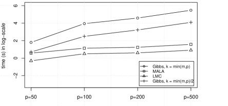
Resuts from our simulations in Table 1 and 2 show that our proposed algortihms (LMC and MALA) perform quite similar to the Gibbs sampler. However, it is shown that LMC and MALA are much more faster than the Gibbs sampler, see Figure 1. More specifically, we compare the running time of the LMC, MALA against the Gibbs sampler with and , in which we fixed and is varied by .
3.3 Real application to Image inpainting
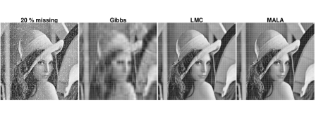
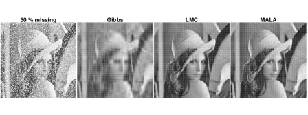
We further applied our proposed algorithms on image inpainting to evaluate their performance on real data. The aim of image inpainting is to complete an image with missing pixels. Here, we applied our methods on the well-known benchmark image Lena Gonzalez and Woods (2007) which is of size . This data has been used before in the context of matrix completion in Yang et al. (2018). The LMC and MALA are initialized from an output from the SoftImpute method in Mazumder et al. (2010) which is available in You (2020); Hastie and Mazumder (2015).
We consider the cases where and of pixels are missing uniformly at random. The experiments are repeated 30 times and the average of the considered errors is reported. The original Lena image with missing pixels and these images recovered by respective algorithms and the estimation errors results are given in Table 3.
From the results in Table 3 and Figure 2, we see that our proposed methods outperform the method based on Gibbs sampler. This can be explained as that the Gibbs sampler algorithm based on Gaussian low-rank factorizaton prior where all the entries of the image’s matrix are positive and thus the Gaussian low-rank factorizaton prior may not be an appropriate prior for image inpainting. On the other hand, our approach indicates that the spectral scaled student prior can capture the (apprioximate) low-rank structure and the smoothness of the image data matrix and as a consequence it helps obtain a better visual quality image, see Figure 2.
4 Conclusion
In this paper, we have studied the problem of Bayesian matrix completion by using a spectral scaled Student prior to promoting the low-rank structure of the underlying matrix. We have provided a thorough theoretical evaluation for our Bayesian estimator under both model misspecification and general sampling distribution. We have also provided efficient gradient-based sampling algorithms for our estimator by using Langevin Monte Carlo approach. These attractive features of our inference strategy are demonstrated through numerical simulations and real application to image inpainting.
Acknowledgements
TTM is supported by the Norwegian Research Council grant number 309960 through the Centre for Geophysical Forecasting at NTNU. I would like to warmly thank the anonymous referees for their useful comments on this work.
| Errors | Gibbs | LMC | MALA | Gibbs | LMC | MALA |
|---|---|---|---|---|---|---|
| MSE | 5.220 (.355) | 5.223 (.355) | 5.222 (.355) | 13.101 (.580) | 13.103 (.580) | 13.103 (.580) |
| NMSE | 2.715 (.470) | 2.717 (.470) | 2.716 (.470) | 2.644 (.309) | 2.644 (.309) | 2.644 (.309) |
| Pred | 5.548 (.498) | 5.550 (.498) | 5.550 (.498) | 14.934 (.890) | 14.936 (.890) | 14.935 (.890) |
| LMC | MALA | Gibbs | LMC | MALA | Gibbs | |
| MSE | 8.821 (.629) | 8.822 (.629) | 8.822 (.629) | 23.890 (1.158) | 23.893 (1.159) | 23.891 (1.158) |
| NMSE | 4.496 (.766) | 4.497 (.766) | 4.496 (.766) | 4.816 (.520) | 4.815 (.520) | 4.815 (.520) |
| Pred | 9.403 (.758) | 9.406 (.758) | 9.405 (.758) | 27.222 (1.560) | 27.225 (1.562) | 27.223 (1.559) |
| LMC | MALA | Gibbs | LMC | MALA | Gibbs | |
| MSE | 2.954 (.295) | 2.955 (.295) | 2.954 (.295) | 15.615 (2.593) | 15.616 (2.593) | 15.616 (2.593) |
| NMSE | 1.538 (.288) | 1.538 (.288) | 1.538 (.288) | 3.081 (.581) | 3.081 (.581) | 3.081 (.581) |
| Pred | 3.146 (.340) | 3.146 (.340) | 3.146 (.340) | 17.685 (2.999) | 17.685 (2.999) | 17.685 (2.999) |
| LMC | MALA | Gibbs | LMC | MALA | Gibbs | |
| MSE | 3.092 (.132) | 3.092 (.132) | 3.092 (.132) | 7.763 (.202) | 7.764 (.202) | 7.763 (.202) |
| NMSE | 1.554 (.189) | 1.554 (.189) | 1.554 (.189) | 1.554 (.101) | 1.554 (.101) | 1.554 (.101) |
| Pred | 3.222 (.153) | 3.223 (.153) | 3.222 (.153) | 8.445 (.260) | 8.446 (.260) | 8.446 (.260) |
| LMC | MALA | Gibbs | LMC | MALA | Gibbs | |
| MSE | 5.131 (.234) | 5.131 (.234) | 5.131 (.234) | 13.270 (.393) | 13.270 (.393) | 13.270 (.393) |
| NMSE | 2.657 (.298) | 2.657 (.298) | 2.657 (.298) | 2.648 (.208) | 2.648 (.208) | 2.648 (.208) |
| Pred | 5.369 (.261) | 5.369 (.261) | 5.369 (.261) | 14.411 (.472) | 14.411 (.472) | 14.411 (.472) |
| LMC | MALA | Gibbs | LMC | MALA | Gibbs | |
| MSE | 1.512 (.065) | 1.512 (.065) | 1.512 (.065) | 4.6974 (.1718) | 4.6975 (.1718) | 4.6974 (.1718) |
| NMSE | 0.766 (.077) | 0.766 (.077) | 0.766 (.077) | .9416 (.0756) | .9417 (.0756) | .9417 (.0756) |
| Pred | 1.582 (.074) | 1.582 (.074) | 1.582 (.074) | 5.0958 (.2001) | 5.0959 (.2001) | 5.0959 (.2001) |
| approximate rank-2, | approximate rank-5, | |||||
|---|---|---|---|---|---|---|
| Errors | Gibbs | LMC | MALA | Gibbs | LMC | MALA |
| MSE | 5.347 (.168) | 5.347 (.168) | 5.347 (.168) | 5.933 (.128) | 5.933 (.128) | 5.933 (.128) |
| NMSE | 2.254 (.244) | 2.255 (.244) | 2.254 (.244) | 1.079 (.086) | 1.079 (.086) | 1.079 (.086) |
| Pred | 5.803 (.266) | 5.804 (.266) | 5.804 (.266) | 7.112 (.295) | 7.112 (.295) | 7.112 (.295) |
| approximate rank-2, | approximate rank-5, | |||||
| LMC | MALA | Gibbs | LMC | MALA | Gibbs | |
| MSE | 5.936 (.188) | 5.936 (.188) | 5.936 (.188) | 7.388 (.205) | 7.389 (.205) | 7.388 (.205) |
| NMSE | 2.476 (.311) | 2.476 (.311) | 2.476 (.311) | 1.320 (.107) | 1.321 (.107) | 1.321 (.107) |
| Pred | 6.424 (.253) | 6.424 (.253) | 6.424 (.253) | 8.765 (.293) | 8.765 (.293) | 8.766 (.293) |
| approximate rank-2 | approximate rank-5 | |||||
| LMC | MALA | Gibbs | LMC | MALA | Gibbs | |
| MSE | 8.506 (.374) | 8.507 (.374) | 8.506 (.374) | 19.529 (2.150) | 19.529 (2.150) | 19.529 (2.150) |
| NMSE | 3.466 (.404) | 3.467 (.404) | 3.466 (.404) | 3.592 (.516) | 3.593 (.516) | 3.593 (.516) |
| Pred | 9.095 (.431) | 9.096 (.431) | 9.095 (.431) | 22.199 (2.472) | 22.200 (2.472) | 22.200 (2.472) |
| approximate rank-2 | approximate rank-5 | |||||
| LMC | MALA | Gibbs | LMC | MALA | Gibbs | |
| MSE | 5.181 (.110) | 5.181 (.110) | 5.181 (.110) | 5.446 (.124) | 5.446 (.124) | 5.446 (.124) |
| NMSE | 2.090 (.181) | 2.090 (.181) | 2.090 (.181) | 0.998 (.076) | 0.998 (.076) | 0.998 (.076) |
| Pred | 5.460 (.142) | 5.460 (.142) | 5.460 (.142) | 6.177 (.145) | 6.177 (.145) | 6.177 (.145) |
| approximate rank-2 | approximate rank-5 | |||||
| LMC | MALA | Gibbs | LMC | MALA | Gibbs | |
| MSE | 5.488 (.109) | 5.488 (.109) | 5.488 (.109) | 6.339 (.146) | 6.339 (.146) | 6.339 (.146) |
| NMSE | 2.206 (.178) | 2.206 (.178) | 2.206 (.178) | 1.167 (.074) | 1.168 (.074) | 1.167 (.074) |
| Pred | 5.762 (.128) | 5.762 (.128) | 5.762 (.128) | 7.087 (.182) | 7.087 (.182) | 7.087 (.182) |
| approximate rank-2, | approximate rank-5, | |||||
| LMC | MALA | Gibbs | LMC | MALA | Gibbs | |
| MSE | 6.805 (.175) | 6.806 (.175) | 6.806 (.175) | 10.648 (.240) | 10.648 (.240) | 10.648 (.240) |
| NMSE | 2.776 (.278) | 2.776 (.278) | 2.776 (.278) | 1.957 (.139) | 1.957 (.139) | 1.957 (.139) |
| Pred | 7.106 (.200) | 7.107 (.200) | 7.106 (.200) | 11.666 (.285) | 11.667 (.285) | 11.666 (.285) |
| Errors | Gibbs | LMC | MALA | Gibbs | LMC | MALA |
|---|---|---|---|---|---|---|
| MSE | 382.51 (1.37) | 136.91 (2.32) | 136.91 (2.32) | 350.91 (0.33) | 28.23 (.71) | 28.23 (.71) |
| Rank | 3.93 (0.25) | 3 (0) | 3 (0) | 3.5 (0.5) | 3 (0) | 3 (0) |
| NMSE | .0216 (.0001) | .0077 (.0001) | .0077 (.0001) | .01989 () | .00160 () | .00160 () |
| Pred | 453.95 (4.09) | 273.10 (4.56) | 273.10 (4.56) | 415.38 (7.41) | 139.49 (3.28) | 139.49 (3.28) |
References
- Adomavicius and Tuzhilin (2011) Gediminas Adomavicius and Alexander Tuzhilin. Context-aware recommender systems. In Recommender systems handbook, pages 217–253. Springer, 2011.
- Alquier (2013) P. Alquier. Bayesian methods for low-rank matrix estimation: short survey and theoretical study. In Algorithmic Learning Theory 2013, pages 309–323. Springer, 2013.
- Alquier et al. (2014) P. Alquier, V. Cottet, N. Chopin, and J. Rousseau. Bayesian matrix completion: prior specification and consistency. arXiv preprint arXiv:1406.1440, 2014.
- Alquier and Lounici (2011) Pierre Alquier and Karim Lounici. PAC-Bayesian bounds for sparse regression estimation with exponential weights. Electron. J. Stat., 5:127–145, 2011. ISSN 1935-7524. 10.1214/11-EJS601. URL http://dx.doi.org/10.1214/11-EJS601.
- Alquier and Ridgway (2020) Pierre Alquier and James Ridgway. Concentration of tempered posteriors and of their variational approximations. The Annals of Statistics, 48(3):1475–1497, 2020.
- Alquier et al. (2016) Pierre Alquier, James Ridgway, and Nicolas Chopin. On the properties of variational approximations of gibbs posteriors. The Journal of Machine Learning Research, 17(1):8374–8414, 2016.
- Babacan et al. (2012) S Derin Babacan, Martin Luessi, Rafael Molina, and Aggelos K Katsaggelos. Sparse bayesian methods for low-rank matrix estimation. IEEE Transactions on Signal Processing, 60(8):3964–3977, 2012.
- Bennett and Lanning (2007) J. Bennett and S. Lanning. The netflix prize. In Proceedings of KDD cup and workshop, volume 2007, page 35, 2007.
- Bhattacharya et al. (2019) Anirban Bhattacharya, Debdeep Pati, Yun Yang, et al. Bayesian fractional posteriors. Annals of Statistics, 47(1):39–66, 2019.
- Bissiri et al. (2016) Pier Giovanni Bissiri, Chris C Holmes, and Stephen G Walker. A general framework for updating belief distributions. Journal of the Royal Statistical Society. Series B, Statistical methodology, 78(5):1103, 2016.
- Cabral et al. (2014) Ricardo Cabral, Fernando De la Torre, Joao Paulo Costeira, and Alexandre Bernardino. Matrix completion for weakly-supervised multi-label image classification. IEEE transactions on pattern analysis and machine intelligence, 37(1):121–135, 2014.
- Candès and Plan (2010) E. J. Candès and Y. Plan. Matrix completion with noise. Proceedings of the IEEE, 98(6):925–936, 2010.
- Candès and Recht (2009) Emmanuel J. Candès and Benjamin Recht. Exact matrix completion via convex optimization. Found. Comput. Math., 9(6):717–772, 2009. ISSN 1615-3375. 10.1007/s10208-009-9045-5. URL http://dx.doi.org/10.1007/s10208-009-9045-5.
- Candès and Tao (2010) Emmanuel J. Candès and Terence Tao. The power of convex relaxation: near-optimal matrix completion. IEEE Trans. Inform. Theory, 56(5):2053–2080, 2010. ISSN 0018-9448. 10.1109/TIT.2010.2044061. URL http://dx.doi.org/10.1109/TIT.2010.2044061.
- Candes et al. (2008) Emmanuel J Candes, Michael B Wakin, and Stephen P Boyd. Enhancing sparsity by reweighted minimization. Journal of Fourier analysis and applications, 14(5-6):877–905, 2008.
- Catoni (2004) O. Catoni. Statistical learning theory and stochastic optimization, volume 1851 of Saint-Flour Summer School on Probability Theory 2001 (Jean Picard ed.), Lecture Notes in Mathematics. Springer-Verlag, Berlin, 2004. ISBN 3-540-22572-2. 10.1007/b99352. URL http://dx.doi.org/10.1007/b99352.
- Catoni (2007) O. Catoni. PAC-Bayesian supervised classification: the thermodynamics of statistical learning. Institute of Mathematical Statistics Lecture Notes—Monograph Series, 56. Institute of Mathematical Statistics, Beachwood, OH, 2007. ISBN 978-0-940600-72-0; 0-940600-72-2.
- Chen et al. (2019) Yuxin Chen, Jianqing Fan, Cong Ma, and Yuling Yan. Inference and uncertainty quantification for noisy matrix completion. Proceedings of the National Academy of Sciences, 116(46):22931–22937, 2019.
- Chi et al. (2013) Eric C Chi, Hua Zhou, Gary K Chen, Diego Ortega Del Vecchyo, and Kenneth Lange. Genotype imputation via matrix completion. Genome research, 23(3):509–518, 2013.
- Corander and Villani (2004) Jukka Corander and Mattias Villani. Bayesian assessment of dimensionality in reduced rank regression. Statistica Neerlandica, 58(3):255–270, 2004.
- Cottet and Alquier (2018) Vincent Cottet and Pierre Alquier. 1-bit matrix completion: Pac-bayesian analysis of a variational approximation. Machine Learning, 107(3):579–603, 2018.
- Dalalyan and Tsybakov (2008) Arnak Dalalyan and Alexandre B Tsybakov. Aggregation by exponential weighting, sharp pac-bayesian bounds and sparsity. Machine Learning, 72(1-2):39–61, 2008.
- Dalalyan (2020) Arnak S Dalalyan. Exponential weights in multivariate regression and a low-rankness favoring prior. Annales de l’Institut Henri Poincaré, Probabilités et Statistiques, 56(2):1465–1483, 2020.
- Dalalyan and Karagulyan (2019) Arnak S Dalalyan and Avetik Karagulyan. User-friendly guarantees for the langevin monte carlo with inaccurate gradient. Stochastic Processes and their Applications, 129(12):5278–5311, 2019.
- Dalalyan and Tsybakov (2012) Arnak S Dalalyan and Alexandre B Tsybakov. Sparse regression learning by aggregation and langevin monte-carlo. Journal of Computer and System Sciences, 78(5):1423–1443, 2012.
- Durmus and Moulines (2019) Alain Durmus and Eric Moulines. High-dimensional bayesian inference via the unadjusted langevin algorithm. Bernoulli, 25(4A):2854–2882, 2019.
- Foygel et al. (2011) Rina Foygel, Ohad Shamir, Nati Srebro, and Ruslan Salakhutdinov. Learning with the weighted trace-norm under arbitrary sampling distributions. In Advances in Neural Information Processing Systems, pages 2133–2141, 2011.
- Friedman et al. (2010) Jerome Friedman, Trevor Hastie, and Robert Tibshirani. Regularization paths for generalized linear models via coordinate descent. Journal of Statistical Software, 33(1):1–22, 2010. URL https://www.jstatsoft.org/v33/i01/.
- Geweke (1996) John Geweke. Bayesian reduced rank regression in econometrics. Journal of econometrics, 75(1):121–146, 1996.
- Gonzalez and Woods (2007) Rafael C Gonzalez and Richard E Woods. Digital image processing. Prentice hall Upper Saddle River, NJ, 2007.
- Gross et al. (2010) David Gross, Yi-Kai Liu, Steven T Flammia, Stephen Becker, and Jens Eisert. Quantum state tomography via compressed sensing. Physical review letters, 105(15):150401, 2010.
- Grünwald and Van Ommen (2017) Peter Grünwald and Thijs Van Ommen. Inconsistency of bayesian inference for misspecified linear models, and a proposal for repairing it. Bayesian Analysis, 12(4):1069–1103, 2017.
- Guedj and Robbiano (2018) Benjamin Guedj and Sylvain Robbiano. Pac-bayesian high dimensional bipartite ranking. Journal of Statistical Planning and Inference, 196:70–86, 2018.
- Hastie and Mazumder (2015) Trevor Hastie and Rahul Mazumder. softImpute: Matrix Completion via Iterative Soft-Thresholded SVD, 2015. URL https://CRAN.R-project.org/package=softImpute. R package version 1.4.
- Hastie et al. (2015) Trevor Hastie, Rahul Mazumder, Jason D Lee, and Reza Zadeh. Matrix completion and low-rank svd via fast alternating least squares. The Journal of Machine Learning Research, 16(1):3367–3402, 2015.
- He and Sun (2014) Kaiming He and Jian Sun. Image completion approaches using the statistics of similar patches. IEEE transactions on pattern analysis and machine intelligence, 36(12):2423–2435, 2014.
- Jiang et al. (2016) Bo Jiang, Shiqian Ma, Jason Causey, Linbo Qiao, Matthew Price Hardin, Ian Bitts, Daniel Johnson, Shuzhong Zhang, and Xiuzhen Huang. Sparrec: An effective matrix completion framework of missing data imputation for gwas. Scientific reports, 6(1):1–15, 2016.
- Kleibergen and Paap (2002) Frank Kleibergen and Richard Paap. Priors, posteriors and bayes factors for a bayesian analysis of cointegration. Journal of Econometrics, 111(2):223–249, 2002.
- Klopp (2014) Olga Klopp. Noisy low-rank matrix completion with general sampling distribution. Bernoulli, 20(1):282–303, 2014. ISSN 1350-7265. 10.3150/12-BEJ486. URL http://dx.doi.org/10.3150/12-BEJ486.
- Klopp (2015) Olga Klopp. Matrix completion by singular value thresholding: sharp bounds. Electronic journal of statistics, 9(2):2348–2369, 2015.
- Koltchinskii et al. (2011) Vladimir Koltchinskii, Karim Lounici, and Alexandre B. Tsybakov. Nuclear-norm penalization and optimal rates for noisy low-rank matrix completion. Ann. Statist., 39(5):2302–2329, 2011. ISSN 0090-5364. 10.1214/11-AOS894. URL http://dx.doi.org/10.1214/11-AOS894.
- Lawrence and Urtasun (2009) N. D Lawrence and R. Urtasun. Non-linear matrix factorization with gaussian processes. In Proceedings of the 26th Annual International Conference on Machine Learning, pages 601–608. ACM, 2009.
- Lim and Teh (2007) Y. J. Lim and Y. W. Teh. Variational bayesian approach to movie rating prediction. In Proceedings of KDD Cup and Workshop, volume 7, pages 15–21, 2007.
- Luo et al. (2015) Yong Luo, Tongliang Liu, Dacheng Tao, and Chao Xu. Multiview matrix completion for multilabel image classification. IEEE Transactions on Image Processing, 24(8):2355–2368, 2015.
- Mai (2021a) The Tien Mai. Efficient bayesian reduced rank regression using langevin monte carlo approach. arXiv preprint arXiv:2102.07579, 2021a.
- Mai (2021b) The Tien Mai. Numerical comparisons between bayesian and frequentist low-rank matrix completion: estimation accuracy and uncertainty quantification. arXiv preprint arXiv:2103.11749, 2021b.
- Mai and Alquier (2015) The Tien Mai and Pierre Alquier. A bayesian approach for noisy matrix completion: Optimal rate under general sampling distribution. Electron. J. Statist., 9(1):823–841, 2015. 10.1214/15-EJS1020. URL https://doi.org/10.1214/15-EJS1020.
- Mai and Alquier (2017) The Tien Mai and Pierre Alquier. Pseudo-bayesian quantum tomography with rank-adaptation. Journal of Statistical Planning and Inference, 184:62–76, 2017.
- Mazumder et al. (2010) Rahul Mazumder, Trevor Hastie, and Robert Tibshirani. Spectral regularization algorithms for learning large incomplete matrices. The Journal of Machine Learning Research, 11:2287–2322, 2010.
- McAllester (1998) D.A. McAllester. Some PAC-Bayesian theorems. In Proceedings of the Eleventh Annual Conference on Computational Learning Theory, pages 230–234, New York, 1998. ACM.
- Negahban and Wainwright (2012) Sahand Negahban and Martin J. Wainwright. Restricted strong convexity and weighted matrix completion: optimal bounds with noise. J. Mach. Learn. Res., 13:1665–1697, 2012. ISSN 1532-4435.
- Recht and Ré (2013) Benjamin Recht and Christopher Ré. Parallel stochastic gradient algorithms for large-scale matrix completion. Math. Program. Comput., 5(2):201–226, 2013. ISSN 1867-2949. 10.1007/s12532-013-0053-8. URL http://dx.doi.org/10.1007/s12532-013-0053-8.
- Ridgway et al. (2014) James Ridgway, Pierre Alquier, Nicolas Chopin, and Feng Liang. Pac-bayesian auc classification and scoring. In Proceedings of the 27th International Conference on Neural Information Processing Systems-Volume 1, pages 658–666, 2014.
- Roberts and Rosenthal (1998) Gareth O Roberts and Jeffrey S Rosenthal. Optimal scaling of discrete approximations to langevin diffusions. Journal of the Royal Statistical Society: Series B (Statistical Methodology), 60(1):255–268, 1998.
- Roberts and Stramer (2002) Gareth O Roberts and Osnat Stramer. Langevin diffusions and metropolis-hastings algorithms. Methodology and computing in applied probability, 4(4):337–357, 2002.
- Salakhutdinov and Mnih (2008) R. Salakhutdinov and A. Mnih. Bayesian probabilistic matrix factorization using markov chain monte carlo. In Proceedings of the 25th international conference on Machine learning, pages 880–887. ACM, 2008.
- Shawe-Taylor and Williamson (1997) J. Shawe-Taylor and R. Williamson. A PAC analysis of a Bayes estimator. In Proceedings of the Tenth Annual Conference on Computational Learning Theory, pages 2–9, New York, 1997. ACM.
- Xiong et al. (2010) Liang Xiong, Xi Chen, Tzu-Kuo Huang, Jeff Schneider, and Jaime G Carbonell. Temporal collaborative filtering with bayesian probabilistic tensor factorization. In Proceedings of the 2010 SIAM international conference on data mining, pages 211–222. SIAM, 2010.
- Yang et al. (2018) Linxiao Yang, Jun Fang, Huiping Duan, Hongbin Li, and Bing Zeng. Fast low-rank bayesian matrix completion with hierarchical gaussian prior models. IEEE Transactions on Signal Processing, 66(11):2804–2817, 2018.
- You (2020) Kisung You. filling: Matrix Completion, Imputation, and Inpainting Methods, 2020. URL https://CRAN.R-project.org/package=filling. R package version 0.2.2.
- Zhou et al. (2010) M. Zhou, C. Wang, M. Chen, J. Paisley, D. Dunson, and L. Carin. Nonparametric bayesian matrix completion. Proc. IEEE SAM, 2010.
Appendix A Appendix
A.1 Brief review on futher related works
It is worth noting that most studies in matrix completion consider that the sampling distribution is uniform, see Alquier et al. (2014); Candès and Plan (2010); Candès and Recht (2009); Candès and Tao (2010); Koltchinskii et al. (2011); Alquier and Ridgway (2020); Lim and Teh (2007) among others. However, in practice the observed entries are not assured to be uniformly distributed: for example, some items are more popular and as a consequence receive much more ratings than others. More importantly, it is noted that the sampling distribution is usually not known in practice. Several studies have been performed for general sampling schemes rather than uniform distribution, see e.g. Foygel et al. (2011); Klopp (2014); Negahban and Wainwright (2012). Moreover, the paper Mai and Alquier (2015) is the first line of works that studied (Bayesian) matrix completion under a general sampling model without any restriction.
The spectral scaled Student prior has been considered before in the context of image denoising Dalalyan (2020) and in reduced rank regression Mai (2021a). Moreover, it is shown that if a random matrix has the density distribution as in (3), then the random vectors are all drawn from the -variate scaled Student distribtuion , (Dalalyan, 2020, Lemma 1). On the other hand, this prior can be seen as the marginal distribution of the Gaussian-inverse Wishart prior that is explored in Yang et al. (2018) in the context of matrix completion where the precision matrix is integrated out. Therefore, in some ways, our work provide theoretical assessment for that paper. However, we note that the paper Yang et al. (2018) consider an opimization approach to Bayesian matrix completion using variational inference while our work propose an efficient sampling approach.
A.2 Short review on low-rank factorization priors
Up to our knowledge, the paper Geweke (1996) was the first work that introduced a low-rank factorization prior in a context of low-rank matrix estimation. The idea is to express the matrix as with and then the prior is difined on and rather than on as
for some . This approach has been used in matrix completion for the first time in Lim and Teh (2007). However, this approach is faced with the problem of choosing . One could perform model selection for any possible as done in Kleibergen and Paap (2002); Corander and Villani (2004) but the computation may be expensive for large data set. Recent approaches as in Babacan et al. (2012) focus on fixing a large , e.g. , then sparsity-promoting priors are placed on the columns of and such that most columns are almost null. As a consequence, the resulting matrix is approximately low-rank. See Alquier (2013); Alquier et al. (2014) for the details and dicussions on low-rank factorization priors.
Using low-rank factorization priors, most authors use the Gibbs sampler to simulate from the posterior as the conditional posterior distributions can be derived explitcitely, e.g. in Salakhutdinov and Mnih (2008). However, it is noted that these Gibbs sampling algorithms update the factor matrices in a row-by-row manner and invole a number of matrix inverse or singular value decomposition operations at each iteration. This is expensive and slow down the algorithm for large data set significantly.
A.3 Theoretical result in special cases: uniformly sampling and exact low-rank
Firstly, when the sampling distribution is uniform, we obtain the following result for the Frobenius norm directly from Theorem 2.1.
Corollary A.1.
Secondly, as soon as the true matrix is low-rank where its rank is atmost , we can pick and obtain the following results.
A.4 A Metropolis-adjusted Langevin algorithm
Here, we propose a Metropolis-Hasting correction to the LMC. This approach guarantees the convergence to the posterior and it also provides a useful way for choosing . More precisely, we consider the update rule in (5) as a proposal for a new state,
| (7) |
Note that is normally distributed with mean and the covariance matrices equal to times the identity matrices. This proposal is accepted or rejected according to the Metropolis-Hastings algorithm that the proposal is accepted with probabiliy:
where
is the transition probability density from to . Compared to random-walk Metropolis–Hastings, the advantage of MALA is that it usually proposes moves into regions of higher probability, which are then more likely to be accepted.
We note that the step-size is chosen such that the acceptance rate is approximate following Roberts and Rosenthal (1998). See Section 3.2 for some choices in special cases in our simulations.
It is also noted that an immediate application of the LMC algorithm in (5) needs to calculate a matrix inversion at each iteration. This might be expensive and can slow down significantly the algorithm. Therefore, in the case of very big data or huge , we could replace this matrix inversion by its accurately approximation through a convex optimization. More precisely, it can be easily verified that the matrix is the solution to the following convex optimization problem
The solution of this optimization problem can be conveniently obtained by using the package ’glmnet’ Friedman et al. (2010) (with family option ’mgaussian’). This avoid to perform matrix inversion or other costly calculation. However, we note here that the LMC algorithm is being used with approximate gradient evaluation, theoretical assessment of this approach can be found in Dalalyan and Karagulyan (2019).
A.5 Proofs
The main argument of the proof is based on the so-called PAC-Bayesian bounds which were introduced in Shawe-Taylor and Williamson (1997); McAllester (1998). However, our results are derived by following the Catoni’s works Catoni (2007) where the author shown how to derive powerful oracle inequalities from PAC-Bayesian bounds. Since then this technique has been use many times to obtain oracle inequalities in many different problems Dalalyan and Tsybakov (2008); Mai and Alquier (2015); Alquier and Lounici (2011); Guedj and Robbiano (2018); Ridgway et al. (2014); Cottet and Alquier (2018); Mai and Alquier (2017); Alquier et al. (2016)
For the sake of simplicity, let us define
In order to understand what follows, keep in mind that our optimal estimator comes with , so and are of order .
First, we state a general PAC-Bayesian inequality for matrix completion from Mai and Alquier (2015), in the style of Catoni (2004); Dalalyan and Tsybakov (2008).
Theorem A.3.
This theorem is the result from the Step 1 in the proof of Theorem 1 in Mai and Alquier (2015).
Now, we are ready to present the proof of Theorem 2.1.
Proof A.4 ( of Theorem 2.1).
Let’s fix an arbitrary matrix . Let be the distribution obtained from the prior by a translation
Now, we apply Theorem A.3 and upper bound the right hand side of (8) evaluated at the distribution . We obtain
Firstly, we deal with the integral term that
By using the translation invariance of the Lebesgue measure and the fact that , we obtain
For the last integral, we have that
using the Lemma 1 in Dalalyan (2020).
Secondly, we deal with the Kullback-Leibler term. We have that
that is followed by using Lemma 2 in Dalalyan (2020).
Therefore, we have for any matrix with that
| (9) |
Taking now with , we get that with , and that . Thus, the inequality (A.4) yeilds
Now, by taking , we obtain that
where is a universal constants that depends on only.
This completes the proof of the theorem.