Calculation of generating function in many-body systems with quantum computers: technical challenges and use in hybrid quantum-classical methods

Abstract

The generating function of a Hamiltonian $H$ is defined as $F(t)=\langle e^{-itH}\rangle$, where $t$ is the time and where the expectation value is taken on a given initial quantum state. This function gives access to the different moments of the Hamiltonian $\langle H^{K}\rangle$ at various orders $K$. The real and imaginary parts of $F(t)$ can be respectively evaluated on quantum computers using one extra ancillary qubit with a set of measurement for each value of the time $t$. The low cost in terms of qubits renders it very attractive in the near term period where the number of qubits is limited. Assuming that the generating function can be precisely computed using quantum devices, we show how the information content of this function can be used a posteriori on classical computers to solve quantum many-body problems. Several methods of classical post-processing are illustrated with the aim to predict approximate ground or excited state energies and/or approximate long-time evolutions. This post-processing can be achieved using methods based on the Krylov space and/or on the $t$-expansion approach that is closely related to the imaginary time evolution. Hybrid quantum-classical calculations are illustrated in many-body interacting systems using the pairing and Fermi-Hubbard models.

I Introduction

With recent advances in the development of quantum computing (QC) platforms, the possibility of exploiting quantum devices for realistic simulations of complex quantum systems, as suggested by Feynman Fey82 , is becoming a reality (see for instance Aru19 ; Ale21 ). Nowadays, quantum simulations are possible, but the quantum noise and decoherence significantly limit the number of operations that could be performed efficiently on existing platforms. This is what nowadays is called the NISQ (Noisy Intermediate-Scale Quantum) era Pre18 where simulations on quantum computers are possible but the algorithms and tasks should adapt to noise. Because of this noise, many standard algorithms cannot be used in actual QC devices while others appear particularly suited in the NISQ context. In the present work, we are interested in simulating complex quantum systems. In this context, a typical example of NISQ ”friendly” strategy is the use of Variational optimizers using Hybrid quantum-classical architectures where the optimization is made with a classical computer End21 ; Cer21 . These developments have given a strong impulse to the use of quantum computers for calculating complex quantum many-body systems in different fields of physics Lan10 ; Bab15 ; OMa16 ; Col18 ; Hem18 ; Mac18 ; Dum18 ; Lu19 ; Rog19 ; Du20 ; Klc18 ; Klc19 ; Ale19 ; Lam19 . For recent reviews on the subject see for instance Mcc17 ; Fan19 ; Cao19 ; McA20 ; Bau20 ; Bha21 .

Here, we explore a different hybrid strategy to simulate quantum systems. Our starting hypothesis is that the QC can simulate the evolution of a quantum system, at least approximately, over a restricted time interval $[0,t_{{\rm max}}]$. The method we propose can be seen as a natural generalization of the one used in Refs. Kni07 ; Rog20 where the expectation value of an Hermitian operator $O$ is replaced by the evolution of the operator $e^{-itO}$ over a short time interval. Here, we use the standard concept of generating function. The generating function is already used implicitly in the context of quantum computing in the quantum phase estimation (QPE) algorithm Nie02 . It was exploited recently in Ref. Lac20 to restore symmetries in many-body systems. However, in this case, the circuit is too deep to be simulated in the NISQ period. Here, we show that the generating function (GF) can be obtained using a single ancillary qubit. Precise estimates of the GF gives a priori access to set of moments $\langle H^{K}\rangle$ with $K\leq M$ using the GF. This technique was already discussed in Ref. Pen21 ; Cla21 in combination with variational principles and noted as a possible tool for the NISQ period. We give illustration here of methods where the moments can be used in a second step for a post-processing on a classical computer to study the static and dynamical properties of complex systems.

II Generating function on quantum computers and $\langle H^{K}\rangle$ estimates

The generating function is a standard concept of classical probability and statistical theory. We recall briefly here how this concept can be exploited in quantum systems Bal07 . We consider a system described by a density $\rho$. In the following, we assume implicitly that ${\rm Tr}(\rho)=1$. If the system is in a pure state, the density can be written as $\rho=|\Phi\rangle\langle\Phi|$.

For a given operator $O$, we can define the generating function as:

$$F(\gamma) = {\rm Tr}\left(e^{\gamma O}\rho\right),$$ (1)

where $\gamma$ is a complex number. The interest of the generating function is that its knowledge gives access to the different non-centered moments $\langle O^{K}\rangle={\rm Tr}(O^{K}\rho)$ associated to the density $\rho$. Indeed, expanding the exponential, we deduce:

$$F(\gamma) = 1+\gamma\langle O\rangle+\frac{\gamma^{2}}{2!}\langle O^{2}\rangle+\cdots$$ (2)

that corresponds to the Taylor expansion of $F(\gamma)$ with the condition:

$$\left.\frac{d^{K}F(\gamma)}{d\gamma^{K}}\right|_{\gamma=0} = \langle O^{K}\rangle.$$ (3)

Until now, we have not specified $\gamma$. Our aim is to estimate the generating function on a quantum computer. Since quantum computers are convenient to perform unitary evolutions, it is suitable to take $\gamma=-it$. Then, if $O$ is Hermitian, $e^{-itO}$ is a unitary operator.

We will focus our attention here on the case where $O$ identifies with a Hamiltonian denoted by $H$. Assuming $\hbar=1$, the operator entering in Eq. (1) is simply the propagator in time $U(t)=e^{-itH}$. In practice, the simulation of non-unitary (but Hermitian) operators, such as the Hamiltonian or its powers, on a quantum computer is a much more complicated task than performing $U(t)$ itself (see for instance the discussion in Ber15 ). The GF provides a practical tool to estimate the expectation values of such non-unitary operators while performing only unitary operations.

The GF is already used explicitly or implicitly in the quantum computing context. For instance, the quantum phase-estimation (QPE) approach Nie02 ; Hid19 ; Fan19 ; Ovr03 ; Ovr07 applied to an operator $U_{S}=e^{2\pi iS}$ is actually computing the generating function associated to the operator $S$ on a set of ancillary qubits prior to performing the quantum inverse Fourier transform to obtain the probability distribution of the eigenstates of $S$. The GF is also a key ingredient of the time-series method discussed in Ref. Som19 .

Our strategy in the present work is to assign to the quantum computer solely the task of computing the GF, even on a restricted interval of time, with the additional constraint to minimize the number of ancillary qubits. The generating function is then transmitted as input to a classical computer for post-processing. We will give below several illustrations of such post-processing.

On a quantum computer, the GF can be obtained by adding a single register qubit to the ones used for the system itself. For a given value of $t$, the real and imaginary parts of $F(t)$ are obtained using the standard Hadamard test or the modified Hadamard test, as shown respectively in panels (a) and (b) of Fig. 1, by measuring the additional qubit. Note that, a set of measurements is required for each values of the time. Illustrations of generating functions are given below for interacting fermions.

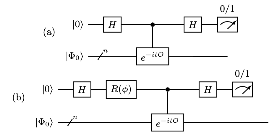
Figure 1: Illustration of the (a) Hadamard test and (b) modified Hadamard test that are used in the present work to compute respectively the real and imaginary parts of the GF for a given Hermitian operator $O$. In this circuit, $H$ is the standard Hadamard gate while $R(\phi)$ corresponds to the phase gate where the angle is set to $\phi=-\pi/2$. In the case (a), the probability to measure 0 or 1 on the ancillary qubit verifies $p_{0}-p_{1}={\rm Re}\{F(t)\}$ while in the case (b) we have $p_{0}-p_{1}={\rm Im}\{F(t)\}$. The circuits shown here and in the following figures have been made using the quantikz package of Ref. Kay18 .

II.1 Illustration of the method

To illustrate the method, we consider two different Hamiltonians that are standardly used to test many-body approaches, namely the pairing Hamiltonian and the one dimensional Fermi-Hubbard model. In both cases, we have used the Jordan-Wigner transformation (JWT) Jor28 ; Lie61 ; Som02 ; See12 ; Dum18 ; Fan19 to map the Hamiltonian written in second quantization into a set of interacting qubits. We take the following specific convention for the mapping. Assuming a set of fermion creation/annihilation operators $(a_{j}^{\dagger},a_{j})$, we map these operators into qubits gates such that

$$\left\{\begin{array}[]{l}a_{j}^{\dagger}\longrightarrow A_{j}^{+}=Z_{j-1}^{<}\otimes Q_{j}^{+}\\ \\ a_{j}\longrightarrow A_{j}=Z_{j-1}^{<}\otimes Q_{j}\end{array}\right.,$$ (7)

with the definitions

$$Q_{j}=\frac{1}{2}\left(X_{j}+iY_{j}\right),~{}~{}~{}Q_{j}^{+}=\frac{1}{2}\left(X_{j}-iY_{j}\right).$$ (8)

Here $(X_{j},Y_{j},Z_{j})$ are the standard Pauli matrices acting on the qubit $j$. We add to these operators the identity operator $I_{j}$. In the equation (7), we have defined the quantity $Z_{j-1}^{<}$ as

$$Z_{j-1}^{<} = \bigotimes_{k=0}^{j-1}(-Z_{k}).$$

With this convention we have for instance $Q_{j}^{+}|0_{j}\rangle=|1_{j}\rangle$ and $a_{k}^{\dagger}a_{k}\rightarrow N_{k}=(I_{k}-Z_{k})/2$. Basic aspects related to the quantum simulation of both model Hamiltonians considered here are summarized below.

II.1.1 Fermi-Hubbard model

The Fermi-Hubbard model is a widely used schematic model to describe interacting fermions on a lattice Jak98 ; Gre02 . The Hubbard Hamiltonian was already simulated on quantum computers in Ref. Wec15 ; Jia18 . We consider here the one-dimension Fermi-Hubbard model with sharp boundary conditions. The Hamiltonian describes a set of $N$ fermions with spins on a set of $M$ lattice sites which are labeled as $i=0,1,\dots,M-1$. This Hamiltonian is written as $H=H_{J}+H_{U}$, where $H_{J}$ and $H_{U}$ are the hopping and interaction terms respectively given by:

$$H_{J} = -J\sum_{i,\sigma}(a_{i+1,\sigma}^{\dagger}a_{i,\sigma}+a_{i,\sigma}^{\dagger}a_{i+1,\sigma}),$$

$$H_{U} = +U\sum_{i}\hat{n}_{i,\uparrow}\hat{n}_{i,\downarrow},$$

with $n_{i,\sigma}=a_{i,\sigma}^{\dagger}a_{i,\sigma}$ and $\sigma=\{\uparrow,\downarrow\}$. In order to apply the JWT mapping, it is convenient to organize the qubits as follows. Spin-up single-particle states indexed as $i=0,\dots,M-1$ are associated with qubits labeled with $\alpha=0,\dots,M-1$. Particles with spin-down indexed as $i=0,\dots,M-1$ are associated to qubits $\alpha=M,\dots,2M-1$. With this, we obtain the mapping (with proper account for the boundary conditions):

$$H_{J} = J\sum_{\alpha=0,\alpha\neq M-1}^{2M-2}\left[Q_{\alpha+1}^{+}Q_{\alpha}+{\rm h.c.}\right],$$

together with

$$H_{U}=\frac{U}{4}\sum_{\alpha=0,M-1}\left[I_{\alpha}-Z_{\alpha}\right]\left[I_{\alpha+M}-Z_{\alpha+M}\right].$$ (9)

The generating function evaluation with the circuits presented in Fig. 1 requires to perform the time-evolution operator. For its implementation, we simply use the Trotter-Suzuki method Tro59 ; McA20 . The time interval $[0,t]$ is divided into small intervals $\Delta t$. For small enough time interval, we have:

$$U(\Delta t)=e^{-i\Delta tH}\simeq e^{-i\Delta tH_{J}}e^{-i\Delta tH_{U}}\equiv U_{J}(\Delta t)U_{U}(\Delta t).$$

The propagators $U_{J}$ can be further decomposed as:

$$U_{J}(\Delta t) = \prod_{\alpha}e^{-iJ\Delta t\left[Q_{\alpha+1}^{+}Q_{\alpha}+{\rm h.c.}\right]},$$ (10)

$$= \prod_{\alpha}\begin{pmatrix}1&0&0&0\\ 0&\cos\left(\lambda\right)&-i\sin\left(\lambda\right)&0\\ 0&-i\sin\left(\lambda\right)&\cos\left(\lambda\right)&0\\ 0&0&0&1\end{pmatrix}_{\alpha,\alpha+1}$$

with $\lambda=\Delta tJ$. To obtain the matrix form, standard manipulation of Pauli matrices is used. Note that the index on the matrix indicates that the matrix acts on the two qubits $\alpha$ and $\alpha+1$.

For the interaction propagator we have

$$U_{U}(\Delta t) = \prod_{\alpha}e^{-iU\Delta t\left[I_{\alpha}-Z_{\alpha}\right]\left[I_{\alpha+M}-Z_{\alpha+M}\right]},$$ (11)

$$= \prod_{\alpha}\begin{pmatrix}1&0&0&0\\ 0&1&0&0\\ 0&0&1&0\\ 0&0&0&e^{-i\Delta tU}\end{pmatrix}_{\alpha,\alpha+M}.$$

We recognize in the last expression the controlled phase-shift gate with phase $\phi=-\Delta tU$. The two circuits that simulate $U_{U}$ and $U_{J}$ are displayed in panels (a) and (b) of Fig. 2.

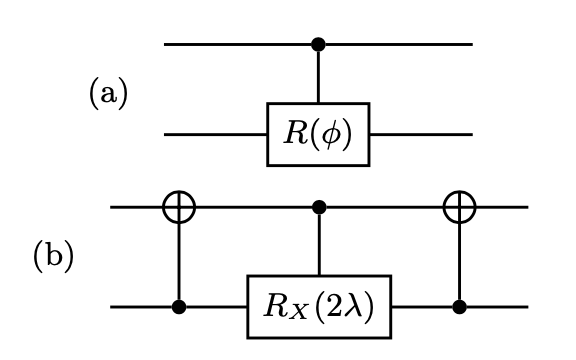
Figure 2: Circuits used to simulate the Hubbard model. The circuit (a) simulates the interaction term $H_{U}$ where $R(\phi)$ is the unitary phase operator with $\phi=-\Delta tU$. Circuit (b) simulates a short time-step evolution of the hopping term $H_{J}$ where $R_{X}(2\lambda)=e^{-i\lambda X}$ and where $\lambda=J\Delta t$.

II.1.2 Pairing Hamiltonian

As a second illustration, we will also consider the pairing Hamiltonian Von01 ; Zel03 ; Duk04 ; Bri05 that is standardly used in the context of nuclear physics or small superconducting systems. This Hamiltonian has already been used on QC in Refs. Ovr03 ; Ovr07 and more recently in Refs. Lac20 ; Kha21 . We write this Hamiltonian as:

$$H = \sum_{p}\varepsilon_{p}N_{p}+g\sum_{pq}P^{\dagger}_{p}P_{q}\equiv H_{\varepsilon}+H_{g}.$$ (12)

Introducing the notation $(a_{p}^{\dagger},a_{\bar{p}}^{\dagger})$ as the creation operators of time-reversed single-particle states. The different operators are defined as:

$$\hat{N}_{p} = a_{p}^{\dagger}a_{p}+a_{\bar{p}}^{\dagger}a_{\bar{p}},$$

$$\hat{P}_{p}^{\dagger} = a_{p}^{\dagger}a_{\bar{p}}^{\dagger}.$$

These operators correspond respectively to the pair occupation, and to the pair creation operators. In this model, time-reversed single-particle states are degenerated with energies $\widetilde{\varepsilon}_{p}=\varepsilon_{p}+g_{pp}/2$, where the $g_{pp}/2$ term is added to compensate from the shift induced by scattering of each pair by itself in the $H_{g}$ term (case $p=q$).

The mapping from fermions to qubit of the pairing problem can be made in different ways. In the most general situation, one can follow the standard JWT where one particle corresponds to one qubit. This was done for instance in Ref. Ovr07 or in Lac20 . The method to map fermions to qubits used in these works is general and can treat the case of system with odd or even particle numbers. We are interested here only in systems with even number of particles with the particularity that there is no broken pairs (seniority zero scheme Bri05 ), one can then directly map each pair operator $P_{p}^{\dagger}$ into a single qubit. This was done in Ref. Kha21 with the advantage to reduce the number of qubits needed to describe the system. Here, we use the latter strategy. Following Ref. Kha21 , the Hamiltonian in the qubits space is written as:

$$H = \sum_{p}\varepsilon_{p}\left[1-Z_{p}\right]-\frac{1}{2}\sum_{p>q}g_{pq}\left[X_{p}X_{q}+Y_{p}Y_{q}\right].$$ (13)

We apply the Trotter-Suzuki method to this Hamiltonian and denote by $U_{\varepsilon}(\Delta t)$ and $U_{g}(\Delta t)$ the propagator associated respectively to $H_{\varepsilon}$ and $H_{g}$ for small time-step evolution $\Delta t$. For the one-body part of the Hamiltonian, we have:

$$U_{\varepsilon}(\Delta t) = \prod_{p}\exp\left(-i\Delta t\varepsilon_{p}\left[1-Z_{p}\right]\right),$$ (16)

$$= \prod_{p}\left(\begin{array}[]{cc}1&0\\ 0&\exp\left(-2i\varepsilon_{p}\Delta t\right)\end{array}\right)\equiv\prod_{p}R(\phi_{p}),$$

where $R(\phi_{p})$ is the unitary phase-gate operator with $\phi_{p}=-2\varepsilon_{p}\Delta t$. For the interaction part, we have:

$$U_{g}(\Delta t) = \prod_{p>q}\exp\left(+ig_{pq}\frac{\Delta t}{2}\left[X_{p}X_{q}+Y_{p}Y_{q}\right]\right)$$ (17)

$$= \prod_{p>q}\begin{pmatrix}1&0&0&0\\ 0&\cos(\lambda_{pq})&i\sin(\lambda_{pq})&0\\ 0&i\sin(\lambda_{pq})&\cos(\lambda_{pq})&0\\ 0&0&0&1\end{pmatrix}.$$

where we have defined $\lambda_{pq}=g_{pq}\Delta t$. We recognize the same matrix form as for the $H_{J}$ term that could be simulated using the circuit shown in panel (b) of Fig. 2.

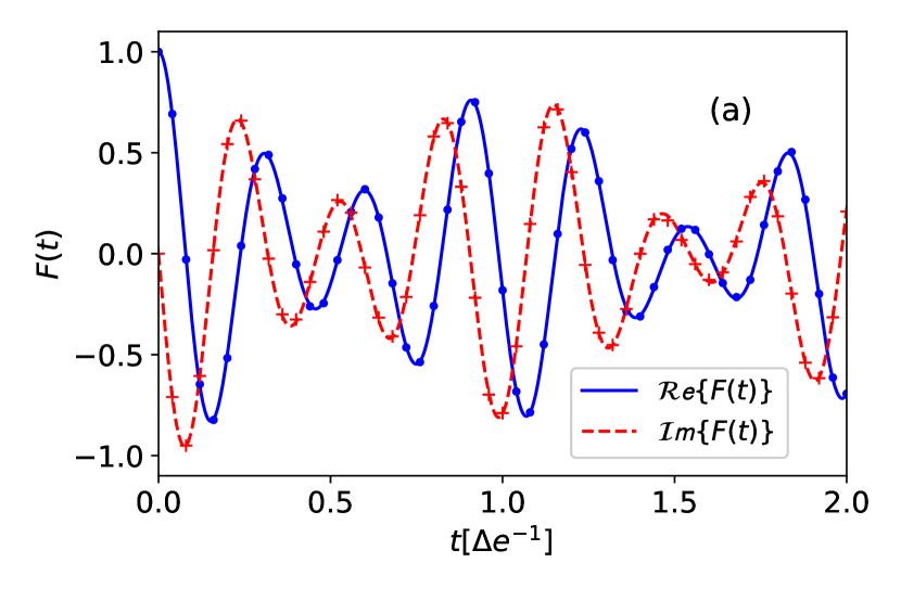
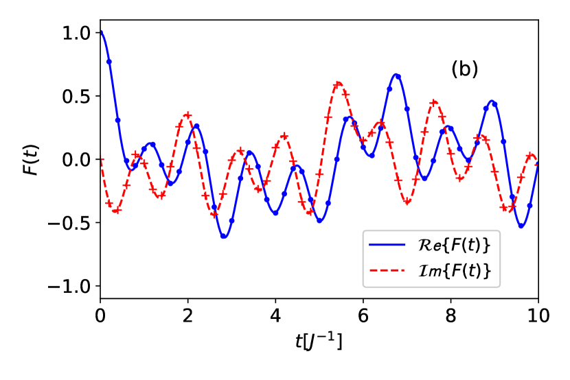
Figure 3: Panel (a): Illustration of the real (blue solid line) and imaginary (red dashed line) parts of the generating function obtained on a classical computer for the pairing model with $N=4$ pairs on $M=8$ doubly degenerated single-particle levels with energy $\varepsilon_{p}=p\Delta e$ (with $p=1,\dots,M$) and $g_{pq}={\rm cte}=g/\Delta e=1$. The initial condition corresponds to the Slater determinants where the 4 lowest single-particle energies are occupied. In panel (b), we show the same quantities obtained for the Fermi-Hubbard model with $N=4$ particles on $M=4$ sites for the parameters $U/J=1$. The initial condition corresponds to a spin-saturated case where the initial state is an average over the $C_{4}^{2}=6$ Slater determinants where pairs of particles with opposite spins occupy randomly 2 sites among the 4 possibilities. Results displayed with symbols in both panels correspond to calculation obtained with the Qiskit-qasm QC software Abr19 and the circuits of Fig. 1. Each point in these figures is obtained by averaging over $10^{4}$ measurements.

II.1.3 Illustration of generating function and Hamiltonian moments obtained by quantum computation

With the use of the Hadamard test and its modified version, together with the different circuits required to perform the time-evolution, we have now all ingredients to extract the real and imaginary part of the generating function $F(t)$ with only one extra ancillary qubit.

We show in Figure 3 the real and imaginary parts of the generating function obtained in the two model cases. The lines correspond to the GF obtained on a classical computer directly by diagonalization of the Hamiltonian. The symbols are the results obtained with the QC simulator using the two circuits shown in Fig. 1. Each points reported in this figure are calculated by averaging $10^{4}$ events using the perfect quantum computer (IBM Qiskit toolkit with qasm Abr19 ). Not surprisingly, since the emulator simulates a perfect QC without noise, the results obtained on the quantum and classical computers perfectly coincide with each other. The only condition is to perform sufficient measurements and to use a numerical time-step $\Delta t$ small enough to insure that the Trotter-Suzuki approximation is valid. We used here $\Delta t.J=0.02$ and $\Delta t.\Delta e=0.002$ for the Fermi-Hubbard and pairing model respectively.

II.2 Physical content of the generating function

The knowledge of the response function at all time gives access to the spectral properties of the Hamiltonian. Indeed, if we introduce a complete set of eigenstates $|\alpha\rangle$ of the Hamiltonian with energy $E_{\alpha}$, we have:

$$F(t)=\sum_{\alpha}e^{-itE_{\alpha}}\langle\alpha|\rho_{0}|\alpha\rangle,=\sum_{\alpha}e^{-itE_{\alpha}}|\langle\alpha|\Phi_{0}\rangle|^{2},$$ (18)

where the last identity holds for a pure initial state $|\Phi_{0}\rangle$. Knowing the generating function for all times gives both the eigenstates energies $E_{\alpha}$ and the amplitudes $|\langle\alpha|\Phi_{0}\rangle|^{2}$. The Fourier transform of the GF, denoted by $\widetilde{F}(\omega)$, also related to the strength or response functions, verifies:

$$\widetilde{F}(\omega) \propto \sum_{\alpha}\delta(\omega-E_{\alpha})|\langle\Phi_{0}|\alpha\rangle|^{2}.$$ (19)

Such response function can be computed directly within the quantum phase-estimation technique Nie02 using a set of ancillary qubits or using only one ancillary qubit as proposed in the present work or in Ref. Som19 .

A second interesting property of the generating function is its connection with the moments, see Eq. (3). For the specific case $\gamma=-it$ and $O=H$, we have the relationship:

$$\langle H^{K}\rangle = i^{K}\left.\frac{d^{K}F(t)}{dt^{K}}\right|_{t=0}.$$ (20)

So that a perfect knowledge of the generating function for all times $t$, gives a priori access to the expectation value of the moments $H^{K}$ calculated for the initial state.

II.3 Critical discussion of the extraction of the moments from the generating function

In the original version of the present article, we proposed to use the finite difference method for the estimate of the left-hand side of Eq. (20). In practice, one could indeed approximately access the different values of $\langle H^{K}\rangle$ by replacing the derivatives by their finite difference expressions (a comprehensive list of finite difference coefficients with various level of accuracy to estimate the derivatives are given for instance in For88 ; Fdi20 ). The finite difference method (FDM) is indeed adequate to obtain rather precise values for the first few moments. This is, for instance, the practical method used in Ref. Ger17 ; Mit18 ; Sch19 to simulate the first derivative of the objective function in the context of quantum machine learning.
The precision on the moments however degrades when the order $K$ increases. Noteworthy, the methods discussed below (Padé or Krylov based) requires rather precise determination of the moments. We have made significant efforts to optimize both the time step and the number of points used in the finite-difference. Our conclusion is that the FDM, even assuming noiseless quantum computers, cannot reach sufficient accuracy to compute $\langle H^{K}\rangle$ as $K$ increases. In the model Hamiltonian considered here, that are relatively simple compare to more realistic Hamiltonians in quantum chemistry or nuclear physics, relatively good accuracy can be achieved with the FDM for moments up to $K=10$ to $15$ depending on the interaction strength. Even if the order of this moments are already quite high, we have observed that a small error on the estimated moments can impact significantly the precision on the post-processing.

Besides the FDM approach, we made extensive tests of polynomial interpolation (standard and Chebyshev) to obtain high precision on the moments. Again, polynomial methods are able to achieve reasonable precision of first moments but are not accurate enough for high $K$ values.

The only approaches that were able to achieve global convergence of all moments with sufficient accuracy are those based on the Fourier transform of the generating function. Indeed, performing the Fourier gives access to approximation of the components of the initial state on the eigenstates, denoted by $p_{\alpha}$, as well as to a set of approximate eigenenergies $\widetilde{E}_{\alpha}$ (see Eq. (19)). Then, from this information, one can simply obtain approximation of $\langle H^{K}\rangle$ using the formula $\sum_{\alpha}\widetilde{E}_{\alpha}^{K}p_{\alpha}$. In the absence of noise on the signal, very good approximation of the moments to any order can be obtained provided that the time-step used is sufficient small to resolve the largest eigen-energy and the time interval $t_{\rm max}$ is sufficiently large to achieve a good energy resolution. The necessity to use Fourier transform requires to compute the generating function for many time steps over rather long time. As a consequence, this significantly increases the effort required to compute the GF on the quantum computer. This aspect, that we seriously underestimated in the first version of this work, render the approach less attractive, especially compared to the quantum-phase-estimation approach that is also based on the Fourier technique.

Despite this difficulty, we give below some illustrations of some possible post-processing assuming that the moments can be computed with good precision.

III Illustration of applications

In this section, we assume that we have obtained a set of moments of the Hamiltonian up to a given, yet limited, order $L$ and illustrate how this information can be used in a second step for post-processing on a classical computer.

III.1 $t$-expansion approach for the ground state energy

As a first illustration, we consider the $t$-expansion technique introduced in Ref. Hor84 and considered more recently in Sek20 in the context of quantum computing. One of the goal of the approach is to obtain the ground state energy denoted by $E_{{\rm GS}}$. In the following, we denoted by $|\Psi_{{\rm GS}}\rangle$ the ground state wave-function.

Given an initial state $|\Phi_{0}\rangle$, our objective is to perform the imaginary-time evolution of this state up to a given time $\tau$, leading to the state

$$|\Psi(\tau)\rangle \equiv \frac{e^{-\tau/2H}}{\sqrt{\langle e^{-\tau H}\rangle}}|\Phi_{0}\rangle.$$

We know that, whatever the initial state $|\Phi_{0}\rangle$, if initially $\langle\Phi_{0}|\Psi_{{\rm GS}}\rangle\neq 0$, then $|\Psi(\tau)\rangle$ will converge to the ground state $|\Psi_{{\rm GS}}\rangle$. We then have:

$$E_{{\rm GS}} = \lim_{\tau\rightarrow\infty}\langle\Psi(\tau)|H|\Psi(\tau)\rangle=\lim_{\tau\rightarrow\infty}E(\tau).$$ (21)

The key aspect underlined in Ref. Hor84 was to show that the convergence of the energy towards the ground state is directly connected to the moments of the Hamiltonian estimated at initial time.

This could be shown by noting that:

$$E(\tau) = \frac{\langle He^{-\tau H}\rangle}{\langle e^{-\tau H}\rangle}=-\frac{d}{d\tau}\ln\langle e^{-\tau H}\rangle,$$ (22)

where the expectation values are taken on the initial state $|\Psi_{0}\rangle$. We recognize in the last expression the generating function $Z(\tau)$ of the cumulants of $H$. More precisely, we have the relationship:

$$Z(\tau) = \ln\langle e^{-\tau H}\rangle=\sum_{K=0}^{+\infty}\frac{(-\tau)^{K}}{K!}\kappa_{K},$$ (23)

where $\kappa_{K}$ is the cumulant of order $K$ of the Hamiltonian that are calculated from the moments of orders lower or equal to $K$ with the initial state. For the sake of completeness, we recall the useful recurrence relation:

$$\kappa_{n} = \langle H^{n}\rangle-\sum_{k=1}^{n-1}\begin{pmatrix}n-1\\ k-1\end{pmatrix}\kappa_{n}\langle H^{n-k}\rangle,$$

that could be used iteratively with the condition $\kappa_{1}=\langle H\rangle$.

Having the set of moments up to a given order informs us on the value of $E(\tau)$ over a certain imaginary time interval $[0,\tau_{max}]$. This interval depends only on the initial state that determines the moment values as well as on the number of available moments.

Figure 4: Illustration of the $t$-expansion method applied to the pairing model. The simulations are performed for the same conditions as panel (a) of Fig. 3. The derivative of the energy and the energy are shown as a function of the imaginary time in panels (a) and (b) respectively. In each panel, the exact (black filled circles), Taylor expansion of Eq. (25) with $M=10$ (blue short-dashed line) and the Padé$[3,7]$ (red long-dashed line) are shown. Note that $M=10$ means that we have used $M+2=12$ cumulants as inputs. The exact imaginary-time solution (black filled circle) was obtained by performing explicitly the imaginary-time evolution on a classical computer. In panel (b), the green horizontal line corresponds to the exact ground state energy.

As was noted in Ref. Hor84 , it might be more efficient to consider the derivative of $E(\tau)$ with respect to $\tau$ than the energy itself to extrapolate the asymptotic value of the energy. Here, we follow closely the prescription proposed in Ref. Hor84 . The evolution of the energy is given by:

$$\frac{d}{d\tau}E(\tau) = -\left(\langle H^{2}\rangle_{\tau}-\langle H\rangle_{\tau}^{2}\right),$$ (24)

where we introduced the notation $\langle.\rangle_{\tau}$ for the expectation values taken at time $\tau$ with $|\Psi(\tau)\rangle$.

Assuming that only the lowest $M+2$ cumulants (or moments) of the Hamiltonian are known, this derivative is approximated as

$$\frac{d}{d\tau}E(\tau) \simeq -\sum_{K=0}^{M}\frac{(-\tau)^{K}}{K!}\kappa_{K+2}.$$ (25)

We then replace this approximate form by a Padé approximation, denoted by Padé$[I,J](\tau)$ where $I$ and $J$ are the orders of the numerator and denominator respectively. The Padé is adjusted such that it reproduces the Taylor expansion given above with the constraint $I+J=M$. The great advantage of using the derivative of the energy stems from the expression (24). Besides the fact that the derivative tends to zero if the Hamiltonian is bound from below, we observe that the energy is always decreasing in imaginary-time evolution. This gives strong constraints on the Padé approximation that could be used. Due to the fact that the derivative, once integrated in time, should give a convergent energy, the decrease of the derivative towards zero should be faster than $1/\tau$. This gives the additional constraint $J-I\geq 2$. Once the Padé approximation that fulfills all these constraints is obtained, the energy $E(\tau)$ is deduced simply by integrating the derivative with respect to $\tau$. We have found that, in the two models considered here, the method is rather accurate to predict the ground state energy $E_{{\rm GS}}$.

We illustrate in Figs. 4 and 5 the $t$-expansion method applied to the two models.

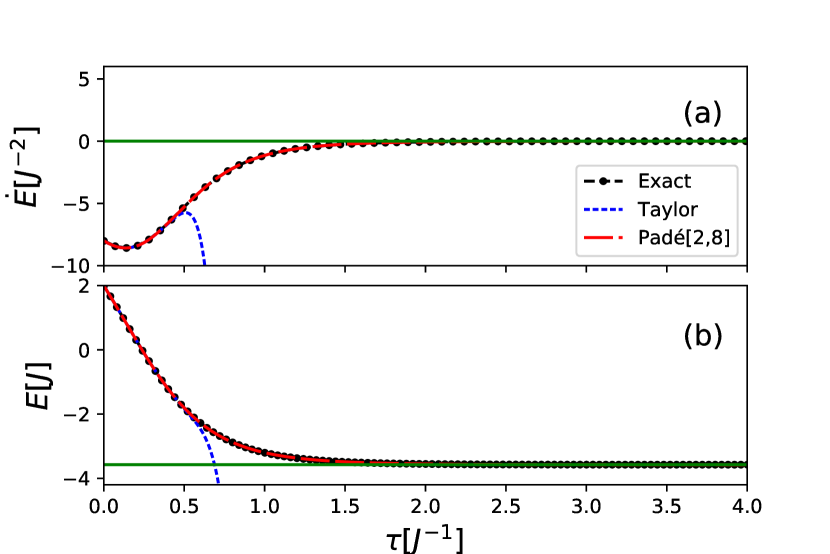
Figure 5: Same as figure Fig. 4 for the Fermi-Hubbard model, with the parameters of Fig. 3. Note that, if only one of the Slater determinants is used instead of the mixing of 6 of them as initial condition, the convergence towards the ground state energy requires to include higher order moments.

We see in both cases that, despite the fact that a finite number of moments are used and that a truncated Taylor expansion (TTE) can only describe the short imaginary-time evolution, the method gives results that are very close to the exact imaginary-time evolution. We clearly see in the TTE in Figs. 4 and 5 that the knowledge of the moments up to a given order only allows us to reproduce the exact evolution of $\dot{E}(\tau)$ and $E(\tau)$ over a certain interval $[0,\tau_{{\rm max}}]$. We show in the illustration here, that the $t$-expansion method can be used to provide rather accurate extrapolation of the system’s ground state energy.

The interval of time over which the TTE is valid depends on the order $M$ of the truncation in Eq. (25). It will also be influenced by the initial state that is used. We illustrate these two aspects for the pairing case in panels (a) and (b) of Fig. 6. In panel (a), the dependence of the convergence of the approach on the number of moments $M+2$ in the inputs is shown (note that the orders $[I,J]$ are changed accordingly to fulfill the constraints $I+J=M$).

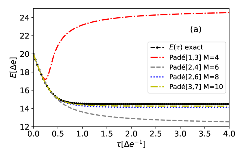
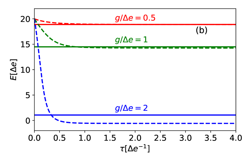
Figure 6: Illustration of the convergence properties of the $t$-expansion for the pairing problem with the same parameters and initial condition as in Fig. 3. In panel (a), results obtained by changing the orders $(I,J)$ in Padé[I,J] are presented. Note that this corresponds to changing the order of truncation $M$ used for the Padé approximation. For comparison, we also show the result of the exact imaginary time evolution (black filled circles) that converges to the exact ground state energy. In Panel (b), the results obtained when $g/\Delta e$ is equal to 0.5 (red), 1.0 (green) and 2.0 (blue) are shown. The dashed lines correspond to the Padé[3,7], Padé[3,7] and Padé[2,8] obtained in all cases with $M=10$ for $g/\Delta e=0.5$, $1.0$ and $2.0$ respectively.

This panel illustrates the rapid convergence of the method when $M$ increases. Note that the $M=4$ case leads to a very bad asymptotic value because the only possibility for the Padé in this case (Padé[1,3]) has a pole leading to a positive unphysical approximation for the derivative of the energy. This problem disappears when $M$ is increased. When $M$ is sufficiently high, there is a flexibility in choosing the order $(I,J)$ even with the constraints given above. We have empirically observed that higher ratios $I/J$ give better results than the case $J-I=2$. Another strong guidance, already noted in Ref. Hor84 , is given by the fact that the Padé approximation of $dE(\tau)/d\tau$ should always be negative.

To illustrate the importance of the initial state on the convergence, we have progressively increased the two-body interaction strength $g$ while keeping the initial state unchanged. When the strength increases, this initial state deviates more and more from the exact ground state. In panel (b) of Fig. 6, we compare the solution of the $t$-expansion approach with a fixed value $M=10$ with the ground state energy. As expected, the predictive power of the method degrades with the increase of $g/\Delta e$. It is still rather encouraging to observe that even for the largest $g$, the result remain reasonably close to the exact solution. Indeed, above $g/\Delta e=1$, the pairing problem becomes highly non-perturbative and a good solution of this problem can only be obtained by using a symmetry breaking state followed by a symmetry restoration Duk04 ; Lac12 ; Deg16 ; Rip17 . We anticipate that the use of initial states obtained using the variation of projections of a $U(1)$ symmetry broken state, like the BCS ansatz, will strongly improve the ground state energy prediction from the $t$-expansion. Work is actually in progress to combine the two techniques on quantum computers. Although we only explore the Padé technique in the present work, we note that the connected moments expansion (CMX) Cio87 can be used as an alternative method to obtain the ground state energy Cla21 ; Pen21 .

III.2 Excited states and time-dependent evolution

Starting from an initial state $|\Phi_{0}\rangle$, the real-time evolution in Hilbert space is given by:

$$|\Phi(t)\rangle = \left(\sum_{K}\frac{(-it)^{K}}{K!}H^{K}\right)|\Phi_{0}\rangle.$$ (26)

We recognize in the expansion the Krylov states denoted by $|\Phi_{K}\rangle\equiv H^{K}|\Phi_{0}\rangle$. In the following, we will consider the Krylov subspace, denoted by ${\cal H}_{M}$, associated to the non-orthogonal basis $\{|\Phi_{0}\rangle,H|\Phi_{0}\rangle,\cdots,H^{M}|\Phi_{0}\rangle\}$. Note that with the present convention, ${\cal H}_{M}$ contains $(M+1)$ states.

The Krylov basis and Krylov subspace is at the heart of several famous algorithms to diagonalize sparse matrices Saa11 . Among the most popular, we mention the Lanczos and the Arnoldi iterative methods that are widely used on classical computers. Quantum equivalents to the Lanczos algorithm have attracted recently special attention Bes20 ; Mot20 ; Bak20 ; Par19 . In a sense, the Krylov basis can be seen as an optimal basis to describe the evolution of a system due to the expansion (26). In the absence of truncation of the Krylov basis, we can describe exactly the evolution for all time. If we now consider the truncated Hilbert space ${\cal H}_{M}$, we will be able to describe exactly the evolution up to the order $t^{M}$ of the expansion.

The expectation values of the initial moments of $H$ contain important information on the Krylov basis. To illustrate the connection between moments and states, let us restrict the evolution of the system in a given subspace ${\cal H}_{M}$. Then, we can write the evolution as:

$$|\Phi(t)\rangle = \sum_{K=0}^{M}c_{K}(t)|\Phi_{K}\rangle,$$ (27)

with the initial condition $|\Phi(0)\rangle=|\Phi_{0}\rangle$.

The approximate evolution in the subspace ${\cal H}_{M}$ is obtained by minimizing the time-dependent variational principle:

$$\delta\int_{0}^{t_{f}}dt\langle\Phi(t)|i\partial_{t}-H|\Phi(t)\rangle dt=0$$ (28)

with respect to all possible variations of the $c_{K}(t)$ or $c_{K}^{*}(t)$. From the variational principle, we deduce the set of time-dependent coupled equations (for all $L$):

$$i\sum_{K}O_{LK}\frac{dc_{K}(t)}{dt} = \sum_{K}H_{LK}c_{K}(t),$$ (29)

with the initial condition $C_{K}(0)=\delta_{K0}$. In this equation, we have defined the matrix elements of the overlap and Hamiltonian matrix:

$$\left\{\begin{array}[]{l}{\displaystyle O_{LK}=\langle\Phi_{L}|\Phi_{K}\rangle=\langle H^{K+L}\rangle_{0},}\\ \\ {\displaystyle H_{LK}=\langle\Phi_{L}|H|\Phi_{K}\rangle=\langle H^{K+L+1}\rangle_{0}}\end{array}\right..$$ (33)

The equations (29) correspond to the standard time-dependent coupled equations (TDCE) that are obtained in a non-orthogonal basis. We see from the definitions (33) that all the ingredients needed to solve these equations are linked to the initial moments of $H$. More precisely, the solution of the TDCE in the subspace ${\cal H}_{M}$ requires the knowledge of the first $L=2M+1$ moments. We show in the appendix A that the use of the variational principle insures that the approximate solution also matches the exact evolution up to order $t^{M}$.

The TDCE can be solved by integrating numerically the time-dependent equations of motion (29). Alternatively, one can transform the problem into an eigenvalue problem in the ${\cal H}_{M}$ subspace, where, for each values of $M$, we generate a set of eigenvalues $E_{\alpha}^{(M)}$ associated to eigenstates denoted by $|\alpha^{(M)}\rangle$. Technically, the solution of the problems is equivalent to an eigenvalue problem in the non-orthogonal basis formed by the states $\{|\Phi_{K}\rangle\}$. This problem is rather standard and can be solved in two steps: (i) first, the overlap matrix given by the $O_{LK}$ in Eq. (33) is diagonalized to obtain a new set of ortho-normal state vectors. The hamiltonian is then diagonalized in the new basis. We illustrate below an application of this techhnique.

III.2.1 Excited states from moments

We show in Fig. 7 the evolution of the $\{E_{\alpha}^{(M)}\}$ values as a function of $M$ for the pairing Hamiltonian case and for the strong coupling regime $g/\Delta e=2.0$.

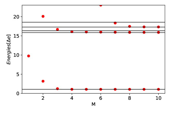
Figure 7: Illustration of the eigenvalues (red filled circles) evolution obtained by the diagonalization of the Hamiltonian in the truncated Krylov basis for increasing $M$ for the pairing model with the same conditions as in Fig. 3 except that the pairing strength is set to $g/\Delta e=2.0$. Note that the number of associated moments used as inputs are given by $L=2M+1$. The horizontal black lines indicate the lowest exact eigenvalues of the pairing Hamiltonian.

In this figure, we see that the energies obtained by diagonalization of the Hamiltonian $H_{M}$ with increasing $M$ converge to some of the exact eigenvalues. The lower is the energy, the faster is the convergence. For the ground state, we observe that a good accuracy is already observed for $M=3$ which corresponds to considering the first 7 moments. In particular, for a number of moments that is lower than the one used in Fig. 4 for $g/\Delta e=1$, a much better accuracy is achieved. Note that in general the dimension of ${\cal H}_{M}$ is rather small compared to the total size of the Hilbert space ($70$ for the pairing model with 4 particles on 8 levels with zero seniority). We systematically observed with the two models that the diagonalization method, compared to the $t$- expansion, not only give access to excited states but also seems to converge more rapidly to the ground state when the number of moments increases. Finally, we note that some excited states are missed due to the fact that their overlaps with the initial state is too low or the Krylov basis size should be further increased. By exploring different initial states, one could expect to obtain the eigenstates that are not reproduced in Fig. 7.

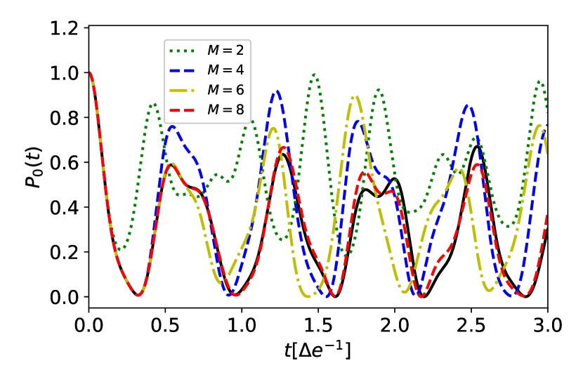
Figure 8: Evolution of the quantity $P_{0}^{(M)}(t)=|\langle\Phi_{0}|\Phi^{(M)}(t)\rangle|^{2}$ as a function of time obtained by solving the TDCE equations with increasing values of $M$ for the pairing model with $g/\Delta e=2$. The black line shows the exact evolution.

III.2.2 Long-time evolution from moments

We now return to one of the main motivations of the present work, i.e. predict the long-time evolution of a quantum complex system. As a follow up of the previous section, we now use the $M$ states obtained by the diagonalization of $H_{M}$. The evolution of the system in the Hilbert space ${\cal H}_{M}$ is given by:

$$|\Phi^{(M)}(t)\rangle = \sum_{\alpha=0}^{M-1}e^{-iE_{\alpha}^{(M)}t}|\alpha^{(M)}\rangle\langle\alpha^{(M)}|\Phi_{0}\rangle.$$ (34)

From this, we can compute the evolution of the survival probability $P_{0}^{(M)}(t)=|\langle\Phi_{0}|\Phi^{(M)}(t)\rangle|^{2}$. Illustrations of the different evolutions of the survival probability obtained with different values of $M$ are shown in Fig. 8 and compared to the exact solution. In all cases, the approximate evolution matches the exact solution up to a certain time $t_{{\rm max}}(M)$. This time increases with $M$. This is expected since the method is designed to give the correct Taylor expansion (26) of the evolution up to order $t^{M}$. We see also that the evolution converges towards the exact solution when $M$ increases even if the number of states included is much lower compared to the size of the complete Hilbert space.

It is worth mentioning that if we now make the Fourier transform of the survival probability to obtain the strength function, already at $M=5$, one would have a good reproduction of several dominant frequencies. This is consistent with Fig. 7 where some of the exact eigenvalues are already well reproduced at rather low $M$ values.

III.3 Application on noisy quantum platforms

As a test, we have tried to compute the generating function on some of the real quantum processor units (QPU) available on the IBM quantum cloud. We focus here on the specific case of the Santiago QPU. Since the number of qubits is limited to 5 in this case, we considered the simple pairing case where a single pair of particles can access two different single-particle levels with spacing $\Delta e$. Such case can be encoded on 2 qubits, plus an extra ancillary qubits to perform the Hadamard or modified Hadamard tests shown in Figs. 1. Raw results obtained with the Santiago QPU turn out to be strongly polluted by noise.

We therefore have tried to implement some standard noise correction techniques. In order to test these error corrections, we have used the FakeSantiago QPU that simulates the topology and the noise of the real Santiago QPU using depolarizing, thermal relaxation and read-out errors. An important aspect to notice is that the implemented circuits on the real and fake Santiago QPU were different compared to the ones shown in Figs. 1. This is because these devices have a set of basic gates which can be implemented and because each device has its own topology. As FakeSantiago emulates the behavior of real Santiago they have the same set of basic gates and topology. The basic gates of FakeSantiago/Santiago did not contain all the gates in the circuits of Figs. 1. Thus the circuits in Figs. 1 had to be replaced by equivalent circuits that use the set of basic gates of each particular device. Also, the new equivalent circuit has to take into account the topology of the device in which is being implemented. The complete process of replacing the theoretical circuits with circuits that we can use in the devices is called transpiling. Qiskit offers several optimizations which can reduce the depth of the transpiled circuits. The results that are shown in Fig. 9 were obtained with a level of optimization of 2 which corresponds to a medium level of optimization. Due to the types of optimizations that this level performs, we can find that different transpilations of the same circuit can generate circuits of different depths. In order to address this, we transpiled the circuit for each point 50 times, and implement the one that had the lower depth. We used the 2^nd level of optimization because we did not find further improvement when using the 3^rd level.

We show in Fig. 9 the evolution of the real and imaginary parts of the generating function obtained with and without the noise. Results without noise correspond to the evolution obtained on a classical computer and on the perfect QC emulator (i.e qasm backend) of Qiskit.

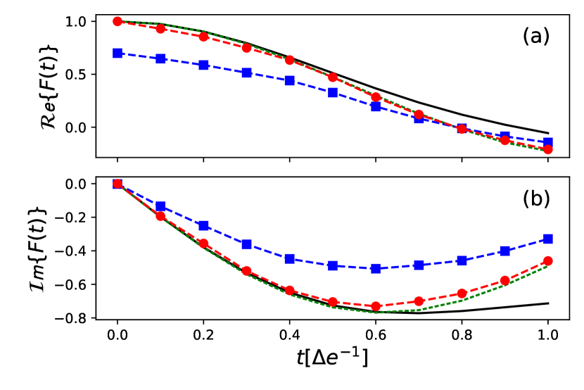
Figure 9: Real (a) and imaginary (b) parts of the generating function obtained for the case of a single pair on two levels with spacing $\Delta e$ and coupling strength $g/\Delta e=1$. The exact result obtained on a classical computer is shown in black solid line. Results obtained with FakeSantiago backend without and with error corrections are shown respectively by blue squares and red circles. We also show for comparison the results obtained with QASM backend (no noise reference quantum calculation) in green long-dashed line. In the quantum simulations, each point is obtained using $10^{6}$ measurements.

We clearly observed in this figure that both real and imaginary parts deviate quite significantly from the exact solution, even at very short time. These deviations stems from two sources (i) the noise that is added in FakeSantiago to simulate the real device and (ii) the discretization of time that was used in the Trotter-Suzuki method. Results obtained in Fig. 9 are calculated by simply assuming a single step in the Trotter-Suzuki technique, i.e. for a given time $t$, the time $\Delta t$ of evolution is directly equal to $t$. This was done in order to minimize the depth of the circuit and thus, the effect of the noise. While for short time $t$, this approximation can be accurate, a single-step in the Trotter approximation will induce deviations from the exact solution when $t$ increases. To illustrate this, we also show in this figure the result obtained with the QASM backend with no noise, same Trotter-Suzuki time-step and same number of measurements. We see that, even in the absence of noise, some deviation with the exact solution occurs when $t$ increases. A simple solution to this problem is to increase the number of steps $n$ in the Trotter-Suzuki methods leading to $t/\Delta t=n$. A drawback is that the depth of the circuit strongly increases when $n$ is increased even by a single unit. This induces a significant increase of the errors on the generating function that could in general not be corrected by the methods discussed below. The results obtained for $n>1$ with error corrections turns out to be worst compared to the case $n=1$.

As an illustration of the effect of error correction, we show in Fig. 9 the results obtained after some specific corrections. To obtain the corrected results, we have used several corrections methods, including the read-out corrections of Ref. Bla04 , supplemented by the post-selection correction correction of Ref. Sun20 . Our aim is not here to make a full description of the error mitigation techniques and readers interested in the technical details can refer to the original articles. These two methods correct partially the noise observed in Fig. 9. To further improve the result, we have also adapted the ”reference correction” technique proposed also in Sun20 . In this approach, we use the fact that we already know the values of the generating function at time $t=0$. With this, we can construct a matrix $M$ that connects the noiseless measurements to the real measurements at this time. It is then assumed that the same matrix $M$ applies at all times. Results obtained using the combination of these three error corrections are shown with red circles in Fig. 9. We see that, with these methods, the error made in the FakeSantiago device can be rather accurately corrected.

We finally mention that we also tried to apply the same protocol with the real Santiago device but the results were more noisy than on the fake device and we were not able to obtain reasonable corrected results. This suggest that, in the NISQ period, the present approach should probably still be combined with variational technique as explored in Ref. Cla21 ; Pen21 .

IV Conclusion

We discuss here the possibility to compute the generating function of an operator using quantum computers, with a focus on the case where the operator is the Hamiltonian itself. The quantum method that we use is based on standard Hadamard tests and is expected to minimize the quantum resources by using a single ancillary qubit. The generating function gives a priori access to the different moments of the operators under interest, that are difficult to compute directly on a quantum computer.
Provided that the moments could be efficiently computed from the calculated generating function, we discuss how this information can be exploited in a post-processing step on a classical computer. We show that the $t$-expansion method in combination with Padé approximation can be used to obtain rather accurate estimates of the ground-state energy. We then illustrate the connection between the moments and the approximate evolution of the system in a truncated Krylov space. The latter approach could be used to study ground state and excited states properties as well as to extrapolate the short-time evolution performed on a quantum computer to an approximation of the long time evolution on a classical computer given that we can approximate with high precision the value of the moments. We note finally the recent Ref. Aul21 , where methods based on moments, including the one discussed here, have been discussed.

One critical aspect to be able to use the generating function as a generator of the moments is definitely the accuracy achieved in computing the different moments. We actually encountered significant difficulties in obtaining the $\langle H^{K}\rangle$ values with high precision when $K$ increases. At present, we have not found a better solution to this problem than performing the Fourier transform/spectral analysis of the time-dependent generating function. Such Fourier transform is rather demanding in terms of quantum resources and, although there is a gain compared to the QPE in terms of circuit length, the numerical effort remains quite significant. After all the tests we made, we believed that the method based on the calculation of moments from the generating function will be rather hard to apply in the NISQ context unless a method, alternative to the Fourier transform and with lower global quantum cost, is found.

Appendix A Validity of the solution in the ${\cal H}_{M}$ space in the TDCE approach

In the present section, we give a direct proof that the use of the TDCE equations (29) in the truncated subspace ${\cal H}_{M}$ insures that the evolution is exact up to order $t^{M}$ in the Taylor series (26). In the following, we will denote by $|\Phi^{(M)}(t)\rangle$ the state obtained by solving the TDCE equation and by $|\Phi(t)\rangle$, the exact solution in the full Hilbert space.

The approximate evolution of the wave-packet associated at a given order $M$ is given by:

$$i\frac{d}{dt}|\Phi^{(M)}(t)\rangle = i\sum_{J=0}^{M}\dot{c}_{J}(t)|\Phi_{J}\rangle.$$

Introducing the inverse of the overlap matrix, we can rewrite this equation as:

$$i\frac{d}{dt}|\Phi^{(M)}(t)\rangle = \sum_{J=0}^{N}|\Phi_{J}\rangle\sum_{KL}O_{JL}^{-1}H_{LK}c_{K}(t)$$ (35)

$$= \sum_{JL}|\Phi_{J}\rangle O_{JL}^{-1}\langle\Phi_{L}|H|\Phi^{(M)}(t)\rangle$$

$$\equiv P_{M}H|\Phi^{(M)}(t)\rangle$$

$$= H_{M}|\Phi^{(M)}(t)\rangle.$$

In the last equation, we have introduced the projector of the Krylov subspace ${\cal H}_{M}$ that is given by:

$$P_{M} = \sum_{I,J=0}^{M}|\Phi_{I}\rangle O_{IJ}^{-1}\langle\Phi_{J}|.$$ (36)

We note in particular that, for all Krylov states with $J\leq M$, we have $P_{M}|\Phi_{I}\rangle=|\Phi_{I}\rangle$. This implies at all time $P_{M}|\Phi^{(M)}(t)\rangle=|\Phi^{(M)}(t)\rangle$. We used this last property to obtain the expression (35), where we have introduced the Hamiltonian projected on ${\cal H}_{M}$, $H_{M}=P_{M}HP_{M}$.

The equation (35) can be formally integrated as:

$$|\Phi^{(M)}(t)\rangle=e^{-itH_{M}}|\Phi_{0}\rangle.$$ (37)

If we now introduce the difference $\Delta_{M}(t)$ between the exact and approximate evolutions, we have:

$$\Delta_{M}(t) \equiv |\Phi(t)\rangle-|\Phi^{(M)}(t)\rangle$$ (38)

$$= \left[e^{-itH}-e^{-itH_{M}}\right]|\Phi_{0}\rangle$$

$$= \sum_{K=0}^{\infty}\frac{(-it)^{K}}{K!}[H^{K}-H_{M}^{K}]|\Phi_{0}\rangle$$

For $K\leq M$, because of the properties of the projector, we have:

$$H_{M}^{K}|\Phi_{0}\rangle = P_{M}H^{K}P_{M}|\Phi_{0}\rangle=P_{M}H^{K}|\Phi_{0}\rangle=P_{M}|\Phi_{K}\rangle$$

$$= |\Phi_{K}\rangle=H^{K}|\Phi_{0}\rangle.$$

Therefore, all terms with $K\leq M$ are strictly zero and the first non-zero term is proportional to $t^{M+1}$.

References

- (1) E. A. Ruiz Guzman and D. Lacroix, Accessing ground state and excited states energies in many-body system after symmetry restoration using quantum computers, in preparation.
- (2) R. P. Feynman, Int. J. Theor. Phys. 21, 467 (1982).
- (3) F. Arute, K. Arya, R. Babbush, D. Bacon, J. C. Bardin, R. Barends, R. Biswas, S. Boixo, F. G. Brandao, D. A. Buell, et al., Nature 574, 505 (2019).
- (4) Y. Alexeev et al, Phys. Rev. X Quantum 2, 017001 (2021)
- (5) J. Preskill, Quantum 2, 79 (2018).
- (6) Suguru Endo, Zhenyu Cai, Simon C. Benjamin, Xiao Yuan, J. Phys. Soc. Jpn., 90, 032001 (2021).
- (7) M. Cerezo et al, Variational Quantum Algorithms, arXiv:2012.09265.
- (8) B. P. Lanyon, J. D. Whitfield, G. G. Gillett, M. E. Goggin, M. P. Almeida, I. Kassal, J. D. Biamonte, M. Mohseni, B. J. Powell, M. Barbieri, et al., Nature chemistry 2, 106 (2010).
- (9) R. Babbush, J. McClean, D. Wecker, A. Aspuru-Guzik, N. Wiebe, Phys. Rev. A 91, 022311 (2015).
- (10) P. J. O’Malley et al., Phys. Rev. X 6, 031007 (2016).
- (11) J. I. Colless, V. V. Ramasesh, D. Dahlen, M. S. Blok, M. E. Kimchi-Schwartz, J. R. McClean, J. Carter, W. A de Jong, and I. Siddiqi, Phys. Rev. X 8, 011021 (2018).
- (12) Cornelius Hempel, Christine Maier, Jonathan Romero, Jarrod McClean, Thomas Monz, Heng Shen, Petar Jurcevic, Ben P. Lanyon, Peter Love, Ryan Babbush, Alán Aspuru-Guzik, Rainer Blatt, and Christian F. Roos Phys. Rev. X 8, 031022 (2018).
- (13) A. Macridin, P. Spentzouris, J. Amundson, R. Harnik, Phys. Rev. Lett. 121, 110504 (2018).
- (14) E.F. Dumitrescu, A.J. McCaskey, G. Hagen, G. R. Jansen, T.D. Morris, T. Papenbrock, R.C. Pooser, D.J. Dean, and P. Lougovski, Phys. Rev. Lett. 120, 210501 (2018).
- (15) Hsuan-Hao Lu, Natalie Klco, Joseph M. Lukens, Titus D. Morris, Aaina Bansal, Andreas Ekström, Gaute Hagen, Thomas Papenbrock, Andrew M. Weiner, Martin J. Savage, and Pavel Lougovski Phys. Rev. A 100, 012320 (2019)
- (16) A. Roggero and J. Carlson, Phys. Rev. C 100, 034610 (2019)
- (17) Weijie Du, James P. Vary, Xingbo Zhao, Wei Zuo, arXiv:2006.01369.
- (18) N. Klco et al., Phys. Rev. A 98, no. 3, 032331 (2018).
- (19) N. Klco and M. J. Savage, Phys. Rev. A 99, 052335 (2019) .
- (20) A. Alexandru et al. , Phys. Rev. Lett. 123, 090501 (2019).
- (21) H. Lamm et al., Phys. Rev. D 100, 034518 (2019).
- (22) Jarrod R McClean et al, Quantum Sci. Technol. 5, 034014 (2020).
- (23) Guido Fano, S. M. Blinder, Mathematical Physics in Theoretical Chemistry, 377 (2019).
- (24) Yudong Cao et al, Chem. Rev. 119, 19, 10856 (2019).
- (25) Sam McArdle, Suguru Endo, Alán Aspuru-Guzik, Simon C. Benjamin, and Xiao Yuan Rev. Mod. Phys. 92, 015003 (2020).
- (26) Bela Bauer, Sergey Bravyi, Mario Motta, Garnet Kin-Lic Chan, arXiv:2001.03685.
- (27) K. Bharti, et. al., arXiv:2101.08448 (2021).
- (28) Emanuel Knill, Gerardo Ortiz, and Rolando D. Somma, Phys. Rev. A 75, 012328 (2007).
- (29) A. Roggero and A. Baroni, Phys. Rev. A 101, 022328 (2020).
- (30) M. A. Nielsen and I. L. Chuang. Quantum information and quantum computation., Cambridge University Press (2000) vol. 2, no 8, p. 23.
- (31) Denis Lacroix, Phys. Rev. Lett. 125, 230502 (2020)
- (32) Bo Peng, Karol Kowalski, Variational quantum solver employing the PDS energy functional, arXiv:2101.08526
- (33) Daniel Claudino, Bo Peng, Nicholas P. Bauman, Karol Kowalski, Travis S. Humble, Improving the accuracy and efficiency of quantum connected moments expansions, Quantum Sci. Technol. 6, 034012 (2021). arXiv:2103.09124
- (34) R. Balian, D. Haar and J. F. Gregg, From Microphysics to Macrophysics: Methods and Applications of Statistical Physics. Volume I and II, Springer Science and Business Media (2007).
- (35) Dominic W. Berry, Andrew M. Childs, Richard Cleve, Robin Kothari, and Rolando D. Somma, Phys. Rev. Lett. 114, 090502 (2015).
- (36) J. D. Hidary, Quantum Computing: An Applied Approach, Springer International Publishing, (2019).
- (37) E. Ovrum. Quantum computing and many-body physics. Master’s thesis, University of Oslo, (2003).
- (38) Ovrum E, Hjorth-Jensen M. Quantum computation algorithm for many-body studies, arXiv:0705.1928v1.
- (39) Rolando D. Somma, New J. Phys. 21, 123025 (2019).
- (40) Alastair Kay, Tutorial on the Quantikz Package, arXiv:1809.03842; DOI: 10.17637/rh.7000520
- (41) P. Jordan and E. Wigner, Zeitschrift fÃŒr Physik 47, 631 (1928).
- (42) Elliott Lieb, Theodore Schultz, Daniel Mattis, Ann. of Phys. 16, 407 (1961).
- (43) R. Somma, G. Ortiz, J. E. Gubernatis, E. Knill, and R. Laflamme Phys. Rev. A 65, 042323 (2002).
- (44) J. T. Seeley, M. J. Richard, and P. J. Love, J. Chem. Phys. 137, 224109 (2012).
- (45) D. Jaksch, C. Bruder, J. I. Cirac, C. W. Gardiner, and P. Zoller, Phys. Rev. Lett. 81, 3108 (1998).
- (46) M. Greiner, O. Mandel, T. Esslinger, T. W. HÀnsch, and I. Bloch, Nature (London) 415, 39 (2002).
- (47) Dave Wecker, Matthew B. Hastings, Nathan Wiebe, Bryan K. Clark, Chetan Nayak, and Matthias Troyer, Phys. Rev. A 92, 062318 (2015)
- (48) Z. Jiang, K. J. Sung, K. Kechedzhi, V. N. Smelyanskiy, and S. Boixo, Phys. Rev. Applied 9, 044036 (2018).
- (49) H. F. Trotter, Proc. Am. Math. Soc. 10, 545 (1959).
- (50) J. von Delft and D. C. Ralf, Phys. Rep. 345, 61 (2001).
- (51) V. Zelevinsky and A. Volya, Phys. of Atomic Nuclei 66, 1781 (2003).
- (52) J. Dukelsky, S. Pittel, and G. Sierra, Rev. Mod. Phys. 76, 643 (2004).
- (53) D. M. Brink and R. A. Broglia, Nuclear Superfluidity: Pairing in Finite Systems (Cambridge University Press, 2005).
- (54) A. Khamoshi, F. A. Evangelista, and G. E. Scuseria, Quantum Sci. Technol. 6, 014004 (2021).
- (55) Héctor Abraham et al [Qiskit collaboration], Qiskit: An Open-source Framework for Quantum Computing, https://qiskit.org/ (2019), DOI: 10.5281/zenodo.2562110
- (56) B. Fornberg, Math. Comp. 51, 699 (1988).
-
(57)
Wiki page for finite difference –
https://en.wikipedia.org/wiki/Finite_difference_coefficient - (58) Gian Giacomo Guerreschi, Mikhail Smelyanskiy, Practical optimization for hybrid quantum-classical algorithms, arXiv:1701.01450.
- (59) Kosuke Mitarai, Makoto Negoro, Masahiro Kitagawa, Keisuke Fujii, Phys. Rev. A 98, 032309 (2018).
- (60) Maria Schuld, Ville Bergholm, Christian Gogolin, Josh Izaac, Nathan Killoran, Phys. Rev. A 99, 032331 (2019).
- (61) Tatiana A. Bespalova, Oleksandr Kyriienko, Hamiltonian operator approximation for energy measurement and ground state preparation , arXiv:2009.03351.
- (62) N.H. Stair, R. Huang, F.A. Evangelista, J. Chem. Theory Comput. 16 2236 (2020) , 16, 2236.
- (63) Kazuhiro Seki, Seiji Yunoki, Phys. Rev. X Quantum 2, 010333 (2021).
- (64) D. Horn and M. Weinstein, Phys. Rev. D 30, 1256 (1984).
- (65) J. Cioslowski, Phys. Rev. Lett. 58, 83 (1987).
- (66) Y. Saad, Numerical Methods for Large Eigenvalue Problems (2nd Edition), Society for Industrial and Applied Mathematic (2011).
- (67) Motta, M., Sun, C., Tan, A.T.K. et al., Nat. Phys. 16, 205 (2020).
- (68) Thomas E. Baker, Phys. Rev. A 103, 032404 (2021).
- (69) R. M. Parrish and P. L. McMahon, Quantum Filter Diagonalization: Quantum Eigendecomposition without Full Quantum Phase Estimation , arXiv:1909.08925 (2019).
- (70) J. Dukelsky, S. Pittel, and G. Sierra, Rev. Mod. Phys. 76, 643 (2004).
- (71) D. Lacroix and D. Gambacurta, Phys. Rev. C 86, 014306 (2012).
- (72) M. Degroote, T. M. Henderson, J. Zhao, J. Dukelsky, and G. E. Scuseria, Phys. Rev. B 93, 125124 (2016).
- (73) J. Ripoche, D. Lacroix, D. Gambacurta, J.-P. Ebran, and T. Duguet Phys. Rev. C 95, 014326 (2017).
- (74) Alexandre Blais, Ren-Shou Huang, Andreas Wallraff, S. M. Girvin, and R. J. Schoelkopf, Phys. Rev. A 69, 062320 (2004).
- (75) Shi-Ning Sun, Mario Motta, Ruslan N. Tazhigulov, Adrian T. K. Tan, Garnet Kin-Lic Chan, Austin J. Minnich, arXiv:2009.03542.
- (76) P. Ring and P. Schuck, The Nuclear Many-Body Problem (Springer-Verlag, New-York, 1980).
- (77) J. P. Blaizot and G. Ripka, Quantum Theory of Finite Systems (MIT Press, Cambridge, 1986).
- (78) L. M. Robledo, , T. R. Rodríguez, and R. R. Rodríguez-Guzmán, Journal of Physics G: Nuclear and Particle Physics 46, 013001 (2018).
- (79) M. Bender, P.-H. Heenen, and P.-G. Reinhard, Rev. Mod. Phys. 75, 121 (2003).
- (80) Joseph C. Aulicino, Trevor Keen, Bo Peng, State preparation and evolution in quantum computing: a perspective from Hamiltonian moments , arXiv:2109.12790.