Altered connectedness of the brain chronnectome during the progression to Alzheimer’s disease

Abstract

Graph theory has been extensively used to investigate brain network topology and its changes in disease cohorts. However, many graph theoretic analysis-based brain network studies focused on the shortest paths or, more generally, cost-efficiency. In this work, we use two new concepts, connectedness and 2-connectedness, to measure different global properties compared to the previously widely adopted ones. We apply them to unravel interesting characteristics in the brain, such as redundancy design and further conduct a time-varying brain functional network analysis for characterizing the progression of Alzheimer’s disease (AD). Specifically, we define different (2-)connectedness states and evaluate their dynamics in AD and its preclinical stage, mild cognitive impairment (MCI), compared to the normal controls (NC). Results indicate that, compared to MCI and NC, brain networks of AD tend to be more frequently connected at a sparse level. For MCI, we found that their brains are more likely to be 2-connected in the minimal connected state as well indicating increasing redundancy in brain connectivity. Such a redundant design could ensure maintained connectedness of the MCI’s brain network in the case that pathological attacks break down any link or silenced any node, making it possible to preserve cognitive abilities. Our study suggests that the redundancy in the brain functional chronnectome could be altered in the preclinical stage of AD. The findings can be successfully replicated in a re-test study and with an independent MCI dataset. Characterizing redundancy design in the brain chronnectome using (2-)connectedness analysis provides a unique viewpoint for understanding disease affected brain networks.

Information Sharing Statement

The source code of the presented method is freely available for use from https://github.com/mghanba/Maryam_Ghanbari_Repository/tree/master.

Declarations

Funding: M.G. was supported by the National Institutes of Health grants (EB022880, AG041721 and AG042599). Z.Z., L.-M.H., P.-T.Y. and D.S. were supported by the National Institutes of Health grant (EB022880). Y.H. and Y.S. were supported by National Natural Science Foundation of China (Grants 61633018, 31371007). H.Z. was supported by the National Institutes of Health grants (EB022880, AG041721, AG049371, and AG042599).
Conflicts of interest/Competing interests: The authors declare that they have no conflict of interest.
Ethics approval: The experiments and data collection were approved by the local ethics committees, as mentioned in ADNI data sharing website http://ad ni.loni.usc.edu. For the Xuanwu hospital’s data, ethical approval has been obtained from the medical research ethics committee and institutional review board of XuanWu Hospital, Capital Medical University (approval number: [2014]011).
Consent to participate: Data used from ADNI is publicly available, so this is not applicable. For the Xuanwu hospital’s data, all participation is based on written informed consent and the participants will be able to withdraw from the study at any time.
Consent for publication: The publisher has the permission from the authors to publish the paper
Availability of data and material: The time series data from all the subjects as well as the calculated redundancy measurements that support our claims are publicly available at https://github.com/mghanba/Maryam_Ghan bari_Repository/tree/master, upon the manuscript is entering review process.
Code availability: The software we used to calculate connectedness and bi-connectedness is SAGE 8.6 (https://www.sagemath.org). The core function for calculating dynamic redundancy statuses and their transitions are publicly available at https://github.com/mghanba/Maryam_Ghanbari_Repository/tree /master, upon the manuscript is entering review process.
Authors’ contributions: H.Z. and D.S. designed and conceptualized the study and revised the manuscript. M.G. drafted and edited the manuscript, analyzed data, interpreted results. H.Z. played a major role in the interpretation of the results and revision of the manuscript. L.-M.H. analyzed the data and revised the manuscript. Z.Z. and P.-T.Y. analyzed data and revised the manuscript. Y.H. and Y.S. collected and analyzed part of the data and revised the manuscript. All authors read and approved the final manuscript.

1 Introduction

The human brain can be modeled as a complex network or graph based on various connectivity metrics, such as functional connectivity (FC, denoting edge weights) that is interpreted as interactions or coordination among different brain regions (denoting nodes) (Sporns 2013). There have been various means to construct brain functional connectome, such as Pearson’s correlation of the resting-state fMRI (rs-fMRI) signals, and it has been recently extended to time-varying (non-stationary or dynamic) connectome, or chronnectome (Chang and Glover 2010; Musso et al. 2010; Sakoğlu et al. 2010; Cribben et al. 2012; Yuan et al. 2012; Hutchison et al. 2013a; Lindquist et al. 2014). The FC or dynamic FC serve as sensitive non-invasive measurements to understand disease-related network alterations. Alzheimer’s Disease (AD) is generally regarded as a disconnection syndrome (Dai et al. 2019) with gradual network topological changes in a prolonged period with a concealed onset (Adeli et al. 2005a, b; Romero-Garcia et al. 2016). Many recent efforts have been put forth to understand the neural underpinning of AD in its early, preclinical stage, also known as mild cognitive impairment (MCI) (Misra et al. 2009; Gauthier et al. 2006; Petersen et al. 2001a; Schwab et al. 2018; Binnewijzend et al. 2012), with brain network modeling using graph theory (Hojjati et al. 2017).

Most complex brain network studies on the AD-related alterations have been largely based on characteristic path length (i.e., the shortest paths) and its derivatives (e.g., assortativity and resilience) (Newman 2006; Ravasz and Barabási 2003; Achard et al. 2006; Newman 2002; Kasthurirathna et al. 2013). For example, the averaged characteristic path length of all pairs of brain regions characterizes network’s global efficiency, while the shortest path-based local connectedness defines local clustering coefficients or local efficiency. Recent studies also broadly defines small-worldness, an important brain network property balancing local integration and global reachability (Stam et al. 2006). AD has been usually associated with disconnected or less efficient connectome with suboptimal organization (Prasad et al. 2015; Supekar et al. 2008; Zippo et al. 2015; Dennis and Thompson 2014). MCI, on the other hand, usually manifests increasing FC and suboptimal small-worldness (Yao et al. 2010, 2018; Zhou et al. 2011), possibly due to a compensatory effect for maintaining normative cognition. While these studies jointly indicated that cost efficiency can be a good property of the brain network where brain regions are optimally connected to work efficiently together, this phenomenon can be also prominent when only network’s backbone (e.g., the top 5% strongest connections) considered (Ma et al. 2018; Latora and Marchiori 2001). The brain network’s topology can manifest different properties when viewed with more redundant (but weaker) links, which could be equally important as the efficiency-based metrics in understanding the neural mechanisms of diseases (Bullmore and Sporns 2009; Wang et al. 2015, 2011).

In this paper, we investigated brain network changes during AD progression by using new brain network topological metrics that are different from the conventional cost-efficiency methods. We did not only rely on the shortest paths (Fig. 1a) but also the less investigated (Di Lanzo et al. 2012), alternative (or parallel, see a toy example in Fig. 1b) paths between each pair of nodes. For example, a magnetoencephalography (MEG)-based FC study defined various redundancy metrics at each frequency band and found that the brain functional network express more redundancy than the random network (Di Lanzo et al. 2012). They further calculated an average number of alternative paths in an electroencephalogram (EEG)-based FC network in the entire network of spinal cord injured patients as a global measurement of redundancy but did not find any significant changes compared to the healthy subjects (Fallani et al. 2011). In an AD vs. control study, education level was found to act as a cognitive reserve by strengthening the redundancy of a partial brain network constructed by using diffusion MRI (Yoo et al. 2015). The inclusion of redundant paths can imply different aspects to the brain connectome, which is further summarized as different types of efficiency, together describing trade-offs among efficiency, cost, and resilience (Avena-Koenigsberger et al. 2018). Different from these previous studies, we proposed an intuitive and easy-to-calculate metric describing whether there are always other paths in addition to the shortest path for every pair of nodes. Such a redundancy design in other natural networks has been consistently found and studied (Corson 2010; Härkegård and Glad 2005; Steiglitz et al. 1969). We hereby analyzed much denser brain networks by also including weak edges, where the backup routes will likely emerge and the redundancy could become the dominant theme compared to cost efficiency.

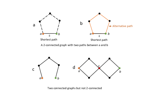
Figure 1: Examples of different connected and 2-connected networks (see main text for details)

Theoretically, a network $G$ with an edge set $E(G)$ and a node set $V(G)$ is connected if there exists a path for any two nodes $a,b\in V(G)$. A connected network $G$ becomes 2-connected if for every node $x\in V(G)$, $G\setminus x$ is connected ($\setminus$ denotes the removal of a node and all the edges adjacent to it). A 2-connected network has better robustness with a merit of the redundancy design (a cycle consisting of any two nodes) compared to the connected network no matter where the attack occurs. By increasing network density, brain network will change from disconnected to connected and to 2-connected. Thus, two critical points may exist during such a transition: the density that a network first becomes connected from disconnected and the density when it transits from connected to 2-connected. 2-connected network has a good property that, if any shortcut is removed, all the regions are still connected (Fig. 1a,b). Of note, if multiple paths exist between $a$ and $b$ but all of them share the same node $c$ (Fig. 1d), they are not redundant paths and the network is not 2-connected. Again, this is not a resilient network because any attack on the node c will break the network. From Fig. 1, it is easy to know that the network (2-)connectedness can provide a sensitive measurement of AD-related changes as a tiny rewiring to the network could dramatically change its (2-)connectedness.

Since AD progression is a spectrum with gradual changes starting from NC converting to MCI, characterizing (2-)connectedness of the brain FC networks at different stages could better help to understand how AD progression impacts the brain. Due to the findings that the brain FC network changes its topology to meet the moment-to-moment requirement for adaptive thinking and other high-order cognitive functions (e.g., attention and alertness) (Damaraju et al. 2014; Demirtaş et al. 2016; Hutchison et al. 2013b; Marusak et al. 2017), we further assumed that the brain could be (2-)connected at different density levels in different period of time. Thus, we analyzed (2-)connectedness and their changes in brain dynamic FC networks. Specifically, we separately assessed connectedness and 2-connectedness of the time-varying FC networks with varied network densities to reveal the aforementioned critical points in a time-resolved manner in NC, MCI, and AD, with specific focuses on both the transitions from disconnected to connected states and those from connected to 2-connected states, and vice versa. Since AD is considered as a disconnected syndrome, we hypothesized that the connectedness status has been altered in AD versus NC and that the brain chronnectome in MCI might generally have more frequently increased redundancy as a compensatory effect to maintain normative cognitive abilities.

2 Methods

2.1 Data

In this study, we apply our method to the Alzheimer’s Disease Neuroimaging Initiative (ADNI) datas (http://adni.loni.usc.edu/). Launched in 2003, the original goal of ADNI was to define imaging biomarkers for use in clinical trials of AD. The current goal has been extended to discover more effective methods to detect AD earlier at its pre-dementia stage. Data quality control was carefully conducted in the ADNI projects to make sure all the data from different imaging centers have the same imaging quality (Jack Jr et al. 2008) (e.g., same imaging protocol, same scanner, and comparable signal-to-noise ratio). The 7-min rs-fMRI data (140 volumes) was preprocessed using AFNI (Cox 1996) according to a standard pipeline (Yan and Zang 2010). Specifically, the first ten volumes are discarded, followed by a rigid-body head motion correction and a nonlinear spatial registration to the Montreal Neurological Institutes (MNI) space. Frame-wise displacement (FD $>0.5$) was considered as excessive head motion and the subjects with more than 2.5-min data (50 volumes) labeled as excessive head motion were discarded (Power et al. 2014). FC was assessed using a functional brain atlas (Shen et al. 2013) consisting of 268 nodes covering the entire brain. Mean rs-fMRI time series of each brain region was band-pass filtered (0.015–0.15 Hz) and further processed to reduce artifacts by regression analysis (nuisance regressors include head motion parameters (the “Friston-24” model), the mean BOLD signal of the white matter, and that of the cerebrospinal fluid).

In the first run of analysis, we compared the dynamic properties of connectedness and 2-connectedness between NC, MCI and AD subjects as a main study to understand how dynamic brain functional network changes its redundancy during AD progression. The subjects were selected from ADNI-Go and ADNI-2 only including the baseline scans and ensuring age ($p$ = 0.752, one-way Analysis of Variance (ANOVA), Table 1) and gender matched among all three groups. Due to the limited sample size of ADs, we selected the same amount of NC and MCI subjects to make sure as many matched data as possible were used.

Table 1: Demographic characteristics (Mean $\pm$ SD) of NC, MCI, AD (used in the main analysis) as well as EMCI and LMCI subjects (also included in the validation analysis)

	Gender (Male/Female)	age (year)	MMSE
NC	49 (26M, 23F)	73.1$\pm$6.5	29.1$\pm$0.9
MCI	49 (26M, 23F)	74.3$\pm$9.8	27.9$\pm$1.6
AD	49 (26M, 23F)	73.3$\pm$8.5	23.1$\pm$2.5
EMCI	49 (26M, 23F)	74.1$\pm$7.6	28.2$\pm$1.8
LMCI	49 (26M, 23F)	72.8$\pm$7.7	26.1$\pm$1.9

2.2 Overview of the dynamic (2-)connectedness analysis

All the analyses were implemented in MATLAB 2017b, SAGE 8.6, Python 2.7, and SPSS 23. Our method includes three parts: 1) calculating dynamic FC networks; 2) assessing connectedness and 2-connectedness at each time window with varied density levels; and 3) comparing dynamic (2-)connectedness among different groups. The flowchart is shown in Fig. 2.

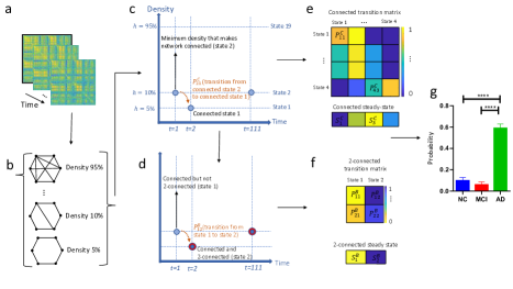
Figure 2: The framework of the dynamic (2-)connectedness analysis. (a) Sliding window correlation-based dynamic FC analysis; (b) Constructing binary networks with different density levels for each sliding window-derived network; (c) Calculating a state vector for time-varying connectedness, where blue points represent connected networks at the minimum density level for every time window; (d) Calculating another state vector for time-varying 2-connectedness by re-visiting the previously detected connected states to check whether they are 2-connected at the same time; (e) and (f) Calculating the transition matrix from the connected and 2-connected state vectors; and (g) Conducting group comparison analysis for each time-varying (2-)connectedness feature among NC, MCI and AD groups

2.3 Dynamic FC network construction

For each subject, a sliding window strategy was used to calculate dynamic FC networks with a window length of 20 volumes (60 s) and a step size of 1 volume (3 s) (Leonardi and Van De Ville 2015). For the BOLD rs-fMRI signals within each window, pairwise Pearson’s correlation was used to calculate brain FC between every pair of the 268 nodes (Fig. 2a). For each of the time-varying FC networks, we calculated its (2-)connected properties at each density level, resulting in a (2-)connectedness property time series for each subject. By definition, connectedness and 2-connectedness are derived from binary networks, where network density is an important parameter that will affect such properties. With a lower density (fewer edges), a network is less likely to be (2-)connected, and vice versa. Searching for a critical point of network density around which the network changes its (2-)connectedness are essential for sensitive group comparisons and for avoiding network saturation at both ends of densities. We applied $H$ different density thresholds to each weighted dynamic FC network to generate $H$ binary networks in each of the $T$ sliding windows (Fig. 2b). In this study, $H$ = 19 (from 5% to 95% with a step size of 5%) and $T$ = 111 (windows).

2.4 Characterizing (2-)connectedness states

Denote these networks by $G_{th}$, $1\leq t\leq T$ and $1\leq h\leq H$. In each window, let $h_{c}$ be the minimum density that makes the corresponding network connected. With $h>h_{c}$, the networks will be all connected with more redundancy; with $h<h_{c}$, the networks are all disconnected. The connectedness and 2-connectedness were assessed at such critical points to avoid trivial results and sensitively detect disease-related alterations. Such critical points can be further regarded as “brain states” in terms of the connectedness (Fig. 2c) and 2-connectedness (Fig. 2d) at a certain period. Denote such a critical network by $G^{*}_{t}$. Like the previous dynamic FC analysis that identifies certain “brain state” for a time window t, we defined a connected state for $G^{*}_{t}$ and assign $h_{c}$ ($1\leq h_{c}\leq H$) as its state label. For example, as shown in Fig. 2c, the network’s connectedness in $t=1$ is in state #2, or $C_{1}=2$. We can created a connected state vector $\textbf{{C}}:=\{C_{t}\}$ ($1\leq t\leq T$) when concatenating the connected states in all time windows, indicating how the dynamic brain network changes its connectedness property. The definition of connected states inherently codes network topology across multiple density settings.

We further checked the $G^{*}_{t}$ to see if it was also 2-connected. If so, we define the network as it is in a 2-connected state #2; if not, state #1. Likewise, we further created a 2-connected state vector $\textbf{{B}}:=\{B_{t}\}$ ($1\leq t\leq T$). For example, $B_{1}$ = 1 (connected but not 2-connected) and $B_{2}$ = 2 (both connected and 2-connected) (Fig. 2d). The state vector B describes how the time-varying brain FC network changes its 2-connected state along time.

There are 19 possible states (since $H$ = 19) for connectedness. However, we found that most transitions among the connected states occurred between #1 to #4; therefore, only the first four connected states were considered in the following analysis. Both of the 2-connected states were used. As the state of 2-connectedness was determined according to the critical point in terms of connectedness, it is irrelevant to a specific network density. Of note, one can define 2-connected states in the same way as that of the connected states; however, since connectedness is a necessary condition for a network to become 2-connected, further checking if the same critical points generates 2-connected network could reveal more sensitive information to subtle changes in the network topology.

2.5 Transition among different (2-)connectedness states

We further quantified the dynamic properties of the connectedness and 2-connectedness states with a transition matrix (describing the probability of one state transitioning to another) and a steady state vector (describing the probability of a certain state be cumulatively occupied given a long enough time, which equals to the normalized “dwelling time”) based on Markov Chain (Williams et al. 2018; Chavez et al. 2010). This resulted in a $4\times 4$ connectedness transition matrix $\textbf{{P}}^{C}:=\{P^{C}_{ij}\}$ (1 $\leq i,j\leq$ 4), where $P^{C}_{ij}$ indicates the probability of changing from state $i$ to $j$, and a $2\times 2$, 2-connectedness transition matrix $\textbf{{P}}^{B}:=\{P^{B}_{ij}\}$ (1 $\leq i,j\leq$ 2). The steady state vector is a probability vector S that satisfies the equation $\textbf{{S.P}}=\textbf{{S}}$, where P is the transition matrix. It was solved as the left eigenvector of P corresponding to the eigenvalue of 1. $\textbf{{S}}^{C}$ and $\textbf{{S}}^{B}$ have a length of four and two, respectively. Therefore, we generated 26 different features, including 16 $P^{C}_{ij}$ in $\textbf{{P}}^{C}$ and $\{S^{C}_{1},S^{C}_{2},S^{C}_{3},S^{C}_{4},P^{B}_{11},P^{B}_{12},P^{B}_{21},P^{B}_{22},S^{B}_{1},S^{B}_{2}\}$ for every subject. Please note that $P^{B}_{11}$ and $P^{B}_{12}$, $P^{B}_{21}$ and $P^{B}_{22}$, as well as $S^{B}_{1}$ and $S^{B}_{2}$ indicate the same features, because $P^{B}_{11}+P^{B}_{12}=1$, $P^{B}_{21}+P^{B}_{22}=1$, and $S^{B}_{1}+S^{B}_{2}=1$. Therefore, only 23 independent features needed to be considered, containing 16 $P^{C}_{ij}$ in $\textbf{{P}}^{C}$ and $\{S^{C}_{1},S^{C}_{2},S^{C}_{3},S^{C}_{4},P^{B}_{11},P^{B}_{12},S^{B}_{1}\}$. However, for completeness, we considered all the 26 features in tables and figures in the following analysis.

2.6 Statistical comparisons among NC, MCI, and AD

For each of the 26 dynamic connectedness features, we conducted a Kruskal-Wallis test (a non-parametric version of the one-way ANOVA) to detect group differences among NC, MCI, and AD groups. Family Wise Error (FWE) corrected $p<$ 0.05 was used to indicate significant group differences. Mann-Withney U-tests (a non-parametric version of the two-sample t-test, two tailed) were further used to conduct post hoc pairwise comparisons for the significant Kruskal-Wallis test results ($p<$ 0.05, FWE corrected).

2.7 Validation with two independent MCI subgroups

To further validate the main results and to see if the revealed abnormalities can be detected at an even earlier stage of MCI, we conducted a second analysis by replacing the MCI group with an independent dataset consisting of two different age- and gender-matched MCI subgroups (early(E-) and late(L-) MCI (Edmonds et al. 2019) selected from the ADNI GO/2 (Table 1). Therefore, we had four different groups (NC, EMCI, LMCI, and AD) that allowed us to further reveal the gradual changes and earlier signs (as shown in the EMCI group) of the AD progression. The NC and AD groups are the same as those in the main analysis. The four groups have comparable age ($p$ = 0.872, one-way ANOVA) and with gender matched. All the data analyses are kept the same as those in the main analysis. The results were compared with the main ones for validation, with a particular focus on whether there were significant differences between NC and EMCI and whether the general results still held from NC to AD.

2.8 Test-retest reliability assessment

We conducted a third analysis by evaluating test-retest reliability of our method and to check if the main findings could be replicated using another follow-up scan from the same subject. Specifically, we identified a follow-up dataset from several of the NC, EMCI, LMCI and AD subjects in Table 1. A total of 14 subjects (7 males and 7 females) from each group have available retest scans and the average test-retest interval for NC, EMCI, LMCI and AD groups are 9.9$\pm$7.6, 7.4$\pm$3.9, 8.8$\pm$3.9 and 4.8$\pm$1.4 months, respectively. Retest samples are age (p = 0.329, one-way ANOVA, two-tailed with degree of freedom 3) and gender matched.

2.9 External validation with independent dataset

In addition to the ADNI dataset, we also used an independent dataset consisting of 67 NC (65.9$\pm$7.2 years old, M/F: 31/36, MMSE = 28$\pm$2.1) and 71 amnestic MCI subjects (68.3$\pm$9.4 years old, M/F: 33/38, MMSE = 24.4$\pm$3.4) and from Xuanwu hospital of Capital Medical University as an out-of-sample validation and reproducibility assessment of our method. The diagnosis of amnestic MCI patients was met the criteria proposed by (Petersen et al. 2001b; Petersen 2004). The details of the data (e.g., inclusion/exclusion criteria, rs-fMRI protocols) were described (Chen et al. 2016). These two groups have comparable age ($p$ = 0.1, 2-sample ttest) and gender ($p$ = 1, chi-square test). This dataset is not included in any centers of ADNI project. The same analysis was conducted comparing the differences in 2-connected steady states ($S_{1}^{B}$ and $S_{2}^{B}$, as the main analysis indicated that MCI tended to have altered 2-connected steady states compared to NCs).

3 Results

3.1 Dynamic brain networks in AD are more likely connected in sparse settings

As shown in Table 2, 10 out of the 26 features had significant group differences as detected by the three-group comparisons based on Kruskal Wallis tests. Post-hoc analysis revealed that the group differences were mainly contributed by AD (i.e., differences were mainly found in AD vs. NC and in AD vs. MCI), except the 2-connected steady states $S^{B}_{1}$ and $S^{B}_{2}$, in which MCI also showed differences from NC (Table 3, Fig. 3).

Table 2: Results from Kruskal-Wallis tests comparing dynamic (2-)connectedness among NC, MCI and AD groups (bold numbers denote significant results after family-wise error corrections)

	$P^{C}_{11}$	$P^{C}_{21}$	$P^{C}_{31}$	$P^{C}_{41}$	$P^{C}_{12}$	$P^{C}_{22}$	$P^{C}_{32}$	$P^{C}_{42}$	$P^{C}_{13}$	$P^{C}_{23}$
NC/MCI/AD	.000	.000	.000	.368	.167	.038	.016	.578	.000	.001

	$P^{C}_{33}$	$P^{C}_{43}$	$P^{C}_{14}$	$P^{C}_{24}$	$P^{C}_{34}$	$P^{C}_{44}$	$S^{C}_{1}$	$S^{C}_{2}$	$S^{C}_{3}$	$S^{C}_{4}$
NC/MCI/AD	.000	.293	.048	.552	.861	.173	.000	.875	.000	.017

	$P^{B}_{11}$	$P^{B}_{12}$	$P^{B}_{21}$	$P^{B}_{22}$	$S^{B}_{1}$	$S^{B}_{2}$
NC/MCI/AD	.892	.892	.991	.991	.000	.000

Table 3: Pairwise comparison results with Mann-Withney U tests on the significant dynamic (2-)connectedness features from Table 2 (bold numbers denote significant results after family-wise error corrections)

	$P^{C}_{11}$	$P^{C}_{21}$	$P^{C}_{31}$	$P^{C}_{13}$	$P^{C}_{23}$	$P^{C}_{33}$	$S^{C}_{1}$	$S^{C}_{3}$	$S^{B}_{1}$	$S^{B}_{2}$
AD/NC	.000	.000	.000	.000	.001	.000	.000	.000	.815	.815
AD/MCI	.000	.000	.000	.000	.002	.000	.000	.000	.000	.000
MCI/NC	.661	.997	.310	.155	.619	.972	.916	.251	.000	.000

For transitions among the connected states, we found that, as long as the connected state #1 (i.e., the brain network is connected at a very sparse setting with only 5% edges) was involved, AD tends to have larger transition probabilities ($P^{C}_{11},P^{C}_{21},P^{C}_{31}$ and $P^{C}_{13}$ , Fig. 3a-d) compared to NC and MCI. These results further led to a more steady connected state #1 in AD ( $S^{C}_{1}$, Fig. 3h). These results indicate that AD tends to spend a longer time with the connected network even under a very sparse setting compared to the other groups. Of note, such results does not mean AD tends to have stronger brain dFC; instead, they altogether mean that the AD’s brain tends to have altered dFC that re-distributed the strongest edges to form a more evenly pattern that made the dynamic network more likely connected. On the other hand, AD subjects have to make big changes in terms of the network density (e.g., change from 5% to 15%, and vice versa, Fig. 3c, d) to maintain connectedness status.

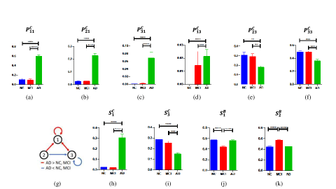
Figure 3: Group comparisons of each dynamic (2-)connected metrics among NC, MCI, and AD groups, where *, **, ***, **** indicate corrected $p$-values at the intervals of (0.01,0.05], (0.001,0.01], (0.0001,0.001], and (0.00001,0.0001], respectively; error bars show standard errors (SE). Subplot (g) summarize major differences between AD and NC/MCI in terms of the transition probabilities of the connectedness states #1-3 (a-f) as well as the steady connected states (h-i)

If the connected state #3 (i.e., the brain network is connected at a not quite sparse setting with 15% edges) was involved and the previous connected states are also not with a quite sparse setting (10% and 15%, rather than 5%), AD tends to have lower $P^{C}_{23}$ and $P^{C}_{33}$, (Fig. 3e, f), possibly due to the dominant findings for $P^{C}_{13}$ and $P^{C}_{31}$. All the results from the connected state transition analysis are summarized in the schematic plot (Fig. 3g).

Different from the fact that AD’s brain network tends to be connected at a low redundancy situation ($h$ = 5%), NC and MCI tend to have connected brain networks in higher redundancy scenarios ($h$ = 15%, Fig. 3i). This indicates that NC and MCI (especially NC) tend to spend more time with the connected network under more redundant network settings compared to AD (possibly due to the strong FCs are more distributed within such functional sub-network, which makes the entire network less likely to be connected in a sparse setting).

3.2 2-connected states could be used to differentiate MCI from NC

When we checked if the network was, at the same time, 2-connected when it first became connected at the critical point, MCI’s brain network showed a more likely tendency to be also 2-connected compared to NC and AD, with the latter two groups showing similar results (Fig. 3k). In other words, at the critical point, MCI’s brain network was less probable to be only connected but not 2-connected compared to NC and AD (Fig. 3j). Of note, both Fig. 3j and Fig. 3k describe the same difference. However, none of the 2-connected state transition $P^{B}_{ij}$ showed any group difference. As the steady 2-connected state showed a significant group difference between NC and MCI, this feature might be adopted to detect AD at its preclinical stage.

3.3 Validation analysis

We successfully validated the main results by replicating the analysis on newly included subdivided MCI groups (EMCI and LMCI). With MCI replaced with two subgroups, the trends among NC, (E/L)MCI, and AD were largely similar (see Online Appendices) compared to the main results in Tables 2 and 3, except $P^{C}_{22}$ and $S^{C}_{4}$ also showed differences among the four groups. The results of EMCI and LMCI were very similar to each other and all together similar (see Online Appendices) to the results of the single MCI group (Fig. 3). Collectively, separating the MCI into EMCI and LMCI did not change the main conclusions.

More interestingly, we spotted a trend (although it was not significant) with continuous changes from EMCI to LMCI and then to AD (see Online Appendices), especially those for $P^{C}_{13}$ and $S^{C}_{3}$ (see Online Appendices). They indicate that there could be gradual changes in terms of the connected state transitions and LMCI subjects are closer to AD than EMCIs. More importantly, as shown in Online Resource the differences in the steady states of 2-connectedness ($S^{B}_{1}$ and $S^{B}_{2}$) between MCI and NC were preserved in the result of EMCI vs. NC, indicating that the detection of potential AD might be achieved at an even earlier (EMCI) stage.

3.4 Test-retest reliability

After repeating the same analysis on the follow-up data from a subset of each of the four groups used in the validation analysis, we found largely similar results (see Online Appendices). As shown in Online Resource, most of the (2-)connectedness features from retest data are similar to the results from the test data. We further plotted the strength of the group differences (as defined by transforming the Kruskal Wallis test-derived $p$-values using $-log(p)$, with a smaller the $p$ indicating a larger group difference) from the test data against those from the retest data. The result indicated an excellent test-retest reliability (with a Spearman correlation $r$ of 0.922) of our method in detection AD-related dynamic network redundancy differences (Fig. 4).

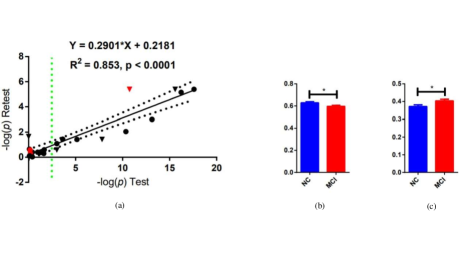
Figure 4: (a) Scatter plot of the four-group comparison results of the 23 (after removing three same dynamic 2-connectedness features, see definitions of 2-connectedness features) dynamic (2-)connectedness features based on the test and retest data where $-log(p)$ quantifies the strength of the group differences. Black and red colors show connected and 2-connected features and round and diamond shapes indicate transition and steady state features, respectively. The green dashed line represents the threshold $p$ = 0.05/23 applied to the test data. (b-c) Comparisons of dynamic 2-connected features, $S^{B}_{1}$ and $S^{B}_{2}$, between NC and amnestic MCI subjects from an independent imaging center (Xuanwu Hospital) for external validation, where * indicates $p<$ 0.05

3.5 External validation with independent dataset

From the main results, we found that NC and MCI showed significant differences in steady 2-connected states $S^{B}_{1}$ and $S^{B}_{2}$. Then we checked these two features on the independent data consisting of NCs and amnestic MCIs from Xuanwu Hospital as an external validation. Since $S^{B}_{2}$ is essentially reflecting the same difference as $S^{B}_{2}$ , only one feature was considered. Therefore, no multiple comparison correction was needed. We found that $S^{B}_{1}$ (and $S^{B}_{2}$) showed a significant difference ($p$ = 0.015, Fig. 4b, c) between NCs and amnestic MCIs, similar to the previous findings between NCs and MCIs based on ADNI datasets (Fig. 3j, k).

4 Discussion

In this paper, we adopted novel brain network attributes, connectedness and 2-connectedness, to quantify dynamic changes in brain chronnectome among different groups at different stages of AD progression. We found that these measurements were able to sensitively detect AD-related topological changes in the spatiotemporal brain functional network patterns. Our major findings are as follows. First, we found that AD subjects had a more frequently connected brain network in the sparse setting (Fig. 3a-c, h). It indicates that AD patients tend to maintain a connected brain network for longer time compared to NC and MCI when only the network backbone is considered. Second, we found that AD subjects manifested large temporal fluctuations in terms of the critical points (e.g., with the minimal network density changing from 5% to 15% to maintain connectedness in consecutive temporal windows, Fig. 3c, d) more frequently than NC and MCI. Third, by considering 2-connectedness, subjects with MCI tend to be also 2-connected more frequently at the critical point of connectedness (Fig. 3j, k). The findings imply that, while the MCI’s brain network (together with the NC’s) tends to become connected with denser edges compared to AD’s, it becomes too complete such that the entire network is more likely to be redundant than AD’s network.

The results jointly indicated gradually altered brain network topology in two folds. On one hand, although AD is generally regarded as a disconnection syndrome (with globally decreased FC compared to NC and MCI), they tend to be more connected in a low density level. This result does not contradict previous findings. This is because the averaged FC weights in AD could be lower than those in NC and MCI, but the strongest FC links in AD could be distributed more evenly from intra- to inter-sub-network connections, making the entire network more likely to be connected. Such a status may not be optimal and stable, as the AD’s brain network can sometimes be quite disconnected and needs more weak connections to be included (a higher density) to maintain connectedness (Fig. 3a-d). On the other hand, when considering 2-connected state with redundant connections, subjects who could be in an early stage of AD (MCI) show more differences compared with NC, where the MCI’s brain network features a more robust and redundant topology (larger probability of steady 2-connected state, Fig. 3k) compared with NC and AD. Such an increment of redundancy may help to ensure a back-up path for every shortest path and maintain the network’s efficiency even under random AD pathological attacks. As such a phenomenon was only detectable in MCIs, it could be interpreted as an overshoot with protective and compensatory effects for MCIs to maintain their cognitive level in the presence of AD-related neurodegeneration (Petersen et al. 2014). More importantly, the MCI’s abnormally elevated redundancy can be detected at an even earlier (i.e., early MCI) stage, indicating good sensitivity of the proposed 2-connectedness measurements.

It is noticeable that the major findings from the multiple ADNI centers are test-retest reliable and reproducible, with an acceptable external validity based on an independent dataset. For example, we found a significant difference between MCI and NC in steady 2-connected state $S^{B}_{1}$ based on the main test (the probabilities for NCs and MCIs are 0.56$\pm$0.10 and 0.44$\pm$0.11), while that from the validation analysis and the retest dataset are very similar (0.56$\pm$0.10 vs. 0.44$\pm$0.08 for NCs and EMCIs, and 0.58$\pm$0.06 vs. 0.38$\pm$0.11 for the retest data from the same NCs and EMCIs). An independent dataset from Xuanwu Hospital revealed the same trend despite an elevated baseline, where the steady 2-connected state $S^{B}_{1}$ from NCs (0.62$\pm$0.08) were still higher than that from amnestic MCIs (0.59$\pm$0.07). The effect size on this difference according to Cohen’s d are large (1.14 for main test, 1.32 for validation analysis, and 2.25 for retest, despite a medium one for the independent test (0.40). The decreased effect size may come from different ethnicities of the subjects from ADNI (mostly Caucasians) and Xuanwu data (all Chinese), different imaging protocols and scanners (e.g., rs-fMRI temporal resolution), different ages and gender ratio (the selected subjects from Xuanwu Hospital are younger than selected ones from ADNI), and/or different MCI diagnostic criteria. Further tests on even larger dataset is necessary to validate our findings.

Graph theory has become a powerful tool in the investigation of brain topological changes in diseased populations including AD (Karwowski et al. 2019). While some previous studies use connectedness as a prerequisite condition to quantify other network attributes (e.g., shortest path length) (Meier et al. 2015), they did not directly compare the connectedness. None of them has ever focused on more redundant network topology such as 2-connectedness. While a handful of previous works have investigated alternative paths (Yoo et al. 2015), none of them examined more stringent (2-)connected properties where all pairs of regions must have one (or more than one) independent paths. Our results suggested that these stringent global properties could be quite sensitive in tracking AD progression. We showed the first-ever evidence that time-varying brain connectedness can be informative to understand AD progression. While the majority of the complex brain network studies focused on the shortest pathsregions (Meier et al. 2015) and the derived metrics (e.g., betweenness centrality (Rubinov and Sporns 2010) and connector hub (van den Heuvel and Sporns 2013), we showed that other lengthier pathways could be also informative, thanks to the similar concepts and applications in the other fields (Corson 2010; Härkegård and Glad 2005; Steiglitz et al. 1969; White and Newman 2001; Quattrociocchi et al. 2014). To further increase sensitivity, we extend such a concept to dynamic FC network by investigating how the brain changes its reserved paths in a time-varying manner, making it feasible to detect subtle changes in a diseased condition. The framework can be easily applied to other brain diseases and mental disorders.

While the current framework focused on dynamic networks, it is straightforward to apply it to static brain network or a structural connectivity network based on diffusion MRI. In addition, 2-connectedness can be further extended to 3-connectedness (at least three independent paths exist for every pair of brain regions) for network studies in a more redundant scenario. The current work characterized the entire brain network; to improve spatial specificity, one can investigate functional sub-networks (e.g., default mode network) or a sub-network associated with each region for a fine-grained investigation and biomarker detection.

In conclusion, we used novel network redundancy measurements to reveal how dynamic brain functional network changes its topology in more denser conditions during the AD progression. The reliable and reproducible findings provide a new view angle to the AD-related brain networks and a sensitive means to detect AD in its early stage. We advocate that the redundant design is as important as cost efficiency and could be promising for the future network neuroscience studies.

References

- Achard et al. (2006) Achard S, Salvador R, Whitcher B, Suckling J, Bullmore E (2006) A resilient, low-frequency, small-world human brain functional network with highly connected association cortical hubs. Journal of Neurosci 26(1):63–72
- Adeli et al. (2005a) Adeli H, Ghosh-Dastidar S, Dadmehr N (2005a) Alzheimer’s disease and models of computation: Imaging, classification, and neural models. Journal of Alzheimer’s Disease 7(3):187–199
- Adeli et al. (2005b) Adeli H, Ghosh-Dastidar S, Dadmehr N (2005b) Alzheimer’s disease: models of computation and analysis of EEGs. Clinical EEG and Neurosci 36(3):131–140
- Avena-Koenigsberger et al. (2018) Avena-Koenigsberger A, Misic B, Sporns O (2018) Communication dynamics in complex brain networks. Nature Reviews Neuroscience 19(1):17
- Binnewijzend et al. (2012) Binnewijzend MA, Schoonheim MM, Sanz-Arigita E, Wink AM, van der Flier WM, Tolboom N, Adriaanse SM, Damoiseaux JS, Scheltens P, van Berckel BN, et al. (2012) Resting-state fMRI changes in alzheimer’s disease and mild cognitive impairment. Neurobiology of Aging 33(9):2018–2028
- Bullmore and Sporns (2009) Bullmore E, Sporns O (2009) Complex brain networks: graph theoretical analysis of structural and functional systems. Nature Reviews Neurosci 10(3):186
- Chang and Glover (2010) Chang C, Glover GH (2010) Time-frequency dynamics of resting-state brain connectivity measured with fMRI. NeuroImage 50(1):81–98
- Chavez et al. (2010) Chavez M, Valencia M, Latora V, Martinerie J (2010) Complex networks: new trends for the analysis of brain connectivity. International J of Bifurcation and Chaos 20(06):1677–1686
- Chen et al. (2016) Chen GQ, Sheng C, Li YX, Yu Y, Wang XN, Sun Y, Li HY, Li XY, Xie YY, Han Y (2016) Neuroimaging basis in the conversion of aMCI patients with apoe-4 to ad: study protocol of a prospective diagnostic trial. BMC neurology 16(1):64
- Corson (2010) Corson F (2010) Fluctuations and redundancy in optimal transport networks. Physical Review Letters 104(4):048703
- Cox (1996) Cox RW (1996) AFNI : software for analysis and visualization of functional magnetic resonance neuroimages. Computers and Biomedical Research 29(3):162–173
- Cribben et al. (2012) Cribben I, Haraldsdottir R, Atlas LY, Wager TD, Lindquist MA (2012) Dynamic connectivity regression: determining state-related changes in brain connectivity. NeuroImage 61(4):907–920
- Dai et al. (2019) Dai Z, Lin Q, Li T, Wang X, Yuan H, Yu X, He Y, Wang H (2019) Disrupted structural and functional brain networks in alzheimer’s disease. Neurobiology of Aging 75:71–82
- Damaraju et al. (2014) Damaraju E, Allen EA, Belger A, Ford JM, McEwen S, Mathalon D, Mueller B, Pearlson G, Potkin S, Preda A, et al. (2014) Dynamic functional connectivity analysis reveals transient states of dysconnectivity in schizophrenia. NeuroImage: Clinical 5:298–308
- Demirtaş et al. (2016) Demirtaş M, Tornador C, Falcon C, López-Solà M, Hernández-Ribas R, Pujol J, Menchon JM, Ritter P, Cardoner N, Soriano-Mas C, et al. (2016) Dynamic functional connectivity reveals altered variability in functional connectivity among patients with major depressive disorder. Human Brain Mapping 37(8):2918–2930
- Dennis and Thompson (2014) Dennis EL, Thompson PM (2014) Functional brain connectivity using fMRI in aging and alzheimer’s disease. Neuropsychology Review 24(1):49–62
- Di Lanzo et al. (2012) Di Lanzo C, Marzetti L, Zappasodi F, De Vico Fallani F, Pizzella V (2012) Redundancy as a graph-based index of frequency specific meg functional connectivity. Computational and mathematical methods in medicine 2012
- Edmonds et al. (2019) Edmonds EC, McDonald CR, Marshall A, Thomas KR, Eppig J, Weigand AJ, Delano-Wood L, Galasko DR, Salmon DP, Bondi MW, et al. (2019) Early versus late MCI : Improved MCI staging using a neuropsychological approach. Alzheim & Dem 15(5):699–708
- Fallani et al. (2011) Fallani FDV, Rodrigues FA, da Fontoura Costa L, Astolfi L, Cincotti F, Mattia D, Salinari S, Babiloni F (2011) Multiple pathways analysis of brain functional networks from EEG signals: an application to real data. Brain topography 23(4):344–354
- Gauthier et al. (2006) Gauthier S, Reisberg B, Zaudig M, Petersen RC, Ritchie K, Broich K, Belleville S, Brodaty H, Bennett D, Chertkow H, et al. (2006) Mild cognitive impairment. The Lancet 367(9518):1262–1270
- Härkegård and Glad (2005) Härkegård O, Glad ST (2005) Resolving actuator redundancy—optimal control vs. control allocation. Automatica 41(1):137–144
- van den Heuvel and Sporns (2013) van den Heuvel MP, Sporns O (2013) Network hubs in the human brain. Trends in Cognitive Sciences 17(12):683–696
- Hojjati et al. (2017) Hojjati SH, Ebrahimzadeh A, Khazaee A, Babajani-Feremi A, Initiative ADN, et al. (2017) Predicting conversion from MCI to AD using resting-state fMRI, graph theoretical approach and SVM. Journal of Neurosci Methods 282:69–80
- Hutchison et al. (2013a) Hutchison RM, Womelsdorf T, Allen EA, Bandettini PA, Calhoun VD, Corbetta M, Della Penna S, Duyn JH, Glover GH, Gonzalez-Castillo J, et al. (2013a) Dynamic functional connectivity: promise, issues, and interpretations. NeuroImage 80:360–378
- Hutchison et al. (2013b) Hutchison RM, Womelsdorf T, Allen EA, Bandettini PA, Calhoun VD, Corbetta M, Della Penna S, Duyn JH, Glover GH, Gonzalez-Castillo J, et al. (2013b) Dynamic functional connectivity: promise, issues, and interpretations. NeuroImage 80:360–378
- Jack Jr et al. (2008) Jack Jr CR, Bernstein MA, Fox NC, Thompson P, Alexander G, Harvey D, Borowski B, Britson PJ, L Whitwell J, Ward C, et al. (2008) The alzheimer’s disease neuroimaging initiative (ADNI ): MRI methods. Journal of Magnetic Resonance Imaging: An Official Journal of the International Society for Magnetic Resonance in Medicine 27(4):685–691
- Karwowski et al. (2019) Karwowski W, Vasheghani Farahani F, Lighthall N (2019) Application of graph theory for identifying connectivity patterns in human brain networks: A systematic review. Frontiers in Neurosci 13:585
- Kasthurirathna et al. (2013) Kasthurirathna D, Piraveenan M, Thedchanamoorthy G (2013) On the influence of topological characteristics on robustness of complex networks. Journal of Artificial Intelligence and Soft Computing Research 3(2):89–100
- Latora and Marchiori (2001) Latora V, Marchiori M (2001) Efficient behavior of small-world networks. Physical Review Letters 87(19):198701
- Leonardi and Van De Ville (2015) Leonardi N, Van De Ville D (2015) On spurious and real fluctuations of dynamic functional connectivity during rest. NeuroImage 104:430–436
- Lindquist et al. (2014) Lindquist MA, Xu Y, Nebel MB, Caffo BS (2014) Evaluating dynamic bivariate correlations in resting-state fMRI: a comparison study and a new approach. NeuroImage 101:531–546
- Ma et al. (2018) Ma X, Jiang G, Fu S, Fang J, Wu Y, Liu M, Xu G, Wang T (2018) Enhanced network efficiency of functional brain networks in primary insomnia patients. Frontiers in Psychiatry 9:46
- Marusak et al. (2017) Marusak HA, Calhoun VD, Brown S, Crespo LM, Sala-Hamrick K, Gotlib IH, Thomason ME (2017) Dynamic functional connectivity of neurocognitive networks in children. Human Brain Mapping 38(1):97–108
- Meier et al. (2015) Meier J, Tewarie P, Van Mieghem P (2015) The union of shortest path trees of functional brain networks. Brain Connectivity 5(9):575–581
- Misra et al. (2009) Misra C, Fan Y, Davatzikos C (2009) Baseline and longitudinal patterns of brain atrophy in MCI patients, and their use in prediction of short-term conversion to ad: results from ADNI. NeuroImage 44(4):1415–1422
- Musso et al. (2010) Musso F, Brinkmeyer J, Mobascher A, Warbrick T, Winterer G (2010) Spontaneous brain activity and EEG microstates. a novel EEG/fMRI analysis approach to explore resting-state networks. NeuroImage 52(4):1149–1161
- Newman (2002) Newman ME (2002) Assortative mixing in networks. Physical Review Letters 89(20):208701
- Newman (2006) Newman ME (2006) Modularity and community structure in networks. Proceedings of the National Academy of Sciences 103(23):8577–8582
- Petersen (2004) Petersen RC (2004) Mild cognitive impairment as a diagnostic entity. Journal of internal medicine 256(3):183–194
- Petersen et al. (2001a) Petersen RC, Doody R, Kurz A, Mohs RC, Morris JC, Rabins PV, Ritchie K, Rossor M, Thal L, Winblad B (2001a) Current concepts in mild cognitive impairment. Archives of Neurol 58(12):1985–1992
- Petersen et al. (2001b) Petersen RC, Doody R, Kurz A, Mohs RC, Morris JC, Rabins PV, Ritchie K, Rossor M, Thal L, Winblad B (2001b) Current concepts in mild cognitive impairment. Archives of neurology 58(12):1985–1992
- Petersen et al. (2014) Petersen RC, Caracciolo B, Brayne C, Gauthier S, Jelic V, Fratiglioni L (2014) Mild cognitive impairment: a concept in evolution. Journal of Internal Medicine 275(3):214–228
- Power et al. (2014) Power JD, Mitra A, Laumann TO, Snyder AZ, Schlaggar BL, Petersen SE (2014) Methods to detect, characterize, and remove motion artifact in resting state fMRI. NeuroImage 84:320–341
- Prasad et al. (2015) Prasad G, Joshi SH, Nir TM, Toga AW, Thompson PM, ADNI, et al. (2015) Brain connectivity and novel network measures for alzheimer’s disease classification. Neurobiology of Aging 36:S121–S131
- Quattrociocchi et al. (2014) Quattrociocchi W, Caldarelli G, Scala A (2014) Self-healing networks: redundancy and structure. PLoS one 9(2)
- Ravasz and Barabási (2003) Ravasz E, Barabási AL (2003) Hierarchical organization in complex networks. Physical Review E 67(2):026112
- Romero-Garcia et al. (2016) Romero-Garcia R, Atienza M, Cantero JL (2016) Different scales of cortical organization are selectively targeted in the progression to alzheimer’s disease. International J of Neural Systems 26(02):1650003
- Rubinov and Sporns (2010) Rubinov M, Sporns O (2010) Complex network measures of brain connectivity: uses and interpretations. NeuroImage 52(3):1059–1069
- Sakoğlu et al. (2010) Sakoğlu Ü, Pearlson GD, Kiehl KA, Wang YM, Michael AM, Calhoun VD (2010) A method for evaluating dynamic functional network connectivity and task-modulation: application to schizophrenia. Magnetic Resonance Materials in Physics, Biology and Medicine 23(5-6):351–366
- Schwab et al. (2018) Schwab S, Afyouni S, Chen Y, Han Z, Guo Q, Dierks T, Wahlund LO, Grieder M (2018) Functional connectivity alterations of the temporal lobe and hippocampus in semantic dementia and alzheimer’s disease. BioRxiv p 322131
- Shen et al. (2013) Shen X, Tokoglu F, Papademetris X, Constable RT (2013) Groupwise whole-brain parcellation from resting-state fMRI data for network node identification. NeuroImage 82:403–415
- Sporns (2013) Sporns O (2013) Structure and function of complex brain networks. Dialogues Clin Neurosci 15(3):247
- Stam et al. (2006) Stam CJ, Jones B, Nolte G, Breakspear M, Scheltens P (2006) Small-world networks and functional connectivity in alzheimer’s disease. Cerebral Cortex 17(1):92–99
- Steiglitz et al. (1969) Steiglitz K, Weiner P, Kleitman D (1969) The design of minimum-cost survivable networks. IEEE Transactions on Circuit Theory 16(4):455–460
- Supekar et al. (2008) Supekar K, Menon V, Rubin D, Musen M, Greicius MD (2008) Network analysis of intrinsic functional brain connectivity in alzheimer’s disease. PLoS Computational Biology 4(6):e1000100
- Wang et al. (2015) Wang J, Wang X, Xia M, Liao X, Evans A, He Y (2015) Gretna: a graph theoretical network analysis toolbox for imaging connectomics. Frontiers in Human Neurosci 9:386
- Wang et al. (2011) Wang JH, Zuo XN, Gohel S, Milham MP, Biswal BB, He Y (2011) Graph theoretical analysis of functional brain networks: test-retest evaluation on short-and long-term resting-state functional MRI data. PloS one 6(7)
- White and Newman (2001) White DR, Newman M (2001) Fast approximation algorithms for finding node-independent paths in networks. Santa Fe Institute Working Papers Series
- Williams et al. (2018) Williams NJ, Daly I, Nasuto S (2018) Markov model-based method to analyse time-varying networks in EEG task-related data. Frontiers in Computational Neuroscience 12:76
- Yan and Zang (2010) Yan C, Zang Y (2010) DPARSF: a MATLAB toolbox for” pipeline” data analysis of resting-state fMRI. Frontiers in systems Neurosci 4:13
- Yao et al. (2010) Yao Z, Zhang Y, Lin L, Zhou Y, Xu C, Jiang T, ADNI, et al. (2010) Abnormal cortical networks in mild cognitive impairment and alzheimer’s disease. PLoS Computational Biology 6(11):e1001006
- Yao et al. (2018) Yao Z, Hu B, Chen X, Xie Y, Gutknecht J, Majoe D (2018) Learning metabolic brain networks in MCI and AD by robustness and leave-one-out analysis: An FDG-PET study. American Journal of Alzheimer’s Disease & Other Dementias 33(1):42–54
- Yoo et al. (2015) Yoo SW, Han CE, Shin JS, Seo SW, Na DL, Kaiser M, Jeong Y, Seong JK (2015) A network flow-based analysis of cognitive reserve in normal ageing and alzheimer’s disease. Scientific reports 5:10057
- Yuan et al. (2012) Yuan H, Zotev V, Phillips R, Drevets WC, Bodurka J (2012) Spatiotemporal dynamics of the brain at rest—exploring EEG microstates as electrophysiological signatures of bold resting state networks. NeuroImage 60(4):2062–2072
- Zhou et al. (2011) Zhou Y, Ge Y, Dougherty J (2011) Small world network properties changes in mild cognitive impairment and early alzheimer’s disease. Alzheim & Dem: The Journal of the Alzheimer’s Association 7(4):S729
- Zippo et al. (2015) Zippo AG, Castiglioni I, Borsa VM, Biella GE (2015) The compression flow as a measure to estimate the brain connectivity changes in resting state fMRI and 18FDG-PET alzheimer’s disease connectomes. Frontiers in Computational Neurosci 9:148