Transparent Electricity Pricing with Privacy

Abstract

Smart grids leverage data from smart meters to improve operations management and to achieve cost reductions. The fine-grained meter data also enable pricing schemes that simultaneously benefit electricity retailers and users. Our goal is to design a practical dynamic pricing protocol for smart grids in which the rate charged by a retailer depends on the total demand among its users. Realizing this goal is challenging because neither the retailer nor the users are trusted. The first challenge is to design a pricing scheme that incentivizes consumption behavior that leads to lower costs for both the users and the retailer. The second challenge is to prevent the retailer from tampering with the data, for example, by claiming that the total consumption is much higher than its real value. The third challenge is data privacy, that is, how to hide the meter data from adversarial users. To address these challenges, we propose a scheme in which peak rates are charged if either the total or the individual consumptions exceed some thresholds. We formally define a privacy-preserving transparent pricing scheme (PPTP) that allows honest users to detect tampering at the retailer while ensuring data privacy. We present two instantiations of PPTP, and prove their security. Both protocols use secure commitments and zero-knowledge proofs. We implement and evaluate the protocols on server and edge hardware, demonstrating that PPTP has practical performance at scale.

1 Introduction

Smart meters, the building blocks of smart grids, allow electricity retailers to measure their customers’ power use at a frequency that is far beyond the capabilities of traditional meters, which rely on sporadic manual readouts. One important use case for a higher data frequency is that it enables more accurate and informative bills. The high measurement frequency also enables advanced electricity pricing. Since the retailer’s costs are highest during periods of high network demand, it is often profitable to incentivize users to spread their demand across the day by charging them different rates during peak and off-peak periods. This is ultimately also beneficial for the customers themselves because a retailer with lower costs can offer more competitive prices.

Pricing schemes that are based on fixed peak and off-peak rates do not make full use of the smart meter’s potential, which includes the ability to receive up-to-date pricing information that reflects network conditions observed by the retailer. To improve on this, dynamic pricing schemes [14] allow the retailer to anticipate periods of high electricity demand, e.g., heatwaves or major sporting events, and incentivize users to shift their loads away from these periods. In this set-up, the retailer shares pricing information with the meters at the start of each operational cycle (e.g., at midnight), which can then be forwarded to a smart home hub that coordinates high-demand activities (e.g., charging an electric vehicle) across the household. In return, the meter periodically sends measurements back to the retailer, and after a number of operational cycles – an operational cycle typically lasts a single day – the user is presented with an electricity bill that reflects the power usage and prices throughout the cycles. However, prior research [2, 14] has found that users are uncomfortable with pricing schemes that they perceive to be overly complex or risky.

Our goal is to design a practical dynamic pricing protocol. This is challenging because neither the retailers nor the users are trusted. In particular, the first challenge is to design a pricing scheme that can simultaneously reduce the costs of the retailer and the users – i.e., that the retailer is able to charge higher prices during periods when the actual demand is high across the network. The second challenge is to prevent the retailer from giving wrong information about network-level demand – i.e., that it cannot tamper with the aggregate measurements from the meters. The third challenge is to share network-level information without revealing the users’ privacy-sensitive measurements to other users – i.e., that an honest-but-curious user cannot learn other users’ measurements.

The latter two challenges have been studied in the related literature, e.g., by Shi et al. [13] and others [1, 6]. However, these works use a different threat model than the one that is most relevant in our setting. For example, in the work by Shi et al. [13] the retailer is not trusted with knowledge of individual users’ measurements. Since the retailer in our model needs the measurements anyway to compute the bills, we can afford a more relaxed trust assumption, namely that the privacy requirement only applies to honest-but-curious users. Another difference is that Shi et al. [13] do not consider strict integrity of the aggregate data – therefore, in their setting random noise can be added to measurements, but allowing this in our setting would mean that the retailer can increase its profits by inflating the aggregate value. In summary, our threat model gives us opportunities to design a more efficient privacy-preserving protocol, while at the same time necessitating the protection of measurement integrity.

To address the above challenges, we present a privacy-preserving and transparent pricing (PPTP) scheme. The scheme addresses the first challenge by charging a peak or off-peak rate depending on the actual network demand. This protects the retailer from the risk of financial losses during a demand surge while being fully transparent to the user. It is predictable for the user as network demand under normal circumstances can be predicted with reasonable accuracy given historical data [9]. To address the second challenge, we require the retailer to share verifiable proofs about users’ measurements. To address the third challenge, we use zero-knowledge range proofs that do not reveal the underlying measurements, e.g., Bulletproofs [4]. We formalize the security definition of PPTP and present two instantiations: a baseline protocol that shares the full set of range proofs with each user, and a more efficient one that uses Merkle trees and which uses concepts from related work on Certificate Transparency [5, 7]. We prove the security of both instantiations, and evaluate their performance on a server and on edge devices. The results show that PPTP achieves practical performance at scale.

In summary, we make the following contributions.

1. We present a dynamic pricing protocol for smart grids that reduces the cost for both the retailer and users.

2. We define a privacy-preserving and transparent pricing (PPTP) scheme that ensures integrity of the retailer when computing dynamic prices. PPTP protects confidentiality of the meter data against malicious users.

3. We instantiate two PPTP protocols and prove their security properties.

4. We implement the two protocols and demonstrate their performance at scale using a server and Raspberry Pi hardware.

Throughout this paper, we use the notation $[k]$ to denote $\{1,\ldots,k\}$ for $k\in\mathbb{N}$. A summary of the other notation used in the paper can be found in Table 1. The structure of the paper is as follows. In Section 2, we present our model of the system’s cost and price structure. The network model, threat model, and requirements are presented in Section 3. The two PPTP instantiations are presented in Sections 4 and 5. We present the experimental results in Section 6 and discuss related work in Section 7. Section 8 concludes the paper.

Table 1: Summary of the notation used in this paper.

symbol		values		meaning
$n$		$\mathbb{N}$		number of users
$k$		$\mathbb{N}$		number of time periods per operational cycle
$p_{i\,t}$		$\mathbb{N}$		rate charged to user $i\in[n]$ in period $t\in[k]$
$B_{i}$		$\mathbb{N}$		bill of user $i\in[n]$
$\alpha_{t}$		$\mathbb{N}$		peak rate in period $t\in[k]$
$\beta_{t}$		$\{0,\ldots,\alpha_{t}\}$		off-peak rate in period $t\in[k]$
$\gamma_{t}$		$\{0,n\delta_{t}-1\}$		system peak rate threshold in period $t\in[k]$
$\delta_{t}$		$\mathbb{N}$		individual peak rate threshold in period $t\in[k]$
$y_{i\,t}$		$\mathbb{N}$		raw measurement of user $i\in[n]$ in period $t\in[k]$
$x_{i\,t}$		$\{0,\delta_{t}\}$		truncated measurement of user $i\in[n]$ in period $t\in[k]$
$r_{i\,t}$		$\mathcal{R}_{\text{c}}$		random secret of user $i\in[n]$ in period $t\in[k]$
$c_{i\,t}$		$\mathcal{C}_{\text{c}}$		commitment of $x_{i\,t}$
$\pi_{i\,t}$				zero-knowledge proof that $x_{i\,t}\in[0,\delta_{t}]$
$x^{*}_{t}$		$\{0,n\delta_{t}-1\}$		sum of $\min(x_{i\,t},\delta_{t})$ for all $i\in[n]$ in period $t\in[k]$
$c^{*}_{t}$		$\mathcal{C}_{\text{c}}$		sum of $c_{i\,t}$ for all $i\in[n]$ in period $t\in[k]$
$\pi^{*}_{t}$				zero-knowledge proof that $x^{*}_{t}\in[0,\gamma_{t}]$

2 Electricity Pricing

Power usage and cost model. For the meter readings, we consider a single operational cycle (typically a day) that is divided into $k$ time periods – e.g., if each operational cycle lasts for one day and $k=24$, then each time period corresponds to an hour. Let $y_{i\,t}\in\mathbb{N}$ be the reading by the smart meter of customer $i\in[n]$ in period $t\in[k]$ – note that measurements can be represented as integers through rounding, e.g., a power use of $2.72$ kWh in a period can be represented as ‘$272$’ if measurements are rounded to two decimals. Let $\vec{y}_{t}=(y_{1\,t},\ldots,y_{n\,t})$ denote the readings in $t$. The readings reflect the customer’s energy consumption, which for every period equals the sum of all the loads run in that period. A load is an electricity-consuming job, typically related to a specific appliance, that can be represented by its required duration (in terms of periods) per operational cycle, and its energy use per period. We consider two types of loads: controllable and must-run loads [12, 11]. The customer is free to choose when to run the controllable loads, but the must-run loads must be executed in their assigned time periods. If the electricity prices $p_{t}$ depend on the time period $t\in[k]$, then the goal of each customer $i\in[n]$ is to divide her controllable runs over the operational cycle such that her total electricity bill $B_{i}=\sum_{t=1}^{k}p_{t}y_{i\,t}$ is minimal.

The retailer’s goal is to maximize its profit, which is the difference between its revenues $U$ and its costs $C$. The retailer’s total revenues in a cycle equal the sum of the bills of its customers, i.e., $U(\vec{y}_{t},\ldots,\vec{y}_{k})=\sum_{t=1}^{k}\sum_{i=1}^{n}p_{t}\,y_{i\,t}$. Its costs depend on the network demand, because a higher network demand means that more energy needs to be purchased on the electricity market. In this work, we do not consider other fixed costs such as fees paid to the grid operators. As a result, the total costs in a cycle are given by $C(\vec{y}_{t},\ldots,\vec{y}_{k})=\sum_{t=1}^{k}C_{t}(\vec{y}_{t})$, where $C_{t}(\vec{y}_{t})$ denotes the total costs in period $t$ as a function of the demand in $t$.

We make the following two assumptions about the retailer’s cost function. First, the costs may depend on the time period, which captures fluctuations in energy supply throughout the day, e.g., due to solar panels which require daylight to operate. Second, the marginal costs are an increasing function of the total demand $s_{t}=\sum_{i=1}^{n}y_{i\,t}$ – i.e., if the amount of energy purchased during a period goes up, then so does the cost per unit of energy. This captures the fact that when demand exceeds the maximum capacity of the power generators, they must resort to limited reserves [15] or operate beyond capacity which increases the generators’ long-term maintenance costs [12].

Pricing model. It follows from the two assumptions above that the retailer has minimal costs if demand is high during periods with low prices, and the demand within a single period does not become too high. The retailer cannot directly control the demand of its customers in each period, but it can incentivize them to perform load balancing through a pricing mechanism that rewards customers for keeping the retailer’s costs low.

The problem of pricing mechanism design has been studied extensively in the literature [8, 14]. The most common design is peak load pricing: for each period $t\in[k]$ there is a different rate that depends on energy market prices and historical demand in $t$. Although such a scheme incentivizes customers to shift controllable loads away from the peak periods, they still have no incentive to spread demand across the different non-peak periods. A more refined pricing mechanism is real-time pricing with inclining block rates (RTPIBR) [9], in which the price paid by customer $i\in[n]$ during period $t\in[k]$ is given by

$$p_{i\,t}(\vec{y}_{t})=\left\{\begin{array}[]{rl}\alpha_{t}&\text{if }y_{i}>\gamma_{t},\\ \beta_{t}&\text{otherwise.}\end{array}\right.$$ (1)

Here, $\alpha_{t}$ is period $t$’s penalty rate, $\beta_{t}$ is period $t$’s normal rate, and $\gamma_{t}$ is the customer’s usage threshold in period $t$. In words, in addition to the different prices per period, the customer is also charged a penalty if her demand in a single period is too high. Although this is an improvement over peak load pricing, it does not take into account the total network demand. Although the customers are motivated to shift loads over several non-peak periods to avoid the penalty rate in a single period, they could all shift it to the same non-peak periods, which would lead to unnecessarily high demand in those periods.

We propose a pricing scheme that takes the total demand into account. Our scheme allows users to learn the expected demand from previous operational cycles and allocate their controllable loads accordingly. At the start of each cycle, the cycle’s penalty prices $\alpha_{t}$, normal prices $\beta_{t}$, network demand thresholds $\gamma_{t}$, and individual demand thresholds $\delta_{t}$ are fixed for all $t\in[k]$ and made available to all the entities, e.g., by posting them on a public bulletin board. $\delta_{t}$ represents the maximum contribution of a single user to the network demand. Without this bound, a handful of heavy-use customers could report an energy use that exceeds $\gamma_{t}$, and the peak rate would apply regardless of the consumption of the other customers. The price $p_{i\,t}$ paid by user $i$ during period $t$ is then given by

$$p_{i\,t}(\vec{y}_{t})=\left\{\begin{array}[]{rl}\alpha_{t}&\text{ if }\sum_{j=1}^{n}\min(y_{j\,t},\delta_{t})>\gamma_{t}\text{ or }y_{i\,t}>\delta_{t},\\ \beta_{t}&\text{ otherwise.}\end{array}\right.$$ (2)

This is similar to (1), except that the penalty rate is charged depending on the total demand among the retailer’s users and whether the individual demand exceeds a threshold. In the following, we write $x_{i\,t}=\min(y_{i\,t},\delta_{t})$ and $x^{*}_{t}=\sum_{i=1}^{n},x_{i\,t}$, and we write $p(y_{i\,t},x^{*})$ instead of $p_{i\,t}(\vec{y}_{t})$ because each user’s rate only depends on her own measurement and the sum.

Example. We consider $n$ users who have the same must-run demand profile every day (taken from [11]). Each user has a single controllable load — namely the charging of an electric vehicle — which consumes 1 kW for six consecutive hours. We consider three different usage patterns: (a) all consumers schedule the load at 6PM, (b) all consumers schedule the load at midnight, and (c) half of the consumers schedule the load at midnight and the other half at noon. These patterns are shown in Figures 1(a), 1(b), and 1(c), respectively. The retailer’s increasing marginal costs imply that its costs are highest in pattern (a), lower in (b), and lowest in (c). Using a naïve pricing scheme – i.e., a constant price – all three patterns have the same costs for users since they are charged the same rate in all cases. Using peak load pricing [11], in which a peak rate is charged between 2PM and 8PM and an off-peak rate between 10PM and 7PM, it is no longer optimal for all consumers to run the load at 6PM. Instead, they may all shift their loads to midnight in order to get the lowest bills, as shown in 1(b). Using RTPIBR, we can impose that consumers also pay the peak rate whenever their demand in a period exceeds $\gamma=1\text{kW}$. However, although this increases the bill of every user, they are not motivated to spread loads over the day as the user still pays a similar rate regardless of whether she schedules her load at midnight or at noon. Using our pricing scheme in Eq. 2, which charges the peak rate in periods where the network-level demand exceeds $n$kW, the users are motivated to spread their load to different periods. It can be seen in 1(c) that both the users and retailer incur low cost, because the users pay the normal rate, and the retailer has low marginal cost due to a balanced network demand.

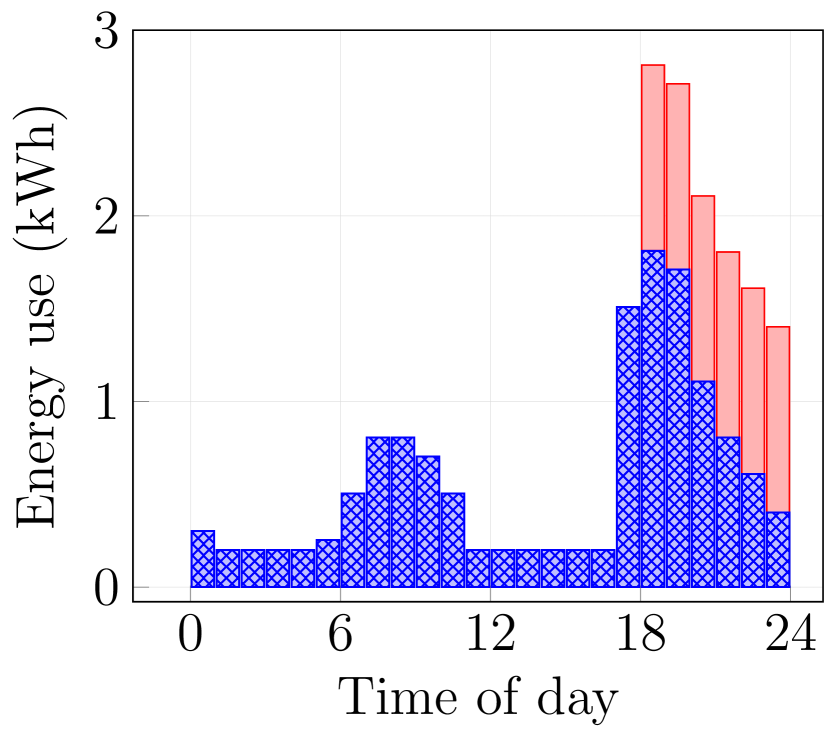
(a) Naïve pricing

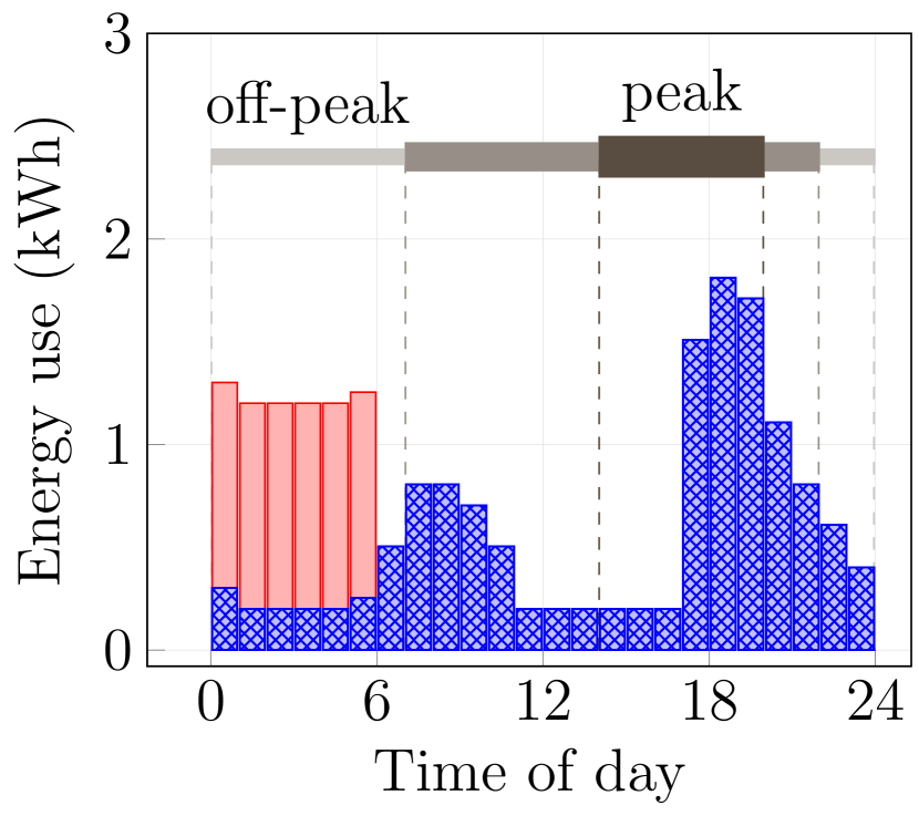
(b) Peak load pricing

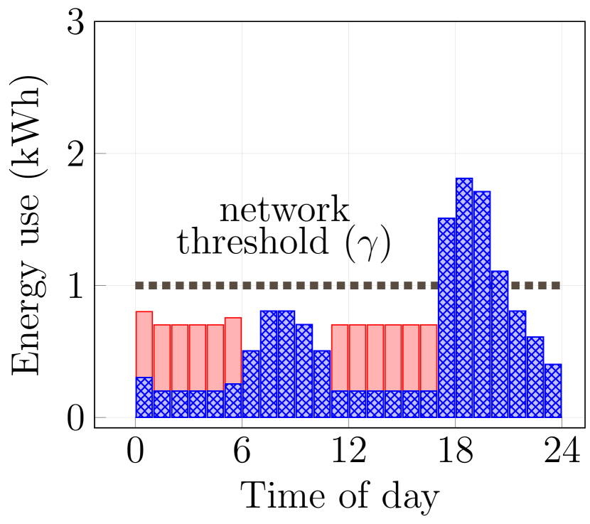
(c) Our pricing scheme

Figure 1: Demand over time of an average user. Blue and red bars represent demand due to must-run and controllable loads, respectively.

3 System & Security Model

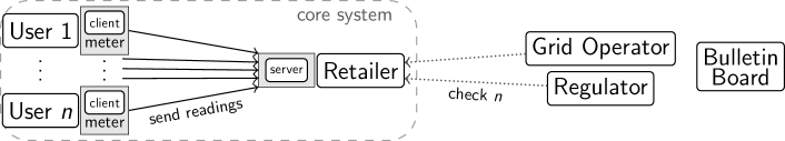
Figure 2: Entities in our system.

System model. Figure 2 depicts the different entities in our system. There is one power retailer and $n$ customers (or users). The retailer purchases electricity from power generators on the wholesale electricity market, and pays a fee to one or more grid operators for the use of their transmission and distribution networks. We assume that the regulator and grid operators know $n$, but that they are unable to observe the individual or total consumption of the retailer’s users. The retailer runs a server, and each user owns a smart meter, which runs a software application called a client that communicates with the server.

At the end of each period $t\in[k]$, each smart meter $i\in[n]$ sends the raw reading $y_{i\,t}$ to the retailer via a secure and highly available channel. At the end of the operational cycle, the retailer uses the same channel to send to each user a statement containing the total bill $B_{i}\in\mathbb{N}$, and for each period $t\in[k]$ both $y_{i\,t}$ and the sum $x^{*}_{t}$. The customer can then verify that $B_{i}=\sum_{t=1}^{k}p_{i\,t}(y_{i\,t},x^{*}_{t})x_{i\,t}$. However, the customer cannot verify $x^{*}_{t}$, which may allow the retailer to charge the peak rate incorrectly.

Threat model. The retailer is adversarial and interested in convincing users of accepting an incorrect bill $\tilde{B}_{i}$ such that $\tilde{B}_{i}>B_{i}$. We assume that the meters are secure, i.e., they produce readings that match the user’s true power consumption – otherwise, honest users would be able to report this to the regulator. The retailer can collude with a number of adversarial users who may generate arbitrary readings. Users can be adversarial because they have been bribed by the retailer, or they can be Sybil users created by the retailer. We assume that the regulator would notice if the retailer would create too many Sybils, so this number is limited in our model. Non-adversarial users are honest-but-curious, i.e., they will faithfully follow the protocol as described, but will attempt to use the information shared with them to learn the readings of other users. Finally, there is a public bulletin board which provides immutable and tamper-evident storage, e.g., a public blockchain.

Given this threat model, our first goal is allow users to detect incorrect bills. In particular, let $B^{*}_{i}$ be the bill for user $i$ if each adversarial user $j$ reports $x_{j\,t}=\delta_{t}$ in each period $t\in[k]$. An incorrect bill $\tilde{B}_{i}$ then satisfies $\tilde{B}_{i}>B^{*}_{i}$. In other words, the adversarial users should not be able to influence individual bills beyond reporting the maximum. Another goal is to hide private readings $x_{i\,t}$ from other honest-but-curious users. The final goal is efficiency, that is, the protocol can support a large number of users with practical performance.

3.1 Security Model

We let $\kappa$ be the security parameter by $\kappa$, and $\emptyset$ be the empty string. When $X$ is a set, $x\stackrel{{\scriptstyle{\scriptscriptstyle\$}}}{{\leftarrow}}X$ denotes the action of sampling an element uniformly at random from $X$. Let $\|$ denote an operation that concatenates two strings.

We define a privacy-preserving, transparent pricing (PPTP) scheme as one that consists of the four algorithms below.

• $(\text{P}_{\text{tp}},k_{r})\leftarrow\mathsf{Initialize}(1^{\kappa})$: run by the retailer. It takes as input the security parameter $\kappa$, and outputs the system parameters $\text{P}_{\text{tp}}$ and a secret key $k_{r}\in\mathcal{SK}_{\text{tp}}$ where $\mathcal{SK}_{\text{tp}}$ is the secret key space.

• $(r_{i\,t})_{i\in[n]}\leftarrow\mathsf{SlotSecretGen}(\text{P}_{\text{tp}},k_{r},t)$: run by the retailer. It takes as input the system parameters $\text{P}_{\text{tp}}$, the secret key $k_{r}$, and the time slot $t$, and outputs slot secrets $(r_{i\,t})_{i\in[n]}\in\mathcal{SS}_{\text{tp}}$ for $n$ users, where $\mathcal{SS}_{\text{tp}}$ is the slot secret space.

• $\text{E}_{t}\leftarrow\mathsf{EvidenceGen}(\text{P}_{\text{tp}},k_{r},(x_{i\,t})_{i\in[n]},t)$: run by the retailer. It takes as input the system parameters $\text{P}_{\text{tp}}$, secret key $k_{r}$, and the measurements $(x_{i\,t})_{i\in[n]}\in\mathcal{V}_{\text{tp}}$ of each user $i$ for time $t$, and outputs an evidence $\text{E}_{t}\in\mathcal{E}_{\text{tp}}$. Here, $\mathcal{E}_{\text{tp}}$ is the evidence space and $\mathcal{V}_{\text{tp}}$ is the measurement space.

• $\{0,1\}\leftarrow\mathsf{EvidenceVrf}(\text{P}_{\text{tp}},r_{i\,t},x_{i\,t},\text{E}_{t},t)$: run by each user. It takes as input the system parameters $\text{P}_{\text{tp}}$, slot secret $r_{i\,t}$, measurement $x_{i\,t}$ of user $i$ for time $t$, and the evidence $\text{E}_{t}$, and outputs True or False.

Given $(\text{P}_{\text{tp}},k_{r}):=\mathsf{Initialize}(1^{\kappa})$, $(r_{i\,t})_{i\in[n]}:=\mathsf{SlotSecretGen}(\text{P}_{\text{tp}},k_{r})$, a set of valid measurements $(x_{i\,t})_{i\in[n]}\in\mathcal{V}_{\text{tp}}$ for time slot $t$, the scheme is correct if $\mathsf{EvidenceVrf}((\text{P}_{\text{tp}},r_{j\,t},x_{j\,t},\mathsf{EvidenceGen}(\text{P}_{\text{tp}},k_{r},(x_{i\,t})_{i\in[n]},t),t)=1$, for any slot secret $r_{j\,t}\in(r_{i\,t})_{i\in[n]}$ and the corresponding measurement $x_{j\,t}\in(x_{i\,t})_{i\in[n]}$.

3.2 Security Properties

We define two properties of PPTP: transparency and privacy. For simplicity, we focus on a single operational cycle.

Transparency. This property means that each honest user $i\in[n]$ is able to verify that a bill $\tilde{B}_{i}$ is incorrect if $\tilde{B}_{i}>B^{*}_{i}$, where $B^{*}_{i}$ is the worst-case bill defined earlier in the section. Furthermore, the user can check if $\tilde{B}_{i}$ contains an incorrect measurement $\bar{x}_{i\,t}$, i.e., $\bar{x}_{i\,t}>x_{i\,t}$ or $\bar{x}_{i\,t}>\delta_{t}$. Finally, a dishonest user cannot blame the retailer for misbehavior if it has behaved honestly.

We formulate transparency through a two-stage game $\mathsf{Game}^{\mathsf{Trans}}_{\mathsf{PPTP},\mathcal{A}}$ running between a challenger and an adversary $\mathcal{A}$. In the first stage, the adversary can run the PPTP scheme herself with the secret key $k_{r}$ and measurements of her own choice, and outputs a time slot $t^{*}$ as challenge request. The challenger then randomly samples a set of honest measurements $\vec{x}_{t^{*}}=(x_{i\,t^{*}})_{i\in[n]}\stackrel{{\scriptstyle{\scriptscriptstyle\$}}}{{\leftarrow}}\mathcal{V}_{\text{tp}}$ which are sent to $\mathcal{A}$. The goal of $\mathcal{A}$ is to generate a valid evidence $\bar{\text{E}}_{t^{*}}$ for a set of measurements $\bar{\vec{x}}_{t^{*}}=(\bar{x}_{i\,t^{*}})_{i\in[n]}$, such that $\bar{\vec{x}}_{t^{*}}\neq\vec{x}_{t^{*}}$, which can pass the verification for an honest user $j^{*}$’s measurement $x_{j^{*},t^{*}}\in\vec{x}_{t^{*}}$, meaning that $\mathsf{EvidenceVrf}(\text{P}_{\text{tp}},r_{j\,t^{*}},x_{j\,t^{*}},\bar{\text{E}}_{t^{*}},t^{*})=1$.

Privacy. This property means that a user $i$ cannot learn privacy-sensitive meter readings $x_{j\,t}$ of another user $j\in[n]\backslash\{i\}$ for any $t\in[k]$.

We define a game $\mathsf{Game}^{\mathsf{Priv}}_{\mathsf{PPTP},\mathcal{A}}$ to formulate the privacy via indistinguishability. The adversary $\mathcal{A}$ chooses measurements $(x_{i\,t})_{i\in[n],t\in[k]}$ for all users, and an honest user $j^{*}$ and time slot $t^{*}$ as the challenge in the game. The challenger selects two values $x^{0}_{j^{*}\,t^{*}},x^{0}_{j^{*}\,t^{*}}$ that lead to the same bills for all users $i\neq j^{*}$. Specifically, it sets $x^{0}_{j^{*}\,t^{*}}:=x_{j^{*}\,t^{*}}$, and $x^{1}_{j^{*},t^{*}}\stackrel{{\scriptstyle{\scriptscriptstyle\$}}}{{\leftarrow}}\mathcal{V}_{\text{tp}}$, such that $x^{0}_{j^{*},t^{*}}\neq x^{1}_{j^{*},t^{*}}$ and $(\bigwedge^{n}_{i=1,i\neq j^{*}}B^{0}_{i}=B^{1}_{i})=1$, where $B^{b}_{i}=p_{i\,t^{*}}(x_{i\,t^{*}},x^{b,*}_{t^{*}})x_{i\,t^{*}}+\sum_{t=1,t\neq t^{*}}^{k}p_{i\,t}(x_{i\,t},x^{*}_{t})x_{i\,t}$ and $x^{b,*}_{t^{*}}=\min(x^{b}_{j^{*},t^{*}},d_{t^{*}})+\sum_{i=1,i\neq j^{*}}^{n}\min(x_{i\,t^{*}},d_{t^{*}})$. Next, the challenger generates the evidence for time $t^{*}$ based on $(x_{i\,t^{*}})_{i\in[n],i\neq j^{*}}||x^{b}_{j^{*}\,t^{*}}$ and $b\stackrel{{\scriptstyle{\scriptscriptstyle\$}}}{{\leftarrow}}\{0,1\}$. The goal of $\mathcal{A}$ in this game is to distinguish whether her measurement $x_{j^{*}\,t^{*}}$ is used to generate the challenge evidence $\text{E}_{t^{*}}$. Note that the constraint that the values chosen by the challenger leads to the same bill for users $i\neq j^{*}$ is important. Otherwise, the distinct bills would allow the adversary to trivially distinguish the bit $b$. During the game, the adversary can ask oracle $\mathcal{O}_{\mathsf{EG}}$ to get the evidences for any measurements, and oracle $\mathcal{O}_{\mathsf{C}}$ to reveal the slot secrets. But it cannot ask either $\mathcal{O}_{\mathsf{EG}}(\cdot,t^{*})$ or $\mathcal{O}_{\mathsf{C}}(j^{*},t^{*})$.

$\underline{\mathsf{Game}^{\mathsf{Trans}}_{\mathsf{PPTP},\mathcal{A}}(\kappa)}$	$\underline{\mathsf{Game}^{\mathsf{Priv}}_{\mathsf{PPTP},\mathcal{A}}(\kappa})$
$\mathsf{QL}:=\emptyset$	$\mathsf{QL}:=\emptyset$; $\mathsf{CL}:=\emptyset$; $b\stackrel{{\scriptstyle{\scriptscriptstyle\$}}}{{\leftarrow}}\{0,1\}$
$(\text{P}_{\text{tp}},k_{r})\leftarrow\mathsf{Initialize}(1^{\kappa})$	$(\text{P}_{\text{tp}},k_{r})\leftarrow\mathsf{Initialize}(1^{\kappa})$
$(state,t^{*})\leftarrow\mathcal{A}(\text{P}_{\text{tp}},k_{r})$	$(state,j^{*},t^{*},(x_{i\,t})_{i\in[n],t\in[k]})\leftarrow\mathcal{A}^{\mathcal{O}_{\mathsf{EG}}(\cdot,\cdot),\mathcal{O}_{\mathsf{C}}(\cdot,\cdot)}(\text{P}_{\text{tp}})$
$\vec{x}_{t^{*}}=(x_{i\,t^{*}})_{i\in[n]}\stackrel{{\scriptstyle{\scriptscriptstyle\$}}}{{\leftarrow}}\mathcal{V}_{\text{tp}}$, s.t., $x_{i\,t^{*}}\leq\delta_{t}$ for $i\in[n]$	$x^{0}_{j^{*}\,t^{*}}:=x_{j^{*}\,t^{*}}$
$(\bar{\text{E}}_{t^{*}},(\bar{x}_{i\,t^{*}})_{i\in[n]},j^{*})\leftarrow\mathcal{A}(\text{P}_{\text{tp}},k_{r},state,(x_{i\,t^{*}})_{i\in[n]})$	$x^{1}_{j^{*}\,t^{*}}\stackrel{{\scriptstyle{\scriptscriptstyle\$}}}{{\leftarrow}}\mathcal{V}_{\text{tp}}$, s.t., $(x^{0}_{j^{*}\,t^{*}}\neq x^{1}_{j^{*}\,t^{*}})$ and $(\bigwedge^{n}_{i=1,i\neq j^{*}}B^{0}_{i}=B^{1}_{i})=1$
$\bar{\vec{x}}_{t^{*}}=(\bar{x}_{i\,t^{*}})_{i\in[n]}$	$\quad\text{where }B^{b}_{i}=p_{i\,t^{*}}(x_{i\,t^{*}},x^{b,*}_{t^{*}})x_{i\,t^{*}}+\sum_{t=1,t\neq t^{*}}^{k}p_{i\,t}(x_{i\,t},x^{*}_{t})x_{i\,t}$
Return $(\vec{x}_{t^{*}}\neq\bar{\vec{x}}_{t^{*}})\wedge(\bigvee^{n}_{i=1}\bar{x}_{i\,t^{*}}>\delta_{t})$	$\quad\text{and }x^{b,*}_{t^{*}}=\min(x^{b}_{j^{*},t^{*}},\delta_{t^{*}})+\sum_{i=1,i\neq j^{*}}^{n}\min(x_{i\,t^{*}},\delta_{t^{*}})$
$\quad\wedge(\bar{\text{E}}_{t^{*}}=\mathsf{EvidenceGen}(\text{P}_{\text{tp}},k_{r},(\bar{x}_{i\,t^{*}})_{i\in[n]},t^{*})$	$\text{E}_{t^{*}}:=\mathsf{EvidenceGen}(\text{P}_{\text{tp}},k_{r},((x_{i\,t^{*}})_{i\in[n]\backslash j^{*}}||x^{b}_{j^{*},t^{*}}),t^{*})$
$\quad\wedge(\mathsf{EvidenceVrf}(\text{P}_{\text{tp}},r_{j^{*}\,t^{*}},x_{j^{*}\,t^{*}},\bar{\text{E}}_{t^{*}},t^{*})=1)$	$b^{\prime}\leftarrow\mathcal{A}^{\mathcal{O}_{\mathsf{EG}}(\cdot,\cdot),\mathcal{O}_{\mathsf{C}}(\cdot,\cdot)}(\text{P}_{\text{tp}},\text{E}_{t^{*}},state)$
	Return $(b=b^{\prime})\wedge(t^{*}\notin\mathsf{QL})\wedge(r_{j^{*},t^{*}}\notin\mathsf{CL})$
$\underline{\mathcal{O}_{\mathsf{EG}}((x_{i\,t})_{i\in[n]},t)}$	$\underline{\mathcal{O}_{\mathsf{C}}(i,t)}$
$E_{t}:=\mathsf{EvidenceGen}(\text{P}_{\text{tp}},k_{r},(x_{i\,t})_{i\in[n]},t)$	$(r_{i\,t})_{i\in[n]}:=\mathsf{SlotSecretGen}(\text{P}_{\text{tp}},k_{r},t)$
$(E_{t},t,(x_{i\,t})_{i\in[n]})\rightarrow\mathsf{QL}$	$r_{i\,t}\rightarrow\mathsf{CL}$
Return $\text{E}_{t}$	Return $r_{i\,t}$

Definition 1

A privacy-preserving transparent pricing scheme $\mathsf{PPTP}$ is secure if the advantages $\mathsf{Adv}^{\mathsf{Trans}}_{\mathsf{PPTP},\mathcal{A}}(\kappa)=\Pr[\mathsf{Game}^{\mathsf{Trans}}_{\mathsf{PPTP},\mathcal{A}}=1]$ and $\mathsf{Adv}^{\mathsf{Priv}}_{\mathsf{PPTP},\mathcal{A}}(\kappa)=\left|\Pr[\mathsf{Game}^{\mathsf{Priv}}_{\mathsf{PPTP},\mathcal{A}}(\kappa)=1]-1/2\right|$ of any PPT adversaries $\mathcal{A}$ in the corresponding games are negligible.

4 Baseline Protocol

In this section, we present a simple instantiation of PPTP. This baseline protocol meets the security definition above. In particular, the retailer creates a commitment and zero-knowledge range proof for each user’s measurement, and shares the full set of commitments and proofs with all users. Each honest user verifies all the steps of the protocol to detect misbehavior. This protocol incurs a large performance overhead, which we address in next section with a more efficient protocol. In the following, we focus on the algorithms for a single time period $t\in[k]$, and discuss how to generalize it to a full operation cycle.

4.1 Preliminaries

We briefly review the syntax and security properties of the cryptographic primitives used in our protocol.

Commitment Scheme. A commitment scheme $\mathsf{COM}$ consists of two algorithms. $\mathsf{COM.Setup}(1^{\kappa})$ takes as input the security parameter $1^{\kappa}$, and outputs commitment parameters $\text{P}_{\text{c}}$. The algorithm $\mathsf{COM.Commit}(\text{P}_{\text{c}},v,r)$ takes as input parameters $\text{P}_{\text{c}}$, a value $v$, and randomness $r$, and outputs a commitment $c$. The scheme is hiding when $c$ reveals nothing of the committed value, and binding when the commitment cannot be opened with two different random values. The scheme is collision-resistant if for any $(v_{0},v_{1})\in\mathcal{V}_{\text{c}}$ and $(r_{0},r_{1})\in\mathcal{R}_{\text{c}}$ such that $v_{0}\neq v_{1}$, the probability that $\mathsf{COM.Commit}(\text{P}_{\text{c}},v_{0},r_{0})=\mathsf{COM.Commit}(\text{P}_{\text{c}},v_{1},r_{1})$ is negligible. Finally, the scheme is (additively) homomorphic if, for any $(v_{0},v_{1})\in\mathcal{V}_{\text{c}}$ and $(r_{0},r_{1})\in\mathcal{R}_{\text{c}}$, we have

$$\mathsf{COM.Commit}(\text{P}_{\text{c}},v_{0},r_{0})+\mathsf{COM.Commit}(\text{P}_{\text{c}},v_{1},r_{1})=\mathsf{COM.Commit}(\text{P}_{\text{c}},v_{0}+v_{1},r_{0}+r_{1}).$$

Non-interactive Zero-knowledge. Let $\mathsf{R_{zk}}$ be an efficiently computable relation of the form $(st,w)\in\mathsf{R_{zk}}$, where $st$ is the statement and $w$ is the witness of $st$. A non-interactive proof system $\mathsf{NIZK}$ for $\mathsf{R_{zk}}$ consists of three algorithms. $\mathsf{NIZK.Setup}(1^{\kappa})$ which takes as input the security parameter $1^{\kappa}$ and outputs the system parameters $\text{P}_{\text{zk}}$. $\mathsf{NIZK.Prv}(\text{P}_{\text{zk}},st,w)$ takes as input system parameters $\text{P}_{\text{zk}}$ and a pair $(st,w)$ and outputs a proof $\pi$. $\mathsf{NIZK.Vrf}(\text{P}_{\text{zk}},st,\pi)$ takes as input $\text{P}_{\text{zk}}$, a statement $st$, and a proof $\pi$, and outputs True $(1)$ or False $(0)$.

The proof system $\mathsf{NIZK}$ satisfies zero-knowledge if the generated proofs reveal nothing regarding the corresponding witnesses, and simulation-extractability if for any proof generated by the adversary, there exists an efficient algorithm to extract the corresponding witnesses with a trap door. In this work, we use $\mathsf{NIZK}$ over the family of relations $\mathsf{R_{zk}}=(\mathcal{RL}_{\mathsf{v}_{\text{max}}})_{\mathsf{v}_{\text{max}}\in\mathbb{N}}$, where $\mathsf{v}_{\text{max}}$ can be either $\gamma_{t}$ or $\delta_{t}$, and

$$\mathcal{RL}_{\mathsf{v}_{\text{max}}}=\{(c,\mathsf{v}_{\text{max}}),(v,r)\big{|}c=\mathsf{COM.Commit}(\text{P}_{\text{c}},v,r)\wedge v\in[0,\mathsf{v}_{\text{max}}]\}.$$

Pseudo-Random Functions. A pseudo-random function (PRF) family consists of two algorithms. $\mathsf{PRF.KGen}(1^{\kappa})$ is takes as input the security parameter $1^{\kappa}$ and outputs a random key $k$. $\mathsf{PRF.Eval}(k,x)$ is takes as input the random key $k$ and a message $x$, and outputs a pseudo-random value $r$.

4.2 Instantiation

The four main algorithms of Section 3 are instantiated as follows.

• $(\text{P}_{\text{tp}},k_{r})\leftarrow\mathsf{Initialize}(1^{\kappa})$: this algorithm generates the secret key $k_{r}:=\mathsf{PRF.KGen}(1^{\kappa})$, and initializes the commitment and non-interactive zero-knowledge schemes as $\text{P}_{\text{c}}:=\mathsf{COM.Setup}(1^{\kappa})$ and $\text{P}_{\text{zk}}:=\mathsf{NIZK.Setup}(1^{\kappa})$, respectively. The retailer publishes the system parameters $\text{P}_{\text{tp}}=(\text{P}_{\text{c}},\text{P}_{\text{zk}},\alpha_{t},\beta_{t},\gamma_{t},\delta_{t})$ and keeps the secret key $k_{r}$ private.

• $(r_{i\,t})_{i\in[n]}\leftarrow\mathsf{SlotSecretGen}(\text{P}_{\text{tp}},k_{r},t)$: this algorithm uses the retailer’s secret key to generate the slot secrets as $r_{i\,t}:=\mathsf{PRF.Eval}(k_{r},i||t)$ for $i\in[n]$. Each slot secret $r_{i\,t}$ is sent to the corresponding user $i$ via a secure channel and is stored privately by the retailer and user $i$.

• $\text{E}_{t}\leftarrow\mathsf{EvidenceGen}(\text{P}_{\text{tp}},(x_{i\,t},r_{i\,t})_{i\in[n]},t)$: this algorithm computes for each user $c_{i\,t}:=\mathsf{COM.Commit}(\text{P}_{\text{c}},x_{i\,t},r_{i\,t})$ and generates the proof $\pi_{i\,t}:=\mathsf{NIZK.Prv}(\text{P}_{\text{zk}},st,w)$ for the statement $st=(c_{i\,t},\delta_{t})$ and witness $w=(x_{i\,t},r_{i\,t})$. The retailer computes the sum of the values $x_{t}^{*}=\sum_{i=1}^{n}x_{i\,t}$, the sum of the random seeds $r_{t}^{*}=\sum_{i=1}^{n}r_{i\,t}$, $c_{t}^{*}:=\mathsf{COM.Commit}(\text{P}_{\text{c}},x_{t}^{*},r_{t}^{*})$, and a proof $\pi_{t}^{*}:=\mathsf{NIZK.Prv}(\text{P}_{\text{zk}},st,w)$ for $st=(c_{t}^{*},\gamma_{t})$ and witness $w=(x_{t}^{*},r_{t}^{*})$. Finally, the retailer shares $\text{E}_{t}=(c_{t}^{*},\pi_{t}^{*},(c_{i\,t},\pi_{i\,t})_{i\in[n]})$ with each user, and puts a hash $h_{t}=H(E_{t})$ on the bulletin board.

• $\{0,1\}\leftarrow\mathsf{EvidenceVrf}(\text{P}_{\text{tp}},r_{i\,t},x_{i\,t},\text{E}_{t},t)$: this algorithm executes four subroutines, each taking parts of $\text{E}_{t}=(c_{t}^{*},\pi_{t}^{*},(c_{i\,t},\pi_{i\,t})_{i\in[n]})$ as input, and returns True if all four subroutines return 1.

  • $\{0,1\}\leftarrow\mathsf{VerifyConsistency(}\text{E}_{t},h\texttt{)}$: computes $\bar{h}=H(\text{E}_{t})$, and outputs True if $\bar{h}=h$, and False otherwise.

  • $\{0,1\}\leftarrow\mathsf{VerifyCommitment(}\text{P}_{\text{c}},x_{i\,t},c_{i\,t},t\texttt{)}$: computes $\bar{c}_{i\,t}:=\mathsf{COM.Commit}(\text{P}_{\text{c}},x_{i\,t},r_{i\,t})$ and outputs True if $\bar{c}_{i\,t}=c_{i\,t}$, and False otherwise.

  • $\{0,1\}\leftarrow\mathsf{VerifySum(}\text{P}_{\text{zk}},c_{t}^{*},\pi_{t}^{*},(c_{i\,t})_{i\in[n]}\texttt{)}$: computes $\bar{c}_{t}^{*}=\sum_{i=1}^{n}c_{i\,t}$. It checks if $\bar{c}^{*}=c^{*}$. It then checks that $c^{*}$ and $\pi_{t}^{*}$ match, and executes $\mathsf{NIZK.Vrf}(\text{P}_{\text{zk}},st,\pi_{t}^{*})$ for the statement $st=(c^{*},\gamma_{t})$. The functions outputs True if all three checks are successful, and False otherwise.

  • $\{0,1\}\leftarrow\mathsf{VerifyRangeProofs(}\text{P}_{\text{zk}},(c_{i\,t},\pi_{i\,t})_{i\in[n]}\texttt{)}$: checks that for each $i$, the commitment $c_{i\,t}$ and the proof $\pi_{t}$ match, then executes $\mathsf{NIZK.Vrf}(\text{P}_{\text{zk}},st,\pi_{i\,t})$ for the statement $st=(c_{i\,t},\delta_{t})$. It outputs True if all proofs are valid and match the commitment, and False otherwise.

Operational cycles. For a full operational cycle, the protocol above is executed for every time period $t\in[k]$. The retailer computes $B_{i}$ and sends it to each user $i\in[n]$, who then verifies the bill since she knows $x_{i\,t}$ and $x^{*}_{t}$ for each time period.

4.3 Security Analysis

The baseline protocol described in this section is secure according to Definition 1. The proofs for the following two theorems are included in the Appendix Appendix B: Security Proofs.

Theorem 4.1

If the commitment scheme $\mathsf{COM}$ is additively homomorphic and satisfies binding property, and non-interactive zero-knowledge proof system $\mathsf{NIZK}$ is simulation-extractable, then the baseline protocol provides transparency.

Theorem 4.2

If the commitment scheme $\mathsf{COM}$ is additively homomorphic and satisfies hiding property, the non-interactive zero-knowledge proof system $\mathsf{NIZK}$ provides zero-knowledge, and pseudo-random function family $\mathsf{PRF}$ is secure, then the baseline protocol satisfies privacy.

4.4 Performance Analysis

We analyze the computation cost of the protocol in terms of the number of invocations to the cryptographic functions, and the bandwidth cost in terms of the sizes of the messages sent over the network. We ignore the initiation cost and the cost of users sending measurements to the retailer, as these are independent of the implementation. In the following, $M_{c}$, $M_{\pi}$, $M_{h}$ respectively denote the message size of the commitments, proofs, and hashes.

The total costs per time slot for each entity are summarized in Table 2. The server has to execute the $\mathsf{COM.Commit}$ and $\mathsf{NIZK.Prv}$ $n+1$ times in the $\mathsf{EvidenceGen}$ algorithm: $n$ times for each client’s measurement $x_{i\,t}$ and once for the sum $x^{*}_{t}$. The $n+1$ commitments and proofs are sent to each of the $n$ clients, meaning that a message of size $(n+1)(M_{c}+M_{\pi})$ is sent $n$ times. The server also computes $H(\text{E}_{t})$, and sends this hash to the bulletin board. Each client receives a single message of size $n(M_{c}+M_{\pi})$, and downloads the hash from the bulletin board for verification. The client then 1) verifies the commitment of its own measurement by executing $\mathsf{COM.Commit}$ and checking whether its output matches the value sent by the retailer, 2) executes $\mathsf{NIZK.Vrf}$ on each of the proofs, and 3) check whether the hash of the result matches the one on the bulletin board. The load on the bulletin board consists of receiving a single hash from the retailer, and sending it to the $n$ users.

Table 2: Performance cost of the baseline solution.

Entity Computation Bandwidth $\mathsf{COM.Commit}$ $\mathsf{NIZK.Prv}$ $\mathsf{NIZK.Vrf}$ Server $n+1$ $n+1$ $0$ $n(n+1)(M_{c}+M_{\pi})+M_{h}$ Client $1$ $0$ $n+1$ $(n+1)(M_{c}+M_{\pi})+M_{h}$ Bulletin Board $0$ $0$ $0$ $(n+1)M_{h}$

4.5 Discussion

We consider the computation cost at the server, which increases linearly in $n$, to be acceptable because the server is often equipped with powerful CPUs, and the operations are parallelizable. The bandwidth cost increases quadratically, but the server can offload the messages to a cloud storage or content delivery network that can distribute the messages in a scalable and cost-effective fashion. We discuss a blockchain-based extension to the baseline protocol that reduces the costs at the client, which is important since the clients are likely running on edge devices close to the meters, or even running directly on the meter firmware.

Table 3: Performance cost of the blockchain solution. $\mathsf{BC}$ represents the processing of read requests at the blockchain smart contract. $M_{bc}$ is the message containing the blockhain proof that a commitment is stored in the chain.

Entity Computation Bandwidth $\mathsf{COM.Commit}$ $\mathsf{NIZK.Prv}$ $\mathsf{NIZK.Vrf}$ $\mathsf{BC}$ Server $n+1$ $n+1$ $0$ $0$ $(n+1)(M_{c}+M_{\pi})$ Client $1$ $0$ $0$ $1$ $M_{c}+M_{bc}$ Bulletin Board $0$ $0$ $n+1$ $n+1$ $(2n+1)M_{c}+nM_{bc}+(n+1)M_{\pi}$

We note that for verification, only the $\mathsf{VerifyCommitment}$ algorithm requires the private input. In other words, most of the verification can be done publicly by another party without compromising client privacy. The $\mathsf{VerifyRangeProof}$ algorithm, which is the most expensive, can therefore be performed by a trusted third party with more resources than the client. As a first improvement over the baseline solution, we propose to leverage a blockchain as the trusted party, and implement the range proof verification in a smart contract.

The server sends the proofs and commitments to a blockchain smart contract, which executes $\mathsf{VerifyConsistency}$, $\mathsf{VerifySum}$, and $\mathsf{VerifyRangeProofs}$. If the verifications pass, the blockchain stores the messages. The client $i$ only computes the commitment $c_{i\,t}$ using its own measurement $x_{i\,t}$, and verifies that it was included in the blockchain by reading blockchain storage directly without incurring consensus overhead. The client does not need to run $\mathsf{NIZK.Vrf}$ on any of the other users’ range proofs, but the trade-off here is that the blockchain incurs significant overhead: generating $n$ proofs for read requests from the user, and executing the smart contract for verification. We summarize the cost for each entity in Table 3 in the Appendix.

5 Merkle Tree Protocol

As discussed in Section 4.5, the baseline solution of Section 4 can be improved by offloading all range proof verification to a trusted third party such as the bulletin board. However, this puts a large computational burden on the bulletin board – far beyond the capacity of, for example, the Ethereum blockchain. In this section, we take inspiration from Certificate Transparency [5] and describe another PPTP instantiation based on a modified Merkle tree. The protocol reduces the communication and computation costs at the user, and therefore is more practical. In each period the retailer sends to each user a proof of the inclusion and a range proof for the sum $x^{*}_{t}$, which due to the homomorphism of our commitment scheme corresponds to the value in the root of the tree.

5.1 Overview

Merkle trees are an extension of binary trees. For any node $v$, let $\textsc{left}(v)$ be its first child and $\textsc{right}(v)$ its second child. If node $v$ has no second child, then $\textsc{right}(v)=0$, and if it also has no first child then $\textsc{left}(v)=0$. In the original Merkle tree, each node $v$ contains a hash value $h_{v}$ of its children. We modify it by storing at each node $v$ a commitment $c_{v}$. For each user $i\in[n]$ we set the commitment in the $i$th leaf equal to $c_{i}=\mathsf{COM.Commit}(\text{P}_{\text{c}},x_{i\,t},r_{i\,t})$. The commitments in the other nodes are computed as:

$$\begin{array}[]{c}c_{v}=c_{\textsc{left}(v)}+c_{\textsc{right}(v)},\end{array}$$ (3)

such that and $c_{0}=\mathsf{COM.Commit}(\text{P}_{\text{c}},0,0)$. The inclusion proof for node $i$ includes the root, $i$’s leaf, the intermediate nodes that lie on the path between them, and the children of these nodes. Figure 3 shows an example, where the green nodes represent the path between the leaf and the root and the yellow nodes the children of those nodes.

Assumptions. In this section, we describe a protocol that is secure under the following assumptions. There are a number of powerful entities, called auditors, that perform verification on behalf of the users. In the following, we assume that auditors do not share measurements themselves (although in practice a single entity may act as a user and an auditor). At least one auditor is honest, and at most $f$ are dishonest. Furthermore, the maximum time for an auditor to finish its verification and have its messages stored on the bulletin board, $T$, is known. We discuss other protocols that do not rely on auditors in the Appendix Appendix A: A Protocol Without Auditors.

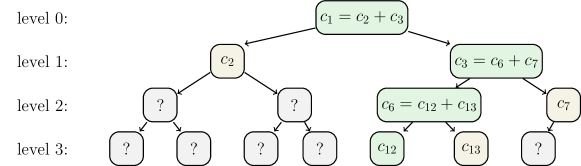
Figure 3: Example of a modified Merkle tree with 7 leaves.

5.2 Instantiation

The four algorithms of Section 3 are instantiated as follows.

• $\mathsf{Initialize},\ \mathsf{SlotSecretGen}$: they are the same as in Section 4.

• $\text{E}_{t}\leftarrow\mathsf{EvidenceGen}(\text{P}_{\text{tp}},(x_{i\,t},r_{i\,t})_{i\in[n]},t)$: this algorithm constructs a Merkle tree described above, using the measurements and slot randomness as input. For each user, the evidence $E_{t}$ contains the inclusion proof $G$ and a zero-knowledge proof $\pi_{t}^{*}$ that the sum $x_{t}^{*}$ (whose commitment $c_{t}^{*}$ is the root of $G$) is within the range $[0,\gamma_{t}]$. For auditors, the evidence also includes the commitments and range proofs $(c_{i\,t},\pi_{i\,t})$ for all leaf nodes $i\in[n]$. The retailer also uploads the commitment in the root node to the public bulletin board as $c_{h}$.

• $\{0,1\}\leftarrow\mathsf{EvidenceVrf}(\text{P}_{\text{tp}},r_{i\,t},x_{i\,t},\text{E}_{t},t)$: this algorithm consists of two phases. In the first phase, it execute the following subroutines.

  • $\{0,1\}\leftarrow\mathsf{VerifyConsistency(}G,c_{h}\texttt{)}$: verifies that the value of $c_{h}$ on the bulletin board matches with the root of the inclusion proof $G$.

  • $\{0,1\}\leftarrow\mathsf{VerifyCommitment(}\text{P}_{\text{c}},r_{i\,t},x_{i\,t},G\texttt{)}$: if the user is an auditor, returns True. Else, it computes $\bar{c}_{i\,t}:=\mathsf{COM.Commit}(\text{P}_{\text{c}},x_{i\,t},r_{i\,t})$, and verifies that $\bar{c}_{i\,t}=c_{v}$, where $v$ is the leaf node in the user’s inclusion proof $G$.

  • $\{0,1\}\leftarrow\mathsf{VerifyInclusionProof(}G\texttt{)}$: if the user is an auditor, returns True. Else, it verifies that the inclusion proof is valid, i.e., that the commitment $c$ in each intermediate core node $v\in G$ indeed follows from applying (3) to the commitments in $v$’s children.

  • $\{0,1\}\leftarrow\mathsf{VerifySum(}\text{P}_{\text{zk}},G,\pi_{t}^{*}\texttt{)}$: if the user is an auditor, returns True. Else, it verifies that the proof $\pi_{t}^{*}$ matches the commitment $c_{t}^{*}$ in the root of $G$, and executes $\mathsf{NIZK.Vrf}(\text{P}_{\text{zk}},st,\pi_{t}^{*})$ for the statement $st=(c_{t}^{*},\gamma_{t})$.

  • $\{0,1\}\leftarrow\mathsf{VerifyTree}(\text{P}_{\text{zk}},(c_{i\,t},\pi_{i\,t})_{i\in[n]})$: if the user is not an auditor, returns True. Else, it executes $\mathsf{VerifyRangeProofs}(\text{P}_{\text{zk}},(c_{i\,t},\pi_{i\,t})_{i\in[n]})$ from Section 4 for each user $i\in[n]$. Then, it checks whether the non-leaf nodes of the tree are correct, i.e., whether they follow from applying (3). It returns True if all checks are successful, and False otherwise.

  In the second phase, if the user is an auditor, it signs and publishes a message to the bulletin board: a failed range proof for a leaf node if it exists, the value $1$ if all four subroutines in the fist phase succeed, or an empty message otherwise. The algorithm then returns true or false depending on the result of the first phase. The non-auditor user checks if there is a proof of incorrect range in the bulletin board, if yes, it verifies the proof and returns false. Otherwise, it waits until there are $f+1$ signed empty messages on the bulletin and returns True, or returns False after time $T$.

5.3 Security Analysis

We show that this protocol is a secure PPTP, by proving the following theorems. The proofs are included in the Appendix.

Theorem 5.1

If the commitment scheme $\mathsf{COM}$ is additively homomorphic and satisfies binding property, and non-interactive zero-knowledge proof system $\mathsf{NIZK}$ is simulation-extractable, and the assumptions about $f$ and $T$ hold, then the Merkle tree protocol provides transparency.

Theorem 5.2

With the same assumptions in Theorem 4.2, the Merkle tree protocol satisfies privacy.

5.4 Performance Analysis

We analyze the performance of the Merkle tree protocol using the same metrics as in the analysis of the baseline protocol. For simplicty, we assume $n=2^{m}$ for some $m\in\mathbb{N}$, so that the total number of nodes in the tree equals $2^{m+1}-1=2n-1$. The retailer generates commitments for all $2n-1$ nodes and generates range proofs for the root and the $n$ leaf nodes. It only sends the commitments for the nodes in the inclusion proof – this consists of $m=\log_{2}n$ nodes on the path and $m+1$ children, so $2m+1$ in total. Table 4 summarizes the cost.

We can also extend the protocol to use a blockchain as described in Section 4.5. In particular, we can offload the range proofs to the smart contracts, hence making the blockchain an auditor.

Table 4: Performance cost of the Merkle tree solution, assuming $m=\log_{2}(n)$ and $f+1$ auditors who each report to the bulletin board. Note that a user can simultaneously act as a normal client and as an auditor.

Entity Computation Bandwidth $\mathsf{COM.Commit}$ $\mathsf{NIZK.Prv}$ $\mathsf{NIZK.Vrf}$ Server $2n-1$ $n+1$ $0$ $(n+1)(f+1)(M_{c}+M_{\pi})+n(2m+1)M_{c}$ Normal Client $1$ $0$ $1$ $(2m+1)M_{c}+(f+1)M_{bc}$ Auditor $0$ $0$ $n$ $(n+1)(M_{c}+M_{\pi})+M_{bc}$ Bulletin Board $0$ $0$ $0$ $(n+1)(f+1)M_{bc}$

6 Implementation

We implement both the baseline and Merkle tree protocol in Go. To do so, we extend the zero-knowledge range proof library by Morais et al. [10]. In particular, we use their implementation of Bulletproofs [4] which uses Pedersen commitment with the secp256k1 elliptic curve [3] as a commitment scheme. We parallelize proof generations and verification by exploiting Go’s multi-threading. We release the source code for our experiments at https://github.com/aungmawjj/zkrp.

We evaluate the performance of our protocols in terms of the computation and bandwidth cost. We also examine how the performance scales with more hardware resources. There are no baselines from the related literature in our evaluation, because we are unaware of other protocols that address the same problem and have the same security guarantee as ours. We run the retailer’s server on AWS EC2 with varying numbers of cores. We run the client on a Raspberry Pi (RPI) 3 with 4 CPUs and 1GB RAM.

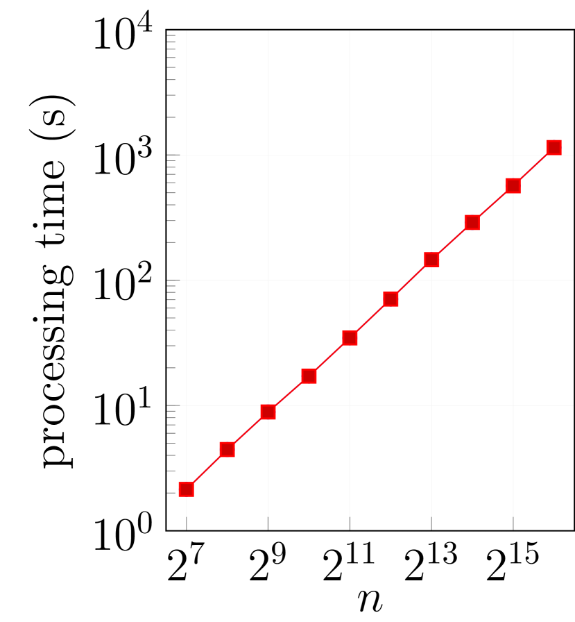
(a)

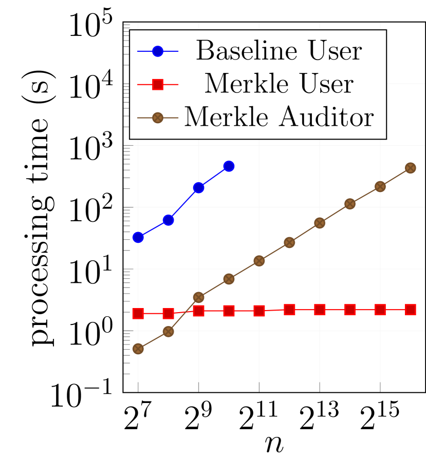
(b)

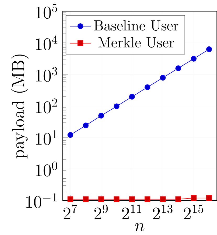
(c)

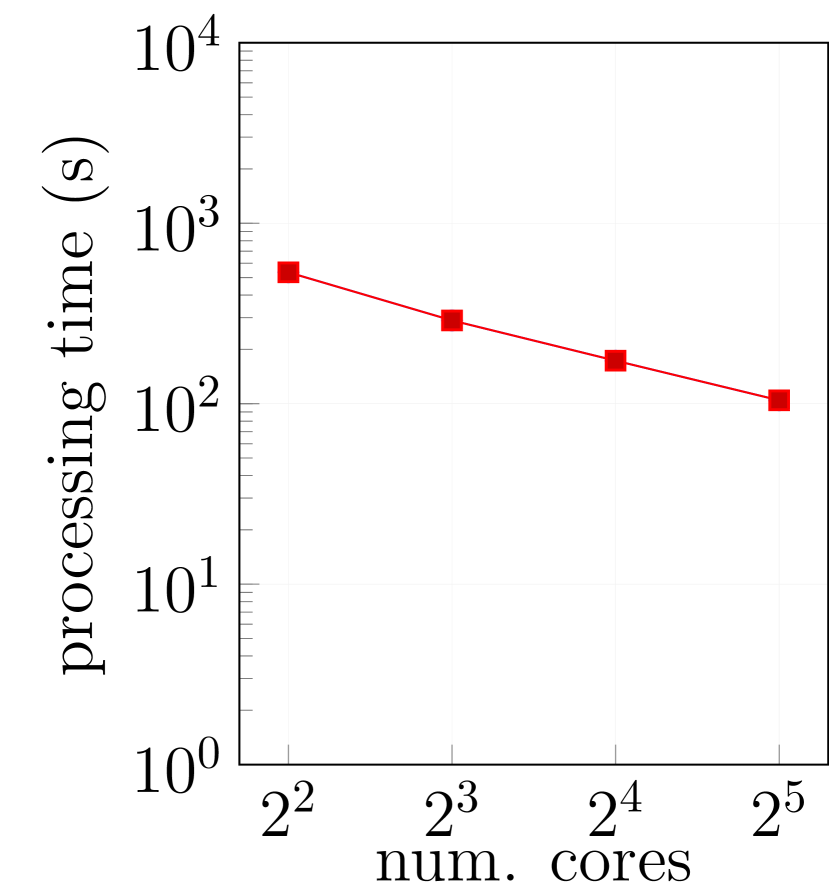
(d)

Figure 4: (a) Proof generation times, (b) proof verification times, (c) network cost. Experiments taking longer than $20$ minutes are not included. (d) Proof generation times for $n=2^{14}$.

Results. Figure 4(a), 4(b), and 4(c) compare the costs of the two protocols, with varying numbers of users, using a VM with 8 cores for the server. Proof generation takes just as long for both protocols, so the lines overlap – in particular, for $n=16\,384$, it takes $289s$ for the two protocols to generate the proofs. In Figure 4(b), the auditor runs on the same VM as the server. The verification time and communication cost at the client increase linearly for the baseline, but only logarithmically for the Merkle tree protocol. Even with $n=1\,024$, verification takes $460s$ for the baseline, which is significant considering that it must be done $k$ times per operational cycle. In contrast, the Merkle tree protocol takes $2.1s$.

Figure 4(d) shows that both protocols scale well, in terms of the proof generation cost, with more CPU cores. With $n=16\,384$, the time for Merkle tree solution reduces from $492s$ with 8 cores, to only $167s$ with 32 cores.

We remark that the client cost is practical, for example with $n=65\,536$ it takes $2.2s$ to verify a single proof of roughly $110$kB and check $33$ commitments. However, this cost increases linearly with $k$. As a large value of $k$ implies fine-grained pricing, there is a trade-off between performance and how fine-grained the pricing scheme can be.

7 Related Work

Shi et al. [13] propose a privacy-preserving protocol that can be applied to smart meters. As mentioned in the introduction, their threat model is different from ours, as we allow the retailer to know individual users’ measurements, but not to distort them. Another difference is that their method is unable to decrypt if a single meter is offline. In our setting, the retailer can set the measurements of offline users to any value that does not exceed $\delta_{t}$, but offline users otherwise have no impact. Ács and Castelluccia [1] propose a related scheme for smart meters that is able to decrypt when some meters fail, although the protocol requires additional steps to do so. Erkin and Tsudik [6] consider a setting for sharing meter data that is entirely peer-to-peer, i.e., without a retailer/aggregator.

Zhang et al. [16] propose IntegriDB, which allows data owners to outsource SQL queries on their databases in a secure way. Their approach – which uses sorted Merkle trees – can be used to store sums and perform range proofs on measurement data, but they use a different system and threat model than the one in Section 3. In particular, range proofs in their setting require that the values in the leaves of the tree are sorted, but whereas their setting has an entity that checks the structure of the tree (the ‘data owner’), there is no such entity in our model as the auditors do not know the leaves’ underlying measurements.

Chase and Meiklejohn [5] define the first formal security model for provable transparency. Our formalization of transparency is adapted from their model but with additional constraints on electricity measurements and bills. Unlike Chase and Meiklejohn’s model, we particularly formulate the privacy definition in conjunction with transparency. Nevertheless, we leverage auditors as in [5] to facilitate the proof verification in the Merkle tree scheme.

8 Conclusions

We have introduced Privacy-Preserving Transparency Pricing (PPTP) schemes, which incentivize consumers to schedule their electricity in a way that reduces the costs for both the retailer and the users. We showed that our scheme is secure against retailer misbehavior while preserving user privacy. Our scheme can support tens of thousands of users while remaining computationally feasible on low-capacity devices. In our scheme, the retailer is only able to increase its profits to the extent allowed by the number of adversarial users, which is limited. That is, the retailer can inflate demand to a degree determined by the fraction of adversarial users and the maximum value for readings $\delta_{t}$. This allows the retailer to occasionally charge higher prices, but only if the system-level threshold $\gamma_{t}$ would not be exceeded if the adversarial users were to report their true usage, but exceeded if the adversarial users report the maximum usage $\delta_{t}$.

Our future work includes improving the protocol further to support even larger numbers of users. We note that our approach can be extended to other situations in which it is beneficial for users to pay fees based on network-level demand – e.g., water or gas distribution networks. We also believe that our method generalizes to systems with multiple retailers, but we leave this as future work. Another interesting direction for future work is to investigate how quickly user behavior settles into a stable efficient pattern given the dynamic pricing scheme presented in Section 2. We believe that this will mainly depend on 1) the degree to which user behavior fluctuates between cycles, and 2) the exact strategy that users use to move controllable loads from high-demand to low-demand periods. Regarding the former, we know from [9] that the demand in a day can be predicted with high accuracy using the demand in the previous days. The latter is a game theory question, but we expect that this will be a partially random strategy: e.g., if the demand in some period exceeds the threshold due to a change in usage patterns, then each user shifts each controllable load in the high-demand periods away to a low-demand period with some probability $p$.

Appendix A: A Protocol Without Auditors

We describe a protocol that relies on users randomly checking each other’s proofs. The only difference to the protocol presented in Section 5 is the $\mathsf{EvidenceVrf}$ algorithm. In particular, the $\mathsf{EvidenceVrf}(\text{P}_{\text{tp}},r_{i\,t},x_{i\,t},\text{E}_{t},t)$ algorithm consists of two phases. In the first phase, it executes the subroutines of $\mathsf{EvidenceVrf}$ from Section 5 where the user is not an auditor. In the second phase, the user randomly picks $z$ other users, and then requests the inclusion proof $G_{j}$ and runs $\mathsf{VerifyRangeProofs}(\text{P}_{\text{zk}},c_{j\,t},\pi_{j\,t})$ and $\mathsf{VerifyInclusionProof}(G_{j})$ for every user $j$ that it picks. If the range proof verification fails for $j$, the user publishes the invalid inclusion proof of $j$ to the bulletin board. If the verification succeeds for all $z$ users, then the user waits for a certain time $T$ and checks if the bulletin board contains any incorrect range proof. The algorithm returns true if there is no such proof, and false otherwise.

Theorem 0..1

Let $h$ be the number of honest users who each check $z$ proofs of other users, and let $f$ be the number of malicious users whose committed value exceeds $\delta_{t}$, such that $h+f\leq n$. Let $T$ be a bound on the amount of time before any evidence of misbehavior appears on the bulletin board. If the commitment scheme $\mathsf{COM}$ is additively homomorphic and satisfies the binding property, and if the non-interactive zero-knowledge proof system $\mathsf{NIZK}$ is simulation-extractable, then the above protocol achieves transparency for sufficiently large $h$ or $z$.

Proof of Theorem 0..1. In the following, we assume that in each period $t$, each user $i$ draws the same number of other users $z$ from $[n]\backslash\{i\}$ without replacement (as there is no need to check the same proof twice). The number $U_{i}$ of incorrect leaves that are drawn by $i$ is then a random variable with the hypergeometric distribution, i.e.,

$$\mathbb{P}(U_{i}=u)=\left(\begin{array}[]{c}f\\ u\end{array}\right)\left(\begin{array}[]{c}n-f-1\\ z-u\end{array}\right)/\left(\begin{array}[]{c}n-1\\ z\end{array}\right).$$

By substituting $u=0$, the probability that user $i$ draws $0$ incorrect leaves can therefore be shown to be equal to $\frac{(n-f-1)!}{(n-f-z-1)!}/\frac{(n-1)!}{(n-z-1)!}=\prod_{i=0}^{z-1}\frac{n-f-i-1}{n-i-1}$ which is bounded by $\left(\frac{n-f-1}{n-1}\right)^{z}$ because the highest element in the product occurs at $i=0$. If $h$ honest nodes perform this experiment, then the probability that none of them detect an error is therefore at most $\left(\frac{n-f-1}{n-1}\right)^{hz}$ because the honest nodes perform their experiment independently. This is therefore an upper bound on the probability of failure, i.e., not detecting misbehavior, and the bound vanishes if $h\rightarrow\infty$ or $z\rightarrow\infty$.

Appendix B: Security Proofs

In the following, we present the proofs of the corresponding theorems.

Proof of Theorem 4.1. We give a sketch of proof here due to shortness of space. Recall that in the transparency game the adversary has to generate at least a dishonest measurement such that $\bar{x}_{i\,t^{*}}>d_{t}$. First, we claim that the commitment $C^{*}_{i\,t^{*}}=\mathsf{COM.Commit}(\text{P}_{\text{c}},\bar{x}_{i\,t^{*}},r_{i\,t^{*}})$ of $\bar{x}$ has a negligible probability to collide with the commitment $C_{i\,t^{*}}=\mathsf{COM.Commit}(\text{P}_{\text{c}},x_{i\,t^{*}},r_{i\,t^{*}})$ of the honest (challenge) measurement $x_{i\,t^{*}}$, i.e., $C^{*}_{i\,t^{*}}=C_{i\,t^{*}}$. Since if such a collision occurs with non-negligible probability, we could build an efficient algorithm $\mathcal{B}$ which runs the transparency-adversary $\mathcal{A}$ as a subroutine to break the binding security property of $\mathsf{COM}$. Therefore, there is no ambiguity about the committed measurements after each user’s confirmation of the corresponding commitment. Next, we show that no adversary $\mathcal{A}$ can produce a proof $\pi^{*}_{i\,t^{*}}$ for a false statement $\bar{x}_{i\,t^{*}}>d_{t}$ which may lead to a false bill $B^{*}_{j^{*}}>B_{j}$ where $B_{j}$ is the bill determined by the challenge measurements. Note that the condition $\bar{x}_{i\,t^{*}}>d_{t}$ implies that it belongs to a relation which does not belong to the honest relation $\mathcal{RL}$ for $x_{i\,t^{*}}$. Obviously, if $\mathcal{A}$ can generate a false zero-knowledge proof $\pi^{*}_{i\,t^{*}}$ for $\bar{x}_{i\,t^{*}}$, so we can make use of $\mathcal{A}$ to break the simulation-extractability of $\mathsf{NIZK}$.

Proof of Theorem 4.2. We first reduce the security to that of the pseudo-random function $\mathsf{PRF}$ by replacing the slot secret $r_{j^{*}\,t^{*}}$ (which is supposed to compute the challenge evidence $\text{E}_{t^{*}}$) with a uniform random value. If there is an adversary $\mathcal{A}$ which can distinguish this modification, then we could make use of $\mathcal{A}$ to build an efficient algorithm $\mathcal{B}$ to break the security of $\mathsf{PRF}$. Since the slot secret $r_{j^{*}\,t^{*}}$ is uniform random now, this can enable us to reduce the security to the hiding property of commitment scheme. Namely, if there exists an adversary $\mathcal{A}$ which can distinguish the bit $b$ in the privacy game, we can build an efficient algorithm $\mathcal{B}$ running $\mathcal{A}$ to break the hiding property of the commitment scheme. $\mathcal{B}$ can return the bit $b\textquoteright$ obtained from $\mathcal{A}$ to the commitment-challenger to win the game. Now, we use a simulator of $\mathsf{NIZK}$ to generate the zero-knowledge proof for challenge measurements $(x^{0}_{j^{*}\,t^{*}},x^{1}_{j^{*}\,t^{*}})$ without using the corresponding witness. Similarly, any adversary which distinguishes this change, can be used to break the zero-knowledge property of $\mathsf{NIZK}$. Since the $\mathsf{NIZK}$ does not leak any information of the committed measurement, so we can always use $x^{1}_{j^{*}\,t^{*}}$ (which is random) to generate the challenge evidence. Note that from the compromised slot secrets at the time $t^{*}$, the adversary can learn at most $n-1$ measurements. But our scheme does not reveal the sum the measurements, so the adversary cannot directly get the measurement used for computing $c_{j^{*}\,t^{*}}$ and $\pi_{j^{*}\,t^{*}}$. Namely, we change the challenge evidence to be one which is independent of the bit $b$, so the advantage of the adversary is zero after all the above changes. In a nutshell, due to the security of the building blocks, the adversary can only have negligible advantage in breaking our baseline scheme.

Proof of Theorem 5.1. The commitments of leaf nodes are generated identically to those of baseline scheme. By our assumption there are at most $f$ dishonest auditors, so there must have at least one auditor’s verification result (on the entire Merkle tree) among those $f+1$ signed results published on bulletin board within required time $T$ is faithful. If the Merkle tree if correctly built, then those leaf nodes’ commitments are bind to the measurements from users except for a negligible property due to the binding property of the commitment scheme. Besides, the additively homomorphic property does not affect the binding property of the aggregated non-leaf nodes in the Merkle tree, which implies each commitment of the corresponding correctly commit the sum of the committed values of its children. With a similar argument in the proof of Theorem 4.1, the zero-knowledge proofs for the non-leaf nodes would not deviate from the range of the corresponding committed value except for a negligible property because of the simulation-extractable property. Hence, we can conclude that the Merkle tree scheme achieves transparency.

Proof of Theorem 5.2. Since the adversary can reveal at most $n-1$ slot secrets of users at the challenge time $t^{*}$, she can learn $n-1$ measurements of the compromised users. In this case, only the challenge measurement $x^{b}_{j^{*}\,t^{*}}$ and the sum of its parent node in the Merkle tree is unknown to the adversary. Note that the sub-tree involving the challenge user $j^{*}$ and its sibling forms is identical to the baseline scheme with just two users. So if there exists an adversary $\mathcal{A}$ who can breaks the privacy of the baseline scheme with users $n^{\prime}=2$, then we can make use of it to build an efficient algorithm $\mathcal{B}$ to break the privacy of the Merkle tree scheme. It is not hard to see that $\mathcal{B}$ can forward the challenge measurements from $\mathcal{A}$ to its privacy-challenger to receive back the challenge evidence for simulating the challenge response to $\mathcal{A}$. All other queries from $\mathcal{A}$ can be simulated based on the secrets chosen by $\mathcal{B}$. In a nutshell, the privacy of the Merkle tree scheme is implied by that of the baseline scheme.

References

- [1] G. Ács and C. Castelluccia. I have a DREAM! (Differentially private smart metering). In International Workshop on Information Hiding. Springer, 2011.
- [2] H. Allcott. Real time pricing and electricity markets. Working paper, Harvard University, 2009.
- [3] D. Brown. Standards for efficient cryptography 2 (SEC 2). Technical report, Certicom, 2010.
- [4] B. Bünz, J. Bootle, D. Boneh, A. Poelstra, P. Wuille, and G. Maxwell. Bulletproofs: Short proofs for confidential transactions and more. In 2018 IEEE Symposium on Security and Privacy (SP), pages 315–334. IEEE, 2018.
- [5] M. Chase and S. Meiklejohn. Transparency overlays and applications. In CCS, pages 168–179. ACM, 2016.
- [6] Z. Erkin and G. Tsudik. Private computation of spatial and temporal power consumption with smart meters. In International Conference on Applied Cryptography and Network Security, pages 561–577. Springer, 2012.
- [7] B. Laurie. Certificate transparency. Communications of the ACM, 57(10):40–46, 2014.
- [8] P. Luh, Y. Ho, and R. Muralidharan. Load adaptive pricing: An emerging tool for electric utilities. IEEE Transactions on Automatic Control, 27(2):320–329, 1982.
- [9] H. Mohsenian-Rad and A. Leon-Garcia. Optimal residential load control with price prediction in real-time electricity pricing environments. IEEE Transactions on Smart Grid, 1(2):120–133, 2010.
- [10] E. Morais, T. Koens, C. Van Wijk, and A. Koren. A survey on zero knowledge range proofs and applications. SN Applied Sciences, 1(8):946, 2019.
- [11] M. A. A. Pedrasa, T. D. Spooner, and I. F. MacGill. Coordinated scheduling of residential distributed energy resources to optimize smart home energy services. IEEE Transactions on Smart Grid, 1(2):134–143, 2010.
- [12] P. Samadi, H. Mohsenian-Rad, R. Schober, and V. W. Wong. Advanced demand side management for the future smart grid using mechanism design. IEEE Transactions on Smart Grid, 3(3):1170–1180, 2012.
- [13] E. Shi, T. H. Chan, E. Rieffel, R. Chow, and D. Song. Privacy-preserving aggregation of time-series data. In NDSS, 2011.
- [14] J. S. Vardakas, N. Zorba, and C. V. Verikoukis. A survey on demand response programs in smart grids: Pricing methods and optimization algorithms. IEEE Communications Surveys & Tutorials, 17(1):152–178, 2014.
- [15] A. J. Wood, B. F. Wollenberg, and G. B. Sheblé. Power generation, operation, and control. John Wiley & Sons, 2013.
- [16] Y. Zhang, J. Katz, and C. Papamanthou. IntegriDB: Verifiable SQL for outsourced databases. In ACM CCS, 2015.