Conditional Coding for Flexible Learned Video Compression

Abstract

This paper introduces a novel framework for end-to-end learned video coding. Image compression is generalized through conditional coding to exploit information from reference frames, allowing to process intra and inter frames with the same coder. The system is trained through the minimization of a rate-distortion cost, with no pre-training or proxy loss. Its flexibility is assessed under three coding configurations (All Intra, Low-delay P and Random Access), where it is shown to achieve performance competitive with the state-of-the-art video codec HEVC.

1 Introduction

In the last few years, ITU/MPEG video coding standards—HEVC (Sullivan et al., 2012) and VVC (J. Chen, 2020)—have been challenged by learning-based codecs. The learned image coding framework introduced by Ballé et al. (2017; 2018) eases the design process and improves the performance by jointly optimizing all steps (encoder, decoder, entropy coding) given a rate-distortion objective. The best learned coding system (Cheng et al., 2020) exhibits performance on par with the image coding configuration of VVC. In video coding, temporal redundancies are removed through motion compensation. Motion information between frames are transmitted and used to interpolate reference frames to obtain a temporal prediction. Then, only the residue (prediction error) is sent, reducing the rate. Frames coded using references are called inter frames, while others are called intra frames.

Although most learning-based video coding systems follow the framework of Ballé et al., the end-to-end character of the training is often overlooked. The coders introduced by Lu et al. (2019) or (Liu et al., 2019) rely on a dedicated pre-training to achieve efficient motion compensation. Dedicated training requires proxy metrics not necessary in line with the real rate-distortion objective, leading to suboptimal systems. Due to the presence of both intra and inter frames, learned video coding methods transmit two kinds of signal: image-domain signal for intra frames and residual-domain for inter frames. Therefore, most works (Agustsson et al., 2020) adopt a two-coder approach, with separate coders for intra and inter frames, resulting in heavier and less factorizable systems.

This paper addresses these shortcomings by introducing a novel framework for end-to-end learned video coding, based on a single coder for both intra and inter frames. Pursuing the work of Ladune et al. (2020), the coding scheme is decomposed into two sub-networks: MOFNet and CodecNet. MOFNet conveys motion information and a coding mode, which arbitrates between transmission with CodecNet or copy of the temporal prediction. MOFNet and CodecNet use conditional coding to leverage information from the previously coded frames while being resilient to their absence. This allows to process intra and inter frames with the same coder. The system is trained as a whole with no pre-training or dedicated loss term for any of the components. It is shown that the system is flexible enough to be competitive with HEVC under three coding configurations.

2 Proposed system

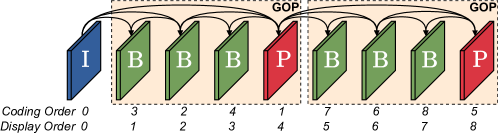
Figure 1: Random Access configuration, GOP size is set to 4 to have concise diagrams.

Let $\left\{\mathbf{x}_{i},i\in\mathbb{N}\right\}$ be a video sequence, each frame $\mathbf{x}_{i}$ being a vector of $C$ color channels of height $H$ and width $W$. Video codecs usually process Groups Of Pictures (GOP) of size $N$, with a regular frame organization. Inside a GOP, all frames are inter-coded and rely on already sent frames called references: B-frames use two references while P-frames use a single one. The first frame of the GOP relies either on a preceding GOP or on an intra-frame (I-frame) denoted as $\mathbf{x}_{0}$. This work primarily targets the Random Access configuration (Fig. 1), because it features I, P and B-frames. Here, we consider the rate-distortion trade-off, weighted by $\lambda$, of a single GOP plus an initial I-frame $\mathbf{x}_{0}$:

$$\mathcal{L}_{\lambda}=\sum_{t=0}^{N}\mathrm{D}(\hat{\mathbf{x}}_{t},\mathbf{x}_{t})+\lambda\mathrm{R}(\hat{\mathbf{x}}_{t}),\text{ with }\mathrm{D}\text{ the MSE and }\mathrm{R}\text{ the rate.}$$ (1)

2.1 B-frame Coding

The proposed architecture processes the entire GOP (I, P and B-frames) using a unique neural-based coder. B-frames coding is detailed here. Thanks to conditional coding, I and P-frames are processed by simply bypassing some steps of the B-frame coding process as explained in Section 2.2.

Let $\mathbf{x}_{t}$ be the current B-frame and $(\hat{\mathbf{x}}_{p},\hat{\mathbf{x}}_{f})$ two reference frames. Figure 2 depicts the coding process of $\mathbf{x}_{t}$. First, $(\mathbf{x}_{t},\hat{\mathbf{x}}_{p},\hat{\mathbf{x}}_{f})$ are fed to MOFNet which computes and conveys—at a rate $R_{m}$—two optical flows $(\mathbf{v}_{p},\mathbf{v}_{f})$, a pixel-wise prediction weighting $\bm{\beta}$ and a pixel-wise coding mode selection $\bm{\alpha}$. The optical flow $\mathbf{v}_{p}$ (respectively $\mathbf{v}_{f}$) represents a 2D pixel-wise motion from $\mathbf{x}_{t}$ to $\hat{\mathbf{x}}_{p}$ (resp. $\hat{\mathbf{x}}_{f}$). It is used to interpolate the reference through a bilinear warping $w$. The pixel-wise weighting $\bm{\beta}$ is applied to obtain the bi-directional weighted prediction $\tilde{\mathbf{x}}_{t}$:

$$\tilde{\mathbf{x}}_{t}=\bm{\beta}\odot w(\hat{\mathbf{x}}_{p};\mathbf{v}_{p})+(1-\bm{\beta})\odot w(\hat{\mathbf{x}}_{f};\mathbf{v}_{f}),\left\{\begin{array}[]{l}\odot\text{ is a pixel-wise multiplication,}\\ \mathbf{v}_{p}\text{ and }\mathbf{v}_{f}\in\mathbb{R}^{2\times H\times W},\ \bm{\beta}\in\left[0,1\right]^{H\times W}\end{array}\right.$$ (2)

The coding mode selection $\bm{\alpha}\in\left[0,1\right]^{H\times W}$ arbitrates between transmission of $\mathbf{x}_{t}$ using CodecNet versus Skip mode, a direct copy of $\tilde{\mathbf{x}}_{t}$. CodecNet sends areas of $\mathbf{x}_{t}$ selected by $\bm{\alpha}$, using information from $\tilde{\mathbf{x}}_{t}$ to reduce its rate $R_{c}$. The total rate required for $\mathbf{x}_{t}$ is $R=R_{m}+R_{c}$ and the decoded frame $\hat{\mathbf{x}}_{t}$ is the sum of both contributions: $\hat{\mathbf{x}}_{t}=\underbrace{(1-\bm{\alpha})\odot\tilde{\mathbf{x}}_{t}}_{\text{Skip}}+\underbrace{c(\bm{\alpha}\odot\mathbf{x}_{t},\bm{\alpha}\odot\tilde{\mathbf{x}}_{t})}_{\text{CodecNet}}$.

2.2 Conditional Coding

Conditional coding (Ladune et al., 2020) allows to exploit decoder-side information more efficiently than residual coding. Its architecture is similar to an auto-encoder (Ballé et al., 2018), with one additional shortcut transform (Fig. 2). It can be understood through the description of its 3 transforms.
Shortcut transform $g^{\prime}_{a}$ (Decoder)—Its role is to extract information from the reference frames available at the decoder (i.e. at no rate). The information is computed as latents $\mathbf{y}^{\prime}$.
Analysis transform $g_{a}$ (Encoder)—It estimates and conveys the information not available at the decoder i.e. the unpredictable part. The information is computed as latents $\hat{\mathbf{y}}$.
Synthesis transform $g_{s}$ (Decoder)—Latents from the analysis and shortcut transforms are concatenated and synthesized to obtain the desired output.

Unlike residual coding, conditional coding leverages decoder-side information in the latent domain. As noted by Djelouah et al. (2019), this makes the system more resilient to the absence of information at the decoder (i.e. for I-frames). Thus, MOFNet and CodecNet implement conditional coding to be able to process I, P and B-frames as well as lowering their rate. I and P-frames are compressed using the B-frames coding scheme, with the same parameters, and ignore the unavailable elements.
I-frame—Motion compensation is not available. As such, MOFNet is ignored, $\bm{\alpha}$ is set to 1 and CodecNet conveys the whole frame, with its shortcut latents $\mathbf{y}^{\prime}_{c}$ set to $0$.
P-frame—Bi-directional motion compensation is not available. $\bm{\beta}$ is set to 1 to only rely on the prediction from $\hat{\mathbf{x}}_{p}$. MOFNet shortcut latents $\mathbf{y}^{\prime}_{m}$ are set to $0$.

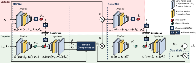
Figure 2: Diagram of the system. A detailed version can be found in appendix D. Arithmetic coding uses hyperpriors (Ballé et al., 2018) omitted for clarity. Attention modules are implemented as proposed by Cheng et al. (2020) and $f=128$. There are 20 millions learnable parameters $\left\{\bm{\phi},\bm{\theta}\right\}$.

3 Training

The training aims at learning to code I, P and B-frames. As such, it considers the smallest coding configuration featuring all 3 types of frame: a GOP of size 2 plus the preceding I-frame. Each training iteration consists in the coding of the 3 frames, followed by a single back-propagation to minimize the rate-distortion cost of equation 1. Unlike previous works, the entire learning process is achieved through this rate-distortion loss. No element of the system requires a pre-training or a dedicated loss term. Moreover, coding the entire GOP in the forward pass enables the system to model the dependencies between coded frames, leading to better coding performance.

The training set is made of 400 000 videos crops of size $256\times 256$, with various resolutions (from 540p to 4K) and framerates (from 24 to 120 fps). The original videos are from several datasets: KonViD-1k (Hosu et al., 2017), CLIC20 P-frame and Youtube-NT (Yang et al., 2020). The batch size is 4 and the learning rate is set to $10^{-4}$ and decreased to $10^{-5}$ during the last epochs. Rate-distortion curves are obtained by training systems for different $\lambda$.

4 Visual Illustrations

This section shows the different quantities at stakes when coding a B-frame $\mathbf{x}_{t}$ (Fig. 3(a)). First, MOFNet outputs two optical flows $(\mathbf{v}_{p},\mathbf{v}_{f})$ (Fig. 3(d)), the prediction weighting $\bm{\beta}$ (Fig. 3(b)) and the coding mode selection $\bm{\alpha}$. The temporal prediction is then computed following equation 2. Most of the time, $\bm{\beta}\simeq 0.5$, mitigating the noise from both bilinear warpings. When the background is disoccluded by a moving object (e.g. the woman), $\bm{\beta}$ equals $0$ on one side of the object and $1$ on the other side. This allows to retrieve the background from where it is available. The competition between Skip mode and CodecNet is weighted by $\bm{\alpha}$. Here, most of $\hat{\mathbf{x}}_{t}$ comes from the Skip mode (Fig. 3(c)). However, the less predictable parts, e.g. the woman, are sent by CodecNet.

To illustrate the conditional coding, $\mathbf{v}_{f}$ is computed by the MOFNet synthesis transform using only the shortcut latents $\mathbf{y}^{\prime}_{m}$ (Fig. 3(e)), the transmitted ones $\hat{\mathbf{y}}_{m}$ (Fig. 3(f)) or both (Fig. 3(d)). The shortcut transform captures the nature of the motion in $\mathbf{y}^{\prime}_{m}$, which allows to synthesize most of $\mathbf{v}_{f}$ without any transmission involved. In contrast, $\hat{\mathbf{y}}_{m}$ consists in a refinement of the flow magnitude. The rate of $\hat{\mathbf{y}}_{m}$ is reduced by using a low spatial resolution, unlike $\mathbf{y}^{\prime}_{m}$ which keeps all the spatial accuracy.

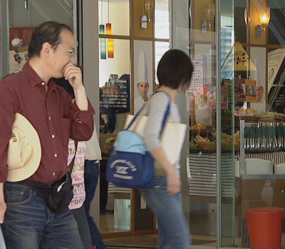
(a) Frame to code $\mathbf{x}_{t}$

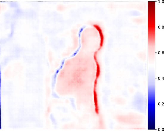
(b) Prediction weighting $\bm{\beta}$

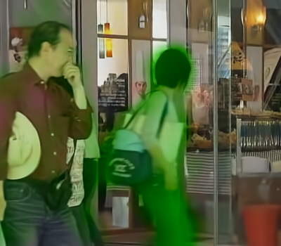
(c) Skip mode $(1-\bm{\alpha})\odot\tilde{\mathbf{x}}_{t}$

(d) Optical flow $\mathbf{v}_{f}$

(e) $\mathbf{v}_{f}$ from $g_{s}(\mathbf{y}^{\prime}_{m};\bm{\theta}_{m})$

(f) $\mathbf{v}_{f}$ from $g_{s}(\hat{\mathbf{y}}_{m};\bm{\theta}_{m})$

Figure 3: B-frame coding from the BQMall sequence featuring moving people on a static background. This crop PSNR is $31.57$ dB, MOFNet rate is $322$ bits and CodecNet rate is $2~{}240$ bits. Second row shows $\mathbf{v}_{f}$ computed by MOFNet synthesis transform from both latents $\texttt{cat}(\hat{\mathbf{y}}_{m},\mathbf{y}^{\prime}_{m})$, from shortcut latents $\mathbf{y}^{\prime}_{m}$ and from the transmitted latent $\hat{\mathbf{y}}_{m}$.

5 Rate-Distortion Results

The proposed system is assessed against x265, an implementation of HEVC. The quality is measured with the PSNR and the BD-rate (Bjontegaard, 2001) indicates the rate difference for the same distortion between two coders. The test sequences are from the HEVC Common Test Conditions (Bossen, 2013). The system flexibility is tested under three coding configurations: All Intra (AI) i.e. coding only the first I-frame, Low-delay P (LDP) i.e. coding one I-frame plus 8 P-frames and Random Access (RA) i.e. coding one I-frame plus a GOP of size 8. BD-rates of the proposed coder against HEVC are presented in the Table 1.

Table 1: BD-rate of the proposed coder against HEVC. Negative results indicate that the proposed coder requires less rate than HEVC for equivalent quality.

Coding configuration	Class (Resolution)					Average
	A (1600p)	B (1080p)	C (480p)	D (240p)	E (720p)
All Intra (AI)	$\mathbf{-11.3}$%	$\mathbf{-9.6}$%	$\mathbf{-14.8}$%	$\mathbf{-45.6}$%	$\mathbf{-25.8}$%	$\mathbf{-21.4}$%
Low-delay P (LDP)	$\mathbf{-4.7}$%	$29.1$%	$14.3$%	$\mathbf{-9.5}$%	$10.0$%	$7.8$%
Random Access (RA)	$5.3$%	$29.9$%	$7.0$%	$\mathbf{-27.2}$%	$\mathbf{-18.7}$%	$\mathbf{-0.7}$%

The proposed system outperforms HEVC in AI configuration, proving that it properly handles I-frames. It is on par with HEVC for RA coding and slightly worse than HEVC for LDP coding. This shows that the same coder is also able to efficiently code P and B-frames, without affecting the I-frames performance. To the best of our knowledge, this is the first system to achieve compelling performance under different coding configurations with a single end-to-end learned coder for the three types of frame.

6 Conclusion

This paper proposes a new framework for end-to-end video coding. It is based on MOFNet and CodecNet, which use conditional coding to leverage the information present at the decoder. Thanks to conditional coding, all types of frame (I, P & B) are processed using the same coder with the same parameters, offering a great flexibility in the coding configuration. The entire training process is performed through the minimization of a unique rate-distortion cost. Its flexibility is illustrated under three coding configurations: All Intra, Low-delay P and Random Access, where the system achieves performance competitive with HEVC.
The main focus of this work is not in the internal design of the networks architecture (MOFNet and CodecNet). Future work will investigate more advanced architectures, from the optical flow estimation or the learned image coding literature, which should bring performance gains.

Appendix A Supplementary Rate-distortion Results

A.1 Sequence-by-sequence BD-rates

Table 2 details the sequence-by-sequence BD-rates that gives the averaged results presented in Table 1. HEVC compression is achieved using ffmpeg with the following command:

ffmpeg -video_size WxH -i in.yuv -c:v libx265 -pix_fmt yuv420p -x265-params "keyint=9:min-keyint=9" -crf QP -preset medium -tune psnr out.mp4

The BD-rate is computed using four quality factors QP $=\left\{27,32,37,42\right\}$. The Low-delay P configuration is obtained by changing the tune option to zerolatency. WxH denotes the video width and height.

Table 2: BD-rate of the proposed coder against HEVC. Negative results indicate that the proposed coder requires less rate than HEVC for equivalent quality.

Class	Sequence name	Coding configuration
(Resolution)		All Intra (AI)	Low-delay P (LDP)	Random Access (RA)
A (1600p)	Traffic	$-13.1$%	$12.8$%	$9.2$%
	PeopleOnStreet	$-18.6$%	$-20.4$%	$-11.4$%
	Nebuta	$-2.6$%	$-18.7$%	$16.8$%
	SteamLocomotive	$-10.8$%	$7.7$%	$6.7$%
Average		$\mathbf{-11.3}$%	$\mathbf{-4.7}$%	$\mathbf{5.3}$%
B (1080p)	Kimono	$-28.7$%	$-1.8$%	$18.5$%
	ParkScene	$-17.0$%	$3.4$%	$4.5$%
	Cactus	$-4.5$%	$6.3$%	$12.7$%
	BQTerrace	$-6.4$%	$86.9$%	$30.6$%
	BasketballDrive	$-4.0$%	$50.6$%	$83.0$%
Average		$\mathbf{-9.6}$%	$\mathbf{29.1}$%	$\mathbf{29.9}$%
C (480p)	RaceHorses	$-22.7$%	$-12.0$%	$16.8$%
	BQMall	$-15.7$%	$20.3$%	$-2.6$%
	PartyScene	$-4.8$%	$38.6$%	$20.0$%
	BasketballDrill	$-25.6$%	$10.4$%	$6.1$%
Average		$\mathbf{-14.8}$%	$\mathbf{14.3}$%	$\mathbf{7.0}$%
D (240p)	RaceHorses	$-50.1$%	$-26.0$%	$-12.1$%
	BQSquare	$-25.2$%	$29.8$%	$-22.4$%
	BlowingBubbles	$-49.4$%	$-22.3$%	$-33.4$%
	BasketballPass	$-57.5$%	$-19.5$%	$-41.1$%
Average		$\mathbf{-45.6}$%	$\mathbf{-9.5}$%	$\mathbf{-27.2}$%
E (720p)	FourPeople	$-25.5$%	$3.8$%	$-20.3$%
	Johnny	$-25.2$%	$15.8$%	$-18.5$%
	KristenAndSara	$-26.6$%	$10.5$%	$-17.3$%
Average		$\mathbf{-25.8}$%	$\mathbf{10.0}$%	$\mathbf{-18.7}$%
All classes average		$\mathbf{-21.4}$%	$\mathbf{7.8}$%	$\mathbf{-0.7}$%

A.2 Supplementary Anchors

Previous work (Lu et al., 2019; Djelouah et al., 2019) uses AVC as an anchor. Table 3 displays the BD-rate of the proposed system against x264 through the following command:

ffmpeg -video_size WxH -i in.yuv -c:v libx264 -pix_fmt yuv420p -g 9 -crf QP -preset medium -tune psnr out.mp4

The proposed system consistently outperforms AVC in all classes under the three coding configurations.

Table 3: BD-rate of the proposed coder against AVC. Negative results indicate that the proposed coder requires less rate than AVC for equivalent quality.

Class	Sequence name	Coding configuration
(Resolution)		All Intra (AI)	Low-delay P (LDP)	Random Access (RA)
A (1600p)	Traffic	$-29.8$%	$-13.5$%	$-16.6$%
	PeopleOnStreet	$-34.4$%	$-32.6$%	$-22.4$%
	Nebuta	$-25.3$%	$-53.2$%	$-17.3$%
	SteamLocomotive	$-27.4$%	$-12.5$%	$-16.4$%
Average		$\mathbf{-29.2}$%	$\mathbf{-27.9}$%	$\mathbf{-18.1}$%
B (1080p)	Kimono	$-40.8$%	$-31.3$%	$-21.0$%
	ParkScene	$-26.3$%	$-10.2$%	$-15.9$%
	Cactus	$-22.3$%	$-15.0$%	$-13.5$%
	BQTerrace	$-16.7$%	$32.2$%	$-4.8$%
	BasketballDrive	$-18.7$%	$-0.8$%	$13.2$%
Average		$\mathbf{-25.0}$%	$\mathbf{-5.0}$%	$\mathbf{-8.4}$%
C (480p)	RaceHorses	$-22.4$%	$-13.2$%	$9.5$%
	BQMall	$-11.2$%	$8.2$%	$-7.0$%
	PartyScene	$3.2$%	$28.7$%	$14.3$%
	BasketballDrill	$-28.9$%	$-19.1$%	$-21.7$%
Average		$\mathbf{-14.8}$%	$\mathbf{1.1}$%	$\mathbf{-1.2}$%
D (240p)	RaceHorses	$-32.9$%	$-18.2$%	$-5.6$%
	BQSquare	$-2.2$%	$42.1$%	$-8.8$%
	BlowingBubbles	$-26.9$%	$-6.1$%	$-21.5$%
	BasketballPass	$-32.3$%	$-8.3$%	$-29.1$%
Average		$\mathbf{-23.6}$%	$\mathbf{2.4}$%	$\mathbf{-15.8}$%
E (720p)	FourPeople	$-28.5$%	$-14.7$%	$-31.5$%
	Johnny	$-27.5$%	$-7.5$%	$-32.8$%
	KristenAndSara	$-29.5$%	$-15.5$%	$-32.5$%
Average		$\mathbf{-28.5}$%	$\mathbf{-12.5}$%	$\mathbf{-32.2}$%
All classes average		$\mathbf{-24.2}$%	$\mathbf{-8.4}$%	$\mathbf{-15.1}$%

Appendix B System Behavior on the FourPeople Sequence

Additional illustrations of the system behavior are given here for the FourPeople sequence, extracted from the HEVC Common Test Conditions. This sequence shows four people slightly moving in front of a still background. The first frame is coded as an I-frame and the next 8 frames are compressed using a (random access) GOP of size 8.

B.1 Rate-distortion curves

Rate-distortion results of the proposed coder against HEVC and AVC are presented in Figure 4. On this sequence, the system significantly outperforms HEVC across the entire rate range.

Figure 4: Rate-distortion curve of the proposed system against AVC and HEVC for the FourPeople sequence. The circled points are used to generate the visual examples.

B.2 Rate Distribution inside a GOP

The Figure 5 exhibits the distribution of the rate and of the PSNR across the frames of a GOP. The PSNR is stable for all the coded frames, ensuring temporal consistency. As their distortion is roughly the same, their rate is function of their predictability. Indeed, the less predictable is a frame, the more information are transmitted. As a result, frames B4 or P8 require more bits to be sent than other inter-frames because their references are temporally further, making them less predictable.

(a) Rate per frame in a GOP.

(b) PSNR per frame in a GOP.

Figure 5: Distribution of the rate and the PSNR across all frames of a GOP. Avg denotes the mean value computed on I-frame and the GOP of size 8.

B.3 Detailed B-frame Coding

This section displays the quantities involved when coding a B-frame $\mathbf{x}_{t}$ (Fig. 6(a)). The two optical flows $\mathbf{v}_{p}$, $\mathbf{v}_{f}$ (Fig. 6(c) and 6(d)) and the pixel-wise bi-directional weighting $\bm{\beta}$ (Fig. 6(f)) are used to compute the temporal prediction $\tilde{\mathbf{x}}_{t}$ as specified in equation 2. Because both flows represent the motion from $\mathbf{x}_{t}$ to a reference, they are activated at the same spatial locations but with different directions, resulting in different visualization colors. Some areas (e.g. the left man’s hand) exhibits a motion which is not well captured by the system, causing checkerboard artifacts in the visualization. Disocclusions occurring due to moving objects are handled using $\bm{\beta}=0$ on one side of the objects and $\bm{\beta}=1$ on the other side. This behavior can be seen around the left man’s arm.

MOFNet also computes and transmits the coding mode selection $\bm{\alpha}$ (Fig. 6(e)). Areas in blue ($\bm{\alpha}=0$) rely on Skip mode to be reconstructed (Fig. 6(h)) while areas in red ($\bm{\alpha}=1$) are transmitted with CodecNet (Fig. 6(g)). Most of the decoded frame (Fig. 6(b)) comes from Skip mode whereas areas transmitted with CodecNet are only those not well predicted enough e.g. the left man’s hand. Skip mode relevance is illustrated through the spatial distribution of CodecNet rate (Fig. 6(i)). Thanks to Skip mode, only few areas of the frame use CodecNet, resulting in few areas for which bits are spent. Lastly, the spatial distribution of MOFNet rate (Fig. 6(j)) shows that all of the coding scheme side-information $(\bm{\alpha},\bm{\beta},\mathbf{v}_{p},\mathbf{v}_{f})$ are transmitted for a low rate.

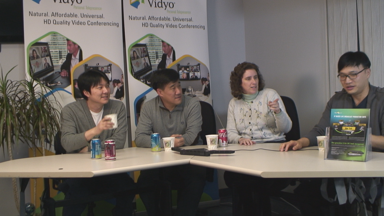
(a) Frame to code $\mathbf{x}_{t}$

(b) Compressed frame $\hat{\mathbf{x}}_{t}$, PSNR is $37.31$ dB

(c) Optical flow $\mathbf{v}_{p}$

(d) Optical flow $\mathbf{v}_{f}$

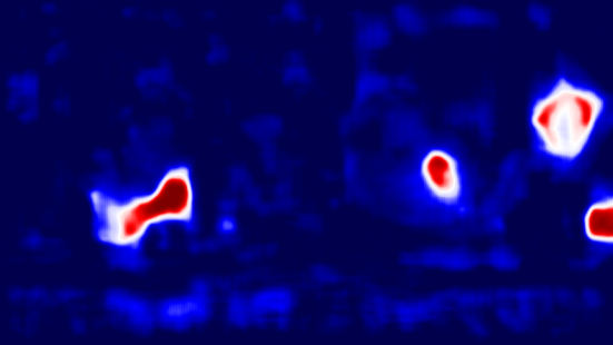
(e) Coding mode $\bm{\alpha}$. Red: CodecNet, blue: Skip

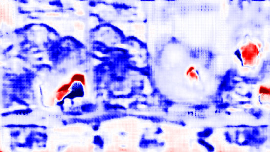
(f) Bi-directional weighting $\bm{\beta}$. Red $=1$, blue $=0$

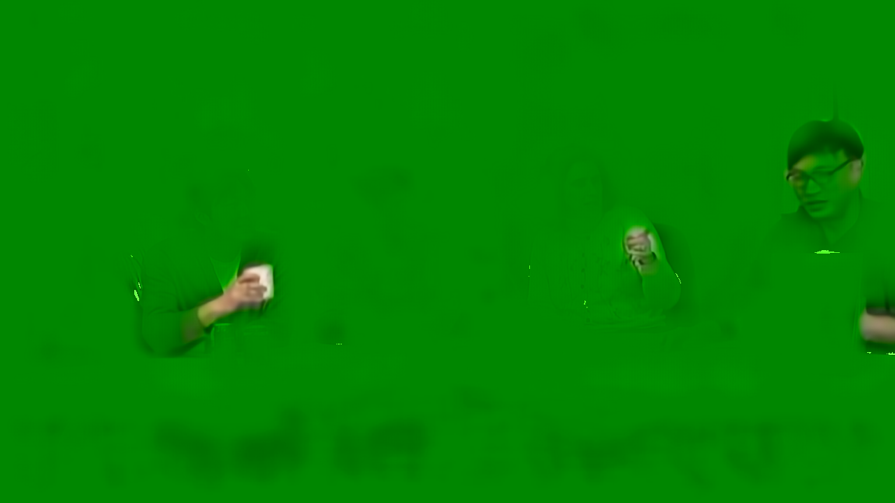
(g) CodecNet part $c(\bm{\alpha}\odot\mathbf{x}_{t},\bm{\alpha}\odot\tilde{\mathbf{x}}_{t})$

(h) Skip part $(1-\bm{\alpha})\odot\tilde{\mathbf{x}}_{t}$

(i) Distribution of CodecNet rate $R_{c}=4~{}332$ bits

(j) Distribution of MOFNet rate $R_{m}=922$ bits

Figure 6: Detailed visualizations for B-frame coding.

B.4 Conditional Coding

Conditional coding relevance is illustrated for CodecNet by synthesizing its output from the shortcut latents only 7(b), the sent latents only 7(c) or both latents 7(a). Similarly to MOFNet, most of CodecNet output is retrieved from the shortcut latents and few information are transmitted, resulting in significant rate savings. The shortcut latents are computed from the temporal prediction $\tilde{\mathbf{x}}_{t}$. Therefore, a poor prediction results in shortcut latents lacking some information, requiring CodecNet to convey something in these areas. Here they correspond to the quickly moving objects such as the people’s hands, whose prediction results from badly estimated flows (Fig. 6(c), 6(d)). This example shows that even with an inaccurate $\tilde{\mathbf{x}}_{t}$, CodecNet exploits all information from $\tilde{\mathbf{x}}_{t}$ and only transmits correction terms to obtain a proper reconstruction.

(a) CodecNet output from both latents: $g_{s}(\texttt{cat}(\hat{\mathbf{y}}_{c},\mathbf{y}_{c}^{\prime});\bm{\theta}_{c})$

(b) CodecNet output from shortcut latents only: $g_{s}(\mathbf{y}_{c}^{\prime};\bm{\theta}_{c})$

(c) CodecNet output from transmitted latents only: $g_{s}(\hat{\mathbf{y}}_{c};\bm{\theta}_{c})$

Figure 7: Illustration of the conditional coding behavior for CodecNet.

B.5 Visual Comparison

The Figure 8 offers a visual comparison of a B-frame, compressed by HEVC and by the proposed system. For a lower rate, the system achieves a higher PSNR than HEVC. The zoom on the man’s hand shows that moving areas are well handled by the system. The high frequencies in the background (the text) are properly recovered. The system obtains a smoother reconstruction with fewer coding artifacts than HEVC, i.e. without blocking or rigging effects.

(a) Original frame

(b) HEVC: PSNR of the GOP is $36.94\text{ dB}$ and the GOP rate is $1.27\text{ Mbit/s}$.

(c) Proposed system: PSNR of the GOP is $37.29\text{ dB}$ and the GOP rate is $1.21\text{ Mbit/s}$.

Figure 8: Visual comparison of a B-frame compression.

Appendix C System Behavior on the BQMall Sequence

The behavior of the proposed system is detailed on the BQMall sequence, extracted from the HEVC Common Test Conditions. This sequence features people walking in front of a static background. In this example, the first frame is coded as an I-frame and the next 8 frames are compressed using a (random access) GOP of size 8. This appendix provides additional illustrations to the ones already shown in section 4.

C.1 Rate-distortion curves

The Figure 9 presents the rate-distortion results of the proposed coder against HEVC and AVC. For this sequence the system outperforms HEVC at low rate. However, the system quality starts saturating at high rate resulting in worse performance than HEVC. We note that the quality saturation issue seems to be inherent to the auto-encoder architecture as noted by Helminger et al. (2020).

Figure 9: Rate-distortion curve of the proposed system against AVC and HEVC for the BQMall sequence. The circled points are used to generate the visual examples.

C.2 Rate Distribution inside a GOP

The Figure 10 presents the distribution of the rate and of the PSNR across the frames of a GOP. Similarly to the FourPeople sequence, the PSNR remains consistent for all the coded frames. Because this sequence is less static than FourPeople, the inter-frame rates are higher.

(a) Rate per frame in a GOP.

(b) PSNR per frame in a GOP.

Figure 10: Distribution of the rate and the PSNR across all frames of a GOP. Avg denotes the mean value computed on the I-frame and the GOP of size 8.

C.3 Visual Comparison

The Figure 11 offers a visual comparison of a B-frame, compressed by HEVC and by the proposed system. At a similar rate, HEVC achieves a better PSNR than the proposed coder and seems to retain more high frequency contents. However, it comes as the cost of significant blocking artifacts and pronounced ringing effects. Due to its convolutional nature, the proposed system offers a smoother output, with fewer compression artifacts.

(a) Original frame

(b) HEVC: The PSNR of the GOP is $33.37\text{ dB}$ and the GOP rate is $1.42\text{ Mbit/s}$.

(c) Proposed system: The PSNR of the GOP is $32.41\text{ dB}$ and the GOP rate is $1.37\text{ Mbit/s}$.

Figure 11: Visual comparison of a B-frame compression.

Appendix D Description of the Network Architecture

The architecture of MOFNet and CodecNet, presented in Figure 2, are described in this appendix.

D.1 Basic Building Blocks

The system uses attention module to increase the capacity of its different transforms. The attention modules are implemented as proposed by Cheng et al. (2020) and are described in Figure 12.

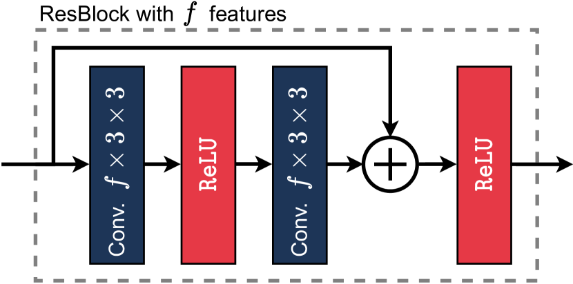
(a) Residual block

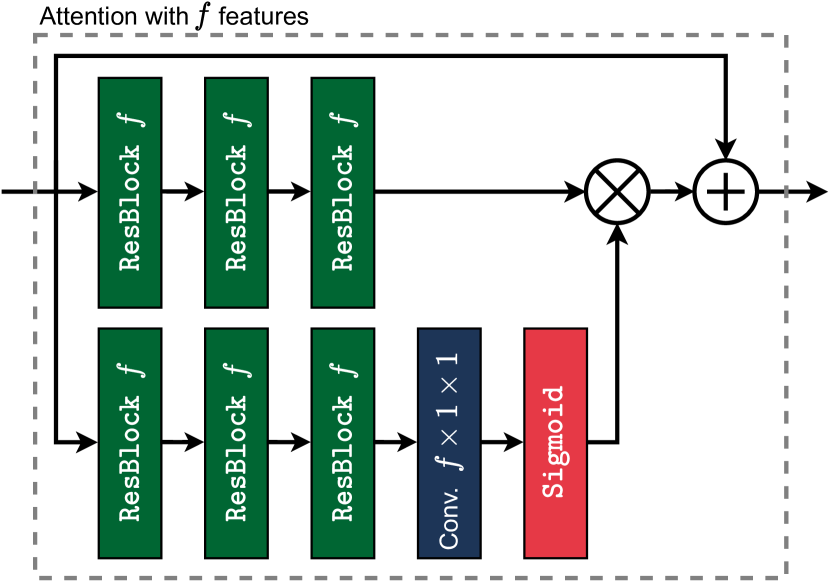
(b) Attention module

Figure 12: Architecture of an attention module. Conv. $f\times k\times k$ denotes a convolutional layer with $f$ output features and a $k\times k$ kernel.

D.2 Hyperprior and Entropy Coding

The transmitted latents of MOFNet and CodecNet are conveyed using entropy coding, which requires an estimate of the latents probability density function (PDF). Each element $\hat{y}_{i}$ of the latents is described by a Laplace PDF, whose parameters $\mu_{i},\sigma_{i}$ are conditioned on a hyperprior $\hat{\mathbf{z}}$ (Ballé et al., 2018). The hyperprior is computed and transmitted from an auxiliary auto-encoder, described in Figure 13(a). The hyperprior transmission uses entropy coding and a Laplace PDF, whose parameters are estimated with an auto-regressive model (see Fig. 13(b)) as proposed by Minnen et al. (2018). Two hyperprior networks are implemented, one for MOFNet and one for CodecNet.

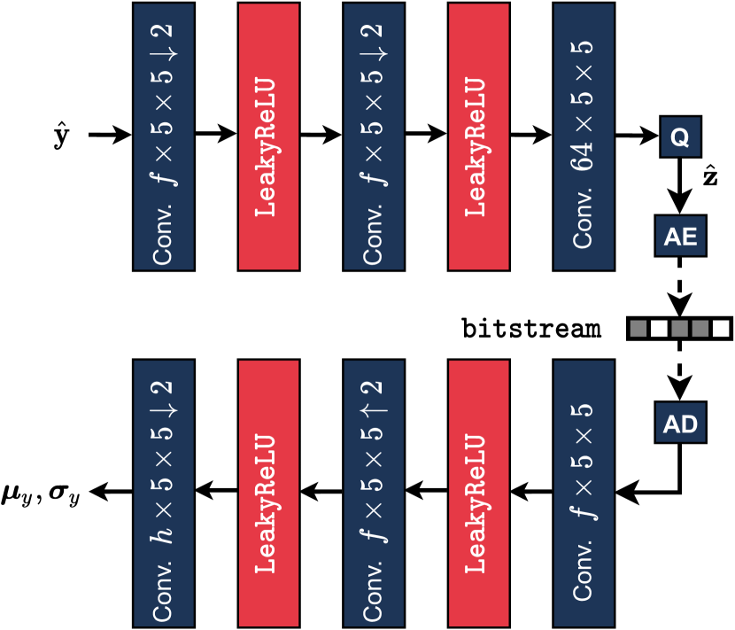
(a) Hyperprior autoencoder

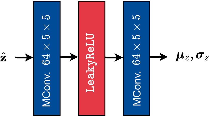
(b) Auto-regressive model.

Figure 13: Architecture of the hyperprior network. $\hat{\mathbf{y}}$ corresponds to MOFNet (sent) latents $\hat{\mathbf{y}}_{m}$ or to CodecNet (sent) latents $\hat{\mathbf{y}}_{c}$. Conv. $f\times k\times k\ \uparrow/\downarrow 2$ denotes a convolutional layer with $f$ output features, a $k\times k$ kernel and a up/down sampling by a factor 2. MConv is a masked convolution.

D.3 MOFNet Architecture

The detailed architecture of the three main transforms of MOFNet (analysis, shortcut and synthesis) is depicted in Figure 14.

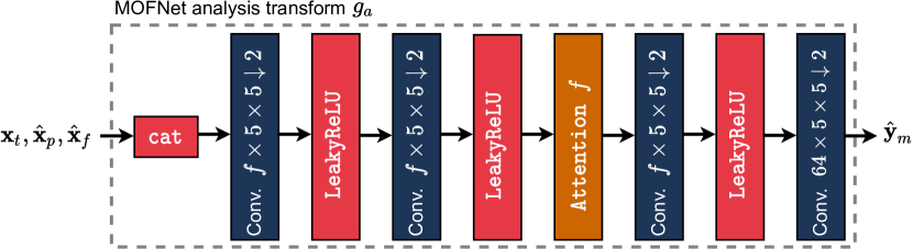
(a) MOFNet analysis transform $g_{a}$

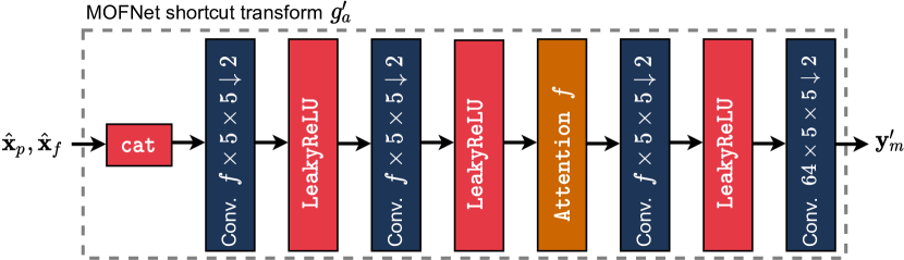
(b) MOFNet shortcut transform $g_{a}^{\prime}$

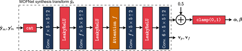
(c) MOFNet synthesis transform $g_{s}$

Figure 14: MOFNet transforms architecture. Conv. $f\times k\times k\ \uparrow/\downarrow 2$ denotes a convolutional layer with $f$ output features, a $k\times k$ kernel and a up/down sampling by a factor 2. $\texttt{Attention}\ f$ is an attention module with $f$ features, cat represents the concatenation along the features dimension and $\texttt{clamp}(0,1)$ is a hard clipping between $0$ and $1$. $f$ is set to 128.

D.4 CodecNet Architecture

The detailed architecture of the three main transforms of CodecNet (analysis, shortcut and synthesis) is depicted in Figure 15.

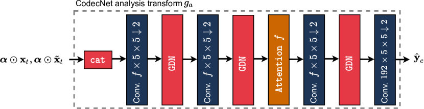
(a) CodecNet analysis transform $g_{a}$

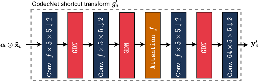
(b) CodecNet shortcut transform $g_{a}^{\prime}$

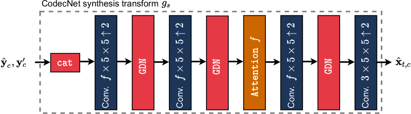
(c) CodecNet synthesis transform $g_{s}$

Figure 15: CodecNet transforms architecture. Conv. $f\times k\times k\ \uparrow/\downarrow 2$ denotes a convolutional layer with $f$ output features, a $k\times k$ kernel and a up/down sampling by a factor 2. $\texttt{Attention}\ f$ is an attention module with $f$ features, cat represents the concatenation along the features dimension. GDN is the General Divisive Normalization introduced by (Ballé et al., 2017). $f$ is set to 128.

References

- Agustsson et al. (2020) Eirikur Agustsson, David Minnen, Nick Johnston, Johannes Balle, Sung Jin Hwang, and George Toderici. Scale-space flow for end-to-end optimized video compression. In Proceedings of the IEEE/CVF Conference on Computer Vision and Pattern Recognition (CVPR), June 2020.
- Ballé et al. (2017) Johannes Ballé, Valero Laparra, and Eero P. Simoncelli. End-to-end optimized image compression. In 5th International Conference on Learning Representations, ICLR 2017, Toulon, France, 2017.
- Ballé et al. (2018) Johannes Ballé, David Minnen, Saurabh Singh, Sung Jin Hwang, and Nick Johnston. Variational image compression with a scale hyperprior. In 6th International Conference on Learning Representations, ICLR 2018, Vancouver, BC, Canada, 2018.
- Bjontegaard (2001) Gisle Bjontegaard. Calculation of average psnr differences between rd-curves. In ITU-T Q.6/16, Doc. VCEG-M33, March 2001.
- Bossen (2013) Frank Bossen. Common test conditions and software reference configurations. In JCTVC-L1100, January 2013.
- Cheng et al. (2020) Zhengxue Cheng, Heming Sun, Masaru Takeuchi, and Jiro Katto. Learned image compression with discretized gaussian mixture likelihoods and attention modules, 2020.
- Djelouah et al. (2019) Abdelaziz Djelouah, Joaquim Campos, Simone Schaub-Meyer, and Christopher Schroers. Neural inter-frame compression for video coding. In 2019 IEEE/CVF International Conference on Computer Vision, ICCV 2019, Seoul, Korea (South), 2019, pp. 6420–6428, 2019. doi: 10.1109/ICCV.2019.00652.
- Helminger et al. (2020) Leonhard Helminger, Abdelaziz Djelouah, Markus Gross, and Christopher Schroers. Lossy image compression with normalizing flows, 2020.
- Hosu et al. (2017) Vlad Hosu, Franz Hahn, Mohsen Jenadeleh, Hanhe Lin, Hui Men, Tamás Szirányi, Shujun Li, and Dietmar Saupe. The konstanz natural video database (konvid-1k). In 2017 Ninth International Conference on Quality of Multimedia Experience (QoMEX), pp. 1–6. IEEE, 2017.
- J. Chen (2020) S. Kim J. Chen, Y. Ye. Algorithm description for versatile video coding and test model 8 (vtm 8), Jan. 2020.
- Ladune et al. (2020) Théo Ladune, Pierrick Philippe, Wassim Hamidouche, Lu Zhang, and Olivier Déforges. Optical flow and mode selection for learning-based video coding. In 2020 IEEE 22nd International Workshop on Multimedia Signal Processing (MMSP), pp. 1–6, 2020. doi: 10.1109/MMSP48831.2020.9287049.
- Liu et al. (2019) Haojie Liu, Han Shen, Lichao Huang, Ming Lu, Tong Chen, and Zhan Ma. Learned video compression via joint spatial-temporal correlation exploration. CoRR, abs/1912.06348, 2019.
- Lu et al. (2019) Guo Lu, Wanli Ouyang, Dong Xu, Xiaoyun Zhang, Chunlei Cai, and Zhiyong Gao. DVC: an end-to-end deep video compression framework. In IEEE Conference on Computer Vision and Pattern Recognition, CVPR 2019, Long Beach, CA, USA, 2019, pp. 11006–11015, 2019. doi: 10.1109/CVPR.2019.01126.
- Minnen et al. (2018) David Minnen, Johannes Ballé, and George Toderici. Joint autoregressive and hierarchical priors for learned image compression. In Conference on Neural Information Processing Systems 2018, NeurIPS,, Montréal, Canada., pp. 10794–10803, 2018.
- Sullivan et al. (2012) Gary J. Sullivan, Jens-Rainer Ohm, Woo-Jin Han, and Thomas Wiegand. Overview of the high efficiency video coding (hevc) standard. IEEE Trans. Cir. and Sys. for Video Technol., 22(12):1649–1668, December 2012. ISSN 1051-8215. doi: 10.1109/TCSVT.2012.2221191.
- Yang et al. (2020) Ruihan Yang, Yibo Yang, Joseph Marino, and Stephan Mandt. Hierarchical autoregressive modeling for neural video compression, 2020.