The X17 boson and the ${{}^{3}{\rm H}}(p,e^{+}e^{-}){{}^{4}{\rm He}}$ and ${{}^{3}{\rm He}}(n,e^{+}e^{-}){{}^{4}{\rm He}}$ processes: a theoretical analysis

Abstract

The present work deals with $e^{+}$-$e^{-}$ pair production in the four-nucleon system. We first analyze the process as a purely electromagnetic one in the context of a state-of-the-art approach to nuclear strong-interaction dynamics and nuclear electromagnetic currents, derived from chiral effective field theory ($\chi$EFT). Next, we examine how the exchange of a hypothetical low-mass boson would impact the cross section for such a process. We consider several possibilities, that this boson is either a scalar, pseudoscalar, vector, or axial particle. The ab initio calculations use exact hyperspherical-harmonics methods to describe the bound state and low-energy spectrum of the $A\,$=$\,4$ continuum, and fully account for initial state interaction effects in the $3+1$ clusters. While electromagnetic interactions are treated to high orders in the chiral expansion, the interactions of the hypothetical boson with nucleons are modeled in leading-order $\chi$EFT (albeit, in some instances, selected subleading contributions are also accounted for). We also provide an overview of possible future experiments probing pair production in the $A\,$=$\,4$ system at a number of candidate facilities.

I Overview

The present work reports on a comprehensive analysis of low-energy $e^{+}$-$e^{-}$ pair production in the four-nucleon system, both as a purely electromagnetic process and by including the contribution of a hypothetical low-mass boson. It is organized as follows. The present section provides an overview of the complete study. Starting from an up-to-date review of the current status of experimental searches and theoretical analyses, we delineate next the chiral-effective-field-theory ($\chi$EFT) framework adopted here to describe nuclear dynamics and to model the interactions of nucleons with the hypothetical boson. We then proceed to a summary of the ab initio predictions obtained for the differential cross sections of the ${{}^{3}{\rm H}}(p,e^{+}e^{-}){{}^{4}{\rm He}}$ and ${{}^{3}{\rm He}}(n,e^{+}e^{-}){{}^{4}{\rm He}}$ reactions. We close with some concluding remarks and a discussion of possible future experiments at a number of candidate facilities. The remaining sections are meant to elaborate more expansively on these various aspects of the calculations.

I.1 Motivation and current status

The possible existence of a new kind of low mass particle (at the MeV scale) is a problem of current and intense theoretical and experimental interest (see, for example, Ref. Battaglieri et al. (2017) and references therein). This interest is, in fact, part of a broader effort aimed at identifying dark matter (DM). Its existence has been postulated to explain a number of gravitational anomalies that have been observed at galactic scales and beyond Bertone and Hooper (2018) since the 1930’s. However, no conclusive experimental signatures of DM have been reported up until now.

A few years ago, there were claims Krasznahorkay et al. (2016) that an unknown particle (denoted as “X17”) had been observed in the process ⁷Li$(p,e^{+}e^{-})^{8}$Be at the ATOMKI experimental facility situated in Debrecen (Hungary). These claims were based on a $\approx 7\sigma$ excess of events in the angular distribution of leptonic pairs produced in this reaction, which has a $Q$-value of about $18$ MeV. The excess—referred to below as the “anomaly”—could be explained by positing the emission of an unknown boson with a mass of about $17$ MeV decaying into $e^{+}e^{-}$ pairs.

The search for bosonic DM candidates had already started several years earlier, by attempting to establish the possible existence of additional forces (beyond gravity), mediated by these bosons Pospelov et al. (2008), between DM and visible matter. To one such class of particles belongs the so-called “dark-photon”, namely a boson of mass $M_{X}$ having the same quantum numbers as the photon, and interacting with a Standard Model (SM) fermion $f$ with a coupling constant given by $\varepsilon\,q_{f}$, where $q_{f}$ is the fermion electric charge. Following several years of experimental searches for dark photons, “exclusion plots” in the $\varepsilon$-$M_{X}$ parameter space were produced, restricting more and more the allowed region Battaglieri et al. (2017); Banerjee et al. (2018). One of the most stringent limits was provided by the NA48/2 experiment, which set $\varepsilon<8\times 10^{-4}$ at $90$% confidence level Batley et al. (2015). Similar limits have been produced by assuming that the X17 is a pseudoscalar particle Andreas et al. (2010), that is, an axion-like particle. More recently, stringent limits were also set by the NA64 experiment at CERN Banerjee et al. (2018). Of course, the analysis becomes more complicated and the ensuing picture far less unambiguous, if the coupling constants are assumed to be different for each of the SM fermions.

The claim of the ${{}^{8}{\rm Be}}$ anomaly by the ATOMKI group Krasznahorkay et al. (2016) soon spurred several theoretical studies. In Ref. Feng et al. (2016), a number of alternatives—that the X17 could be a scalar, a pseudoscalar, or a vector boson—were analyzed. The first two were quickly dismissed, while the possibility that the X17 could be a vector boson, that is, a dark photon, was investigated in detail. In order to circumvent the NA48/2 limit, it was conjectured that the X17 could be “proto-phobic”, namely that it would couple much more weakly to the proton than to the neutron Feng et al. (2016).

Soon after, the possibility that the X17 could be a spin-1 particle interacting via axial couplings to the $u$ and $d$ quarks was explored in Ref. Kozaczuk et al. (2017). In that work, ${{}^{8}{\rm Be}}$ ground- and excited-state wave functions obtained in state-of-the-art shell model calculations were used in combination with the ATOMKI data to constrain the range of X17-quark couplings that could explain the observed anomaly. Limits provided by the bounds determined by a number of other experiments were also analyzed. In case of an axial coupling, the NA48/2 constraint does not apply, but other limits have to be taken into account, for example, from the study of rare $\eta$ and $\phi$ decays and proton fixed target experiments (see, for more details, Ref. Kozaczuk et al. (2017) and references therein).

In 2019, the ATOMKI group reported a similar excess at approximately the same invariant mass in the ${{}^{3}{\rm H}}(p,e^{+}e^{-}){{}^{4}{\rm He}}$ reaction Krasznahorkay et al. (2019); this excess has more recently been confirmed in Ref. Krasznahorkay et al. (2021a). The authors of Ref. Feng et al. (2016) published a new study Feng et al. (2020), considering both the ${{}^{8}{\rm Be}}$ and ${{}^{4}{\rm He}}$ anomalies and allowing for scalar, pseudoscalar, vector, and axial coupling of the X17 to quarks and electrons, with the intent of verifying whether the two results were consistent. They concluded that the “$\,7\sigma$ anomalies reported in [the] ${{}^{8}{\rm Be}}$ and ${{}^{4}{\rm He}}$ nuclear decays are both kinematically and dynamically consistent with the production of a 17 MeV proto-phobic gauge boson” Feng et al. (2020). However, other studies have challenged the explanation of a proto-phobic X17 emission in the ${{}^{8}{\rm Be}}$ experiment, by taking into account existing ${{}^{7}{\rm Li}}(p,\gamma){{}^{8}{\rm Be}}$ cross section data Zhang and Miller (2021); Hayes et al. (2021).

In the following, we consider the more general case of a Yukawa-like interaction between the X17 and a SM fermion of species $f$ (specifically, quarks and electrons) with the coupling constant expressed as $\varepsilon_{f}\,e$, where $e$ ($>0$) is the unit electric charge. The X17 boson must decay promptly in $e^{+}$-$e^{-}$ pairs for these to be detected inside the experimental setup. This observation actually introduces a lower limit to the possible values of $\varepsilon_{e}$. These limits are also established by various electron beam-dump experiments (see, for example, Ref. Andreas et al. (2012) and references therein). For $M_{X}\approx 17$ MeV, the most stringent lower bound, $|\varepsilon_{e}|>2\times 10^{-4}$, comes from the SLAC E141 experiment Riordan et al. (1987), while the upper bound $|\varepsilon_{e}|<2\times 10^{-3}$ has been set by the KLOE-2 experiment Anastasi et al. (2015). See Ref. Kozaczuk et al. (2017) for a comprehensive discussion of these and other constraints regarding $\varepsilon_{e}$.

If the X17 were to couple also to muons, then its existence would have consequences for the well known $(g-2)_{\mu}$ anomaly Abi et al. (2021), namely the discrepancy between the measured and predicted value of the muon anomalous magnetic moment. In this instance, a pure axial coupling to muons would worsen this discrepancy, while a pure vector coupling would reduce it Fayet (2007). Another interesting result comes from new measurements of the fine structure constant using atomic recoil of Rubidium Morel et al. (2020). Using this measurement, the SM prediction for $(g-2)_{e}$ too is in tension with the experimental value (at about $1.6\,\sigma$). Also in this case, a pure vector coupling of the X17 to the electron with $|\varepsilon_{e}|=(8\pm 3)\times 10^{-4}$ Morel et al. (2020) would resolve this tension.

The observation of the ${{}^{8}{\rm Be}}$ and ${{}^{4}{\rm He}}$ anomalies has triggered a rapidly growing number of theoretical studies Zhang and Miller (2017); Ellwanger and Moretti (2016); Dror et al. (2017); Delle Rose et al. (2017, 2019a, 2019b); Alves and Weiner (2018); Alves (2021); Bordes et al. (2019); Nam (2020); Kirpichnikov et al. (2020); Fayet (2021); Hayes et al. (2021), see Ref. Fornal (2017) for a critical review. On the experimental side, there are several experiments (MEGII Baldini et al. (2018), DarkLight Balewski et al. (2014), SHiP Ahdida et al. (2020), and others Battaglieri et al. (2017)) planning specifically to search for such a light boson. In addition, large collaborations, such as BelleII Kou et al. (2019), NA64 Banerjee et al. (2020), and others, are dedicating part of their efforts in an attempt to clarify this issue.

To date, the explanation of the ${{}^{8}{\rm Be}}$ and ${{}^{4}{\rm He}}$ anomalies remains an open problem. If the existence of such a particle were to be experimentally confirmed, it would have profound repercussions for the study of DM and for beyond SM theories. It is worthwhile pointing out here that most theoretical analyses so far have assumed that the reactions proceed via a two step process. First, a resonant state is formed in the collision of the incident nucleon with the target nucleus and, second, this resonant state decays to the ground state by emitting either a photon or the hypothetical X17 boson.

This resonance-saturation approach permits the properties of the X17 particle to be inferred Feng et al. (2016); Kozaczuk et al. (2017); Feng et al. (2020) from the quantum numbers of the decaying and ground states, assuming conservation of parity and other symmetries. While such a treatment may be justified in the case of ${{}^{8}{\rm Be}}$ where the initial state $p+{{}^{7}{\rm Li}}$ populates the (relatively narrow isoscalar and isovector) $1^{+}$ resonances of ${{}^{8}{\rm Be}}$, it becomes problematic in the case of ${{}^{4}{\rm He}}$, since the low-energy $p+{{}^{3}{\rm H}}$ initial states may populate the fairly narrow $0^{+}$ and $0^{-}$ resonances of ${{}^{4}{\rm He}}$. Furthermore, contributions from farther resonances or from direct (non-resonant) capture cannot be excluded a priori, and should be estimated. As a matter of fact, in Ref. Zhang and Miller (2021), the contribution of the direct $p+{{}^{7}{\rm Li}}$ capture in different waves has been found important, if not dominant. For future reference, the low-energy spectrum of ⁴He is reported in Fig. 1. The energies and widths of the various resonances have been determined in R-matrix analyses Tilley et al. (1992).

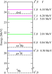
Figure 1: The low-energy spectrum of ⁴He Tilley et al. (1992). The dashed lines indicate the thresholds for the opening of the 1+3 and 2+2 channels, while the solid lines indicate the energies of the various resonances with corresponding widths, $J^{\pi}$, and isospin assignments to the right.

Recently, it was conjectured in Ref. Kálmán and Keszthelyi (2020) that the effect of populating higher excited states might cause peaks in the angular distribution of the final pair, and therefore mimic the resonance-like structure observed in the ³H$(p,e^{+}e^{-})^{4}$He ATOMKI experiment. However, such a conjecture does not seem to be borne out by the present analysis. Instead, our calculations, which are based on a realistic and fully microscopic treatment of nuclear dynamics, indicate the absence of any such structure. In particular, the $J^{\pi}\,$=$\,1^{-}$ scattering state, which plays a dominant role, only yields a smooth behavior in the angular correlation between the leptons, although this correlation appears to be rather sensitive to the low-energy structure of the ${{}^{4}{\rm He}}$ continuum.

In a more recent paper Aleksejevs et al. (2021)—see also Ref. Koch (2021) for a similar study—the possibility that the peak seen in the ${{}^{8}{\rm Be}}$ experiment could be caused by higher-order QED effects, beyond the one-photon-exchange approximation, has been investigated. It has been found that the contribution of these corrections increases with the opening angle $\theta_{ee}$ between the lepton momenta, and could explain the observed behavior of the cross section. We should point out that for the ${{}^{8}{\rm Be}}$ experiment the peak structure was observed around $\theta_{ee}\,$=$\,140^{\circ}$. It is not clear if such an explanation will remain valid in the case of the ${{}^{4}{\rm He}}$ experiment, where a sharper peak is observed at a considerably smaller opening angle, around $110^{\circ}$.

I.2 Interactions and currents

Ab initio studies of few-nucleon dynamics can be carried out nowadays with great accuracy Viviani et al. (2020), not only for bound states but also for the low-energy portion of the continuum spectrum, including the treatment of resonances. This capability and the availability of consistent models of nuclear electroweak currents—that is, electroweak currents constructed consistently with the underlying strong-interaction dynamics—make it possible to almost completely remove uncertainties associated with the nuclear wave functions and/or reaction mechanisms, and therefore to unambiguously interpret the experimental evidence. It is within this context that, in the present paper, we provide fairly complete analyses of the ${{}^{3}{\rm H}}(p,e^{+}e^{-}){{}^{4}{\rm He}}$ and ${{}^{3}{\rm He}}(n,e^{+}e^{-}){{}^{4}{\rm He}}$ processes, with and without the inclusion of the hypothetical X17 boson. Below, we briefly outline the theoretical framework, and refer the reader to the following sections for more extended discussions of various aspects of this framework.

The nuclear Hamiltonian is taken to consist of non-relativistic kinetic energy, and two- and three-nucleon interactions. These interactions are derived from two different versions of chiral effective field theory ($\chi$EFT): one Entem and Machleidt (2003); Machleidt and Entem (2011); Epelbaum et al. (2002) retains only pions and nucleons as degrees of freedom, while the other Piarulli et al. (2016, 2018) also retains $\Delta$-isobars. Both $\chi$EFT versions account for high orders in the chiral expansion, but again differ in that the interactions of Refs. Entem and Machleidt (2003); Machleidt and Entem (2011); Epelbaum et al. (2002) are formulated and regularized in momentum space, while those of Refs. Piarulli et al. (2016, 2018) in coordinate space. As a consequence, the former are strongly non-local in coordinate space.

The low-energy constants (LECs) that characterize the two-nucleon interaction have been determined by fits to the nucleon-nucleon scattering database (up to the pion production threshold), while the LECs in the three-nucleon interaction have been constrained to reproduce selected observables in the three-nucleon sector (see Sec. II). However, the nuclear Hamiltonians resulting from these two different formulations both lead to an excellent description of measured bound-state properties and scattering observables in the three- and four-nucleon systems, including in particular the ⁴He ground-state energy and 3+1 low-energy continuum Viviani et al. (2020), germane to the present endeavor.

Another important aspect of the theoretical framework is the treatment of nuclear electromagnetic currents. These currents have been derived within the two different $\chi$EFT formulations we consider here, namely without Pastore et al. (2008, 2009, 2011); Koelling et al. (2009, 2011); Piarulli et al. (2013) and with Schiavilla et al. (2019) the inclusion of explicit $\Delta$-isobar degrees of freedom. They consist of (i) one-body terms, including relativistic corrections suppressed by two orders in the power counting relative to the leading order; (ii) two-body terms associated with one pion exchange (derived from leading and subleading chiral Lagrangians) as well as pion loops, albeit in the $\Delta$-full $\chi$EFT formulation the contributions of $\Delta$ intermediate states have been ignored in these loops; and (iii) two-body contact terms originating from minimal and non-minimal contact couplings.

The subleading one-pion-exchange and non-minimal contact electromagnetic currents are characterized by a number of unknown LECs that have been fixed by reproducing the experimental values of the two- and three-nucleon magnetic moments and by relying on either resonance saturation for the case of the $\Delta$-less formulation Piarulli et al. (2013) or fits to low-momentum transfer data on the deuteron threshold electrodisintegration cross section at backward angles for the case of the $\Delta$-full formulation Schiavilla et al. (2019).

These interactions and the associated electromagnetic currents lead to predictions for light-nuclei electromagnetic observables, including ground-state magnetic moments, radiative transition rates between low-lying states, and elastic form factors, in very satisfactory agreement with the measured values (for recent reviews, see Bacca and Pastore (2014); Carlson et al. (2015); Marcucci et al. (2016)).

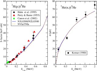
Figure 2: Astrophysical factor for the capture ${{}^{3}{\rm H}}(p,\gamma){{}^{4}{\rm He}}$ (left panel) and total cross section for the capture ${{}^{3}{\rm He}}(n,\gamma){{}^{4}{\rm He}}$ (right panel), calculated in both the $\Delta$-less (N3LO500/N2LO500) and $\Delta$-full (NVIa/3NIa) $\chi$EFT formulations considered in the present work. The experimental data are from Refs. Perry and Bame (1955); Hahn et al. (1995); Canon et al. (2002); Komar et al. (1993).

As an illustration of the validity of the present theoretical framework and the level of sophistication achieved in these ab initio few-nucleon calculations, we present in Fig. 2 predictions for the low-energy radiative captures of protons on ³H and of neutrons on ³He, compared to available experimental data. We use bound and continuum wave functions obtained with hyperspherical-harmonics (HH) methods Kievsky et al. (2008); Marcucci et al. (2020), and fully account in the $n$+³He initial state for its coupling to the energetically open $p$+³H channel. Matrix elements of the (complete) current are calculated with quantum Monte Carlo methods Schiavilla et al. (1989) without any approximations—the statistical errors (not shown in the figure) due to the Monte Carlo integrations are at the % level.

In the energy regime of Fig. 2, these radiative captures proceed primarily via $M_{1}$- and $E_{1}$-transitions between, respectively, the ${}^{3}S_{1}$ and ${}^{1}P_{1}$ incoming states and the ⁴He ground state. We should stress here that in the lepton-pair production processes we consider below, additional $S$- and $P$-wave channels play a prominent role, in particular the ${}^{1}S_{0}$ channel. Lastly, Fig. 2 shows that, at least in the low-energy regime of interest in the present work, the model dependence resulting from the two different $\chi$EFT formulations is weak.

I.3 Including the X17 boson

In the SM and one-photon-exchange approximation, the $e^{+}$-$e^{-}$ pair production on a nucleus is driven by the amplitude (in a schematic notation)

$$T_{fi}=4\pi\alpha\,\frac{(\overline{u}_{-}\,\gamma_{\mu}\,v_{+})\,j^{\mu}_{fi}}{q^{\mu}\,q_{\mu}}\ ,$$ (1)

where $\alpha$ is the fine structure constant, $q^{\mu}$ is the four-momentum transfer defined as the sum of the outgoing-lepton four momenta, $u_{-}$ and $v_{+}$ are, respectively, the electron and positron spinors, and $j^{\mu}_{fi}$ is the matrix element of the nuclear electromagnetic current between the initial and final nuclear states (here, either the $p$+³H or $n$+³He scattering state and ⁴He ground-state); a less cursory description of this as well as the X17-induced amplitudes to follow is provided in Secs. III and V below.

We consider four different possibilities for the coupling of the X17 to electrons and hadrons: scalar ($S$), pseudoscalar ($P$), vector ($V$), and axial ($A$). The electron-X17 interaction Lagrangian density reads

$${\cal L}^{c}_{e,X}(x)=e\,\varepsilon_{e}\,\overline{e}(x)\,\Gamma^{c}\,e(x)\,X_{c}(x)\ ,$$ (2)

where $c$ specifies the nature of the coupling and the associated Lorentz structure,

$$\Gamma^{c=S,P,V,A}=1,i\,\gamma^{5},\gamma^{\mu},\gamma^{\mu}\,\gamma^{5}\ ,$$ (3)

$e(x)$ is the electron field, and $X_{c}(x)\,$=$\,X(x)$ for $c\,$=$\,S,P$ and $X_{c}(x)\,$=$\,X_{\mu}(x)$ for $c\,$=$\,V,A$ represents the X17 field. The single coupling constant $\varepsilon_{e}$ is written in units of the electric charge $e>0$ ($e^{2}\,$=$\,4\pi\alpha$).

The hadron-X17 interaction Lagrangian densities are derived in $\chi$EFT by considering only leading-order contributions (and selected subleading ones in the vector and pseudoscalar cases). A fairly self-contained summary of this derivation is provided in Sec. IV for completeness. Here we write them as

$${\cal L}^{S}_{X}(x)\! = \!e\,\overline{N}(x)[\eta^{S}_{0}+\eta^{S}_{z}\,\tau_{3}]N(x)\,X(x)\ ,$$ (4)

$${\cal L}^{P}_{X}(x)\! = \!e\,\eta_{z}^{P}\,\pi_{3}(x)\,X(x)+e\,\eta^{P}_{0}\overline{N}(x)i\,\gamma^{5}N(x)\,X(x)\ ,$$ (5)

$${\cal L}^{V}_{X}(x)\! = \!e\,\overline{N}(x)[\eta^{V}_{0}+\eta^{V}_{z}\,\tau_{3}]\gamma^{\mu}\,N(x)\,X_{\mu}(x)$$

$$\!+\frac{e}{4\,m_{N}}\,\overline{N}(x)[\kappa_{0}\eta^{V}_{0}+\kappa_{z}\eta^{V}_{z}\tau_{3}]\sigma^{\mu\nu}\,N(x)F^{X}_{\mu\nu}(x)\ ,$$

$${\cal L}^{A}_{X}(x) = \!e\,\overline{N}(x)[\eta^{A}_{0}+\eta^{A}_{z}\,\tau_{3}]\gamma^{\mu}\gamma^{5}\,N(x)\,X_{\mu}(x)\ ,$$ (7)

where $m_{N}$ is the nucleon mass, $N(x)$ is the iso-doublet of nucleon fields, $\pi_{3}(x)$ is the third component of the triplet of pion fields, and $F^{X}_{\mu\nu}(x)\,$=$\,\partial_{\mu}\,X_{\nu}(x)-\partial_{\nu}\,X_{\mu}(x)$ is the X17 field tensor. The combinations of LECs (rescaled by $e$) are lumped into the isoscalar and isovector coupling constants $\eta_{0}^{c}$ and $\eta_{z}^{c}$. In the vector case, we have included also the subleading term proportional to $F^{X}_{\mu\nu}(x)$ and where

$$\kappa_{0}\,=\,\kappa_{p}+\kappa_{n}\ ,\qquad\kappa_{z}\,=\,\kappa_{p}-\kappa_{n}\ ,$$ (8)

$\kappa_{p}$ and $\kappa_{n}$ being the anomalous magnetic moments of the proton and neutron, respectively. In the pseudoscalar case, the leading-order interaction originates from the direct coupling of the X17 to the pion. However, since the associated coupling constant is expected to be suppressed Alves and Weiner (2018); Alves (2021), we have also considered an isoscalar coupling of the X17 to the nucleon, even though it is subleading, at least nominally, in the $\chi$EFT power counting relative to the isovector one. As per the axial case, the tree-level ${\cal L}^{A}_{X}(x)$ contains an additional term of the form $\partial^{\mu}\pi_{3}(x)\,X_{\mu}(x)$, which we have dropped.

The X17-induced amplitude for emission of the $e^{+}$-$e^{-}$ pair is then obtained from

$$T_{fi}^{cX}=4\pi\alpha\,\frac{\varepsilon_{e}\,(\overline{u}_{-}\,\Gamma_{c}\,v_{+})\,j_{fi}^{cX}}{q^{\mu}\,q_{\mu}-M_{X}^{2}}\ ,$$ (9)

where $M_{X}$ is the mass of the X17 particle, and $j^{cX}_{fi}$ represents the matrix element of the nuclear current, including the coupling constants $\eta_{\alpha}^{c}$ associated with the X17 particle. To account for its width $\Gamma_{X}$, we make the replacement

$$M_{X}\longrightarrow M_{X}-i\,\Gamma_{X}/2\ .$$ (10)

At the leading order we are considering here, the nuclear current $j^{cX}({\bf q})$ consists of the sum of one-body terms,

$$j^{cX}({\bf q})=\sum_{i=1}^{A}\,O^{cX}_{i}\,e^{i{\bm{q}}\cdot{\bf r}_{i}}\ ,$$ (11)

where ${\bm{q}}$ is the three-momentum transfer (that is, the sum of the outgoing-lepton momenta), and $O_{i}^{cX}$ involves generally the momentum, spin, and isospin operators of nucleon $i$—the specific operator structure obviously depending on the nature of the coupling assumed for the X17—as well as the coupling constants $\eta_{\alpha}^{c}$. As shown in Fig. 1, the low-energy spectrum of ⁴He consists of fairly narrow resonant states. By varying the energy of the incident beam, it might be possible to predominantly populate a specific resonant state by exploiting the selectivity of the transition operator, and therefore infer the nature—scalar, pseudoscalar, vector, or axial—of the (hypothetical ) X17 particle.

I.4 ${{}^{3}{\rm H}}(p,e^{+}e^{-}){{}^{4}{\rm He}}$ and ${{}^{3}{\rm He}}(n,e^{+}e^{-}){{}^{4}{\rm He}}$ cross sections

The amplitudes $T_{fi}$ and $T^{cX}_{fi}$ generally interfere (except when the X17 is a pseudoscalar particle) and the resulting cross section has a complicated structure; it is derived in Sec. VI. In the laboratory frame, the initial state consists of an incoming proton or neutron of momentum ${{\bm{p}}}$ and spin projection $m_{1}$, and a bound ³H or ³He cluster in spin state $m_{3}$ at rest. Its wave function $\Psi_{m_{3},m_{1}}^{(\gamma)}({\bm{p}})$ is such that, in the asymptotic region of large separation ${\bm{y}}_{\ell}$ between the isolated nucleon (particle $\ell$) and the trinucleon cluster (particles $ijk$), it reduces to

$$\Psi_{m_{3},m_{1}}^{(\gamma)}({\bm{p}})\longrightarrow{1\over\sqrt{4}}\sum_{\ell=1}^{4}\phi^{m_{3}}_{\gamma}(ijk)\chi^{m_{1}}_{\gamma}(\ell)\,\Phi_{{\bm{p}}}^{(\gamma)}({\bm{y}}_{\ell})\ ,$$ (12)

where $\Phi_{{\bm{p}}}^{(\gamma)}({\bm{y}}_{\ell})$ is either a Coulomb distorted wave or simply the plane wave $e^{i{{\bm{p}}}\cdot{{\bm{y}}_{\ell}}}$ depending on whether we are dealing with the $p+^{3}$H ($\gamma\,$=$\,1$) or $n+^{3}$He ($\gamma\,$=$\,2$) state. The final state consists of the lepton pair—with the $e^{-}$ having momentum (energy) ${\bm{k}}$ ($\epsilon$) and spin $s$, and the $e^{+}$ having momentum (energy) ${\bm{k}}^{\prime}$ ($\epsilon^{\prime}$) and spin $s^{\prime}$—and the ⁴He ground state recoiling with momentum ${\bm{p}}-{\bm{k}}-{\bm{k}}^{\prime}$. Energy conservation requires

$$\epsilon+\epsilon^{\prime}+\frac{({\bm{p}}-{\bm{k}}-{\bm{k}}^{\prime})^{2}}{2\,M}=E_{0}\ ,$$ (13)

where $M$ is the rest mass of the ⁴He ground state. Further, we have defined $E_{0}=T_{p}+B_{4}-B_{3}\approx 20\,$ MeV, where $T_{p}$ is the kinetic energy of the incident nucleon, and $B_{3}$ and $B_{4}$ are the binding energies of, respectively, the bound three-nucleon cluster and ⁴He.

After integrating out the energy and momentum $\delta$-functions, the five-fold differential cross section, averaged over the azimuthal quantum numbers $m_{1}$ and $m_{3}$ of the nuclear clusters, and summed over the spins of the final leptons, has generally the form

$$\frac{d^{5}\sigma^{(\gamma)}}{d\epsilon\,d\hat{{\bm{k}}}\,d\hat{{\bm{k}}}^{\prime}}\!=\!\sigma^{(\gamma)}(\epsilon,\hat{{\bm{k}}},\hat{{\bm{k}}}^{\prime})+\sigma^{(\gamma)}_{X}(\epsilon,\hat{{\bm{k}}},\hat{{\bm{k}}}^{\prime})+\sigma_{XX}^{(\gamma)}(\epsilon,\hat{{\bm{k}}},\hat{{\bm{k}}}^{\prime})\ ,$$ (14)

where $\sigma^{(\gamma)}$, $\sigma_{X}^{(\gamma)}$, and $\sigma_{XX}^{(\gamma)}$ denote the contributions coming solely from electromagnetic currents, the interference between electromagnetic and X17-induced currents, and purely X17-induced currents, respectively, and $\hat{{\bm{k}}}$ and $\hat{{\bm{k}}}^{\prime}$ specify the directions of the electron and positron momenta. The positron energy $\epsilon^{\prime}$ is fixed by energy conservation, while the electron energy $\epsilon$ is restricted to the range $m_{e}\leq\epsilon\leq\epsilon_{max}$, where the maximum allowed energy $\epsilon_{max}$ is obtained from the solution of Eq. (13) corresponding to a vanishing positron momentum; in fact, since the kinetic energy of the recoiling ⁴He is tiny, $\epsilon_{max}$ is close to $E_{0}-m_{e}$. In the laboratory coordinate system, where the $z$-axis is oriented along the incident beam momentum ${\bm{p}}$, the spherical angles specifying the $\hat{\bm{k}}$ ($\hat{\bm{k}}^{\prime}$) direction are denoted as $\theta$ and $\phi$ ($\theta^{\prime}$ and $\phi^{\prime}$), and

$$\hat{\bm{k}}\cdot\hat{\bm{k}}^{\prime}\equiv\cos\theta_{ee}=\cos\theta\cos\theta^{\prime}+\sin\theta\sin\theta^{\prime}\cos(\phi^{\prime}-\phi)\ .$$ (15)

Of course, the numerical results presented below for the various cross sections depend on the mass $M_{X}$ and width $\Gamma_{X}$ as well as on the values of the coupling constants $\varepsilon_{e}$ and $\eta_{\alpha}^{c}$ of the X17 particle to electrons and hadrons, respectively. We report these and, in particular, the values we have adopted for the LECs entering the combinations $\eta_{\alpha}^{c}$ in Sec. VII. It is important to stress, though, that in this first exploratory study, we are not interested in determining precisely these various parameters (as well as their associated uncertainties), also in view of the fact that the experimental evidence for the existence of the X17 boson is yet to be confirmed unambiguously. Rather, our intent here is (i) to setup the theoretical framework, and (ii) to investigate possible experimental signatures of the X17, in particular, by establishing how its nature affects the behavior of the cross section as function of the energy and lepton angles.

I.4.1 Numerical results: energy dependence

We assume the width of the X17 to come from its decay into $e^{+}$-$e^{-}$ pairs (the branching ratio for decay in a channel other than $e^{+}$-$e^{-}$, such as $\gamma\gamma$ or neutrinos, is estimated to be negligible Feng et al. (2016); Delle Rose et al. (2019b)). This width is seen to scale as $\Gamma^{c}_{X}\sim x_{c}\,\alpha\,\varepsilon_{e}^{2}\,M_{X}$ with a numerical factor $x_{c}$ of order unity—its precise value depending on the assumed coupling between the X17 and the electron. Current bounds indicate $|\varepsilon_{e}|\lesssim 10^{-3}$, and therefore the expected width is of the order of the eV or less, tiny relative to the typical energies of the emitted electrons in the pair production process.

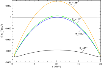
Figure 3: Quantity $Q^{2}-M_{X}^{2}$ as function of the electron energy $\epsilon$ for the configuration in which the lepton pair is produced in a plane orthogonal to the initial proton momentum of energy 0.90 MeV, and for various values of $\theta_{ee}$; here, $M_{X}\,$=$\,17$ MeV. Note that for $\theta_{ee}<112^{\circ}$, the quantity $Q^{2}-M_{X}^{2}$ is always negative.

As is apparent from Eq. (9), the cross section is most sensitive to the X17 presence for momentum transfers $Q^{2}=q^{\mu}q_{\mu}$ such that $Q^{2}\approx M_{X}^{2}$. For the kinematical configuration corresponding to the electron and positron being emitted in the plane perpendicular to the proton momentum (to be specific, we are considering the ³H$(p,e^{+}e^{-})^{4}$He process in the setup of the ATOMKI experiment here), there is a critical angle $\theta^{*}_{ee}\approx 112^{\circ}$, such that for $\theta_{ee}>\theta^{*}_{ee}$ there are two electron energies $\epsilon_{1}$ and $\epsilon_{2}$ that satisfy the condition above, see Fig. 3. For energies close to $\epsilon_{i}$, we can approximate $Q^{2}-M_{X}^{2}\approx\alpha_{i}\,(\epsilon-\epsilon_{i})$, and the X17 propagator—rather, its magnitude square—as

$${1\over|Q^{2}-(M_{X}-i\Gamma_{X}/2)^{2}|^{2}}\approx{\alpha_{i}^{-2}\over(\epsilon-\epsilon_{i})^{2}+(M_{X}\Gamma_{X}/\alpha_{i})^{2}}\ ,$$ (16)

namely a Lorentzian with a width given by $M_{X}\Gamma_{X}/|\alpha_{i}|$. While this width is magnified by the factor $M_{X}|\alpha_{i}|^{-1}$, it is still found to be tiny in comparison to typical $\epsilon_{i}$ values.

Such a narrow width makes it very difficult to reveal the interplay between the electromagnetic and X17-induced amplitudes, in particular to disentangle their interference. However, the experiment has a finite energy resolution, and folding this resolution with the calculated cross sections corresponding to the X17 theoretical width results in a broadening of the peaks.

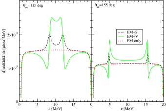
Figure 4: The five-fold differential cross section for the process ${{}^{3}{\rm H}}(p,e^{-}e^{+}){{}^{4}{\rm He}}$ in the ATOMKI setup as function of the electron energy, for the configuration in which the $e^{+}$ and $e^{-}$ momenta are at angles $\theta_{ee}$ of 115^∘ (left panel) and 155^∘ (right panel) between them. The (red) dotted curve represents the results obtained by including the electromagnetic contribution only; the (green) solid curve and (black) dashed curves represent the results obtained by including a X17 boson interacting via a vector and scalar coupling, respectively. Here $M_{X}\,$=$\,17$ MeV and $\Gamma^{\rm eff}\,$=$\,0.4$ MeV, see text for further explanations. The calculations are based on the N3LO500/N2LO500 interactions and accompanying electromagnetic currents.

For the sake of illustration, in Fig. 4 we show the five-fold differential cross section for the process ${{}^{3}{\rm H}}(p,e^{+}e^{-}){{}^{4}{\rm He}}$ as function of the electron energy in the ATOMKI setup (with proton energy of 0.90 MeV) for an effective, albeit perhaps unrealistic, width $\Gamma^{\rm eff}_{X}\,$=$\,0.4$ MeV. In the figure, we have reported the results obtained at angles $\theta_{ee}$ of 115^∘ (left panel) and 155^∘ (right panel), where the condition $Q^{2}$=$\,M^{2}_{X}$ is verified for two energies. The (red) dotted curve represents the results obtained by including only electromagnetic contributions; the (green) solid and (black) dashed curves include the contribution of the X17 particle interacting with nucleons either via a proto-phobic vector or a scalar coupling. We have taken $M_{X}\,$=$\,17$ MeV with the remaining coupling constants chosen arbitrarily.

By inspecting the figure, we see that there is a strong interference between the electromagnetic and vector X17-induced amplitudes. This interference is weaker for the case of a scalar X17. The energy dependence of the differential cross section for pseudoscalar and axial couplings is similar to that obtained for the scalar coupling, and the corresponding results are not shown in Fig. 4; in particular, for a pseudoscalar exchange, the interference (between electromagnetic and X17-induced amplitudes) vanishes identically. Unfortunately, at angles $\theta_{ee}\gtrsim 110^{\circ}$ the differential cross section is rather small (of the order of pb): its accurate measurement would be experimentally very challenging.

I.4.2 Numerical results: angular correlations

In order to compare with the ATOMKI data for the ${{}^{3}{\rm H}}(p,e^{-}e^{+}){{}^{4}{\rm He}}$ reaction reported in Ref. Krasznahorkay et al. (2019), we consider the four-fold differential cross sections obtained by integrating over the electron energy, with the remaining kinematical variables in the same configuration above (that is, the momenta of the lepton pair in the plane orthogonal to the incident proton momentum). Since the ATOMKI cross section measurements are unnormalized, we rescale them to match the calculated values for $\theta_{ee}\lesssim 90^{\circ}$, where the cross section is dominated by the purely electromagnetic amplitude. In the more recent Ref. Krasznahorkay et al. (2021a), “background-free” ${{}^{3}{\rm H}}(p,e^{-}e^{+}){{}^{4}{\rm He}}$ reaction data are also reported, obtained by subtracting the counting rate due to “external” pair conversion (EPC) processes. This EPC rate is estimated on the basis of a GEANT simulation of the processes where real photons emitted in the ${{}^{3}{\rm H}}(p,\gamma){{}^{4}{\rm He}}$ radiative capture convert in lepton pairs by interacting with the experimental apparatus Krasznahorkay et al. (2021a). However, these data at angles $\lesssim 90^{\circ}$ have large errors, making the matching between theory and experiment in this angular range rather problematic. It is for this reason that, in this section, we compare with the (un-subtracted) data of Ref. Krasznahorkay et al. (2019) (qualitatively similar to the un-subtracted data reported in the 2021 study), where errors at angles $\lesssim 90^{\circ}$ are much smaller.

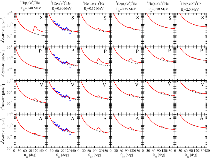
Figure 5: The four-fold differential cross section for the ${{}^{3}{\rm H}}(p,e^{-}e^{+}){{}^{4}{\rm He}}$ and ³He$(n,e^{-}e^{+}){{}^{4}{\rm He}}$ processes at six different incident nucleon energies for the configuration in which the $e^{+}$ and $e^{-}$ momenta are in the plane orthogonal to the incident nucleon momentum and as function of the angle $\theta_{ee}$ between them. The panels labeled S, P, V, and A show the results obtained by including the exchange of a scalar, pseudoscalar, vector, and axial X17, respectively. In all cases, we have taken $M_{X}\,$=$\,17$ MeV and $\Gamma_{X}\,$ as given from the X17 decay in $e^{-}e^{+}$, and have adjusted the coupling constants so as to reproduce the ATOMKI ${{}^{3}{\rm H}}(p,e^{-}e^{+}){{}^{4}{\rm He}}$ cross section data of Ref. Krasznahorkay et al. (2019) at the incident proton energy of 0.90 MeV (see text for further explanations). The dashed (black) and solid (red) curves show the results obtained by including the electromagnetic only or both the electromagnetic and X17 amplitudes. The calculations are based on the N3LO500/N2LO500 interactions and accompanying electromagnetic currents.

We report the calculated cross sections for both ${{}^{3}{\rm H}}(p,e^{+}e^{-}){{}^{4}{\rm He}}$ and ³He$(n,e^{+}e^{-}){{}^{4}{\rm He}}$ reactions at a number of incident proton and neutron energies in Fig. 5. In computing the cross sections, we have taken the width $\Gamma_{X}$ from the X17 decay into $e^{+}$-$e^{-}$ pairs; however, we have folded the resulting calculated values with a Gaussian, in order to account for the finite angular resolution (see Sec. VII). For each of the assumed couplings, we constrain the combinations $\eta^{c}_{\alpha}$ by fitting the ATOMKI data (solid points with the error bars) obtained at an incident proton energy of 0.9 MeV and in the range $\theta_{ee}>90^{\circ}$, where the (purported) X17 signal has been observed (we take as before $M_{X}\,$=$\,17$ MeV). The extracted values of the coupling constants are reported in Sec. VII.2: they depend on the parameters chosen to perform the angular smearing of the theoretical cross sections, and on the factor used to rescale the Atomki data. We anticipate here that both the ${{}^{8}{\rm Be}}$ and ${{}^{4}{\rm He}}$ anomalies can be consistently explained by the hypothesis of a vector X17, while for an axial X17 the coupling constants are found to be seemingly inconsistent with each other. For the scalar and pseudoscalar case it is more difficult to draw any firm conclusion. This issue is discussed in more detail in Sec. VII.2.

In Fig. 5, the incident proton energies of 0.40 and 0.90 MeV correspond to energies $E_{0}$ in Eq. (13) of 20.12 and 20.50 MeV, respectively. Referring to Fig. 1, we see that the lower 20.12 MeV corresponds to the energy of the first $0^{+}$ excited state, while the higher 20.50 MeV (the energy selected in the ATOMKI experiment) is just below the $n+{{}^{3}{\rm He}}$ threshold. The incident neutron energies of 0.17, 0.35, 0.70, and 2.0 MeV correspond to $E_{0}$ values of 20.69, 20.82, 21.08, and 22.08 MeV, and the first three are close to the energy of the $0^{-}$ excited state, while the last is on top of the $2^{-}$ excited state.

This structure of the ⁴He low-energy spectrum and the selectivity of the X17-induced transition operator are reflected in the results of Fig. 5. Referring to Eq. (11) and setting aside the isospin dependence generally of the form $\eta^{c}_{0}+\eta^{c}_{z}\,\tau_{i,z}$, the operator structure $O^{cX}_{i}$ is: 1 (proportional to ${\bm{q}}\cdot{\bm{\sigma}}_{i}$) for a $S$ ($P$) boson exchange and 1 (${\bm{p}}_{i}\cdot{\bm{\sigma}}_{i}$) for the time component and ${\bm{p}}_{i}$ or ${\bm{q}}\times{\bm{\sigma}}_{i}$ (${\bm{\sigma}}_{i}$) for a $V$ ($A$) boson exchange. The $S$ operator (specifically, its isoscalar component) connects the (predominantly isoscalar) $J^{\pi}\,$=$\,0^{+}$ resonance to the ⁴He ground state. This transition is responsible for the prominent low-energy peak seen in Fig. 5; this peak rapidly fades away as the energy of the incident proton increases in the ${{}^{3}{\rm H}}(p,e^{-}e^{+}){{}^{4}{\rm He}}$ process. It is barely visible in the ³He$(n,e^{-}e^{+}){{}^{4}{\rm He}}$ process, since the $n\,+^{3}$He threshold is already relatively far away from the $0^{+}$ resonance energy, see Fig. 1.

Since the purely isovector (pion-mediated) $P$ transition operator has a small matrix element between the (predominantly $T\,$=$\,0$) $0^{-}$ resonance and ⁴He ($0^{+}$) ground state, we have ignored it altogether in the panels of Fig. 5 by setting $\eta^{P}_{z}\,$=$\,0$—that is, by assuming a “piophobic” X17—and have instead considered only the contribution from the isoscalar $P$ transition operator, which has a large matrix element between these $0^{-}$ and $0^{+}$ states. As a consequence, a pronounced peak structure is seen when the energy approaches that of the $0^{-}$ resonance. As this energy increases well beyond the $n+{{}^{3}{\rm He}}$ threshold, additional significant contributions also come from the (relatively broad) $2^{-}$ resonances.

The time component of the $V$ operator has the same structure as the $S$ operator. Its space component, however, produces large electric dipole ($E_{1}$) matrix elements between the $1^{-}$ scattering state and ${{}^{4}{\rm He}}$ ground state (note in Fig. 1 the two wide $1^{-}$ resonances located at energies close to the $d+d$ threshold). These $E_{1}$ matrix elements are found to be much larger than the matrix elements due to the $0^{+}\longrightarrow 0^{+}$ transition, and are the same for both photon and X17-induced amplitudes (modulo coupling constants, of course), see also Ref. Zhang and Miller (2021) for a similar finding in connection with the ${{}^{8}{\rm Be}}$ experiment. Once the values of $\eta^{V}_{0}$ and $\eta^{V}_{z}$ have been constrained to reproduce the ATOMKI data, the height of the peak in the full cross section is nearly constant relative to that in the purely electromagnetic cross section for all energies considered in this work. By contrast, the $1^{+}$ scattering-state contributions are suppressed since they have magnetic-dipole ($M_{1}$) character. Moreover and most importantly, in this ${}^{3}S_{1}$ wave the Pauli principle prevents the four nucleons from coming close together. Even though there are well defined and fairly narrow $2^{-}$ resonances, the associated transitions, having $M_{2}$ character, are suppressed.

The time component of the $A$ operator, which now has both isoscalar and isovector terms, induces big matrix elements between the $0^{-}$ scattering state and ${{}^{4}{\rm He}}$ ground state. In fact, this transition yields the dominant contribution, since now the $1^{-}\longrightarrow 0^{+}$ transition is $M_{1}$ and therefore suppressed by $q$ relative to the $0^{-}\longrightarrow 0^{+}$ one above. The $1^{+}\longrightarrow 0^{+}$ transition is $E_{1}$, but again inhibited by the Pauli repulsion. As a consequence, in the axial case the X17 peak is more pronounced for energies at which the $0^{-}$ state is populated, as for the $P$ case. However, it should be noted that for large angles $\theta_{ee}$ (close to back-to-back configurations), the cross-section enhancement from $A$ couplings is much reduced, due to the vanishing of the X17 $\rightarrow e^{-}e^{+}$ amplitude.

Next, we explore the dependence of the four-fold differential cross sections as function of the polar angles $\theta$ and $\theta^{\prime}$ formed by the directions of the lepton momenta with respect to the incident beam momentum ${\bm{p}}$. We only consider configurations where $\theta\,$=$\,\theta^{\prime}$. The condition $Q^{2}=M_{X}^{2}$ is found to be satisfied for $55^{\circ}<\theta<125^{\circ}$ ($M_{X}=17$ MeV). Therefore, outside this range the X17 peaks do not appear in the cross section. Furthermore, moving away from $\theta\,$=$\,90^{\circ}$, the difference $\Delta\phi=\phi^{\prime}-\phi$ for which the condition $Q^{2}-M_{X}^{2}=0$ is verified, tends to increase, while the values of the parameters $|\alpha_{i}|$ in the expansion of the X17 propagator tend to decrease. One would therefore expect the X17 peak to be located at larger and larger values of $\Delta\phi$, and its height to increase as $|\alpha_{i}|^{-1}$, see Eq. (16).

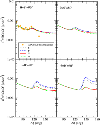
Figure 6: The four-fold differential cross section for the ${{}^{3}{\rm H}}(p,e^{-}e^{+}){{}^{4}{\rm He}}$ process at 0.90 MeV incident proton energy for the configuration in which the $e^{+}$ and $e^{-}$ momenta are emitted at angles $\theta\,$=$\,\theta^{\prime}$ with respect to the incident proton momentum, and as function of the difference $\Delta\phi=\phi^{\prime}-\phi$. The curves labeled S, P, V, and A show the results obtained by including the exchange of a scalar, pseudoscalar, vector, and axial X17, respectively. In all cases, we have taken $M_{X}\,$=$\,17$ MeV and $\Gamma_{X}$ from the decay in $e^{-}e^{+}$, and have adjusted the coupling constants so as to reproduce the ATOMKI ${{}^{3}{\rm H}}(p,e^{-}e^{+}){{}^{4}{\rm He}}$ data Krasznahorkay et al. (2019) at $\theta\,$=$\,\theta^{\prime}\,$=$\,90^{\circ}$, rescaled as discussed in the main text.

The calculations are based on the N3LO500/N2LO500 interactions and accompanying electromagnetic currents.

These expectations are generally borne out by the actual calculations, as shown in Fig. 6. There is a clear dependence on the assumed nature of the X17 boson. It is worthwhile pointing out that for the pseudoscalar case, the larger increase observed in the cross section for $\theta\,$=$\,\theta^{\prime}\,$=$\,60^{\circ}$ comes from a kinematically enhanced contribution of the charge multipole connecting the $2^{-}$ and $0^{+}$ (⁴He) states. For the scalar case, the similar enhancement is due to the contribution of the charge multipole connecting the $1^{-}$ and $0^{+}$ states. Furthermore, we note that in the pseudoscalar (scalar) case the cross section increases (decreases) when $\theta=\theta^{\prime}>90^{\circ}$. This amplifies the differences between the two cases.

I.5 Experimental perspective

The experimental study of the ${{}^{3}{\rm H}}(p,e^{+}e^{-}){{}^{4}{\rm He}}$ reaction performed by the ATOMKI group seems to indicate the existence of a X17 boson. However, it is difficult to establish its quantum numbers, since the data were limited to a few proton energies and only leptons emitted in the plane orthogonal to the beam line were detected. Furthermore, under certain conditions the data may be consistent with standard electromagnetic processes alone Aleksejevs et al. (2021), without the need for invoking the creation of a new particle.

In order to clarify the current ambiguous state of affairs, our calculations suggest to perform an experimental study that covers a wide range in angle and energy, to fully scan the $0^{+}$, $0^{-}$, $2^{-}$, $1^{-}$ excited levels shown in Fig. 1. Such a study would allow us to either confirm or exclude the existence of the X17, and ultimately study its properties, if its existence were to be corroborated. Although the excess of pair-production events as a function of the energy depends on the X17 quantum numbers (i.e., on the nature of its coupling to electrons and nucleons), an experimental setup in which only particles orthogonal to the beam axis are detected might be hindering our ability to discriminate among these different quantum numbers, and hence uniquely identify the X17 properties. This limitation can be appreciated by inspecting Fig. 5, where the predicted trend of the excess is found to be quite similar for the pseudoscalar and axial cases. However, as shown in Fig. 6, the use of a detector with a large angular acceptance would make it possible to discriminate among different options since the angular distribution of the emitted pair depends appreciably on the X17 quantum numbers (a comprehensive analysis of different kinematical configurations will be reported in a future publication). A dedicated detector could also provide a measurement of the pair four-momenta as well as particle identification, to ascertain that the pair is truly an $e^{+}e^{-}$ one.

A prerequisite to realize such a program is the availability of high intensity proton and neutron beams. Concerning the ${{}^{3}{\rm H}}(p,e^{+}e^{-}){{}^{4}{\rm He}}$ reaction, a promising facility is the LUNA-MV accelerator that will soon be operative at the underground Gran Sasso Laboratory (LNGS). At the LNGS the cosmic ray induced background is many orders of magnitude lower than at overground facilities, and the proton beam intensity is a factor hundred higher than at the ATOMKI facility. Thus, LUNA-MV is well suited to perform accurate measurements in the proton energy range approximately ($0.2$–$1.0$) MeV, and in a relatively short time. In this energy range lies the $0^{+}$ resonance located $0.50$ MeV above the $p+^{3}$H threshold. The maximal proton energy is determined by the onset of the huge production of neutrons due to the charge exchange reaction ³H$(p,n)^{3}$He for proton energy $\geq 1.02$ MeV. The experimental setup could be based on the use of a novel RICH (Ring Imaging Cherenkov) detector with large angular acceptance, surrounding the tritium target Gustavino et al. (2021). The RICH detector, currently under study, consists of aerogel radiators producing rings of Cherenkov light when crossed by a relativistic particle, which is collected by an array of Silicon Photomultiplier (SiPM). Such a detector is blind to non-relativistic particles (e.g., the scattered protons of the beam) and is almost insensitive to high energy gammas (e.g., the $\sim 20$ MeV photons produced by the ³H$(p,\gamma)^{4}$He radiative capture) because of the large radiation length of aerogels. In practice, only positrons and electrons exceeding MeV kinetic energies are detected. The RICH detector mentioned above is especially well suited to measure the ${{}^{3}{\rm He}}(n,e^{+}e^{-}){{}^{4}{\rm He}}$ cross section. A good site for this measurement is the CERN $n\_{\rm TOF}$ facility, which provides a pulsed neutron beam in a wide energy range ($E_{n}=1-10^{8}$ eV). However, the energy of each interacting neutrons can be accurately derived with the Time-of-Flight (TOF) technique Sabaté-Gilarte et al. (2017). Even though the dominant channel induced by neutrons is the ${{}^{3}{\rm He}}(n,p){{}^{3}{\rm H}}$ charge-exchange one (with a $Q$ value of 764 keV), the RICH is completely blind to the non-relativistic protons produced by this reaction, in the whole $n\_{\rm TOF}$ range. This neutron-induced experiment would allow us to extend the ⁴He de-excitation study up by several MeVs, including the energies reported in Fig. 1. Finally, the cross section measurement of both the ${{}^{3}{\rm H}}(p,e^{+}e^{-}){{}^{4}{\rm He}}$ and (for the first time) ${{}^{3}{\rm He}}(n,e^{+}e^{-}){{}^{4}{\rm He}}$ conjugate reactions could reveal possible peculiarities of the hypothetical proto-phobic fifth force mediated by the X17 boson.

I.6 Concluding remarks

A major objective of the present work has been to provide an accurate treatment of the $e^{+}$-$e^{-}$ pair production process in the four-nucleon system, based on the one-photon-exchange approximation and a state-of-the-art $\chi$EFT description of nuclear interactions and electromagnetic currents. The initial $3+1$ scattering-state and ⁴He bound-state wave functions have been obtained from HH solutions of the Schrödinger equation. In particular, these solutions fully account for the coupling among different (energetically open) channels and for the presence of resonances observed in the $A\,$=$\,4$ low-energy spectrum.

In the kinematics of the ATOMKI experiment where the $e^{+}$-$e^{-}$ pair is detected in the plane orthogonal to the incident nucleon momentum, the predicted cross sections for the ³H$(p,e^{+}e^{-})^{4}$He and ³He$(n,e^{+}e^{-})^{4}$He have been found to be monotonically decreasing as function of the opening angle between the electron and positron momenta, albeit flattening as these momenta approach the back-to-back configuration, and to increase as function of the incident nucleon energy, see dashed (black) lines in Fig. 5.

In the low-energy regime of the ATOMKI experiment, these cross sections are dominated by the transitions from the $0^{+}$ (${}^{1}S_{0}$) and $1^{-}$ (${}^{1}P_{1}$) scattering states to the $0^{+}$ ground state via $C_{0}$, and $C_{1}$ and $E_{1}$ multipole operators. The model dependence from the two different $\chi$EFT implementations we have adopted (without and with explicit $\Delta$-isobar degrees of freedom, and formulated in either momentum or configuration space) appears to be negligible. These results should provide a reliable and accurate baseline for the analysis of current (and possibly future) experiments in the four-nucleon system.

Next, we have considered how the X17 boson with a mass of 17 MeV might affect the pair-production process. Figures 5 and 6 suggest that a systematic study of the cross section as function of both the opening angle and electron energy might allow us to discriminate among the different hypotheses regarding the nature of X17. Such a study is planned for the ³H$(p,e^{+}e^{-})^{4}$He and ³He$(n,e^{+}e^{-})^{4}$He experiments, currently in the feasibility and development phase at, respectively, the LNGS LUNA-MV and CERN $n\_{\rm TOF}$ facilities.

Lastly, in order to further investigate the robustness of the currently predicted electromagnetic cross sections, we also plan to go beyond the one-photon-exchange approximation and include higher-order QED corrections in our treatment of pair production in the $A\,$=$\,4$ system.

II Hamiltonians and wave functions

The nuclear Hamiltonians consist of non-relativistic kinetic energy, two-nucleon ($2N$) and three-nucleon ($3N$) interactions. In order to estimate the model dependence of the various predictions, we have considered interactions derived from two different $\chi$EFT formulations. In the first Entem and Machleidt (2003); Machleidt and Entem (2011), nucleons and pions are retained as explicit degrees of freedom and terms up to next-to-next-to-next-to-leading order (N3LO), in the standard Weinberg counting, are accounted for. The resulting interaction is formulated in momentum space and is regularized with a cutoff $\Lambda\,$ set equal to 500 MeV; it will be referred to as N3LO500. In particular, as a consequence of this regularization procedure, this interaction is strongly non-local in configuration space.

The second formulation, developed in Refs. Piarulli et al. (2016, 2018), retains nucleons, pions, and $\Delta$-isobars as degrees of freedom, but utilizes a “hybrid” counting rule according to which terms from contact interactions are promoted relative to those resulting from pion exchange. The $2N$ interactions that have been constructed in this formulation, consist of a long-range component from one- and two-pion exchange, including $\Delta$-isobar intermediate states, up to next-to-next-to-leading order (N2LO), and a short-range component from contact terms up to N3LO. A distinctive feature is that they are formulated and regularized in configuration space so as to make them local in this space. In this paper we use the version NVIa with cutoffs for the short- and long-range components of the interaction given, respectively, by $R_{\rm S}\,$=$\,0.8$ fm and $R_{\rm L}\,$=$\,1.2$ fm.

Along with the N3LO500 $2N$ interaction, we include the $3N$ interaction that has been derived up to N2LO Epelbaum et al. (2002) in the $\chi$EFT formulation based on pions and nucleons only. It consists of two-pion exchange and contact terms, the former proportional to (known) LECs that enter the subleading $\pi N$ chiral Lagrangian ${\cal L}^{(2)}_{\pi N}$, and the latter proportional to the (unknown) LECs, in standard notation, $c_{D}$ and $c_{E}$. This interaction is regularized (in momentum space) with a cutoff $\Lambda\,$=$\,500$ MeV. The LECs $c_{D}$ and $c_{E}$ have been determined by reproducing the experimental values of the ³H binding energy and Gamow-Teller (GT) matrix element in the $\beta$ decay of tritium. The original determination used the erroneous relation between $c_{D}$ and the LEC that characterizes the contact axial current. Consequently, $c_{D}$ and $c_{E}$ have been refitted in Ref. Baroni et al. (2018), and their values are listed in Table 1.

In the $\chi$EFT formulation which also includes $\Delta$ isobars, the $3N$ interaction at N2LO receives an additional contribution from a two-pion exchange term with a single $\Delta$-isobar intermediate state Piarulli et al. (2018); it is characterized by known LECs. This as well as the two-pion-exchange term from ${\cal L}^{(2)}_{\pi N}$ and the contact terms proportional to $c_{D}$ and $c_{E}$ are regularized in configuration space in a way that is consistent with the NVIa interaction; in particular, $c_{D}$ and $c_{E}$ have been fixed by reproducing the same observables above Baroni et al. (2018) and their values too are reported in Table 1.

Results obtained with these two Hamiltonians, referred to hereafter as N3LO500/N2LO500 and NVIa/3NIa, should provide an indication of the sensitivity of the low-energy matrix elements and cross sections of interest in the present work to different dynamical inputs. A more systematic study of this sensitivity—for example, to interactions and currents constructed using different cutoffs and chiral orders—is deferred to a subsequent publication.

HH methods, as described in considerable detail in Refs. Kievsky et al. (2008); Viviani et al. (2020); Marcucci et al. (2020), are used to calculate the $A\,$=$\,3$–4 bound- and scattering-state wave functions. In this and following subsection, we provide a summary for completeness. We begin by discussing bound-state wave functions very briefly.

Table 1: The combinations of $2N$ and $3N$ interactions used in the present work and the (adimensional) fitted values for the LECs $c_{D}$ and $c_{E}$ corresponding to each of these combinations, along with the ${{}^{3}{\rm H}}$, ${{}^{3}{\rm He}}$, and ${{}^{4}{\rm He}}$ calculated binding energies in MeV (experimental values are reported in the last line). The values for $1/m_{N}$ used in the calculations corresponding to the N3LO500/N2LO500 and NVIa/3NIa Hamiltonians are 41.47 and 41.47107 in units of MeV-fm², respectively.

Model	$c_{D}$	$c_{E}$	${{}^{3}{\rm H}}$	${{}^{3}{\rm He}}$	${{}^{4}{\rm He}}$
N3LO500/N2LO500	$+0.945$	$-0.041$	$8.471$	$7.729$	$28.34$
NVIa/3NIa	$-0.635$	$-0.090$	$8.482$	$7.714$	$28.53$
Exp			$8.480$	$7.718$	$28.30$

The ${{}^{3}{\rm H}}$, ${{}^{3}{\rm He}}$, and ${{}^{4}{\rm He}}$ wave functions are written as an expansion over spin-isospin-HH states times hyperradial functions, which are themselves expanded on a basis of Laguerre polynomials. The Laguerre-expansion coefficients are then taken as variational parameters (see Refs. Kievsky et al. (2008); Marcucci et al. (2020) for a more comprehensive discussion),

$$\Psi=\sum_{\mu}c_{\mu}\;\Phi_{\mu}\ ,$$ (17)

where $\mu$ denotes collectively the quantum numbers specifying the combination $\Phi_{\mu}$ of spin-isospin-HH states. The Rayleigh-Ritz variational principle,

$$\langle\delta_{c}\Psi|H-E|\Psi\rangle=0\ ,$$ (18)

is used to determine the expansion coefficients $c_{\mu}$ in Eq. (17) and bound state energy $E$. The variational energies obtained for ${{}^{3}{\rm H}}$, ${{}^{3}{\rm He}}$, and ${{}^{4}{\rm He}}$ with the nuclear Hamiltonians considered here are reported in Table 1. We note that the predicted energies for the helium isotopes (the ³H energy is fitted) are close to the experimental values.

II.1 The $p\,$+$\,{{}^{3}{\rm H}}$ and $n\,$+$\,{{}^{3}{\rm He}}$ wave functions

We use the index $\gamma$ to specify the asymptotic clusterization under consideration: $\gamma\,$=$\,1$ for $p+{{}^{3}{\rm H}}$ and $\gamma\,$=$\,2$ for $n+{{}^{3}{\rm He}}$. Of course, depending on the relative energy between the 1+3 clusters, the states $p+{{}^{3}{\rm H}}$ and $n+{{}^{3}{\rm He}}$ may be coupled; however, coupling of these to 2+2 states will not play a role for the energies we will be considering below. We also find it convenient to introduce the following asymptotic wave functions with relative orbital angular momentum $L$, channel spin $S$, and total angular momentum $J$,

$$\Omega_{\gamma LS,JJ_{z}}^{F} = {1\over\sqrt{4}}\sum_{\ell=1}^{4}\Bigl{[}Y_{L}(\hat{\bm{y}}_{\ell})\otimes[\phi_{\gamma}(ijk)\otimes\chi_{\gamma}(\ell)]_{S}\Bigr{]}_{JJ_{z}}$$ (19)

$$\times{\frac{F_{L}(\eta_{\gamma},p_{\gamma}y_{\ell})}{p_{\gamma}y_{\ell}}}\ ,$$

$$\Omega_{\gamma LS,JJ_{z}}^{G} = {1\over\sqrt{4}}\sum_{\ell=1}^{4}\Bigl{[}Y_{L}(\hat{\bm{y}}_{\ell})\otimes[\phi_{\gamma}(ijk)\otimes\chi_{\gamma}(\ell)]_{S}\Bigr{]}_{JJ_{z}}$$ (20)

$$\times{\frac{G_{L}(\eta_{\gamma},p_{\gamma}y_{\ell})}{p_{\gamma}y_{\ell}}}g(y_{\ell})\ ,$$

where $y_{\ell}$ is the 1-3 separation with $ijk$ and $\ell$ denoting the particles in the bound cluster and the isolated nucleon, $p_{\gamma}$ is the magnitude of the relative momentum between the two clusters, $\phi_{1}$ ($\phi_{2}$) is the ${{}^{3}{\rm H}}$ (${{}^{3}{\rm He}}$) bound-state wave function, $\chi_{1}$ ($\chi_{2}$) the proton (neutron) spin state, and $F_{L}$ and $G_{L}$ are the regular and irregular Coulomb functions, respectively. The function $g(y_{\ell})$ modifies the $G_{L}(py_{\ell})$ at small $y_{\ell}$ by regularizing it at the origin, and $g(y_{\ell})\longrightarrow 1$ as $y_{\ell}\gtrsim 10$ fm, thus not affecting the asymptotic behavior of $\Omega_{\gamma LS,JJ_{z}}^{G}$ (see Ref. Viviani et al. (2020)). The parameter $\eta_{\gamma}$ is defined as

$$\eta_{\gamma}={e^{2}\,\mu_{\gamma}\over p_{\gamma}}\ ,$$ (21)

and $e^{2}$ is taken as 1.43997 MeV-fm. For $\gamma=2$, there is no Coulomb interaction, and the functions $F_{L}$ and $G_{L}$ reduce to

$${F_{L}(\eta,py)\over py}\longrightarrow j_{L}(py)\ ,\qquad{G_{L}(\eta,py)\over py}\longrightarrow-y_{L}(py)\ ,$$ (22)

where $j_{L}$ and $y_{L}$ are the regular and irregular spherical Bessel functions, respectively. Lastly, the total energy of the scattering state in the center-of-mass frame is

$$E=-B_{3}^{\gamma}+T_{\gamma}\,\ ,$$ (23)

where $B_{3}^{\gamma=1}$ ($B_{3}^{\gamma=2}$) specifies the ${{}^{3}{\rm H}}$ (${{}^{3}{\rm He}}$) binding energy, $T_{\gamma}\,$=$\,p_{\gamma}^{2}/(2\mu_{\gamma})$ the relative kinetic energy, and $\mu_{\gamma}$ is the 3+1 reduced mass.

The scattering wave function of total angular momentum $J$ with an incoming cluster $\gamma$ having orbital angular momentum $L$ and channel spin $S$ (with $S\,$=$\,0$ or 1) is written as

$$\Psi^{(\gamma)}_{LSJJ_{z}} \!=\! \Psi^{C}_{\gamma LS,JJ_{z}}+\Omega_{\gamma LS,JJ_{z}}^{F}$$

$$\!+\! \sum_{\gamma^{\prime}L^{\prime}S^{\prime}}\!\!T^{J}_{\gamma LS,\gamma^{\prime}L^{\prime}S^{\prime}}\Bigl{(}\Omega_{\gamma^{\prime}L^{\prime}S^{\prime},JJ_{z}}^{G}\!+\!i\,\Omega_{\gamma^{\prime}L^{\prime}S^{\prime},JJ_{z}}^{F}\Bigr{)}\ ,$$

where the term $\Psi^{C}$ vanishes in the limit of large inter-cluster separations, and hence describes the system in the region where the particles are close to each other and their mutual interactions are strong. The other terms describe the system in the asymptotic region, where inter-cluster interactions are negligible (except for the long-range Coulomb interaction in the ${{}^{3}{\rm H}}+p$ case). This asymptotic wave function is expressed in terms of $T$-matrix elements, that is, it consists of a (distorted) plane wave plus an outgoing wave. The core wave function $\Psi^{C}$ is expanded as in Eq. (17), and the expansion coefficients along with the $T$-matrix elements $T^{J}_{\gamma LS,\gamma^{\prime}L^{\prime}S^{\prime}}$ are determined by making use of the Kohn variational principle Viviani et al. (2020).

The more technical aspects in the application of this technique and, in particular, the issues relating to convergence and numerical stability are discussed thoroughly in Ref. Viviani et al. (2020). The convergence of the HH expansion is generally not a problem for chiral interactions, except for the $p+{{}^{3}{\rm H}}$ $J^{\pi}=0^{+}$ state below the $n+{{}^{3}{\rm He}}$ threshold. As a matter of fact, in the present study we have been able to improve significantly the convergence rate in this channel by including the $\gamma=2$ asymptotic states $\Omega_{2L^{\prime}S^{\prime},JJ_{z}}^{F,G}$ also for energies below the $n+{{}^{3}{\rm He}}$ threshold, that is, for $E<B_{3}^{\gamma=2}$. We do so by setting in this regime

$${F_{L}(\eta,py)\over py}\longrightarrow 0\ ,\qquad{G_{L}(\eta,py)\over py}\longrightarrow{e^{-\beta y}\over\beta y}\ ,$$ (25)

where $\beta$ is the imaginary part of $p$.

Accurate benchmarks between the results otained with the HH method and those calculated by means of the Faddeev-Yakubovsky equations (solved in momentum and configuration space) were reported in Ref. Viviani et al. (2011) for $n+{{}^{3}{\rm H}}$ and $p+{{}^{3}{\rm He}}$ elastic scattering, and in Ref. Viviani et al. (2017) for $p+{{}^{3}{\rm H}}$ and $n+{{}^{3}{\rm He}}$ elastic and charge-exchange reactions. These calculations were limited to energies below the threshold for three-body breakup. The good agreement found among these drastically different methods attests to the high accuracy achieved in solving the $A\,$=$\,4$ scattering problem.

In reference to the model dependence of the nuclear Hamiltonian, it is weak for scattering observables at energies above the $n+{{}^{3}{\rm He}}$ threshold. By contrast, the model dependence—especially, that originating from the cutoff used to regularize the $2N$ and $3N$ chiral interactions—becomes strong at energies below this threshold, in particular for the $0^{+}$ state Viviani et al. (2020). We have speculated that this effect might be related to a critical dependence of the position and width of the resonance representing the first excited state of ${{}^{4}{\rm He}}$ upon the $3N$ interaction. Experimental studies of this resonance are currently in progress using electron scattering on ${{}^{4}{\rm He}}$ Kegel et al. (2021).

Finally, in calculating transition matrix elements we utilize the wave functions $\Psi^{(\gamma)}_{m_{3},m_{1}}({\bm{p}}_{\gamma})$, defined as

$$\Psi_{m_{3},m_{1}}^{(\gamma)}({\bm{p}}_{\gamma}) = \sum_{SS_{z}LMJJ_{z}}\langle{1\over 2}m_{3}{1\over 2}m_{1}|SS_{z}\rangle\langle LMSS_{z}|JJ_{z}\rangle$$ (26)

$$\times 4\pi i^{L}e^{i\phi^{(\gamma)}_{L}}Y_{LM}(\hat{\bm{p}}_{\gamma})\,\Psi^{(\gamma)}_{LSJJ_{z}}\ ,$$

where ${\bm{p}}_{\gamma}$ is the relative momentum between the two clusters, $m_{3}$ ($m_{1}$) is the spin projection of the trinucleon bound state (isolated nucleon), and $\phi^{(\gamma)}_{L}$ is the Coulomb phase shift $\sigma_{L}$ for $\gamma\,$=$\,1$ or simply vanishes for $\gamma\,$=$\,2$. These wave functions are normalized so that in the absence of inter-cluster interactions they reduces to Eq. (12).

III Electromagnetic cross sections

In this section, we report on the calculation of the ${{}^{3}{\rm H}}(p,e^{+}e^{-}){{}^{4}{\rm He}}$ and ${{}^{3}{\rm He}}(n,e^{+}e^{-}){{}^{4}{\rm He}}$ cross sections in the one-photon exchange approximation.

III.1 The cross section

The relevant transition matrix element in the lab frame reads

$$T^{(\gamma)}_{fi}=\frac{4\pi\alpha}{q^{\mu}\,q_{\mu}}\,\ell^{\mu}_{{\bm{k}}s,{\bm{k}}^{\prime}s^{\prime}}\,\langle\Psi({\bm{p}}-{\bm{q}})|j^{\dagger}_{\mu}({\bm{q}})|\Psi^{(\gamma)}_{m_{3},m_{1}}({\bm{p}})\rangle\ ,$$ (27)

where $\ell^{\mu}$ denotes the matrix element of the leptonic current, $\Psi^{(\gamma)}({\bm{p}})$ is the initial 1+3 state with the incident nucleon having momentum ${\bm{p}}$, $\Psi({\bm{p}}-{\bm{q}})$ is the final ⁴He ground state recoiling with momentum ${\bm{p}}-{\bm{q}}$, and $j^{\mu}({\bm{q}})$ is the nuclear electromagnetic current operator. We have defined the four-momentum transfer $q^{\mu}\,$=$\,k^{\mu}+k^{\prime\mu}\,$$\equiv$$\,(\omega,{\bm{q}})$, where $k^{\mu}\,$=$(\epsilon,{\bm{k}})$ and $k^{\prime\mu}\,$=$\,(\epsilon^{\prime},{\bm{k}}^{\prime})$ are the outgoing electron and positron four momenta with corresponding spin projections $s$ and $s^{\prime}$, and the leptonic current matrix element as

$$\ell^{\mu}_{{\bm{k}}s,{\bm{k}}^{\prime}s^{\prime}}=\overline{u}({\bm{k}},s)\,\gamma^{\mu}\,v({\bm{k}}^{\prime},s^{\prime})\ ,$$ (28)

where we have chosen to normalize the spinors as $u^{\dagger}u\,$=$\,v^{\dagger}v\,$=$\,1$.

After enforcing momentum conservation, the unpolarized cross section follows as

$$d\sigma^{(\gamma)}={1\over 4}\sum_{m_{3}m_{1}}\sum_{ss^{\prime}}\frac{|T^{(\gamma)}_{fi}|^{2}}{v_{r}}\,d\phi\ ,$$ (29)

where $v_{r}\,$=$\,p/m_{N}$ is the relative velocity ($m_{N}$ being the nucleon mass), the phase-space factor $d\phi$ is

$$d\phi=2\pi\delta(E_{i}-E_{f})\,{d^{3}{\bm{k}}\over(2\pi)^{3}}\,{d^{3}{\bm{k}}^{\prime}\over(2\pi)^{3}}\ ,$$ (30)

and $E_{i}$ and $E_{f}$ are initial and final energies, respectively. Carrying out the sum over the lepton-pair spins yields

$${d^{6}\sigma^{(\gamma)}\over d^{3}{\bm{k}}\,d^{3}{\bm{k}}^{\prime}}=\frac{1}{(2\pi)^{3}}\,{\alpha^{2}\over Q^{4}}{k\,k^{\prime}\over v_{r}}\delta(E_{i}-E_{f})\,R_{fi}\ ,$$ (31)

where we have defined $Q^{2}=q^{\mu}\,q_{\mu}$, and have introduced the nuclear electromagnetic response $R_{fi}$ (the superscript $(\gamma)$ is understood). In terms of matrix elements of the current, denoted schematically below as $j^{\mu}_{fi}=(\rho_{fi},{\bm{j}}_{fi})$, this response reads

$$R_{fi}=\sum_{m_{3}m_{1}}\left[-(m_{e}^{2}+k\cdot k^{\prime})j^{*}_{fi}\cdot j_{fi}-|P\cdot j_{fi}|^{2}/2\right]\ ,$$ (32)

where $m_{e}$ is the lepton mass and $P^{\mu}\,$=$\,k^{\mu}-k^{\prime\mu}$. Of course, in the expression above, we made use of current conservation, that is, $q\cdot j_{fi}\,$=$\,0$. Lastly, conservation of energy leads to Eq. (13).

In order to make the dependence on the lepton pair kinematics explicit, we introduce the basis of unit vectors

$$\hat{\bm{e}}_{z}=\hat{\bm{q}}\ ,\qquad\hat{\bm{e}}_{y}=\frac{{\bm{p}}\times{\bm{q}}}{|{\bm{p}}\times{\bm{q}}|}\ ,\qquad\hat{\bm{e}}_{x}=\hat{\bm{e}}_{y}\times\hat{\bm{e}}_{z}\ ,$$ (33)

where the incident nucleon momentum ${\bm{p}}$ defines the quantization axis of the nuclear spins. Then, the nuclear electromagnetic response can be written as

$$R_{fi}=\sum_{n=1}^{6}v_{n}\,R_{n}\ ,$$ (34)

where the $v_{n}$ only involve the lepton kinematical variables and the reduced response functions $R_{n}$ denote appropriate combinations of the nuclear current matrix elements, as specified below. We find

$$v_{1} = (Q^{4}/q^{4})(\epsilon\epsilon^{\prime}+{\bm{k}}\cdot{\bm{k}}^{\prime}-m_{e}^{2})\ ,$$

$$v_{2} = -P_{x}\,[\epsilon-\epsilon^{\prime}-(\omega/q)\,P_{z}]/\sqrt{2}\ ,$$

$$v_{3} = -P_{y}\,[\epsilon-\epsilon^{\prime}-(\omega/q)\,P_{z}]/\sqrt{2}\ ,$$ (35)

$$v_{4} = -(P_{x}^{2}+P_{y}^{2})/4+m_{e}^{2}+\epsilon\epsilon^{\prime}-{\bm{k}}\cdot{\bm{k}}^{\prime}\ ,$$

$$v_{5} = (P_{x}^{2}-P_{y}^{2})/2\ ,$$

$$v_{6} = -P_{x}P_{y}\ ,$$

and

$$R_{1} = \sum_{m_{3},m_{1}}|\rho_{fi}|^{2}\ ,$$

$$R_{2} = \sum_{m_{3},m_{1}}{\rm Re}\,[\,\rho_{fi}^{*}\,(\,j^{+}_{fi}-j^{-}_{fi}\,)\,]\ ,$$

$$R_{3} = \sum_{m_{3},m_{1}}{\rm Im}\,[\,\rho_{fi}^{*}\,(\,j^{+}_{fi}+j^{-}_{fi}\,)\,]\ ,$$ (36)

$$R_{4} = \sum_{m_{3},m_{1}}(\,|j^{+}_{fi}|^{2}+|j^{-}_{fi}|^{2}\,)\ ,$$

$$R_{5} = \sum_{m_{3},m_{1}}{\rm Re}\,(\,j_{fi}^{+\,*}\,j^{-}_{fi}\,)\ ,$$

$$R_{6} = \sum_{m_{3},m_{1}}{\rm Im}\,(\,j_{fi}^{+\,*}\,j^{-}_{fi}\,)\ ,$$

where $P_{a}$ denotes the component of ${\bm{P}}={{\bm{k}}}-{{\bm{k}}}^{\prime}$ along ${\bm{e}}_{a}$, and the matrix elements are defined (schematically) as

$$\rho_{fi}=\langle\Psi|\rho^{\dagger}|\Psi^{(\gamma)}\rangle\ ,\qquad{j}^{\pm}_{fi}=\langle\Psi|\hat{\bm{e}}^{*}_{\pm}\cdot{\bm{j}}^{\dagger}|\Psi^{(\gamma)}\rangle\ ,$$ (37)

where ${\bm{e}}_{\pm}=\mp(\hat{\bm{e}}_{x}\pm i\,\hat{\bm{e}}_{y})/\sqrt{2}$. Integrating out the energy-conserving $\delta$- function in Eq. (31) relative to the positron energy yields the five-fold differential cross section (in the lab frame)

$$\sigma^{(\gamma)}(\epsilon,\hat{{\bm{k}}},\hat{{\bm{k}}}^{\prime})\equiv{d^{5}\sigma^{(\gamma)}\over d\epsilon\,d\hat{{\bm{k}}}\,d\hat{{\bm{k}}}^{\prime}}=\frac{\alpha^{2}}{(2\pi)^{3}}\,{k\,k^{\prime}\over Q^{4}}\,\frac{f_{\rm rec}}{v_{r}}\,R_{fi}\ ,$$ (38)

where have defined the recoil factor as

$$f_{\rm rec}^{-1}=\left|1+{1\over M}(k^{\prime}-p\cos\theta^{\prime}+k\cos\theta_{ee}){\epsilon^{\prime}\over k^{\prime}}\right|\ .$$ (39)

Here $\theta^{\prime}$ is the angle between the directions of the positron and incident nucleon momenta, and $\theta_{ee}$ is the angle between the momenta of the two leptons defined in Eq. (15). The electron energy is in the range $m_{e}\leq\epsilon\leq\epsilon_{max}$, where $\epsilon_{max}$ would be simply given by $E_{0}-m_{e}\approx 20$ MeV—see Eq. (13)—for the energies under consideration here, were it not for a small correction due to the ⁴He recoil energy, which we account for explicitly. Given $\epsilon$, the positron energy $\epsilon^{\prime}$ is fixed by energy conservation.

The four-fold differential cross section integrated over the electron energy is given by

$${d^{4}\sigma^{(\gamma)}\over d\hat{\bm{k}}\,d\hat{\bm{k}}^{\prime}}=\int_{m_{e}}^{\epsilon_{max}}d\epsilon\,\sigma^{(\gamma)}(\epsilon,\hat{{\bm{k}}},\hat{{\bm{k}}}^{\prime})\ .$$ (40)

Finally, the total cross section follows from

$$\sigma^{(\gamma)}=\int d\hat{\bm{k}}\int d\hat{\bm{k}}^{\prime}\,\int_{m_{e}}^{\epsilon_{max}}d\epsilon\,\sigma^{(\gamma)}(\epsilon,\hat{{\bm{k}}},\hat{{\bm{k}}}^{\prime})\ .$$ (41)

These integrations can be accurately carried out numerically by standard techniques.

III.2 Nuclear electromagnetic current

Nuclear electromagnetic charge ($\rho$) and current (${\bm{j}}$) operators have been constructed up to next-to-next-to-next-to-next-to-leading order (N4LO) within the two different $\chi$EFT formulations we have adopted here, without Pastore et al. (2008, 2009, 2011); Koelling et al. (2009, 2011); Piarulli et al. (2013) and with Schiavilla et al. (2019) the inclusion of explicit $\Delta$-isobar degrees of freedom. They consist of one-body terms, including relativistic corrections, and two-body terms associated with one- and two-pion exchange (OPE and TPE, respectively) as well from minimal and non-minimal couplings. From a power counting perspective, one-body charge and current operators come in at LO and NLO, respectively; one-body relativistic corrections to the charge operator and two-body OPE current operators from the leading $\pi N$ chiral Lagrangian both enter N2LO; two-body OPE charge operators and one-body relativistic corrections to the current operator in the $\Delta$-less formulation contribute at N3LO; in the $\Delta$-full formulation, however, there is an additional N3LO contribution to the current operator associated with a OPE term involving a $\Delta$-isobar intermediate state; lastly, two-body OPE (from subleading $\pi N$ Lagrangians), TPE, and contact terms in both the charge and current operators come in at N4LO. We should stress that the present $\Delta$-full formulation ignores the contributions of $\Delta$ intermediate states in the pion loops.

The TPE charge and current operators contain loop integrals that are ultraviolet divergent and are regularized in dimensional regularization Pastore et al. (2009, 2011); Koelling et al. (2009, 2011). In the current the divergent parts of these loop integrals are reabsorbed in the LECs of a set of contact currents Pastore et al. (2009); Koelling et al. (2011), while those in the charge cancel out, in line with the fact that there are no counterterms at N4LO Pastore et al. (2011); Koelling et al. (2009, 2011). Even after renormalization, these operators have power law behavior for large momenta, and need to be regularized before they can be sandwiched between nuclear wave functions. This (further) regularization is made in momentum space Piarulli et al. (2013) or in configuration space Schiavilla et al. (2019) depending on whether the charge and current operators are used in combination with the N3LO500 or NVIa interactions.

An important requirement is that of current conservation ${\bm{q}}\cdot{\bm{j}}({\bm{q}})\,$=$\,\left[\,H\,,\,\rho({\bm{q}})\,\right]$ with the two-nucleon Hamiltonian given by

$$H=[T^{(-1)}+\cdots]+[v^{(0)}+v^{(2)}+v^{(3)}+v^{(4)}+\cdots]\ ,$$ (42)

with $T$ denoting here the kinetic energy operator, and the charge and current operators having the expansions

$$\rho = \rho^{(-3)}+\rho^{(-1)}+\rho^{(0)}+\rho^{(1)}+\cdots\ ,$$ (43)

$${\bm{j}} = {\bm{j}}^{(-2)}+{\bm{j}}^{(-1)}+{\bm{j}}^{(0)}+{\bm{j}}^{(1)}+\cdots$$ (44)

where the superscript $(n)$ specifies the order ${\cal P}^{n}$ in the power counting with ${\cal P}$ denoting generically a low-momentum scale, and the $\cdots$ indicate higher-order terms that have been neglected here. Current conservation then implies Pastore et al. (2009), order by order in the power counting, a set of non-trivial relations between the ${\bm{j}}^{(n)}$ and the $T^{(n)}$, $v^{(n)}$, and $\rho^{(n)}$ (note that commutators implicitly bring in factors of ${\cal P}^{3}$). These relations couple different orders in the power counting of the operators, making it impossible to carry out a calculation, which at a given $n$ for ${\bm{j}}^{(n)}$, $T^{(n)}$, $v^{(n)}$, and $\rho^{(n)}$ (and hence “consistent” from a power-counting perspective) also leads to a conserved current.

Another aspect is the treatment of hadronic electromagnetic form factors. In the $e^{-}$-$e^{+}$ processes, these form factors enter at momentum transfers $Q^{2}$ =$\,q^{\mu}q_{\mu}>0$, that is, in the time-like region. While they could be consistently calculated in chiral perturbation theory, here we extrapolate available parametrizations obtained from fits to electron scattering data, as detailed in Refs. Piarulli et al. (2013, 2014); Schiavilla et al. (2019), in the time-like region. In fact, the relevant $Q^{2}$ in the processes we are considering are close to the photon point $Q^{2}\,$=$\,0$.

III.3 Reduced matrix elements

Because of the low energy and momentum transfers of interest here, in the multipole expansion of the charge and current operators only a few terms give significant contributions. In the case of interest here, these expansions read Walecka (1995); Marcucci et al. (2001); Schiavilla and Wiringa (2002)

$$\langle\Psi\,|\,\rho^{{\dagger}}({\bm{q}})\,|\,\Psi^{(\gamma)}_{LSJJ_{z}}\rangle=\qquad\qquad$$ (45)

$$\sqrt{4\pi}(-{i})^{J}(-)^{J-J_{z}}D_{-J_{z},0}^{J}(-\phi_{q},-\theta_{q},0)\>C_{J}^{LSJ}(q),$$

$$\langle\Psi\,|\,{\hat{{\bm{e}}}}^{*}_{\lambda}\cdot{\bm{j}}^{{\dagger}}({\bm{q}})\,|\,\Psi^{(\gamma)}_{LSJJ_{z}}\rangle=\qquad\qquad$$ (46)

$$-\sqrt{2\pi}(-i)^{J}(-)^{J-J_{z}}D_{-J_{z},-\lambda}^{J}(-\phi_{q},-\theta_{q},0)$$

$$\quad\times\left[\lambda\,M_{J}^{LSJ}(q)+E_{J}^{LSJ}(q)\right]\ ,$$

where $\lambda\,$=$\,\pm 1$, and $C_{J}^{LSJ}$, $E_{J}^{LSJ}$, and $M_{J}^{LSJ}$ denote the reduced matrix elements (RMEs) of the charge $(C)$, transverse electric $(E)$, and transverse magnetic $(M)$ multipole operators, defined as in Ref. Walecka (1995); the (additional) superscript $\gamma$ is understood. Since the spin quantization axis of the nuclear states is taken along the incident nucleon momentum ${\bm{p}}\,$=$\,p\,\hat{\bm{z}}$ rather than the three-momentum transfer ${\bm{q}}\,$=$\,q\,\hat{\bm{e}}_{z}$, in order to carry out the multipole expansion, these states need to be expressed as linear combinations of those with spins quantized along ${\bm{q}}\,$. This is accomplished by the rotation matrices ${D}_{J_{z}^{\prime}J_{z}}^{J}$ Edmonds (1957), where the angles $\theta_{q}$ and $\phi_{q}$ specify the direction of ${\bm{q}}$ in the lab frame (with ${\bm{p}}$ along $\hat{\bm{z}}$).

We report in Table 2 the RMEs contributing to the transition from an initial ${}^{2S+1}L_{J}$ $3+1$ state to the final ⁴He ground state with $J^{\pi}\,$=$\,0^{+}$.

Table 2: The RMEs $C^{LSJ}_{J}$, $E^{LSJ}_{J}$, and $M^{LSJ}_{J}$ contributing to the electromagnetic transition from an initial $3+1$ ${}^{2S+1}L_{J}$ scattering state to the final ⁴He ground state.

state	${}^{2S+1}L_{J}$	charge multipoles	current multipoles
$0^{+}$	${}^{1}S_{0}$	$C_{0}^{000}$	$-$
$0^{-}$	${}^{3}P_{0}$	$-$	$-$
$1^{+}$	${}^{3}S_{1},{}^{3}D_{1}$	$-$	$M_{1}^{L11}$
$1^{-}$	${}^{1}P_{1},{}^{3}P_{1}$	$C_{1}^{1S1}$	$E_{1}^{1S1}$
$2^{+}$	${}^{1}D_{2},{}^{3}D_{2}$	$C_{2}^{2S2}$	$E_{2}^{2S2}$
$2^{-}$	${}^{3}P_{2},{}^{3}F_{2}$	$-$	$M_{2}^{L12}$

In the long-wavelength approximation of relevance here, Siegert’s theorem Siegert (1937) relates the electric and Coulomb multipole operators, respectively $E_{JM}(q)$ and $C_{JM}(q)$, via Walecka (1995)

$$E_{JM}(q)\approx\sqrt{J+1\over J}{\Delta E\over q}\,C_{JM}(q)\ ,$$ (47)

where $\Delta E=E_{i}-E_{f}$ is the difference between the initial $1+3$ scattering state and ${{}^{4}{\rm He}}$ ground state energies. This relation implies a relationship between the corresponding RMEs $E^{LSJ}_{J}(q)$ and $C^{LSJ}_{J}(q)$ of Table 2. It is worthwhile stressing here that Siegert’s theorem assumes (i) a conserved current and (ii) that the initial and final states are exact eigenstates of the nuclear Hamiltonian. Equation (47) provides a test—indeed, a rather stringent one—of these two assumptions, see Ref. Schiavilla et al. (2019) for a discussion of this issue in the context of the chiral interaction NVIa and accompanying electromagnetic currents.

Finally, we note that the total cross sections for the ${{}^{3}{\rm H}}(p,\gamma){{}^{4}{\rm He}}$ and ${{}^{3}{\rm He}}(n,\gamma){{}^{4}{\rm He}}$ radiative captures in Fig. 2 follow from

$$\sigma^{(\gamma)}_{C}\!=\!{8\pi^{2}\alpha\over v_{r}}{q\over 1+q/M}\!\!\sum_{LS,J\geq 1}\Bigl{[}|E_{J}^{LSJ}(q)|^{2}+|M_{J}^{LSJ}(q)|^{2}\Bigr{]},$$ (48)

where $q$ is the momentum of the outgoing photon and the sum only includes transverse RMEs.

III.4 Results for the electromagnetic RMEs

We report in Table 3 the absolute values of the RMEs contributing to the ³H$(p,e^{+}e^{-})^{4}$He process for an incident proton energy of $\,0.90$ MeV. They have been calculated with the N3LO500/N2LO500 chiral interactions and accompanying electromagnetic current operator for $3+1$ states with $J\leq 2$. The results in the columns labeled LO-wf4 and LO-wf5 are obtained with the LO charge and NLO current operators (in the notation of Sec. III.2) and, respectively, a smaller and a larger number of HH states included in the “core” part $\Psi^{C}_{LS,JJ_{z}}$ of the ³H$+p$ scattering wave function for each channel $LSJ$ (see Ref. Viviani et al. (2020) for a comprehensive discussion of various technical issues relating to the calculation of these wave functions, the basis sets wf4 and wf5 being defined in Sec. IIIa of that paper). These results demonstrate the high degree of convergence achieved in the calculation of the RMEs, even for a “delicate” channel like ${}^{1}S_{0}$ in which the $0^{+}$ resonant state plays a dominant role.

The columns labeled LO-wf5 and N4LO-wf5 in Table 3 show the effect of including the complete set of N4LO charge and current operators. While terms beyond LO in the charge give tiny contributions, those beyond NLO in the current generally lead to a significant increase in the magnetic and electric RMEs. The relation $E_{1}^{1S1}=\sqrt{2}\,(\Delta E/q)\,C_{1}^{1S1}\approx\sqrt{2}\,C_{1}^{1S1}$ (since here $q=0.1$ fm^-1 $\approx\Delta E$) is reasonably well verified given that the calculated ratio $|E_{1}^{101}|/|C_{1}^{101}|\approx 1.457$ (of course, this value corresponds to including the full transition operator at N4LO).

Table 3: RMEs in absolute value (in fm^3/2) corresponding to channels with $J\leq 2$ in the ³H$+p$ scattering wave function, obtained with the N3LO500/N2LO500 chiral interactions and accompanying electromagnetic charge and current operators. The incident proton energy is 0.9 MeV and the three-momentum transfer $q$ is 0.1 fm^-1. See text for further explanations.

RMEs$\times 10^{3}$	channel	LO-wf4	LO-wf5	N4LO-wf5
$|C_{0}^{000}|$	${}^{1}S_{0}$	$14.07$	$13.81$	$13.74$
$|M_{1}^{011}|$	${}^{3}S_{1}$	$\phantom{0}0.52$	$\phantom{0}0.52$	$\phantom{0}0.66$
$|M_{1}^{211}|$	${}^{3}D_{1}$	$\phantom{0}0.01$	$\phantom{0}0.01$	$\phantom{0}0.02$
$|C_{1}^{101}|$	${}^{1}P_{1}$	$25.67$	$25.84$	$26.01$
$|C_{1}^{111}|$	${}^{3}P_{1}$	$\phantom{0}2.66$	$\phantom{0}2.67$	$\phantom{0}5.14$
$|E_{1}^{101}|$	${}^{1}P_{1}$	$29.16$	$29.34$	$37.89$
$|E_{1}^{111}|$	${}^{3}P_{1}$	$\phantom{0}2.03$	$\phantom{0}2.05$	$\phantom{0}3.90$
$|C_{2}^{202}|$	${}^{1}D_{2}$	$\phantom{0}0.53$	$\phantom{0}0.53$	$\phantom{0}0.53$
$|C_{2}^{212}|$	${}^{3}D_{2}$	$\phantom{0}0.01$	$\phantom{0}0.01$	$\phantom{0}0.01$
$|E_{2}^{202}|$	${}^{1}D_{2}$	$\phantom{0}0.87$	$\phantom{0}0.87$	$\phantom{0}0.89$
$|E_{2}^{212}|$	${}^{3}D_{2}$	$\phantom{0}0.03$	$\phantom{0}0.03$	$\phantom{0}0.03$
$|M_{2}^{112}|$	${}^{3}P_{2}$	$\phantom{0}3.19$	$\phantom{0}3.19$	$\phantom{0}3.38$
$|M_{2}^{312}|$	${}^{3}F_{2}$	$\phantom{0}0.00$	$\phantom{0}0.00$	$\phantom{0}0.00$

From Table 3 we see that the largest RMEs are $C_{0}^{000}$, $C_{1}^{101}$, and $E_{1}^{101}$, the first involving the $0^{+}\longrightarrow 0^{+}$ transition, and the last two the $1^{-}\longrightarrow 0^{+}$ transition. The importance of the $C_{0}^{000}$ RME simply reflects the fact that at an incident energy of 0.9 MeV the process proceeds via the formation of the first excited state of ${{}^{4}{\rm He}}$—the $0^{+}$ isoscalar resonance, mentioned above—and its subsequent decay to the ${{}^{4}{\rm He}}$ ground state via the $C_{0}$ multipole.

At the higher end of the ${{}^{4}{\rm He}}$ spectrum there are a couple of fairly wide $J^{\pi}\,$=$\,1^{-}$ resonances (one isoscalar and the other isovector) associated with the (coupled) channels ${}^{1}P_{1}$-${}^{3}P_{1}$. The ${}^{1}P_{1}$ channel gives, in particular, a large contribution. As a matter of fact, the RMEs $C_{1}^{101}$ and $E_{1}^{101}$ are even larger than the $C_{0}$ RME, discussed above.

Also, the corresponding $C^{111}_{1}$ and $E_{1}^{111}$ RMEs are not negligible, as Table 3 indicates. These RMEs are significantly smaller than those from the ${}^{1}P_{1}$ channel. While the $E_{1}$ operator can connect the large $S$-wave component having total spin $S\,$=$\,0$ in ⁴He to the ${}^{1}P_{1}$ scattering state, it cannot do so to the ${}^{3}P_{1}$ scattering state because of orthogonality between the spin states (the $C_{1}$ and $E_{1}$ operators are spin independent at LO). Consequently, this transition proceeds only through the small components of the ⁴He ground state (these components account for roughly 15% of the ⁴He normalization).

By contrast, the $M_{1}$ transition from the ${}^{3}S_{1}$ channel is suppressed since the Pauli principle forbids identical nucleons with parallel spins to come close to each other. Higher-order transitions with $J\,$=$\,2$ are even more suppressed by powers of the three-momentum transfer $q$ which is close to $\lesssim 0.1$ fm^-1, the only exception being the $M_{2}$ transition involving the ${}^{3}P_{2}$ channel, whose importance (in relative terms) is somewhat magnified owing to the presence of a couple of $2^{-}$ resonant states in the ${{}^{4}{\rm He}}$ spectrum.

In order to understand the relative magnitude of the dominant RMEs $C_{0}^{000}$ and $E_{1}^{101}$, it is helpful to consider in more detail their dependence on $q$. At LO $C_{0}^{000}$ involves the matrix element of the isoscalar $C_{0}$ multipole operator proportional to $\sum_{i}j_{0}(qr_{i})$ between the dominant (isoscalar) ³H$+p$ $0^{+}$ resonance and the (isoscalar) ⁴He ground state. In the $q$-expansion of the spherical Bessel function, the leading term gives a vanishing contribution to the matrix element because of orthogonality, and hence the $C_{0}^{000}$ RME is proportional to $q^{2}$. By contrast, the $C_{1}^{101}$ RME is linear in $q$. Using the relation given in Eq. (47), we observe that $E_{1}^{1S1}\sim C_{1}^{1S1}/q$, and therefore the $E_{1}$ RMEs are independent on $q$. This expected $q$-scaling is well verified by the calculated RMEs, as shown in Fig. 7. We note that in the limit $q\,$=$\,0$ the only non-vanishing RMEs are the two $E_{1}$’s. This fact impacts the behavior of the pair-production cross section at backward angles, see below.

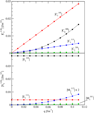
Figure 7: The dependence on the three-momentum transfer $q$ of some electromagnetic RMEs (solid circles); the calculations are at incident proton energy of 0.9 MeV and use the N3LO500/N2LO500 chiral interactions. The solid (dashed) lines show fits of the calculated values using linear (quadratic) parametrizations.

One would naively have expected $|C_{0}^{000}|>|C_{1}^{101}|,|E_{1}^{101}|$, since the energies involved are closer to the $0^{+}$ than to the $1^{-}$ resonance. However, the further suppression with $q$ ($q^{2}$) of $C^{000}_{0}$ relative to $C_{1}^{101}$ ($E_{1}^{101}$) is responsible for inverting the expected trend. As a matter of fact, the $1^{-}$ scattering state plays a very important role in the ${{}^{3}{\rm H}}(p,e^{-}e^{+}){{}^{4}{\rm He}}$ and ${{}^{3}{\rm He}}(n,e^{-}e^{+}){{}^{4}{\rm He}}$ processes.

Figure 8 shows the behavior of selected RMEs as function of the incident proton energy. At the lower end ($\lesssim 0.4$ MeV), the $0^{+}$ resonance is very prominent, but quickly fades away with increasing energy (see $C^{000}_{0}$); by contrast, as the energy increases (exceeding the $n+{{}^{3}{\rm He}}$ threshold) the $1^{-}$ resonance becomes progressively more and more dominant (see $E_{1}^{101}$). The RMEs $E^{111}_{1}$ and $M^{112}_{2}$ increase monotonically with increasing energy, peaking at around about 3.5 MeV.

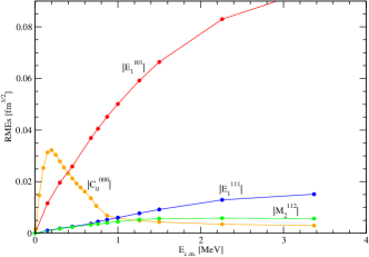
Figure 8: The dependence on the proton incident energy of some RMEs (solid circles); the calculations are at a fixed three-momentum transfer of 0.1 fm^-1 and use the N3LO500/N2LO500 chiral interactions. The lines are to guide the eyes only.

Table 4: RMEs in absolute value (in fm^3/2) corresponding to channels with $J\leq 2$ in the ³H$+p$ scattering wave function, obtained with either the N3LO500/N2LO500 or NVIa/3NIa chiral interactions and accompanying electromagnetic charge and current operators at N4LO. The incident proton energy is 0.9 MeV and the three-momentum transfer $q$ is 0.1 fm^-1.

RMEs$\times 10^{3}$	$p+{{}^{3}{\rm H}}$ wave	N3LO500/N2LO500	NVIa/3NIa
$|C_{0}^{000}|$	${}^{1}S_{0}$	$13.74$	$15.93$
$|M_{1}^{011}|$	${}^{3}S_{1}$	$\phantom{0}0.66$	$\phantom{0}0.14$
$|M_{1}^{211}|$	${}^{3}D_{1}$	$\phantom{0}0.02$	$\phantom{0}0.03$
$|C_{1}^{101}|$	${}^{1}P_{1}$	$26.01$	$25.36$
$|C_{1}^{111}|$	${}^{3}P_{1}$	$\phantom{0}5.14$	$\phantom{0}4.53$
$|E_{1}^{101}|$	${}^{1}P_{1}$	$37.89$	$37.47$
$|E_{1}^{111}|$	${}^{3}P_{1}$	$\phantom{0}3.90$	$\phantom{0}3.27$
$|C_{2}^{202}|$	${}^{1}D_{2}$	$\phantom{0}0.54$	$\phantom{0}0.82$
$|C_{2}^{212}|$	${}^{3}D_{2}$	$\phantom{0}0.01$	$\phantom{0}0.01$
$|E_{2}^{202}|$	${}^{1}D_{2}$	$\phantom{0}0.89$	$\phantom{0}0.73$
$|E_{2}^{212}|$	${}^{3}D_{2}$	$\phantom{0}0.04$	$\phantom{0}0.04$
$|M_{2}^{112}|$	${}^{3}P_{2}$	$\phantom{0}3.38$	$\phantom{0}3.64$
$|M_{2}^{312}|$	${}^{3}F_{2}$	$\phantom{0}0.00$	$\phantom{0}0.00$

Finally, in Table 4 we report the RMEs obtained with the chiral interactions N3LO500/N2LO500 and NVIa/3NIa, and calculated in all cases using the largest number of HH states for full convergence. The model dependence is weak for the largest RMEs. In particular, in the $C_{0}^{000}$ RME we do not observe any critical dependence on the input Hamiltonian. This is in contrast to what happens in the case of the corresponding phase-shift Viviani et al. (2020), which is in fact very sensitive to the Hamiltonian model.

III.5 Results for the electromagnetic cross sections

Here we report cross-section results obtained for the internal pair conversion processes. The calculations use fully converged bound- and scattering-state wave functions (with the largest allowed number of HH states) and the complete N4LO set of electromagnetic charge and current operators.

In Fig. 9 we show the ${{}^{3}{\rm H}}(p,e^{-}e^{+}){{}^{4}{\rm He}}$ four-fold differential cross sections corresponding to the kinematical configuration in which the lepton pair is emitted in the plane perpendicular to the incident proton momentum ($\theta\,$=$\,\theta^{\prime}\,$=$\,90^{\circ}$) and as function of the relative angle $\theta_{ee}$, that is, the angle between the electron and positron momentum. The model dependence is weak, and the curves obtained with the N3LO500/N2LO500 and NVIa/3NIa chiral interactions (and corresponding set of electromagnetic transition operators) essentially overlap, a result we could have anticipated on the basis of the RMEs listed in Table 4.

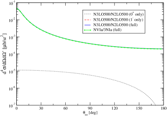
Figure 9: The four-fold differential cross section for the process ${{}^{3}{\rm H}}(p,e^{-}e^{+}){{}^{4}{\rm He}}$ calculated at an incident proton energy of 0.9 MeV; the kinematical configuration corresponds to the lepton pair being emitted in the plane perpendicular to the proton incident momentum, and $\theta_{ee}$ is the angle between the electron and positron momenta. Results obtained with the N3LO500/N2LO500 and NVIa/3NIa Hamiltonians and under different approximations are shown. The dashed red, dot-dash blue, and solid green curves are superimposed and cannot be distinguished. See text for further explanations.

In Fig. 9 we also show the differential cross sections corresponding to the individual ${}^{1}S_{0}$ and ${}^{1}P_{1}$ transitions (again obtained with the N3LO500/N2LO500 model Hamiltonian). In terms of the response functions defined in Eq. (III.1), we observe that for the ${}^{1}S_{0}$ transition only $R_{1}$ is non-vanishing,

$$R_{1}(^{1}S_{0};q)=16\pi^{2}\,|C_{0}^{000}(q)|^{2}\ .$$ (49)

In this respect, it is interesting to note that in the cross section the response function $R_{1}$ is multiplied by $v_{1}$, see Eq. (III.1). In the limit $q\rightarrow 0$ (corresponding to the configuration in which the electrons are emitted back-to-back with the same energy), it is easily seen that this kinematical factor is proportional to $1/q^{2}$; however, this singularity poses no problem, since $|C_{0}^{000}(q)|^{2}\propto q^{4}$. For the ${}^{1}P_{1}$ transitions, the response functions are

$$R_{1}(^{1}P_{1};q) = 48\pi^{2}\cos^{2}\theta_{q}\,|C_{1}^{101}(q)|^{2}\ ,$$

$$R_{2}(^{1}P_{1};q) = 24\pi^{2}\sin(2\theta_{q}){\rm Re}\,\bigl{[}C_{1}^{101*}(q)\,E_{1}^{101}(q)\bigr{]}\ ,$$

$$R_{3}(^{1}P_{1};q) = 0\ ,$$

$$R_{4}(^{1}P_{1};q) = 24\pi^{2}\sin^{2}\theta_{q}\,|E_{1}^{101}(q)|^{2}\ ,$$ (50)

$$R_{5}(^{1}P_{1};q) = -12\pi^{2}\sin^{2}\theta_{q}|E_{1}^{101}(q)|^{2}\ ,$$

$$R_{6}(^{1}P_{1};q) = 0\ ,$$

where $\theta_{q}$ is the polar angle of the three-momentum transfer ${\bm{q}}={\bm{k}}+{\bm{k}}^{\prime}$ in the lab frame. For the kinematical configuration in Fig. 9, we have $\theta_{q}\,$=$\,90^{\circ}$ and hence only $R_{4}$ and $R_{5}$ contribute.

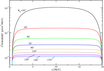
Figure 10: The five-fold differential cross section for the process ${{}^{3}{\rm H}}(p,e^{-}e^{+}){{}^{4}{\rm He}}$ calculated with the N3LO500/N2LO500 Hamiltonian at an incident proton energy of 0.9 MeV as function of the electron energy and for selected angles $\theta_{ee}$; the kinematical configuration is otherwise the same as in Fig. 9.

In Fig. 10 we show the five-fold differential cross section as function of the electron energy $\epsilon$ with $m_{e}\leq\epsilon\leq\epsilon_{max}$ (approximately 20 MeV) for selected angles $\theta_{ee}$. The lepton-pair kinematics is the same as in Fig. 9. As $\theta_{ee}$ increases, the cross section decreases. Away from the endpoints at $\epsilon\,$=$\,m_{e}$ or $\epsilon_{max}$, it is fairly flat. In the limit $\theta_{ee}\longrightarrow 180^{\circ}$ (leptons emitted back-to-back) the cross section remains essentially constant as a consequence of the $q$-independence of the $E_{1}^{1S1}$ RMEs previously discussed.

Table 5: Total cross sections (in $\mu$b) for the processes ${{}^{3}{\rm He}}(n,e^{-}e^{+}){{}^{4}{\rm He}}$ and ${{}^{3}{\rm He}}(n,\gamma){{}^{4}{\rm He}}$ calculated at a number of incident neutron energies $E_{n}$ (in MeV) with the N3LO500/N2LO500 and NVIa/3NIa Hamiltonians. Note that in the energy conservation relations corresponding to pair production and radiative capture, we have used the experimental rather than calculated binding energies of ³He and ⁴He, so that thresholds are at the observed locations.

	N3LO500/N2LO500		NVIa/3NIa
$E_{n}$	${{}^{3}{\rm He}}(n,e^{-}e^{+}){{}^{4}{\rm He}}$	${{}^{3}{\rm He}}(n,\gamma){{}^{4}{\rm He}}$	${{}^{3}{\rm He}}(n,e^{-}e^{+}){{}^{4}{\rm He}}$	${{}^{3}{\rm He}}(n,\gamma){{}^{4}{\rm He}}$
$0.17$	$0.0431$	$20.2$	$0.0396$	$18.9$
$0.35$	$0.0616$	$29.0$	$0.0588$	$28.3$
$0.70$	$0.0893$	$42.0$	$0.0868$	$41.8$
$1.00$	$0.108\phantom{0}$	$50.8$	$0.106\phantom{0}$	$50.8$
$2.00$	$0.146\phantom{0}$	$67.7$	$0.142\phantom{0}$	$67.1$
$3.50$	$0.160\phantom{0}$	$73.1$	$0.155\phantom{0}$	$72.5$

The cross sections at incident proton energies other than 0.9 MeV display the same qualitative features discussed so far. At lower energies, the contribution of the $C_{0}^{000}$ RME becomes more important, while at higher energies (above the $n+{{}^{3}{\rm He}}$ threshold) the cross section is completely dominated by the $C^{101}_{1}$ and $E^{101}_{1}$ RMEs.

Total cross sections for the ${{}^{3}{\rm He}}(n,e^{-}e^{+}){{}^{4}{\rm He}}$ process, calculated with the N3LO500/N2LO500 and NVIa/3NIa Hamiltonian models, are provided in Table 5 at a number of incident neutron energies. For comparison, total cross sections are also reported for the radiative capture process ${{}^{3}{\rm He}}(n,\gamma){{}^{4}{\rm He}}$. We note that pair production cross sections are suppressed by a factor of approximately $500$ relative to radiative capture cross sections.

IV X17-nucleon interactions

In this section we obtain, within $\chi$EFT, the Lagrangians describing the interactions of the X17 with nucleons. We consider, in turn, the cases in which the hypothetical X17 is either a scalar, pseudoscalar, vector or an axial boson. Conventions and notations are as in Appendix A, where we summarize the $\chi$EFT formulation in the $SU(2)$ framework (with up and down quarks), albeit we only include couplings to scalar, pseudoscalar, and vector source terms. The extension of this framework to $SU(3)$ (with up, down, and strange quarks) as well as the inclusion of an axial source term are briefly outlined below.

IV.1 Scalar or pseudoscalar or vector X17

Assuming conservation of parity, the Lagrangian describing the interactions of a scalar X17 boson with up and down quarks is taken as

$${\cal L}^{S}_{q,X}(x)=\sum_{f=u,d}e\,{\varepsilon_{f}\,m_{f}\over\Lambda}\,\overline{f}(x)f(x)\,X(x)\ ,$$ (51)

where $f(x)$ is the field of the quark of flavour $f$, $X(x)$ is the X17 field, and $\Lambda$ is an unknown high-energy mass scale. Note that we have chosen to rescale the coupling constants by the unit electric charge $e$, and have introduced explicitly the quark masses in order to have renormalization-scale invariant amplitudes. This Lagrangian is more conveniently written in terms of the isodoublet quark fields, defined in Appendix A, as

$${\cal L}^{S}_{q,X}(x)=e\,{m_{q}\over\Lambda_{S}}\,\overline{q}(x)(\varepsilon_{0}+\varepsilon_{z}\tau_{3})\,q(x)\,X(x)\ ,$$ (52)

where we have introduced the coupling constants

$$\varepsilon_{0} = {\Lambda_{S}\over\Lambda}\,{m_{u}\,\epsilon_{u}+m_{d}\,\epsilon_{d}\over 2\,m_{q}}\ ,$$ (53)

$$\varepsilon_{z} = {\Lambda_{S}\over\Lambda}\,{m_{u}\,\epsilon_{u}-m_{d}\,\epsilon_{d}\over 2\,m_{q}}\ ,$$ (54)

and a new scale $\Lambda_{S}$ which we set (arbitrarily) at 1 GeV. We have also defined

$$m_{q}={m_{u}+m_{d}\over 2}\ .$$ (55)

From Eq. (52) we identify the isoscalar and isovector scalar sources $s_{0}(x)$ and $s_{3}(x)$, including quark mass contributions, as

$$s_{0}(x) = m_{q}-e\,{m_{q}\over\Lambda_{S}}\varepsilon_{0}\,X(x)\ ,$$ (56)

$$s_{3}(x) = {m_{u}-m_{d}\over 2}-e\,{m_{q}\over\Lambda_{S}}\varepsilon_{z}\,X(x)\ ,$$ (57)

and $s_{1}(x)\,$=$\,s_{2}(x)\,$=$\,0$.

In the chiral Lagrangians (see Appendix A) these scalar sources enter via $\chi(x)\,$=$\,2B_{c}\,s(x)$, where the LEC $B_{c}$ is the quark condensate and $m_{q}\,B_{c}\,$=$\,m^{2}_{\pi}/2$, with $m_{\pi}$ denoting the pion mass. Retaining only up to quadratic terms in the expansion in powers of the pion field yields the Lagrangian

$${\cal L}^{S}_{h,X}(x) = \overline{N}(x)\left[8\,B_{c}\,c_{1}\,s_{0}(x)+4\,B_{c}\,c_{5}\,s_{3}(x)\,\tau_{3}\right]N(x)$$ (58)

$$-\,B_{c}\,s_{0}(x)\,{\bm{\pi}}^{2}(x)\ .$$

We find it convenient to introduce the coupling constants

$$\eta^{S}_{0}=-\frac{4\,c_{1}\,m_{\pi}^{2}}{\Lambda_{S}}\,\varepsilon_{0}\ ,\qquad\eta^{S}_{z}=-\frac{2\,c_{5}\,m_{\pi}^{2}}{\Lambda_{S}}\,\varepsilon_{z}\ ,$$ (59)

in terms of which the nucleon-X17 interaction Lagrangian reads simply as in Eq. (4).

The case in which the X17 is either a pseudoscalar or vector boson can be treated similarly. In the former case we consider the quark-level Lagrangian

$${\cal L}^{P}_{q,X}(x)=\sum_{f=u,d}e\,{\varepsilon_{f}\,m_{f}\over\Lambda}\,\overline{f}(x)(i\gamma^{5})f(x)\,X(x)\ ,$$ (60)

from which we read off the isoscalar and isovector pseudoscalar sources $p_{0}(x)$ and $p_{3}(x)$ as

$$p_{0}(x) = e\,{m_{q}\over\Lambda_{S}}\varepsilon_{0}\,X(x)\ ,$$ (61)

$$p_{3}(x) = e\,{m_{q}\over\Lambda_{S}}\varepsilon_{z}\,X(x)\ ,$$ (62)

where $\varepsilon_{0}$ and $\varepsilon_{z}$ are the combinations of Eqs. (53)–(54). These pseudoscalar sources enter the chiral Lagrangians via the term $2\,iB_{c}\,p(x)$. Interaction terms come from ${\cal L}^{(2)}_{\pi\pi}(x)$ and ${\cal L}^{(3)}_{\pi N}(x)$, giving rise, respectively, to X17-pion and X17-nucleon couplings. While the latter are nominally suppressed by two orders in the power counting, we retain them nevertheless, since it has been speculated Alves (2021) that the X17 may be “piophobic”. After integrating by parts and using the equation of motion to remove derivatives of the nucleon field, the resulting Lagrangian reads

$${\cal L}_{\pi,X}^{P}(x) = 2f_{\pi}B_{c}\,p_{3}(x)\,\pi_{3}(x)$$ (63)

$$+ 4B_{c}m_{N}\,(d_{18}+2\,d_{19})\,\overline{N}(x)i\,\gamma^{5}\,N(x)\,p_{0}(x)$$

$$+ 4B_{c}m_{N}d_{18}\,\overline{N}(x)i\,\gamma^{5}\tau_{z}\,N(x)\,p_{3}(x)\ .$$

We define the coupling constants

$$\eta^{P}_{0} = {2m_{\pi}^{2}m_{N}(d_{18}+2\,d_{19})\over\Lambda_{S}}\,\varepsilon_{0}\ ,$$ (64)

$$\eta^{P}_{z} = \frac{f_{\pi}\,m_{\pi}^{2}}{\Lambda_{S}}\,\varepsilon_{z}\ ,$$ (65)

from which the pseudoscalar interaction Lagrangian follows as in Eq. (5). Note that we have dropped the (direct) isovector X17-nucleon coupling appearing in the third line of Eq. (63).

In the vector boson case, we have

$${\cal L}^{V}_{q,X}(x)=\sum_{f=u,d}e\,\varepsilon_{f}\,\overline{f}(x)\gamma^{\mu}f(x)\,X_{\mu}(x)\ ,$$ (66)

where $X_{\mu}$ is the X17 vector field, and which can be rewritten as usual as

$${\cal L}_{q,X}^{V}=e\,\overline{q}(x)\big{(}\varepsilon_{0}+\varepsilon_{z}\,\tau_{3}\big{)}\gamma^{\mu}q(x)\,X_{\mu}(x)\ .$$ (67)

The parameters $\varepsilon_{0}$ and $\varepsilon_{z}$ are related to the coupling constants of the X17 to the up and down quarks via

$$\varepsilon_{0}={\epsilon_{u}+\epsilon_{d}\over 2}\ ,\qquad\varepsilon_{z}={\epsilon_{u}-\epsilon_{d}\over 2}\ .$$ (68)

The (non-vanishing) vector sources are then given by

$$v_{\mu}^{s}(x) = 3\,e\,\varepsilon_{0}\,X_{\mu}(x)\ ,$$ (69)

$$v_{\mu,3}(x) = e\,\varepsilon_{z}\,X_{\mu}(x)\ ,$$ (70)

and the ensuing nucleon-X17 interaction Lagrangian (at leading order) follows as

$${\cal L}_{N,X}^{V}(x) = \overline{N}(x)\gamma^{\mu}\,[v_{\mu}^{s}(x)+v_{\mu,3}(x)\tau_{3}]N(x)$$

$$+ \!\!{\kappa_{0}\over 4m_{N}}\overline{N}(x)\bigl{[}\partial_{\mu}v^{s}_{\nu}(x)\!-\!\partial_{\nu}v^{s}_{\mu}(x)\bigr{]}\sigma^{\mu\nu}N(x)$$

$$+ \!\!{\kappa_{z}\over 4m_{N}}\overline{N}(x)\bigl{[}\partial_{\mu}v_{\nu,3}(x)\!-\!\partial_{\nu}v_{\mu,3}(x)\bigr{]}\sigma^{\mu\nu}\tau_{3}N(x)\ ,$$

which can be expressed as in Eq. (I.3) by defining the coupling constants

$$\eta_{0}^{V}=3\,\varepsilon_{0}\ ,\,\,\,\,\,\,\eta_{z}^{V}=\varepsilon_{z}\ .$$ (72)

We note that the case of a “proto-phobic” coupling of the X17 corresponds to $\eta_{0}^{V}\approx-\eta_{z}^{V}$.

IV.2 Axial X17

Because of the isospin singlet axial current anomaly Peskin and Schroeder (1995), isoscalar axial sources are absent in the flavor $SU(2)$ Lagrangian of Appendix A. In order to circumvent this difficulty, we extend the theory to flavor $SU(3)$ Scherer and Schindler (2005) by also including strange quarks,

$${\cal L}^{A}_{q,X}(x)=\sum_{f=u,d,s}e\,\varepsilon_{f}\,\overline{f}(x)\gamma^{\mu}\gamma^{5}\,f(x)\,X_{\mu}(x)\ ,$$ (73)

and define the field $q(x)$ as

$$q(x)=\left[\!\begin{array}[]{c}u(x)\\ d(x)\\ s(x)\end{array}\!\right].$$ (74)

If we ignore strange-quark components in the nucleon,

$$\langle N|\overline{s}(x)\gamma_{\mu}\gamma^{5}s(x)|N\rangle=0\ ,$$ (75)

we can then identify the isoscalar axial-source term with one of the $SU(3)$ axial currents, conserved in the chiral limit where the masses of up, down, and strange quarks vanish, that is,

$$\langle N|\overline{u}(x)\gamma_{\mu}\gamma^{5}u(x)\!+\!\overline{d}(x)\gamma_{\mu}\gamma^{5}d(x)|N\rangle\!\longrightarrow\!\langle N|a_{\mu,8}(x)|N\rangle\ ,$$ (76)

where the current $a_{\mu,8}(x)$ is

$$a_{\mu,8}(x)\! = \!\overline{u}(x)\gamma_{\mu}\gamma^{5}u(x)\!+\overline{d}(x)\gamma_{\mu}\gamma^{5}d(x)\!-2\,\overline{s}(x)\gamma_{\mu}\gamma^{5}s(x)$$ (77)

$$= \sqrt{3}\,\overline{q}(x)\gamma_{\mu}\gamma^{5}\lambda_{8}\,q(x)\ ,$$

and $\lambda_{8}$ is the Gell-Mann matrix

$$\lambda_{8}=\frac{1}{\sqrt{3}}\begin{pmatrix}1&0&0\\ 0&1&0\\ 0&0&-2\end{pmatrix}\ .$$ (78)

The relevant piece of the flavor $SU(3)$ quark-level Lagrangian reads Scherer and Schindler (2005)

$${\cal L}_{q,X}^{A}=\overline{q}(x)\,a_{\mu}(x)\gamma^{\mu}\gamma^{5}\,q(x)\,\ ,$$ (79)

where

$$a_{\mu}(x)=a_{\mu,3}(x)\,\lambda_{3}+a_{\mu,8}(x)\,\lambda_{8}\ ,$$ (80)

and

$$a_{\mu,3}(x)=e\,\varepsilon_{z}\,X_{\mu}(x)\ ,\qquad a_{\mu,8}(x)=\sqrt{3}\,e\,\varepsilon_{0}X_{\mu}(x)\ ,$$ (81)

with $\varepsilon_{0}$ and $\varepsilon_{z}$ defined as in Eq. (68). The Gell-Mann matrix $\lambda_{3}$ is the $SU(3)$ extension of the Pauli matrix $\tau_{3}$, namely

$$\lambda_{3}=\begin{pmatrix}1&0&0\\ 0&-1&0\\ 0&0&0\end{pmatrix}.$$ (82)

At the hadronic level, the flavor $SU(3)$ chiral Lagrangian is written in terms of the baryon-field matrix

$$B=\begin{pmatrix}\Sigma^{0}/\sqrt{2}+\Lambda/\sqrt{6}&\Sigma^{+}&p\\ \Sigma^{-}&-\Sigma^{0}/\sqrt{2}+\Lambda/\sqrt{6}&n\\ \Xi^{-}&\Xi^{0}&-2\,\Lambda/\sqrt{6}\end{pmatrix}\ ,$$ (83)

and meson-field matrix

$$\Phi=\begin{pmatrix}\pi_{3}+\eta/\sqrt{3}&\pi_{1}+i\,\pi_{2}&\sqrt{2}\,K^{+}\\ \pi_{1}-i\,\pi_{2}&-\pi_{3}+\eta/\sqrt{3}&\sqrt{2}\,K^{0}\\ \sqrt{2}\,K^{-}&\sqrt{2}\,\overline{K}^{\,0}&-2\,\eta/\sqrt{3}\end{pmatrix}\ ,$$ (84)

where $\Sigma^{\pm}$, $K^{\pm}$, etc., are the fields associated with the various strange baryons and mesons. The building blocks are $3\times 3$ matrices, defined as

$$U = 1+{i\over f_{\pi}}\Phi-{1\over 2\,f_{\pi}^{2}}\,\Phi^{2}+\cdots\ ,$$ (85)

$$D_{\mu}B = \partial_{\mu}B+[\Gamma_{\mu}\,,\,B]\ ,$$ (86)

with the remaining auxiliary fields $u$, $u_{\mu}$, $\Gamma_{\mu}$, and $F_{\mu\nu}^{\pm}$ as given in Eq. (A). Here, we specialize to the case of an external axial current only, and therefore set $r_{\mu}(x)\,$=$\,-\ell_{\mu}(x)\,$=$\,a_{\mu}(x)$, with $a_{\mu}(x)$ as in Eq. (80). In this extended framework, the meson-baryon Lagrangian at leading order reads Scherer and Schindler (2005)

$$\mathcal{L}_{mB}^{(1)} = \langle\,\overline{B}(i\,\gamma_{\mu}D^{\mu}-M_{B})B+{D\over 2}\overline{B}\gamma^{\mu}\gamma^{5}\{u_{\mu}\,,\,B\}$$ (87)

$$+{F\over 2}\bar{B}\gamma^{\mu}\gamma^{5}[u_{\mu}\,,\,B]\,\rangle\ ,$$

where $\langle\cdots\rangle$ indicates a trace in flavor space, $M_{B}$ is the mass matrix of the baryon octet, and $D$ and $F$ are LECs. Expanding in powers of the meson fields $\Phi$ and considering only pion-nucleon-X17 interaction terms, we obtain

$$\mathcal{L}^{A}_{N,X}(x) = (D+F)\,\overline{N}(x)\gamma^{\mu}\gamma^{5}\tau_{3}\,N(x)\,a_{\mu,3}(x)$$ (88)

$$+\frac{3\,F-D}{\sqrt{3}}\overline{N}(x)\,\gamma^{\mu}\gamma^{5}N(x)\,a_{\mu,8}(x)\ ,$$

which can be cast in the form of Eq. (7) by defining the coupling constants

$$\eta_{0}^{A}=(3\,F-D)\,\varepsilon_{0}\ ,\qquad\eta_{z}^{A}=(F+D)\,\varepsilon_{z}\ .$$ (89)

We note in closing that the term $\langle\nabla_{\mu}U^{\dagger}\nabla^{\mu}U\rangle$ in the meson-meson Lagrangian at leading order also generates an interaction term involving the direct coupling of the pion to the axial field of the form $\partial^{\mu}\pi_{3}(x)\,X_{\mu}(x)$. As mentioned in Sec. I.3, we ignore it here for simplicity.

V X17-induced nuclear currents

The pair production amplitude on a single nucleon $T_{fi}^{cX}(N)$ induced by each of the (leading order) Lagrangians in Eqs. (4)–(7) can be easily calculated, for example, in time-ordered perturbation theory. The general structure is as given in Eq. (9) with $j_{fi}^{cX}$ replaced by the single-nucleon current $j^{cX}_{fi}(N)$, that is,

$$T_{fi}^{cX}(N)=4\pi\alpha\,\frac{\varepsilon_{e}\,\overline{u}({{\bm{k}}s})\,\Gamma_{c}\,v({{\bm{k}}^{\prime}s^{\prime}})\,j_{fi}^{cX}(N)}{q^{\mu}\,q_{\mu}-M_{X}^{2}}\ ,$$ (90)

where

$$j_{fi}^{SX}(N) = \overline{u}({{\bm{p}}^{\prime}s_{N}^{\prime}})\,u({{\bm{p}}s_{N}})\,\chi^{\dagger}_{t_{N}^{\prime}}P^{SX}\chi_{t_{N}}\ ,$$ (91)

$$j_{fi}^{PX}(N) = \frac{\overline{u}({{\bm{p}}^{\prime}s_{N}^{\prime}})\gamma^{\mu}\gamma_{5}\,i\,q_{\mu}\,u({{\bm{p}}s_{N}})}{q^{\mu}q_{\mu}-m_{\pi}^{2}}\,\chi^{\dagger}_{t_{N}^{\prime}}P^{PX}\chi_{t_{N}}$$ (92)

$$+ \overline{u}({{\bm{p}}^{\prime}s_{N}^{\prime}})\,i\gamma^{5}\,u({{\bm{p}}s_{N}})\,\chi^{\dagger}_{t_{N}^{\prime}}\overline{P}^{PX}\chi_{t_{N}}\ ,$$

$$j_{fi}^{VX}(N) = -\overline{u}({{\bm{p}}^{\prime}s_{N}^{\prime}})\,\gamma^{\mu}\,u({{\bm{p}}s_{N}})\,\chi^{\dagger}_{t_{N}^{\prime}}P^{VX}\chi_{t_{N}}$$

$$+\frac{i}{2\,m_{N}}\,\overline{u}({{\bm{p}}^{\prime}s_{N}^{\prime}})\,\sigma^{\mu\nu}q_{\nu}\,u({{\bm{p}}s_{N}})\,\chi^{\dagger}_{t_{N}^{\prime}}\overline{P}^{VX}\chi_{t_{N}}\ ,$$

$$j_{fi}^{AX}(N) = -\overline{u}({{\bm{p}}^{\prime}s_{N}^{\prime}})\,\gamma^{\mu}\,\gamma_{5}\,u({{\bm{p}}s_{N}})\,\chi^{\dagger}_{t_{N}^{\prime}}P^{AX}\chi_{t_{N}}\ ,$$ (94)

and $\chi_{t_{N}}$ and $\chi_{t^{\prime}_{N}}$ denote the initial and final nucleon isospin states, respectively. We have defined the isospin operators

$$P^{SX}=\eta_{0}^{S}+\eta_{z}^{S}\,\tau_{3}\ ,$$ (95)

and similarly for $P^{VX}$ and $P^{AX}$ with the $\eta^{S}_{0}$ and $\eta_{z}^{S}$ replaced by the corresponding set of coupling constants, and

$$P^{PX} = \frac{g_{A}}{2\,f_{\pi}}\,\eta^{P}_{z}\,\tau_{3}\ ,$$ (96)

$$\overline{P}^{PX} = \eta^{P}_{0}\ ,$$ (97)

$$\overline{P}^{VX} = \kappa_{0}\,\eta_{0}^{V}+\kappa_{z}\,\eta_{z}^{V}\,\tau_{3}\ .$$ (98)

The nuclear currents follow by retaining the leading-order term in the non-relativistic expansion of $j^{cX}(N)$ and by summing over the individual nucleons (impulse approximation). We define matrix elements of these currents between the initial 3+1 scattering state and final ⁴He ground state as in Eq. (27)

$$j^{cX}_{fi}=\langle\Psi({\bm{p}}-{\bm{q}})|j^{cX\,\dagger}({\bm{q}})|\Psi^{(\gamma)}_{m_{3},m_{1}}({\bm{p}})\rangle\ ,$$ (99)

where the $j^{cX}({\bm{q}})$ are single-nucleon operators which in configuration-space can be written in terms of the following operator structures, stripped of the coupling constants $\eta^{c}_{0,z}$,

$$\rho^{S\lambda}({\bm{q}}) = \sum_{i=1}^{A}e^{i{\bm{q}}\cdot{\bm{r}}_{i}}\,P^{\lambda}_{i}\ ,$$ (100)

$$\rho^{P\lambda}({\bm{q}}) = \sum_{i=1}^{A}e^{i{\bm{q}}\cdot{\bm{r}}_{i}}\,i\,\hat{\bm{q}}\cdot{\bm{\sigma}}_{i}\,P^{\lambda}_{i}\ ,$$ (101)

$$\rho^{A\lambda}({\bm{q}}) = \sum_{i=1}^{A}\frac{1}{2\,m_{N}}\,\left[e^{i{\bm{q}}\cdot{\bm{r}}_{i}}\,,\,{\bm{p}}_{i}\cdot{\bm{\sigma}}_{i}\right]_{+}\,P^{\lambda}_{i}\ ,$$ (102)

$${\bm{j}}^{V\lambda}({\bm{q}}) = \sum_{i=1}^{A}\frac{1}{2\,m_{N}}\left[e^{i{\bm{q}}\cdot{\bm{r}}_{i}}\,,\,{\bm{p}}_{i}\right]_{+}P^{\lambda}_{i}\ ,$$ (103)

$$\overline{{\bm{j}}}^{V\lambda}({\bm{q}}) = \sum_{i=1}^{A}\frac{i}{2\,m_{N}}\,e^{i{\bm{q}}\cdot{\bm{r}}_{i}}\,{\bm{q}}\times{\bm{\sigma}}_{i}\,P^{\lambda}_{i}\ ,$$ (104)

$${\bm{j}}^{A\lambda}({\bm{q}}) = \sum_{i=1}^{A}e^{i{\bm{q}}\cdot{\bm{r}}_{i}}\,{\bm{\sigma}}_{i}\,P^{\lambda}_{i}\ ,$$ (105)

where $\lambda=\pm$ with $P^{+}_{i}\,$=$\,1$ and $P^{-}_{i}\,$=$\,\tau_{i,3}$, ${\bm{p}}_{i}$ is the momentum operator, and $[\cdots]_{+}$ denotes the anticommutator. Note that the operators are defined to be adimensional.

In the calculation we have retained the space and time components of, respectively, the vector and axial currents, even though they are suppressed in the power counting relative to the corresponding time and space components. As a matter of fact, these terms give important contributions by connecting the 3+1 ${}^{1}P_{1}$ and ${}^{3}P_{0}$ continuum states to the ⁴He ground state via $E_{1}(V)$ and $C_{0}(A)$ multipole transitions.

VI X17-induced cross sections

In this section we compute the cross section including the contribution of the X17 boson. This cross section consists of a purely electromagnetic term, which we have already analyzed in Sec. III, an interference term between the virtual photon and X17 amplitudes,

$$d\sigma_{X}={1\over 4}\sum_{m_{3}m_{1}}\sum_{ss^{\prime}}\frac{T^{*}_{fi}T^{cX}_{fi}+{\rm c.c.}}{v_{r}}\,d\phi\ ,$$ (106)

and a term associated with the X17 exchange,

$$d\sigma_{XX}={1\over 4}\sum_{m_{3}m_{1}}\sum_{ss^{\prime}}\frac{|T^{cX}_{fi}|^{2}}{v_{r}}\,d\phi\ ,$$ (107)

where $T_{fi}$ and $T^{cX}_{fi}$ are the amplitudes given in Eqs. (1) and (9), the phase-space factor $d\phi$ has been defined in Eq. (30), and the superscript $\gamma$ identifying the initial 3+1 nuclear state ($p$+³H or $n$+³He) is understood. Standard trace theorems are used to evaluate the lepton tensors entering these cross sections. Noting that $\Gamma^{c\,\dagger}=\gamma^{0}\,\Gamma^{c}\,\gamma^{0}$, we find

• for the scalar case:

  $$\sum_{ss^{\prime}}\ell^{\mu}_{{\bm{k}}s,{\bm{k}}^{\prime}s^{\prime}}\,\ell^{S\,*}_{{\bm{k}}s,{\bm{k}}^{\prime}s^{\prime}} = {m_{e}\over\epsilon\epsilon^{\prime}}\,(k^{\prime\mu}-k^{\mu})\ ,$$ (108)

  $$\sum_{ss^{\prime}}\ell^{S}_{{\bm{k}}s,{\bm{k}}^{\prime}s^{\prime}}\ell^{S\,*}_{{\bm{k}}s,{\bm{k}}^{\prime}s^{\prime}} = {1\over\epsilon\epsilon^{\prime}}\,(k\cdot k^{\prime}-m_{e}^{2})\ ;$$ (109)

• for the pseudoscalar case, the mixed trace and hence the interference term in the cross section vanish, while

  $$\sum_{ss^{\prime}}\ell^{P}_{{\bm{k}}s,{\bm{k}}^{\prime}s^{\prime}}\ell^{P\,*}_{{\bm{k}}s,{\bm{k}}^{\prime}s^{\prime}}={1\over\epsilon\epsilon^{\prime}}\,(k\cdot k^{\prime}+m_{e}^{2})\ ;$$ (110)

• for the vector case, the mixed and direct traces are of course the same, and

  $$\sum_{ss^{\prime}}\ell^{\mu}_{{\bm{k}}s,{\bm{k}}^{\prime}s^{\prime}}\,\ell^{\nu\,*}_{{\bm{k}}s,{\bm{k}}^{\prime}s^{\prime}} = {1\over\epsilon\epsilon^{\prime}}[k^{\mu}k^{\prime\nu}+k^{\prime\mu}k^{\nu}$$ (111)

  $$\,-\,g^{\mu\nu}(k\cdot k^{\prime}+m_{e}^{2})]\ ;$$

• for the axial case:

  $$\sum_{ss^{\prime}}\ell^{\mu}_{{\bm{k}}s,{\bm{k}}^{\prime}s^{\prime}}\,\ell^{\nu A\,*}_{{\bm{k}}s,{\bm{k}}^{\prime}s^{\prime}} = {i\over\epsilon\epsilon^{\prime}}\,\epsilon^{\mu\nu\alpha\beta}k_{\alpha}k^{\prime}_{\beta}\ ,$$ (112)

  $$\sum_{ss^{\prime}}\ell^{\mu A}_{{\bm{k}}s,{\bm{k}}^{\prime}s^{\prime}}\ell^{\nu A\,*}_{{\bm{k}}s,{\bm{k}}^{\prime}s^{\prime}} = {1\over\epsilon\epsilon^{\prime}}[k^{\mu}k^{\prime\nu}+k^{\prime\mu}k^{\nu}$$ (113)

  $$\,-\,g^{\mu\nu}(k\cdot k^{\prime}-m_{e}^{2})]\ .$$

Table 6: The reduced response functions $R^{X}_{n,\lambda}$ with $\lambda\,$=$\pm$ entering the interference cross section $\sigma_{X}$ and the kinematical factors $v^{X}_{n}$. The matrix elements $\rho_{fi}$ and $j^{\pm}_{fi}$ of the time and space components of the electromagnetic current are defined as in Eq. (37). The matrix elements $\rho^{X}_{fi}$ and $j^{X,\pm}_{fi,\lambda}$ are defined similarly with the X17-induced current replacing the electromagnetic one; of course, since the X17 current is not assumed to be conserved, a longitudinal matrix element $j^{X,z}_{fi,\lambda}$ is also present (see text). Note that there is no contribution to the inference cross section in the case of a pseudoscalar X17. We have defined $u\,$=$\,\omega/q$ and the spherical components $P_{\pm}\,$=$\,\mp(P_{x}\pm i\,P_{y})/\sqrt{2}$ with ${\bm{P}}\,$=${\bm{k}}-{\bm{k}}^{\prime}$. Moreover, $P_{z}=\hat{\bm{e}}_{z}\cdot{\bm{P}}$. Lastly, the second column specifies the character—purely longitudinal (L), purely transverse (T), or longitudinal-transverse (LT)—of the given $R^{X}_{n,\lambda}$.

$n$	Character	$R_{n,\lambda}^{X}$	$v_{n}^{X}$
			$S$	$V$	$A$
$1$	L	$\sum_{m_{3}m_{1}}\rho_{fi}^{*}\,\,\rho^{X}_{fi,\lambda}$	$m_{e}\,(P_{0}-uP_{z})$	$(P_{0}-uP_{z})P_{0}/2+(m_{e}^{2}+k\cdot k^{\prime})$
$2$	L	$\sum_{m_{3}m_{1}}\rho_{fi}^{*}\,\,j^{X,z}_{fi,\lambda}$		$-(P_{0}-uP_{z})P_{z}/2-u(m_{e}^{2}+k\cdot k^{\prime})$
$3$	LT	$\sum_{m_{3}m_{1}}\rho^{*}_{fi}\,\,j^{X,+}_{fi,\lambda}$		$(P_{0}-uP_{z})P_{-}/2$	$-Q^{2}P_{-}/(2\,q)$
$4$	LT	$\sum_{m_{3}m_{1}}\rho^{*}_{fi}\,\,j^{X,-}_{fi,\lambda}$		$(P_{0}-uP_{z})P_{+}/2$	$Q^{2}P_{+}/(2\,q)$
$5$	LT	$\sum_{m_{3}m_{1}}j^{+\,*}_{fi}\,\,\rho^{X}_{fi,\lambda}$	$-m_{e}\,P_{+}$	$-P_{0}P_{+}/2$	$-qP_{+}/2$
$6$	LT	$\sum_{m_{3}m_{1}}j^{-\,*}_{fi}\,\,\rho^{X}_{fi,\lambda}$	$-m_{e}\,P_{-}$	$-P_{0}P_{-}/2$	$qP_{-}/2$
$7$	LT	$\sum_{m_{3}m_{1}}j^{+\,*}_{fi}\,\,j^{X,z}_{fi,\lambda}$		$P_{z}P_{+}/2$	$\omega P_{+}/2$
$8$	LT	$\sum_{m_{3}m_{1}}j^{-\,*}_{fi}\,\,j^{X,z}_{fi,\lambda}$		$P_{z}P_{-}/2$	$-\omega P_{-}/2$
$9$	T	$\sum_{m_{3}m_{1}}\bigl{(}j^{+\,*}_{fi}\,j^{X,+}_{fi,\lambda}+j^{-\,*}_{fi}\,j^{X,-}_{fi,\lambda}\bigr{)}$		$(P_{x}^{2}+P_{y}^{2})/4-k\cdot k^{\prime}-m_{e}^{2}$
$10$	T	$\sum_{m_{3}m_{1}}\bigl{(}j^{+\,*}_{fi}\,j^{X,+}_{fi,\lambda}-j^{-\,*}_{fi}\,j^{X,-}_{fi,\lambda}\bigr{)}$			$(P_{0}\,q-P_{z}\,\omega)/2$
$11$	T	$\sum_{m_{3}m_{1}}j^{+\,*}_{fi}\,\,j^{X,-}_{fi,\lambda}$		$-P_{+}^{2}/2$
$12$	T	$\sum_{m_{3}m_{1}}j^{-\,*}_{fi}\,\,j^{X,+}_{fi,\lambda}$		$-P_{-}^{2}/2$

In analogy to the purely electromagnetic case in Eq. (38), we express the interference and direct five-fold differential cross sections as

$$\sigma_{X}(\epsilon,\hat{{\bm{k}}},\hat{{\bm{k}}}^{\prime})\!=\!\frac{\alpha^{2}}{(2\pi)^{3}}{k\,k^{\prime}\over Q^{2}}\frac{f_{\rm rec}}{v_{r}}\,\varepsilon_{e}\bigg{[}\frac{R^{X}_{fi}}{Q^{2}-M_{X}^{2}}+{\rm c.c.}\bigg{]}\ ,$$ (114)

$$\sigma_{XX}(\epsilon,\hat{{\bm{k}}},\hat{{\bm{k}}}^{\prime})\!=\!\frac{\alpha^{2}}{(2\pi)^{3}}{k\,k^{\prime}\over|Q^{2}-M_{X}^{2}|^{2}}\frac{f_{\rm rec}}{v_{r}}\,\varepsilon_{e}^{2}\,R^{XX}_{fi}\ ,$$ (115)

where $\varepsilon_{e}$ is the coupling constant of the electron to the X17 particle, and $R^{X}_{fi}$ and $R^{XX}_{fi}$ denote the nuclear responses associated with, respectively, the interference and direct terms (the former one is generally complex). Note that, when accounting for the X17 width, we make the replacement of Eq. (10) in the X17 propagator, yielding a complex function of the mass $M_{X}$ and width $\Gamma_{X}$. Of course, the full cross section results from Eq. (14).

The interference and direct nuclear responses can be conveniently cast into the forms

$$R_{fi}^{X}\! = \!\sum_{n=1}^{12}v_{n}^{X}\left(\eta_{0}\,R^{X}_{n,+}+\eta_{z}R_{n,-}^{X}\right)\ ,$$ (116)

$$R_{fi}^{XX}\!\! = \!\!\sum_{n=1}^{10}v_{n}^{XX}\left(\eta^{2}_{0}\,R^{XX}_{n,++}+2\,\eta_{0}\,\eta_{z}R_{n,+-}^{XX}+\eta^{2}_{z}\,R^{XX}_{n,--}\right)\ ,$$

where the $v_{n}^{X}$ and $v_{n}^{XX}$ involve the lepton kinematic variables and the reduced response functions $R^{X}_{n,\lambda}$ and $R^{XX}_{n,\lambda\lambda^{\prime}}$ denote appropriate combinations of the matrix elements of the electromagnetic and X17-induced currents, as indicated in Tables 6 and 7 for the various possibilities ($S$, $P$, $V$, and $A$). The dependence of the reduced response functions on the coupling constants $\varepsilon_{0}$ and $\varepsilon_{z}$ of the X17 to the quarks can be obtained using Eqs. (59), (64), (65), (72), and (89). The index $\lambda=\pm$ specifies the matrix elements calculated using either the isoscalar ($+$) and isovector ($-$) component of the various operators.

Table 7: The reduced response functions $R^{XX}_{n,\lambda\lambda^{\prime}}$ with $\lambda,\lambda^{\prime}\,$=$\pm$ entering the direct cross section $\sigma_{XX}$ and the kinematical factors $v^{XX}_{n}$; remaining notation as in Table 6. The upper and lower signs in the $v_{n}^{XX}$ correspond to the $S/V$ or $P/A$ cases, respectively.

$n$	Character	$R^{XX}_{n,\lambda\lambda^{\prime}}$	$v_{n}^{XX}$
			$S,P$	$V,A$
$1$	L	$\sum_{m_{3}m_{1}}{\rm Re}\,\big{(}\rho^{X*}_{fi,\lambda}\,\,\rho^{X}_{fi,\lambda^{\prime}}\big{)}$	$k\cdot k^{\prime}\mp m_{e}^{2}$	$2\epsilon\epsilon^{\prime}-k\cdot k^{\prime}\mp m_{e}^{2}$
$2$	L	$\sum_{m_{3}m_{1}}{\rm Re}\,\bigl{(}\rho^{X*}_{fi,\lambda}\,\,j^{X,z}_{fi,\lambda^{\prime}}+\rho^{X*}_{fi,\lambda^{\prime}}\,\,j^{X,z}_{fi,\lambda}\bigr{)}/2$		$-\omega q+P_{0}P_{z}$
$3$	L	$\sum_{m_{3}m_{1}}{\rm Re}\,\bigl{(}j^{X,z\,*}_{fi,\lambda}\,\,j^{X,z}_{fi,\lambda^{\prime}}\bigr{)}$		$(q^{2}-P_{z}^{2})/2+k\cdot k^{\prime}\pm m_{e}^{2}$
$4$	LT	$\sum_{m_{3}m_{1}}{\rm Re}\,\bigl{[}\rho^{X\,*}_{fi,\lambda}\,\bigl{(}j^{X,+}_{fi,\lambda^{\prime}}-j^{X,-}_{fi,\lambda^{\prime}}\bigr{)}+\rho^{X\,*}_{fi,\lambda^{\prime}}\bigl{(}j^{X,+}_{fi,\lambda}-j^{X,-}_{fi,\lambda}\bigr{)}\bigr{]}/2$		$-P_{0}P_{x}/\sqrt{2}$
$5$	LT	$\sum_{m_{3}m_{1}}{\rm Im}\,\bigl{[}\rho^{X\,*}_{fi,\lambda}\,\bigl{(}j^{X,+}_{fi,\lambda^{\prime}}+j^{X,-}_{fi,\lambda^{\prime}}\bigr{)}+\rho^{X\,*}_{fi,\lambda^{\prime}}\bigl{(}j^{X,+}_{fi,\lambda}+j^{X,-}_{fi,\lambda}\bigr{)}\bigr{]}/2$		$-P_{0}P_{y}/\sqrt{2}$
$6$	LT	$\sum_{m_{3}m_{1}}{\rm Re}\,\bigl{[}j^{X,z\,*}_{fi,\lambda}\,\bigl{(}j^{X,+}_{fi,\lambda^{\prime}}-j^{X,-}_{fi,\lambda^{\prime}}\bigr{)}+j^{X,z\,*}_{fi,\lambda^{\prime}}\bigl{(}j^{X,+}_{fi,\lambda}-j^{X,-}_{fi,\lambda}\bigr{)}\bigr{]}/2$		$P_{z}P_{x}/\sqrt{2}$
$7$	LT	$\sum_{m_{3}m_{1}}{\rm Im}\,\bigl{[}j^{X,z\,*}_{fi,\lambda}\,\bigl{(}j^{X,+}_{fi,\lambda^{\prime}}+j^{X,-}_{fi,\lambda^{\prime}}\bigr{)}+j^{X,z\,*}_{fi,\lambda^{\prime}}\bigl{(}j^{X,+}_{fi,\lambda}+j^{X,-}_{fi,\lambda}\bigr{)}\bigr{]}/2$		$P_{z}P_{y}/\sqrt{2}$
$8$	T	$\sum_{m_{3}m_{1}}{\rm Re}\,\bigl{(}j^{X,+\,*}_{fi,\lambda}\,\,j^{X,+}_{fi,\lambda^{\prime}}+j^{X,-\,*}_{fi,\lambda}\,\,j^{X,-}_{fi,\lambda^{\prime}}\bigr{)}$		$-(P_{x}^{2}+P_{y}^{2})/4+k\cdot k^{\prime}\pm m_{e}^{2}$
$9$	T	$\sum_{m_{3}m_{1}}{\rm Re}\,\bigl{(}j^{X,+\,*}_{fi,\lambda}\,\,j^{X,-}_{fi,\lambda^{\prime}}+j^{X,+\,*}_{fi,\lambda^{\prime}}\,\,j^{X,-}_{fi,\lambda}\bigr{)}/2$		$(P_{x}^{2}-P_{y}^{2})/2$
$10$	T	$\sum_{m_{3}m_{1}}{\rm Im}\,\bigl{(}j^{X,+\,*}_{fi,\lambda}\,\,j^{X,-}_{fi,\lambda^{\prime}}+j^{X,+\,*}_{fi,\lambda^{\prime}}\,\,j^{X,-}_{fi,\lambda}\bigr{)}/2$		$-P_{x}P_{y}$

Since the vector and axial X17-induced currents are not assumed to be conserved, in the reduced response functions listed in Tables 6 and 7 there is a contribution involving the longitudinal component of the current,

$$j^{X,z}_{fi,\lambda}=\langle\Psi|\hat{\bm{e}}_{z}\cdot{\bm{j}}^{cX\,\dagger}_{\lambda}({\bm{q}})|\Psi^{(\gamma)}\rangle\ ,$$ (117)

which is of course absent in the purely electromagnetic case. The matrix elements of the charge and those of the transverse components of the current are expanded in RMEs of multipole operators as in Eqs. (45)–(46). The longitudinal current matrix element has a similar expansion

$$j^{X,z}_{fi,\lambda}=\sqrt{4\pi}(-{i})^{J}(-)^{J-J_{z}}D_{-J_{z},0}^{J}(-\phi,-\theta,0)\,L_{J}^{LSJ}(q)\ .$$ (118)

Of course, the multipole parities for the $S$ and $V$ currents are opposite to those of the $P$ and $A$ currents.

Lastly, the contribution resulting from the contraction of the $q^{\mu}\,q^{\nu}/M_{X}^{2}$ term in the propagator of the X17 boson with the leptonic tensor vanishes in the vector case and is neglected in the axial case, since it is proportional to $(m_{e}/M_{X})^{2}\approx 0.0009$.

VII Results including the X17 boson

In this section we provide further numerical details in support of the cross section results reported in Sec. I.4. We begin by analyzing the relevant RMEs contributing to the transition mediated by the X17 boson. The RMEs contributing to the purely electromagnetic transition have already been analyzed in Sec. III.4.

VII.1 Numerical results for the RMEs

The relevant operators are given in Eqs. (100)–(105). The RMEs associated with a $S$ or $V$ exchange are those in Table 2 (except that the longitudinal RMEs are not listed; they connect to the same states as the charge RMEs), while the RMEs contributing to a transition mediated by a $P$ or $A$ exchange are listed in Table 8.

Table 8: The RMEs contributing to a transition mediated by a pseudoscalar or axial X17 exchange. Remaining notation as in Table 3.

state	${}^{2S+1}L_{J}$	charge multipoles	current multipoles
$0^{+}$	${}^{1}S_{0}$	$-$	$-$
$0^{-}$	${}^{3}P_{0}$	$C_{0}^{110}$	$L_{0}^{110}$
$1^{+}$	${}^{3}S_{1},{}^{3}D_{1}$	$C_{1}^{LS1}$	$E_{1}^{LS1},L_{1}^{LS1}$
$1^{-}$	${}^{1}P_{1},{}^{3}P_{1}$	$-$	$M_{1}^{1S1}$
$2^{+}$	${}^{1}D_{2},{}^{3}D_{2}$	$-$	$M_{2}^{2S2}$
$2^{-}$	${}^{3}P_{2},{}^{3}F_{2}$	$C_{2}^{LS2}$	$E_{2}^{LS2},L_{2}^{LS2}$

In the following figures we consider separately the isoscalar ($+$) and isovector ($-$) components of the operators as given explicitly in Eqs. (100)–(105). The corresponding RMEs carry a superscript $+$ or $-$. Of course, the isoscalar and isovector terms in the $S$ operator are identical to the corresponding ones in the $V$ charge operator. However, the isovector $P$ operator and isovector term in the $A$ charge operator differ, the former involving $\hat{\bm{q}}\cdot{\bm{\sigma}}_{i}$ and the latter involving ${\bm{p}}_{i}\cdot{\bm{\sigma}}_{i}$.

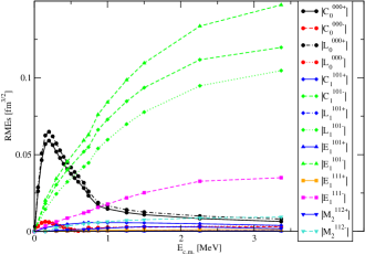
Figure 11: RMEs (in absolute value) resulting from $V$-induced transitions, see text for additional information. The $C_{J}^{LSJ\pm}$ ($L_{J}^{LSJ\pm}$, $E_{J}^{LSJ\pm}$, and $M_{J}^{LSJ\pm}$) RMEs come from matrix elements of the isoscalar ($+$) and isovector ($-$) charge (current) operator. The calculations are for the ³H($p,e^{+}e^{-})^{4}$He process and are based on the N3LO500/N2LO500 interactions.

In Fig. 11, we show the RMEs, as functions of the relative energy, calculated with the $V$ operators. The results are similar to those shown in Fig. 8. However, since we separate the isoscalar and isovector components of the transition operators, we can observe the effect of the different isospin content of the various initial states. For example, in the low-energy regime only the RME associated with the isoscalar component of the $V$ charge operator displays a resonant behavior, confirming the predominant $T\,$= 0 character of the $0^{+}$ resonance. At higher energies, by contrast, the dominant contribution is from the RMEs induced by the isovector $V$ charge and current operators (specifically, the RMEs $C_{1}^{101-}$, $L_{1}^{101-}$, and $E_{1}^{101-}$), attesting to the dominant $T\,$= 1 nature of the $1^{-}$ resonance; indeed, the corresponding isoscalar RMEs are roughly an order of magnitude smaller. This is also related to the fact that, for small $q$, the electric dipole operator is dominated by the isovector component Walecka (1995).

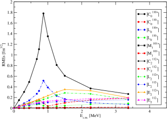
Figure 12: Same as in Fig. 11 bur for $A$-induced transitions.

In Figs. 12 and 13, we show the RMEs, as functions of the relative energy, calculated only with the $A$ and $P$ operators. Note that the charge RMEs are calculated using the operator of Eq. (101) for $P$-exchange and the operator of Eq. (102) for $A$-exchange. These RMEs are qualitatively similar. The resonant behavior of the $C_{0}^{110+}$ RME in both figures, due to the transition from the initial ${}^{3}P_{0}$ state to the final ground state, is evident. This behavior is related to the presence in the ${{}^{4}{\rm He}}$ spectrum of a $0^{-}$ resonance just above the opening of the $n+^{3}$He channel. The very broad peaks in the $C_{2}^{LS2\pm}$ and $E_{2}^{LS2\pm}$ RMEs, connected to the presence of $2^{-}$ resonant states in the ${{}^{4}{\rm He}}$ spectrum, should also be noted.

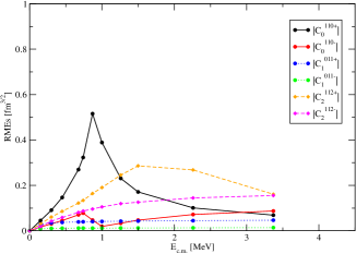
Figure 13: Same as in Fig. 11 bur for $P$-induced transitions.

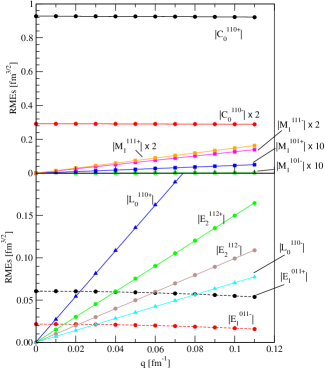
Figure 14: The dependence on the three-momentum transfer $q$ of some RMEs for the axial operators; the calculations are at incident proton energy of 0.9 MeV and use the N3LO500/N2LO500 chiral interactions. The solid (dashed) lines show fits of the calculated values using linear (quadratic) parametrizations. The RMEs not shown in this plot are negligible.

Lastly, in Figs. 14 and 15 we report the dependence on the three-momentum transfer $q$ of some of the RMEs associated with the axial- and pseudoscalar-exchange. Note that the RMEs associated with the pseudoscalar and time component of the axial operators behave differently, in particular $C_{0}^{110\pm}$ are $q$-independent and linear in $q$ in the axial and pseudoscalar case, respectively.

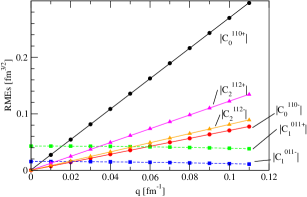
Figure 15: The same as in Fig. 14 but for the pseudoscalar operator

VII.2 Further comments on cross section results

Cross section results for the processes ³H$(p,e^{+}e^{-})^{4}$He and ³He$(n,e^{+}e^{-})^{4}$He have been presented and discussed in Sec. I.4. Here, we only report the values we have adopted for the isoscalar and isovector combinations, respectively $\eta^{c}_{0}$ and $\eta^{c}_{z}$, of coupling constants modulo the unknown $\varepsilon_{0}$ and $\varepsilon_{z}$,

$$\eta_{0}^{S}/\varepsilon_{0} = -4m_{\pi}^{2}c_{1}/\Lambda_{S}\approx 0.085\ ,$$

$$\eta_{z}^{S}/\varepsilon_{z} = -2m_{\pi}^{2}c_{5}/\Lambda_{S}\approx 0.00387\ ,$$

$$\eta_{0}^{P}/\varepsilon_{0} = 2m_{\pi}^{2}\,m_{N}(d_{18}+2\,d_{19})/\Lambda_{S}\approx 0.038\ ,$$

$$(g_{A}\,\eta_{z}^{P}/m_{\pi}f_{\pi})/\varepsilon_{z} = g_{A}m_{\pi}/\Lambda_{S}\approx 0.175\ ,$$

$$\eta_{0}^{V}/\varepsilon_{0} = 3\ ,$$ (119)

$$\eta_{z}^{V}/\varepsilon_{z} = 1\ ,\qquad$$

$$|\eta_{0}^{A}/\varepsilon_{0} = 3\,F-D\approx 0.55\ ,$$

$$\eta_{z}^{A}/\varepsilon_{z} = F+D\approx 1.25\ ,$$

see Eqs. (59), (64), (65), (72), and (89). The value of the LEC $c_{1}\,$=$\,-1.10$ GeV^-1 is taken from Ref. Hoferichter et al. (2016), where it has been extracted from an analysis of $\pi N$ scattering data. The value of the LEC $c_{5}$ is related to the $n$-$p$ mass difference $\delta m^{\rm str}$ induced by the strong interactions Bsaisou et al. (2015), that is, $c_{5}\,$=$\,\delta m^{\rm str}/(4\,B_{c}(m_{u}-m_{d})\,)\approx-9.9\times 10^{-2}$ GeV^-1. The values of $\delta m^{\rm str}$, and $m_{u}$ and $m_{d}$ are taken from Lattice QCD calculations Borsanyi et al. (2015); Walker-Loud (2014); Aoki et al. (2019). Note that $\eta^{S}_{z}/\varepsilon_{z}\ll\eta^{S}_{0}/\varepsilon_{0}$. The combination $\eta^{S}_{0}/\varepsilon_{0}$ is actually related to the so-called $\sigma_{\pi N}$ term, that is, $\eta^{S}_{0}/\varepsilon_{0}\,$=$\,\sigma_{\pi N}/\Lambda_{S}$. The adopted value is equivalent to approximating $\sigma_{\pi N}\,$=$\,-4m_{\pi}^{2}c_{1}$ which represents the LO contribution as determined in a $\chi$PT analysis Crivellin et al. (2014). Since this expansion is poorly convergent for $\sigma_{\pi N}$, perhaps a better approximation would be to use the empirical value, as derived from the analysis of $\pi N$ scattering data or directly from LQCD calculations (see, for example, Ref.  Ruiz de Elvira et al. (2018)). This would give a value for $\eta^{S}_{0}/\varepsilon_{0}\,$ that is about 30% smaller from that reported in Eq. (VII.2). The estimate for the pseudoscalar coupling constant $\eta_{0}^{P}$ follows from taking $m_{N}(d_{18}+2\,d_{19})\,$=$\,1$ GeV^-1, with $d_{18}\approx-1$ GeV^-2 from the Goldberger-Treiman discrepancy Fettes et al. (1998) and the poorly known $d_{19}\approx 1$ GeV^-2. Given that we have no knowledge of the coupling constants of the X17 to the electron and nucleon, the above uncertainties are unimportant at the present time.

In computing the four-fold differential cross section, special care must be exercised in carrying out the integration over the electron energy, particularly when the width $\Gamma_{X}$ of the X17 is small. The origin of this difficulty is easily understood. The interference and direct pieces of the cross section are proportional to powers of

$$\frac{1}{Q^{2}-M_{X}^{2}}\longrightarrow\frac{1}{Q^{2}-M_{X}^{2}+i\,M_{X}\,\Gamma_{X}}\equiv\frac{1}{D_{X}}\ ,$$ (120)

where it has been assumed $\Gamma_{X}^{2}\ll M_{X}^{2}$. When the lepton-pair kinematics is such that $Q^{2}\approx M_{X}^{2}$, the X17 propagator reduces to $-i/(M_{X}\Gamma_{X})$, and this behavior is at the origin of the peaks observed in the five-fold differential cross section for large $\theta_{ee}$. We elaborate on this aspect of the calculations in the following.

VII.2.1 Energy and angular dependence of the cross section

In general the five-fold differential cross section can be schematically written as (we only indicate explicitly the energy dependence)

$${d^{5}\sigma\over d\epsilon\,d\hat{\bm{k}}\,d\hat{\bm{k}}^{\prime}} = \sigma(\epsilon)+\varepsilon_{e}\left[{R_{X}(\epsilon)\over D_{X}}+{\rm c.c.}\right]+\varepsilon_{e}^{2}\,{R_{XX}(\epsilon)\over|D_{X}|^{2}}$$

$$= \sigma(\epsilon)+\frac{\varepsilon_{e}\left[R_{X}(\epsilon)\,D_{X}^{*}+{\rm c.c.}\right]+\varepsilon_{e}^{2}\,R_{XX}(\epsilon)}{|D_{X}|^{2}}\ ,$$

where $\sigma(\epsilon)$, $R_{X}(\epsilon)$, and $R_{XX}(\epsilon)$ denote, respectively, the purely electromagnetic term, the interference term between electromagnetic and X17-induced amplitudes, and the purely X17 term. Note that we have made explicit the dependence on the coupling constant $\varepsilon_{e}$.

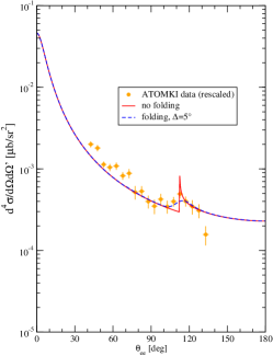
Figure 16: Example of the folding of the four-fold differential cross section for the process ${{}^{3}{\rm H}}(p,e^{-}e^{+}){{}^{4}{\rm He}}$ calculated with the N3LO500/N2LO500 Hamiltonian at an incident proton energy of 0.9 MeV.

Using the Lagrangians given in Eq. (2), the width of the X17 is obtained (in first-order perturbation theory) as

$$\Gamma^{S}_{X} = \alpha\,\varepsilon_{e}^{2}\,{M_{X}^{2}-4m_{e}^{2}\over 2M_{X}}\sqrt{1-{4\,m_{e}^{2}\over M_{X}^{2}}}\ ,$$

$$\Gamma^{P}_{X} = \alpha\,\varepsilon_{e}^{2}\,{M_{X}\over 2}\sqrt{1-{4\,m_{e}^{2}\over M_{X}^{2}}}\ ,$$

$$\Gamma^{V}_{X} = \alpha\,\varepsilon_{e}^{2}\,{M_{X}^{2}+2\,m_{e}^{2}\over 3\,M_{X}}\sqrt{1-{4\,m_{e}^{2}\over M_{X}^{2}}}\ ,$$ (122)

$$\Gamma^{A}_{X} = \alpha\,\varepsilon_{e}^{2}\,{M_{X}^{2}-4\,m_{e}^{2}\over 3\,M_{X}}\sqrt{1-{4\,m_{e}^{2}\over M_{X}^{2}}}\ .$$

In the limit $M_{X}^{2}\gg m_{e}^{2}$, the width $\Gamma^{c}_{X}$ reduces to

$$\Gamma^{c}_{X}=x_{c}\,\alpha\,\varepsilon_{e}^{2}\,M_{X}\equiv\varepsilon^{2}_{e}\,\gamma_{X}^{c}\ ,$$ (123)

where $x_{c}$ is a numerical factor of order unity. Available current bounds on $\varepsilon_{e}$ suggest $\Gamma_{X}^{c}\ll M_{X}$ Feng et al. (2016); Delle Rose et al. (2019b).

As noted in Sec. I.4, the condition $Q^{2}\,$=$\,M_{X}^{2}$ is satisfied by two different values, $\epsilon_{1}$ and $\epsilon_{2}$, of the electron energy, and according to Eq. (16) for $\epsilon$ close to $\epsilon_{i}$ we can approximate $1/|D_{X}|^{2}$ as

$$\frac{1}{|D_{X}|^{2}}\longrightarrow\frac{\pi}{|\alpha_{i}|}\,\frac{1}{\varepsilon_{e}^{2}\,\gamma^{c}_{X}\,M_{X}}\,\delta(\epsilon-\epsilon_{i})\ .$$ (124)

In such a limit, in the cross section of Eq. (VII.2.1), the interference and direct terms are proportional to $\delta(\epsilon-\epsilon_{i})$ with the electron energy argument evaluated at $\epsilon_{i}$. It is worthwhile pointing out here that in the direct term proportional to $R_{XX}$ the dependence on $\varepsilon_{e}^{2}$ is removed (of course, in the present tree-level treatment of the X17 width). It turns out that for $\varepsilon_{e}\approx 10^{-3}$ the interference contribution (proportional to $R_{X}$) is always negligible relative to the direct one.

In order to obtain the four-fold differential cross section, the integration over $\epsilon$ is carried out numerically for the electromagnetic term, and analytically for the interference and direct terms. We account roughly for the finite angular resolution of the detector employed in the experiment by folding the $\theta_{ee}$ dependence of this (four-fold) cross section with a normalized Gaussian of width $\Delta$. The cross sections plotted in Figs. 5 and 6 have been obtained in this way, using typical values of $\Delta$ around $3$–$5^{\circ}$. In Fig. 16, we show an example of a folded and non-folded cross section. In principle, we should have accounted for the finite resolution in the determination of the individual electron and positron angles $\theta$ and $\theta^{\prime}$ (rather than $\theta_{ee}$). However, in this first study we are not concerned with refinements such as this.

VII.2.2 Determining the X17 coupling constants from the 2019 ATOMKI data

We now turn our attention to the comparison with the ATOMKI data for the ${{}^{3}{\rm H}}(p,e^{+}e^{-}){{}^{4}{\rm He}}$ process at $E_{p}\,$=$\,0.90$ MeV Krasznahorkay et al. (2019). As noted earlier, the cross section is essentially independent of $\varepsilon_{e}$, but does depend on the mass $M_{X}$ and the coupling constants $\eta^{c}_{\alpha}$. We have taken $M_{X}\,$=$\,17$ MeV, while we have fixed the $\eta^{c}_{\alpha}$ by fitting the ATOMKI data in the peak region (the X17 contribution is negligible for $\theta_{ee}<90^{\circ}$) as follows: for $S$-exchange, we have determined only $\eta_{0}^{S}$, and have set $\eta^{S}_{z}\,$=$\,0$, since (i) this coupling constant, being proportional to the LEC $c_{5}$, is expected to be much smaller than $\eta_{0}^{S}$, and (ii) matrix elements of the isovector $S$ current are much smaller than those of the isoscalar one; for $P$ exchange, we have considered two possibilities: in the first, we have set $\eta^{P}_{0}\,$=$\,0$, and have determined the isovector coupling constant $\eta^{P}_{z}$ (this would be the leading-order contribution in $\chi$EFT), whereas in the second we have determined $\eta^{P}_{0}$ by setting $\eta^{P}_{z}\,$ to zero, in accordance with the piophobic hypothesis of Ref. Alves (2021); for $V$ exchange we have taken $\eta^{V}_{z}\,$=$\,-\eta_{0}^{V}$ (proto-phobic assumption) and have determined $\eta^{V}_{0}$; for $A$ exchange, we have determined $\eta_{0}^{A}$, while setting $\eta^{A}_{z}\,$=$\,0$, since isoscalar matrix elements of the $A$ current are much larger than isovector ones, see Figs. 11 and 12.

Table 9: Values of the coupling constants $\varepsilon_{0}$ and $\varepsilon_{z}$ obtained from the fit of the 2019 ATOMKI angular distribution Krasznahorkay et al. (2019) for the two Hamiltonians employed in the present paper. The electromagnetic amplitudes are calculated using the corresponding accompanying electromagnetic currents. The values in boldface have been fixed as discussed in the main text; furthermore, $M_{X}\,$=$\,17$ MeV and $\varepsilon_{e}\,$=$\,10^{-3}$. The relations between these parameters and the coupling constants $\eta^{c}_{\alpha}$ are given in Eqs. (59), (64), (65), (72), and (89). Note that the proto-phobic condition for the vector case is equivalent to requiring $3\,\varepsilon_{0}+\varepsilon_{z}\,$=$\,0$.

	N3LO500/N2LO500		NVIa/3NIa
Case	$\varepsilon_{0}$	$\varepsilon_{z}$	$\varepsilon_{0}$	$\varepsilon_{z}$
$S$	$0.86\times 10^{0}$	${\bm{0}}$	$0.75\times 10^{0}$	${\bm{0}}$
$P$	${\bm{0}}$	$5.06\times 10^{0}$	${\bm{0}}$	$4.82\times 10^{0}$
$P$	$2.55\times 10^{1}$	${\bm{0}}$	$2.72\times 10^{1}$	${\bm{0}}$
$V$	$2.56\times 10^{-3}$	$-{\bm{3}}\,{\bm{\varepsilon}}_{0}$	$2.66\times 10^{-3}$	$-{\bm{3}}\,{\bm{\varepsilon}}_{0}$
$A$	$2.58\times 10^{-3}$	${\bm{0}}$	$2.89\times 10^{-3}$	${\bm{0}}$

The values of the coupling constants resulting from the fits are reported in Table 9 for the two different Hamiltonian models (and accompanying electromagnetic currents), considered in the present work. Of course, these values depend on the choice of the parameter $\Delta$ of the Gaussian function used in the folding procedure (see above); those in the table correspond to a $\Delta$ of $5^{\circ}$. Nevertheless, Table 9 indicates that the model dependence is weak; indeed, the coupling constants vary at most of of about 10%. We have made no attempt to estimate the uncertainty coming from the fits to the experimental data.

VII.2.3 Comparing to previous determinations of the X17 coupling constants

Of course, the coupling constants reported in Table 9 are rather uncertain (they depend on the specific values assumed for $M_{X}$ and $\varepsilon_{e}$, on the uncertainties in the experimental data, on the unsubtracted background of EPC events, etc.). Nevertheless, here we compare them to previous determinations, where available. In Ref. Feng et al. (2016) the coupling constants $\epsilon_{u}$ and $\epsilon_{d}$, entering $V$ exchange, were obtained by fitting the branching ratio for the ${{}^{8}{\rm Be}}$ anomaly, with typical values of the order $\sim\,10^{-3}$. The values for $\epsilon_{u,d}\,$=$\,(\varepsilon_{0}\pm\varepsilon_{z})/2$ inferred from Table 9 are consistent (order of magnitude) with those reported in that work.

For the case of $A$ exchange, we can compare the results of our fit with the $\epsilon_{u,d}$ extracted in Ref. Kozaczuk et al. (2017) (again, from the ${{}^{8}{\rm Be}}$ anomaly); there, they were reported to be of order $10^{-5}$–$10^{-4}$. We find them to be at least one order of magnitude larger than in that work. However, it is worthwhile pointing out that matrix elements of the axial current, in particular its longitudinal component, between the $0^{-}$ and $0^{+}$ states in helium are suppressed by $q$ relative to those between the $1^{+}$ and $0^{+}$ states in beryllium. As a matter of fact, in helium these matrix elements are even smaller than those induced by the axial charge, see curves labeled $L_{0}^{110+}$ and $C_{0}^{110+}$ in Fig. 12, even though, at least nominally, the latter operator is subleading in the power counting of $\chi$EFT. This suppression might explain why the coupling constants extracted from the helium and beryllium data differ by such a large factor.

In reference to $P$ exchange, on the other hand, in the literature only the case of an isoscalar coupling is considered Delle Rose et al. (2019b); Alves (2021). From our fit to the 2019 ATOMKI data, the nucleon coupling constant, Eq. (65), is estimated to be $g^{P}_{0}\equiv e\,\eta_{0}^{P}\approx 0.3$, two orders of magnitude larger than obtained in Refs. Delle Rose et al. (2019b); Alves (2021). The origin of this difference in the estimates of $g^{P}_{0}$ is unclear at this point in time.

The exchange of a scalar X17 was already excluded by the analysis of the ${{}^{8}{\rm Be}}$ anomaly in Refs. Feng et al. (2016); Delle Rose et al. (2019b); we have been unable to find any estimates in literature.

We conclude that both the ${{}^{8}{\rm Be}}$ and ${{}^{4}{\rm He}}$ anomalies can be explained simultaneously by the exchange of a proto-phobic vector X17. For an axial X17 exchange, the coupling constants appear to be inconsistent with each other, proviso the cautionary note above. Clearly, these conclusions are somewhat uncertain, due to various assumptions we made in fitting the data. A better strategy would be to perform simulations of the experimental data by including all relevant contributions for each of the four possibilities, that the X17 be a $S$, $P$, $V$, and $A$ boson. Work along these lines is in progress Krasznahorkay et al. (2021b).

VII.2.4 Comparing to the 2021 ATOMKI data

In this brief section we provide a preliminary analysis of the 2021 ${{}^{3}{\rm H}}(p,e^{+}e^{-}){{}^{4}{\rm He}}$ data by the ATOMKI group Krasznahorkay et al. (2021a). As noted earlier, in this new publication the authors also report background-free data (i.e., data from which EPC spurious events have been subtracted out). Unfortunately, these data have rather large errors, especially at smaller angles ($\theta_{ee}\lesssim 90^{\circ}$). On a more positive note, however, measurements are carried out at three different beam energies, thus permitting a first test of how the assumed nature for the X17 boson would impact the energy dependence of the peak structure, see Fig. 17.

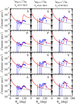
Figure 17: The four-fold differential cross section for the ${{}^{3}{\rm H}}(p,e^{-}e^{+}){{}^{4}{\rm He}}$ process at three different incident nucleon energies for the configuration in which the $e^{+}$ and $e^{-}$ momenta are in the plane orthogonal to the incident nucleon momentum and as function of the angle $\theta_{ee}$ between them, compared with the 2021 data of the ATOMKI group Krasznahorkay et al. (2021a). Notation as in Fig. 5. The coupling constants for the $S$, piophobic $P$, protophobic $V$, and $A$ X17 boson have been fixed by reproducing the data at $E_{p}\,$=$\,0.90$ MeV.

In this figure, the coupling constants for the $S$ (with $\eta_{z}^{S}\,$=$\,0$), piophobic $P$, proto-phobic $V$, and $A$ (with $\eta_{z}^{A}\,$=$\,0$) exchange have been fixed by reproducing the data at $E_{p}\,$=$\,0.90$ MeV. The results at $E_{p}\,$=$\,0.51$ and $0.61$ MeV are therefore predictions, and seem to better reproduce the corresponding data when the X17 is either a pseudoscalar or an axial boson. As the energy decreases, the prominence of the peak relative to the baseline of $e^{+}$-$e^{-}$ pairs produced by purely electromagnetic transitions is reduced, suggesting that the relevant matrix element may be that connecting the $0^{-}$ resonance to the ${{}^{4}{\rm He}}$ ground state. However, we note that (i) the large errors in the experimental data at $E_{p}\,$=$\,0.90$ MeV render problematic the matching of these data to the photon-only cross sections, and (ii) the coupling constants extracted from the present fit are much larger (in absolute value) than those reported in Table 9. In view of these considerations, we do not list these values here.

In conclusion, in order to clarify the present situation, we believe it would be very helpful to have more accurate measurements of these pair-production cross sections, by performing experimental studies in a wider range of energy and $e^{+}$-$e^{-}$ angles, as outlined in Sec. I.5.

Appendix A Chiral Lagrangians

The QCD Lagrangian ${\cal L}_{q}(x)$ in the $SU(2)$ formulation with up and down quark flavors and including couplings to external scalar, pseudoscalar, and vector sources is written as

$$\mathcal{L}_{q}(x) = \mathcal{L}_{q}^{0}(x)+\overline{q}(x)\,\gamma^{\mu}\left[v_{\mu}(x)+\frac{1}{3}\,v_{\mu}^{s}(x)\right]q(x)$$ (125)

$$- \overline{q}(x)[s(x)-i\gamma^{5}\,p(x)]q(x)\ ,$$

where $\mathcal{L}_{q}^{0}(x)$ is the Lagrangian for massless quarks, $q(x)$ is the two-component flavor vector

$$q(x)=\left[\!\begin{array}[]{c}u(x)\\ d(x)\end{array}\!\right]\ ,$$ (126)

and $u(x)$ and $d(x)$ are the up and down quark fields, respectively. The external scalar, pseudoscalar, and vector sources $s(x)$, $p(x)$, and $v_{\mu}(x)$ have the flavor (or isospin) structure

$$s(x)=\sum_{i=0}^{3}\tau_{i}\,s_{i}(x)\ ,\qquad p(x)=\sum_{i=0}^{3}\tau_{i}\,p_{i}(x)\ ,$$ (127)

and

$$v_{\mu}(x)=\sum_{i=1}^{3}\tau_{i}\,v_{\mu,i}(x)\ ,$$ (128)

where $\tau_{0}$ is the identity matrix (in isospin space) and $\tau_{i}$ are standard Pauli matrices. The external (isoscalar) vector source $v_{\mu}^{s}(x)$ is multiplied by the identity matrix $\tau_{0}$. Quark masses are reintroduced as part of the scalar source $s(x)=M_{q}+\cdots$ via

$$M_{q}=\left(\begin{array}[]{cc}m_{u}&0\\ 0&m_{d}\end{array}\right)=m_{q}\,\tau_{0}+\delta m_{q}\,\tau_{3}\ ,$$ (129)

where $m_{q}=(m_{u}+m_{d})/2$ and $\delta m_{q}=(m_{u}-m_{d})/2$, and $m_{u}$ and $m_{d}$ are the up- and down-quark mass, respectively.

The chiral Lagrangian ${\cal L}_{\chi}(x)$ consists of terms ${\cal L}_{\pi\pi}(x)$ and ${\cal L}_{\pi N}(x)$ describing, respectively, the interactions of pions and those of pions with nucleons. These terms have the expansions

$${\cal L}_{\pi\pi}(x) = {\cal L}_{\pi\pi}^{(2)}(x)+\cdots\ ,$$ (130)

$${\cal L}_{\pi N}(x) = {\cal L}_{\pi N}^{(1)}(x)+{\cal L}_{\pi N}^{(2)}(x)+{\cal L}_{\pi N}^{(3)}(x)+\cdots\ ,$$ (131)

where

$${\cal L}_{\pi\pi}^{(2)} = {f_{\pi}^{2}\over 4}\langle\nabla_{\mu}U^{\dagger}\nabla^{\mu}U+\chi^{\dagger}U+\chi U^{\dagger}\rangle\ ,$$ (132)

$${\cal L}_{\pi N}^{(1)} = \overline{N}\Bigl{(}i\gamma^{\mu}D_{\mu}-m_{N}\,\tau_{0}+{g_{A}\over 2}\gamma^{\mu}\gamma^{5}u_{\mu}\Bigr{)}N\ ,$$ (133)

$${\cal L}_{\pi N}^{(2)} = \overline{N}\Bigl{(}c_{1}\langle\chi_{+}\rangle+\cdots+c_{5}\hat{\chi}+{\kappa_{z}\over 8\,m_{N}}\sigma^{\mu\nu}F_{\mu\nu}^{+}$$ (134)

$$\quad+{\kappa_{0}\over 4\,m_{N}}\sigma^{\mu\nu}F_{\mu\nu}^{s}+\cdots\Bigr{)}N\ ,$$

$${\cal L}_{\pi N}^{(3)} = \cdots+i\,{d_{18}\over 2}\,\overline{N}\,\gamma^{\mu}\gamma^{5}[D_{\mu}\,,\,\chi_{-}]\,N$$ (135)

$$\quad+i\,{d_{19}\over 2}\,\overline{N}\,\gamma^{\mu}\gamma^{5}[D_{\mu}\,,\,\langle\chi_{-}\rangle]\,N+\cdots\ ,$$

where $f_{\pi}\approx 92.4$ MeV is the pion decay constant, $g_{A}=1.26$ is the nucleon axial coupling constant, $m_{N}$ is the nucleon mass, $\langle\cdots\rangle$ denotes a trace over isospin, and $\hat{\chi}=\chi-\langle\chi\rangle/2$. The isotriplet of pion fields is denoted below with ${\bm{\pi}}(x)$, while the isodoublet nucleon field $N(x)$ is given by

$$N(x)=\left[\begin{array}[]{c}p(x)\\ n(x)\end{array}\right]\ .$$ (136)

In the previous expressions we have omitted terms not relevant in the present work; the complete ${\cal L}_{\pi\pi}^{(4)}$ can be found in Ref. Gasser and Leutwyler (1984), and the complete ${\cal L}_{\pi N}^{(2)}$ and successive term in Ref. Fettes et al. (2000). Here, we adopt the notation and conventions of this latter work for the various fields and covariant derivatives, which we summarize below:

$$U = 1+{i\over f_{\pi}}{\bm{\tau}}\cdot{\bm{\pi}}-{1\over 2f_{\pi}^{2}}\,{\bm{\pi}}^{2}+\cdots\ ,$$

$$\nabla_{\mu}U = \partial_{\mu}U-i\,r_{\mu}\,U+i\,U\,\ell_{\mu}\ ,$$

$$u = \sqrt{U}\ ,$$

$$D_{\mu}N = (\partial_{\mu}+\Gamma_{\mu}-i\,v_{\mu}^{s})\,N\ ,$$

$$u_{\mu} = i(u^{\dagger}\partial_{\mu}u-u\,\partial_{\mu}u^{\dagger})+u^{\dagger}r_{\mu}u-u\,\ell_{\mu}u^{\dagger}\ ,$$ (137)

$$\Gamma_{\mu} = {1\over 2}(u^{\dagger}\partial_{\mu}u+u\,\partial_{\mu}u^{\dagger})-\frac{i}{2}(u^{\dagger}r_{\mu}u+u\,\ell_{\mu}u^{\dagger})\ ,$$

$$\chi_{\pm} = u^{\dagger}\chi\,u^{\dagger}\pm u\,\chi^{\dagger}u\ ,$$

$$F_{\mu\nu}^{\pm} = u^{\dagger}\,F_{\mu\nu}^{R}\,u\pm u\,F_{\mu\nu}^{L}\,u^{\dagger}\ .$$

For the cases of interest in the present work, we have

$$r_{\mu} = \ell_{\mu}=v_{\mu}\ ,\quad\chi=2\,B_{c}\,(s+ip)\ ,$$

$$F_{\mu\nu}^{R} = F_{\mu\nu}^{L}=\partial_{\mu}v_{\nu}-\partial_{\nu}v_{\mu}-i\,[v_{\mu}\,,\,v_{\nu}]\ ,$$ (138)

$$F_{\mu\nu}^{s} = \partial_{\mu}v_{\nu}^{s}-\partial_{\nu}v_{\mu}^{s}\ ,$$

The parameters $B_{c}$, $c_{1}$, etc., entering the Lagrangians are the so-called low energy constants (LECs), to be determined from experimental data and/or (possibly) lattice QCD calculations.

The nucleon and pion fields (in interaction picture) read

$$N_{t}(x) = \sum_{{\bm{p}}s}{1\over\sqrt{\Omega}}\Bigl{[}b_{{\bm{p}}st}\,u_{{\bm{p}}s}\,e^{-ip\cdot x}+d_{{\bm{p}}st}^{\dagger}\,v_{{\bm{p}}s}\,e^{ip\cdot x}\Bigr{]}\ ,$$

$$\pi_{a}(x) = \sum_{{\bm{k}}}{1\over\sqrt{2\omega_{k}\,\Omega}}\Bigl{[}a_{{\bm{k}}a}\,e^{-ik\cdot x}+a_{{\bm{k}}a}^{\dagger}\,e^{ik\cdot x}\Bigr{]}\ ,$$ (139)

where the various momenta are discretized by assuming periodic boundary conditions in a box of volume $\Omega$, $b_{{\bm{p}}st}$ and $d_{{\bm{p}}st}$ are the annihilation operators of, respectively, a nucleon and antinucleon having spin and isospin projections $s$ and $t$ ($t\,$=$\,1/2$ for a proton and $t\,$=$\,-1/2$ for a neutron), $u$ and $v$ are the corresponding Dirac spinors with the (non-standard) normalization $u^{\dagger}u\,$=$\,v^{\dagger}v\,$=$\,1$, and $a_{{\bm{k}}a}$ is the annihilation operator of a pion of isospin projection $a$.

References

- Battaglieri et al. (2017) M. Battaglieri et al., in U.S . Cosmic Visions: New Ideas in Dark Matter (2017) arXiv:1707.04591 [hep-ph] .
- Bertone and Hooper (2018) G. Bertone and D. Hooper, Rev. Mod. Phys. 90, 045002 (2018).
- Krasznahorkay et al. (2016) A. J. Krasznahorkay et al., Phys. Rev. Lett. 116, 042501 (2016), arXiv:1504.01527 [nucl-ex] .
- Pospelov et al. (2008) M. Pospelov, A. Ritz, and M. Voloshin, Physics Letters B 662, 53 (2008).
- Banerjee et al. (2018) D. Banerjee et al. (NA64), Phys. Rev. Lett. 120, 231802 (2018), arXiv:1803.07748 [hep-ex] .
- Batley et al. (2015) J. Batley et al. (NA48/2), Phys. Lett. B 746, 178 (2015), arXiv:1504.00607 [hep-ex] .
- Andreas et al. (2010) S. Andreas, O. Lebedev, S. Ramos-Sanchez, and A. Ringwald, J.High Energ. Phys. 2010, 3 (2010), arXiv:1005.3978 [hep-ph] .
- Feng et al. (2016) J. L. Feng, B. Fornal, I. Galon, S. Gardner, J. Smolinsky, T. M. P. Tait, and P. Tanedo, Phys. Rev. Lett. 117, 071803 (2016), arXiv:1604.07411 [hep-ph] .
- Kozaczuk et al. (2017) J. Kozaczuk, D. E. Morrissey, and S. Stroberg, Phys. Rev. D 95, 115024 (2017), arXiv:1612.01525 [hep-ph] .
- Krasznahorkay et al. (2019) A. Krasznahorkay et al., (2019), arXiv:1910.10459 [nucl-ex] .
- Krasznahorkay et al. (2021a) A. J. Krasznahorkay, M. Csatlós, L. Csige, J. Gulyás, A. Krasznahorkay, B. M. Nyakó, I. Rajta, J. Timár, I. Vajda, and N. J. Sas, (2021a), arXiv:2104.10075 [nucl-ex] .
- Feng et al. (2020) J. L. Feng, T. M. Tait, and C. B. Verhaaren, Phys. Rev. D 102, 036016 (2020), arXiv:2006.01151 [hep-ph] .
- Zhang and Miller (2021) X. Zhang and G. A. Miller, Physics Letters B 813, 136061 (2021), arXiv:2008.11288 [hep-ph] .
- Hayes et al. (2021) A. C. Hayes, J. L. Friar, G. Hale, and G. Garvey, (2021), arXiv:2106.06834 [nucl-th] .
- Andreas et al. (2012) S. Andreas, C. Niebuhr, and A. Ringwald, Phys. Rev. D 86, 095019 (2012).
- Riordan et al. (1987) E. M. Riordan, M. W. Krasny, K. Lang, P. de Barbaro, A. Bodek, S. Dasu, N. Varelas, X. Wang, R. Arnold, D. Benton, P. Bosted, L. Clogher, A. Lung, S. Rock, Z. Szalata, B. W. Filippone, R. C. Walker, J. D. Bjorken, M. Crisler, A. Para, J. Lambert, J. Button-Shafer, B. Debebe, M. Frodyma, R. S. Hicks, G. A. Peterson, and R. Gearhart, Phys. Rev. Lett. 59, 755 (1987).
- Anastasi et al. (2015) A. Anastasi et al., Phys. Lett. B 750, 633 (2015), arXiv:1509.00740 [hep-ex] .
- Abi et al. (2021) B. Abi et al. (Muon g-2), Phys. Rev. Lett. 126, 141801 (2021), arXiv:2104.03281 [hep-ex] .
- Borsanyi et al. (2021) S. Borsanyi, Z. Fodor, J. Guenther, C. Hoelbling, S. Katz, L. Lellouch, T. Lippert, K. Miura, L. Parato, K. Szabo, F. Stokes, B. Toth, C. Torok, and L. Varnhorst, Nature 593, 51—55 (2021).
- Fayet (2007) P. Fayet, Phys. Rev. D 75, 115017 (2007).
- Morel et al. (2020) L. Morel, Z. Yao, P. Cladé, and S. Guellati-Khélifa, Nature 588, 61 (2020).
- Zhang and Miller (2017) X. Zhang and G. A. Miller, Phys. Lett. B 773, 159 (2017), arXiv:1703.04588 [nucl-th] .
- Ellwanger and Moretti (2016) U. Ellwanger and S. Moretti, J. High Energ. Phys. 2016, 39 (2016), arXiv:1609.01669 [hep-ph] .
- Dror et al. (2017) J. A. Dror, R. Lasenby, and M. Pospelov, Phys. Rev. Lett. 119, 141803 (2017), arXiv:1705.06726 [hep-ph] .
- Delle Rose et al. (2017) L. Delle Rose, S. Khalil, and S. Moretti, Phys. Rev. D 96, 115024 (2017), arXiv:1704.03436 [hep-ph] .
- Delle Rose et al. (2019a) L. Delle Rose, S. Khalil, S. J. King, S. Moretti, and A. M. Thabt, Phys. Rev. D 99, 055022 (2019a), arXiv:1811.07953 [hep-ph] .
- Delle Rose et al. (2019b) L. Delle Rose, S. Khalil, S. J. King, and S. Moretti, Front. in Phys. 7, 73 (2019b), arXiv:1812.05497 [hep-ph] .
- Alves and Weiner (2018) D. S. M. Alves and N. Weiner, JHEP 07, 092 (2018), arXiv:1710.03764 [hep-ph] .
- Alves (2021) D. S. M. Alves, Phys. Rev. D 103, 055018 (2021), arXiv:2009.05578 [hep-ph] .
- Bordes et al. (2019) J. Bordes, H.-M. Chan, and S. T. Tsou, Int. J. Mod. Phys. A 34, 1950140 (2019), arXiv:1906.09229 [hep-ph] .
- Nam (2020) C. H. Nam, Eur. Phys. J. C 80, 231 (2020), arXiv:1907.09819 [hep-ph] .
- Kirpichnikov et al. (2020) D. Kirpichnikov, V. E. Lyubovitskij, and A. S. Zhevlakov, Phys. Rev. D 102, 095024 (2020), arXiv:2002.07496 [hep-ph] .
- Fayet (2021) P. Fayet, Physical Review D 103, 035034 (2021), arXiv:2010.04673 [hep-ph] .
- Fornal (2017) B. Fornal, Int. J. Mod. Phys. A 32, 1730020 (2017), arXiv:1707.09749 [hep-ph] .
- Baldini et al. (2018) A. M. Baldini et al. (MEG II), Eur. Phys. J. C 78, 380 (2018), arXiv:1801.04688 [physics.ins-det] .
- Balewski et al. (2014) J. Balewski et al. (2014) arXiv:1412.4717 [physics.ins-det] .
- Ahdida et al. (2020) C. Ahdida et al. (SHiP), (2020), arXiv:2010.11057 [hep-ex] .
- Kou et al. (2019) E. Kou, P. Urquijo, W. Altmannshofer, et al. (Belle-II), Prog. Theor. Exp. Phys. 2019, 123C01 (2019), [Erratum: PTEP 2020, 029201 (2020)], arXiv:1808.10567 [hep-ex] .
- Banerjee et al. (2020) D. Banerjee, J. Bernhard, V. E. Burtsev, A. G. Chumakov, D. Cooke, P. Crivelli, E. Depero, A. V. Dermenev, S. V. Donskov, R. R. Dusaev, T. Enik, N. Charitonidis, A. Feshchenko, V. N. Frolov, A. Gardikiotis, S. G. Gerassimov, S. N. Gninenko, M. Hösgen, M. Jeckel, V. A. Kachanov, A. E. Karneyeu, G. Kekelidze, B. Ketzer, D. V. Kirpichnikov, M. M. Kirsanov, V. N. Kolosov, I. V. Konorov, S. G. Kovalenko, V. A. Kramarenko, L. V. Kravchuk, N. V. Krasnikov, S. V. Kuleshov, V. E. Lyubovitskij, V. Lysan, V. A. Matveev, Y. V. Mikhailov, L. Molina Bueno, D. V. Peshekhonov, V. A. Polyakov, B. Radics, R. Rojas, A. Rubbia, V. D. Samoylenko, D. Shchukin, V. O. Tikhomirov, I. Tlisova, D. A. Tlisov, A. N. Toropin, A. Y. Trifonov, B. I. Vasilishin, G. Vasquez Arenas, P. V. Volkov, V. Y. Volkov, and P. Ulloa (The NA64 Collaboration), Phys. Rev. D 101, 071101 (2020).
- Tilley et al. (1992) D. R. Tilley, H. R. Weller, and G. M. Hale, Nucl. Phys. A 541, 1 (1992).
- Kálmán and Keszthelyi (2020) P. Kálmán and T. Keszthelyi, Eur. Phys. J. A 56, 205 (2020), arXiv:2005.10643 [nucl-th] .
- Aleksejevs et al. (2021) A. Aleksejevs, S. Barkanova, Y. G. Kolomensky, and B. Sheff, (2021), arXiv:2102.01127 [hep-ph] .
- Koch (2021) B. Koch, Nucl. Phys. A 1008, 122143 (2021), arXiv:2003.05722 [hep-ph] .
- Viviani et al. (2020) M. Viviani, L. Girlanda, A. Kievsky, and L. E. Marcucci, Phys. Rev. C 102, 034007 (2020), arXiv:2003.14059 [nucl-th] .
- Entem and Machleidt (2003) D. Entem and R. Machleidt, Phys. Rev. C 68, 041001 (2003), arXiv:nucl-th/0304018 .
- Machleidt and Entem (2011) R. Machleidt and D. R. Entem, Phys. Rept. 503, 1 (2011), arXiv:1105.2919 [nucl-th] .
- Epelbaum et al. (2002) E. Epelbaum, A. Nogga, W. Gloeckle, H. Kamada, U.-G. Meissner, and H. Witala, Phys. Rev. C 66, 064001 (2002), arXiv:0208023 [nucl-th] .
- Piarulli et al. (2016) M. Piarulli, L. Girlanda, R. Schiavilla, A. Kievsky, A. Lovato, L. E. Marcucci, S. C. Pieper, M. Viviani, and R. B. Wiringa, Phys. Rev. C 94, 054007 (2016), arXiv:1606.06335 [nucl-th] .
- Piarulli et al. (2018) M. Piarulli et al., Phys. Rev. Lett. 120, 052503 (2018), arXiv:1707.02883 [nucl-th] .
- Pastore et al. (2008) S. Pastore, R. Schiavilla, and J. L. Goity, Phys. Rev. C 78, 064002 (2008), arXiv:0810.1941 [nucl-th] .
- Pastore et al. (2009) S. Pastore, L. Girlanda, R. Schiavilla, M. Viviani, and R. Wiringa, Phys. Rev. C 80, 034004 (2009), arXiv:0906.1800 [nucl-th] .
- Pastore et al. (2011) S. Pastore, L. Girlanda, R. Schiavilla, and M. Viviani, Phys. Rev. C 84, 024001 (2011), arXiv:1106.4539 [nucl-th] .
- Koelling et al. (2009) S. Koelling, E. Epelbaum, H. Krebs, and U.-G. Meissner, Phys. Rev. C 80, 045502 (2009), arXiv:0907.3437 [nucl-th] .
- Koelling et al. (2011) S. Koelling, E. Epelbaum, H. Krebs, and U.-G. Meissner, Phys. Rev. C 84, 054008 (2011), arXiv:1107.0602 [nucl-th] .
- Piarulli et al. (2013) M. Piarulli, L. Girlanda, L. E. Marcucci, S. Pastore, R. Schiavilla, and M. Viviani, Phys. Rev. C 87, 014006 (2013), arXiv:1212.1105 [nucl-th] .
- Schiavilla et al. (2019) R. Schiavilla et al., Phys. Rev. C 99, 034005 (2019), arXiv:1809.10180 [nucl-th] .
- Bacca and Pastore (2014) S. Bacca and S. Pastore, J. Phys. G 41, 123002 (2014), arXiv:1407.3490 [nucl-th] .
- Carlson et al. (2015) J. Carlson, S. Gandolfi, F. Pederiva, S. C. Pieper, R. Schiavilla, K. E. Schmidt, and R. B. Wiringa, Rev. Mod. Phys. 87, 1067 (2015), arXiv:1412.3081 [nucl-th] .
- Marcucci et al. (2016) L. E. Marcucci, F. Gross, M. T. Pena, M. Piarulli, R. Schiavilla, I. Sick, A. Stadler, J. W. Van Orden, and M. Viviani, J. Phys. G 43, 023002 (2016), arXiv:1504.05063 [nucl-th] .
- Perry and Bame (1955) J. E. Perry and S. J. Bame, Phys. Rev. 99, 1368 (1955).
- Hahn et al. (1995) K. I. Hahn, C. R. Brune, and R. W. Kavanagh, Phys. Rev. C 51, 1624 (1995).
- Canon et al. (2002) R. S. Canon, S. O. Nelson, K. Sabourov, E. Wulf, H. R. Weller, R. M. Prior, M. Spraker, J. H. Kelley, and D. R. Tilley, Phys. Rev. C 65, 044008 (2002).
- Komar et al. (1993) R. J. Komar, H.-B. Mak, J. R. Leslie, H. C. Evans, E. Bonvin, E. D. Earle, and T. K. Alexander, Phys. Rev. C 48, 2375 (1993).
- Kievsky et al. (2008) A. Kievsky, S. Rosati, M. Viviani, L. Marcucci, and L. Girlanda, J. Phys. G 35, 063101 (2008), arXiv:0805.4688 [nucl-th] .
- Marcucci et al. (2020) L. E. Marcucci, J. Dohet-Eraly, L. Girlanda, A. Gnech, A. Kievsky, and M. Viviani, Front. in Phys. 8, 69 (2020), arXiv:1912.09751 [nucl-th] .
- Schiavilla et al. (1989) R. Schiavilla, V. R. Pandharipande, and D.-O. Riska, Phys. Rev. C 40, 2294 (1989).
- Gustavino et al. (2021) C. Gustavino et al., PRIN2020.0004062.26-01-2021, unpublished (2021).
- Sabaté-Gilarte et al. (2017) M. Sabaté-Gilarte et al., Eur. Phys. J. A 53, 210 (2017).
- Baroni et al. (2018) A. Baroni et al., Phys. Rev. C 98, 044003 (2018), arXiv:1806.10245 [nucl-th] .
- Viviani et al. (2011) M. Viviani, A. Deltuva, R. Lazauskas, J. Carbonell, A. Fonseca, A. Kievsky, L. E. Marcucci, and S. Rosati, Phys. Rev. C 84, 054010 (2011), arXiv:1109.3625 [nucl-th] .
- Viviani et al. (2017) M. Viviani, A. Deltuva, R. Lazauskas, A. Fonseca, A. Kievsky, and L. E. Marcucci, Phys. Rev. C 95, 034003 (2017), arXiv:1610.09140 [nucl-th] .
- Kegel et al. (2021) S. Kegel et al., in preparation (2021).
- Piarulli et al. (2014) M. Piarulli, L. Girlanda, L. Marcucci, S. Pastore, R. Schiavilla, and M. Viviani, PoS Bormio2014, 040 (2014).
- Walecka (1995) J. D. Walecka, Theoretical Nuclear and Subnuclear Physics (Oxford University Press, New York, 1995).
- Marcucci et al. (2001) L. E. Marcucci, R. Schiavilla, M. Viviani, A. Kievsky, S. Rosati, and J. F. Beacom, Phys. Rev. C 63, 015801 (2001), arXiv:nucl-th/0006005 .
- Schiavilla and Wiringa (2002) R. Schiavilla and R. B. Wiringa, Phys. Rev. C 65, 054302 (2002).
- Edmonds (1957) A. Edmonds, Angular Momentum in Quantum Mechanics (Princeton University Press, Princeton, 1957).
- Siegert (1937) A. J. F. Siegert, Phys. Rev. 52, 787 (1937).
- Peskin and Schroeder (1995) M. E. Peskin and D. V. Schroeder, An Introduction to quantum field theory (Addison-Wesley, Reading, USA, 1995).
- Scherer and Schindler (2005) S. Scherer and M. R. Schindler, (2005), arXiv:hep-ph/0505265 .
- Green et al. (2017) J. Green, N. Hasan, S. Meinel, M. Engelhardt, S. Krieg, J. Laeuchli, J. Negele, K. Orginos, A. Pochinsky, and S. Syritsyn, Phys. Rev. D 95, 114502 (2017), arXiv:1703.06703 [hep-lat] .
- Weinberg (1995) S. Weinberg, The Quantum Theory of Fields (Cambridge University Press, New York, 1995).
- Hoferichter et al. (2016) M. Hoferichter, J. Ruiz de Elvira, B. Kubis, and U.-G. Meißner, Phys. Rept. 625, 1 (2016), arXiv:1510.06039 [hep-ph] .
- Bsaisou et al. (2015) J. Bsaisou, U.-G. Meißner, A. Nogga, and A. Wirzba, Annals Phys. 359, 317 (2015), arXiv:1412.5471 [hep-ph] .
- Borsanyi et al. (2015) S. Borsanyi et al., Science 347, 1452 (2015), arXiv:1406.4088 [hep-lat] .
- Walker-Loud (2014) A. Walker-Loud, PoS LATTICE2013, 013 (2014), arXiv:1401.8259 [hep-lat] .
- Aoki et al. (2019) S. Aoki et al. (Flavour Lattice Averaging Group), (2019), arXiv:1902.08191 [hep-lat] .
- Crivellin et al. (2014) A. Crivellin, M. Hoferichter, and M. Procura, Phys. Rev. D 89, 054021 (2014), arXiv:1312.4951 [hep-ph] .
- Ruiz de Elvira et al. (2018) J. Ruiz de Elvira, M. Hoferichter, B. Kubis, and U.-G. Meißner, J. Phys. G 45, 024001 (2018), arXiv:1706.01465 [hep-ph] .
- Fettes et al. (1998) N. Fettes, U.-G. Meissner, and S. Steininger, Nucl. Phys. A 640, 199 (1998), arXiv:hep-ph/9803266 .
- Krasznahorkay et al. (2021b) A. J. Krasznahorkay et al., in preparation (2021b).
- Gasser and Leutwyler (1984) J. Gasser and H. Leutwyler, Annals Phys. 158, 142 (1984).
- Fettes et al. (2000) N. Fettes, U.-G. Meißner, M. Mojzis, and S. Steininger, Annals Phys. 283, 273 (2000), [Erratum: Annals Phys. 288, 249–250 (2001)], arXiv:hep-ph/0001308 .