Exploring Visual Engagement Signals for Representation Learning

Abstract

Visual engagement in social media platforms comprises interactions with photo posts including comments, shares, and likes. In this paper, we leverage such Visual Engagement clues as supervisory signals for representation learning. However, learning from engagement signals is non-trivial as it is not clear how to bridge the gap between low-level visual information and high-level social interactions. We present VisE, a weakly supervised learning approach, which maps social images to pseudo labels derived by clustered engagement signals. We then study how models trained in this way benefit subjective downstream computer vision tasks such as emotion recognition or political bias detection. Through extensive studies, we empirically demonstrate the effectiveness of VisE across a diverse set of classification tasks beyond the scope of conventional recognition .

1 Introduction

People post photos on social media to invite engagement and seek connections. A photo of a cute dog can resonate with other dog lovers and trigger reactions such as the “like” or “love” button or comments including “what an adorable dog” and “look at those blue eyes!” The widely available interactions with the photos posted on social media, which we call visual engagement, contain rich semantic descriptions (“dog”, “blue eyes”) and are far less expensive to obtain than manual annotations in standard computer vision tasks, including coarse and fine-grained class labels [11, 80, 95], bounding boxes [51, 23], and image captions [8].

More importantly, visual engagement, including comments, replies, likes, and shares, provides emotional and cultural context that goes beyond the image content therein. For example, the image in Fig. 1 could be described in a standard captioning task as “a dog sits next to a stuffed animal.” The social media audience of this post may react to the cuteness of the dog, comment on the torn stuffed animal with whimsical responses, or initiate a conversation. The resulting textual descriptions depart from the exactly what it says on the tin approach of standard image captioning tasks and express private states [65, 82]: opinions, emotions, and speculations, for example. We argue that visual engagement can also serve as supervisory signals for representation learning and transfer well to subjective downstream computer vision tasks like emotion recognition or political bias classification.

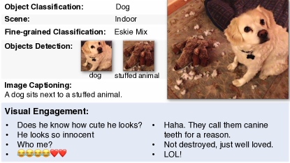
Figure 1: Visual engagement vs. other common supervisory signals. Given the same image, visual engagement provide semantically and contextually richer information than conventional recognition and captioning tasks.

Motivated by this observation, we propose to learn image representations from semantically and contextually rich Visual Engagement signals (VisE). We hypothesize that such learned representations, as a byproduct of mapping image content to human reactions, are able to infer private states expressed by images. This is beneficial and could serve as a nice addition to current computer vision research which in general focuses on the objectively present factual information from images (e.g., “this is a dog” vs. “what a cute dog!”).

Open-world visual engagement contains dense subjectivity clues, but is inherently noisy in nature. How to properly leverage such signals for representation learning is a challenging, open question. Inspired by recent studies on feature learning from proxy tasks [19, 3, 84], we cluster each type of visual engagement and obtain cluster assignment indices for all the responses associated with a training image. These cluster assignments are used as supervisory cues. We then train a network from scratch to map images to cluster assignments in a multi-task fashion for representation learning, where each task is to predict the cluster index for that type of response. In this paper, we consider two forms of human responses: (1) comments and (2) reactions. In the former case, we conduct the clustering on representations encoded by a textual model. Unlike most existing multi-modal methods that perform pre-training for both language and vision modules [12, 66] with hundreds of millions of parameters, we simply use an off-the-shelf encoder to embed comments, which is computationally efficient. We then evaluate representations learned from engagement signals on downstream tasks.

Our main contribution is to demonstrate that social media engagement can provide supervision for learning image representations that benefit subjective downstream tasks. To this end, we explore VisE pre-trained on 250 million publicly available social media posts. Through extensive experiments, we show that in three downstream tasks related to private states detection, the learned VisE models can outperform the ImageNet-supervised counterpart by a substantial margin in some cases. These results highlight that VisE broadens the current representation learning paradigms, thereby narrowing the gap between machine and human intelligence.

2 Related Work

Visual representation learning Learning discriminative features for targeted datasets is a core problem for many computer vision research efforts. Feature learning on small datasets is particularly difficult since high-capacity deep neural networks suffer from overfitting when the amount of target training data is limited. One popular way to mitigate this issue is to pre-train on large-scale image datasets with manually curated class labels such as ImageNet and COCO [13, 15]. However, training on ImageNet requires manually labeled data, which are expensive to obtain and hard to scale. This motivates a plethora of work investigating weakly-supervised [73, 55, 41, 42, 47], semi-supervised [86, 87, 84] and self-supervised learning [3, 96, 14, 4, 22, 48, 90]. These methods tap into alternative forms of supervision, such as user-provided tags [76, 55] and hand-crafted pretext tasks (e.g., inpainting [64], colorization [91, 92], predicting jigsaw permutations [60], rotations of inputs [17]). More recently, contrastive learning [24, 25] is used for feature learning by bringing images closer to their augmented versions than other samples in the training set [83, 89, 26, 58, 6]. In this paper, we use visual engagement, which encompasses high-level semantics, as supervisory signals for representation learning.

Learning image representations using natural language There is growing interest in learning joint visual-language representations [16, 72, 39, 49, 54, 5, 9]. Other studies convert language to discrete labels or continuous probability distributions, such as individual word, part-of-speech (POS) tags, clustering assignments of sentence features, and topic modeling [38, 46, 19, 2]. Some approaches learn visual representations from a pretext task that predicts the natural language captions from images [2, 12, 69]. Recently introduced methods including ConVIRT [93],CLIP [66] and ALIGN [32] allow one to learn visual representations with contrastive objectives using image-text pairs. These works use objective natural language, which describes and informs the content of the images, and mostly evaluate their methods on conventional recognition datasets. We instead utilize the density of subjectivity clues in social media engagement and explore the transferability of the learnt representation to alternative downstream tasks.

Beyond conventional recognition Traditional computer vision tasks focus on the recognition of tangible properties of images, such as objects (both entry-level [11, 51] and subordinate categories [80, 78, 33]) and scenes [95]. The research on representation learning mentioned above focuses on this type of task. Relatively little attention has been paid to tasks that involve private states [65, 82] where subjectivity analysis is relevant. This area includes (1) detecting cyberbullying and hate speech [29, 71, 20, 40], (2) identifying emotions [43, 1, 59, 62, 81], (3) understanding rhetoric and intentions [36, 37, 70, 30, 31, 88, 74, 45, 34]. The present work aims to advance research in this area by learning effective features from high-level engagement signals.

3 Approach

With the aim of learning representations that capture the relationships between image content and human responses, we introduce a simple yet effective framework, VisE. It infers visual engagement signals from images (Sec. 3.1). VisE is trained on large scale image-engagement pairs from a social media platform in a multi-task fashion, which will be described in Sec. 3.2 and Sec. 3.3.

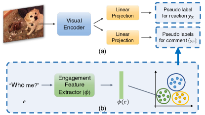
Figure 2: Learning from visual engagement. (a) We learn visual representations by predicting the pseudo-labels derived from a set of engagement signals including comments and raw reactions. (b) The pseudo-label is the clustered assignment index that is computed by first transforming the raw engagement ($e$) to a numerical representation $\phi(e)$. See the main text for more details.

3.1 From Engagement to Labels

How people react to images is more telling than the content itself. In this work, we propose to predict raw social engagement signals by converting them into a bag-of-word multi-label multi-task classification task. Fig. 2 illustrates the pipeline we use in this work.

More formally, let $(x,\{e\})$ be an image and a set of corresponding engagement clues (e.g., comments, replies, likes, etc.). Let $\phi$ be a general engagement feature extractor that transforms $e$ into a numerical representation $\phi(e)\in\mathds{R}^{D}$. We describe the proposed method to preprocess and obtain pseudo-label for $e$ below.

Step 1 (Cluster Generation)

We first collect $e$ from a randomly sampled subset of the entire image-engagement pairs and generate $k$ clusters using $K$-means algorithm. This portion of the dataset will not be used during pre-training.

Step 2 (Label Creation)

Given the $i^{th}$ example from the unprocessed subset, $(x_{i},\{e\}_{i})$, we obtain a set of features $\{\phi(e)\}_{i}$ from the engagement set of this example, using the same function $\phi$. Next we collect the resulting cluster assignments indices as a set of labels $\{y_{e}\}$ for this image $x_{i}$. Fig. 2(a) summarizes this step.

3.2 Engagement Types

We use textual comments ($\mathcal{C}$) and raw reactions ($\mathcal{R}$) from publicly available Facebook posts as a first step to investigate visual engagement signals for representation learning.

Comments Comments are direct human responses from image posts. Maximal 100 comments are randomly sampled from a post. We use the bag-of-word approach with the term frequency-inverse document frequency (TF-IDF) weighted document embeddings [68] as comment feature extractor $\phi_{\mathcal{C}}$. The cluster assignments derived from the comment set are used as multi-label classification targets, one label for each sampled comment associated with this specific image.

Raw reactions Reactions are encoded as a normalized distribution over the five reaction buttons (“haha”, “sorry”, “angry”, “wow”, “love”). More specifically, we count the total occurrences of the 5 reaction buttons for each image post and normalize (L2) them to account for differences in followers and popularity of the post. Each post is mapped to a single cluster centroid index.

3.3 Training VisE Models

VisE learning objective VisE is trained in a multi-task learning framework by minimizing the following loss function:

$$\operatorname*{arg\,min}_{W}\mathbb{E}_{(x_{i},\{y_{e}\}_{i})\sim\mathcal{D}}\,\, \mathcal{L_{C}}(f(x_{i}),\{y_{\mathcal{C}}\}_{i};W)$$

$$+\, \mathcal{L_{R}}(f(x_{i}),\{y_{\mathcal{R}}\}_{i};W),$$ (1)

where $\mathcal{L_{C}}$ is a cross-entropy loss with soft probability [55], $\mathcal{L_{R}}$ is the standard cross-entropy loss, $f$ represents an image feature encoder parameterized by $W$. $\mathcal{D}$ represents the training data which the image-engagement pairs are sampled from. In addition, $\{y_{\mathcal{C}}\}$ and $\{y_{\mathcal{R}}\}$ denote the pseudo labels of comments and reactions, respectively.

Pre-training details In our experiments, we train convolutional networks for engagement prediction. For comparison with previous work, the CNN model architectures we use are: ResNet-50, ResNet-101 [28], and ResNeXt-101 $32\times 16$d [85]. VisE model with the largest backbone, ResNeXt-101 $32\times 16$d, took around 10 days to train on 32 NVIDIA V100 GPUs with 250 million images with minibatch size of 1536. Other pre-training details are included in the Appendix C.

4 Experiments

We evaluate the effectiveness of feature representations learned by VisE for a wide range of downstream tasks. In our experiment, we aim to show that image representations learned from engagement signals are beneficial for image classification that beyond the scope of conventional recognition tasks. We begin by describing our experimental setups, including a comparison of alternative representation learning methods (Sec. 4.1), implementation details (Sec. 4.2), and a summary of evaluated downstream tasks (Sec. 4.3). Finally we present results and discussion in Sec. 4.4 and Sec. 4.5.

4.1 Compared methods

	Method	Input Type	Annotation Type	Noisy Labels	Pre-trained Data	Data Size	Model
	Random Init	-	-	-	train from scratch	-
(1)	IN-Sup	images	object labels		ImageNet [11]	1.28M	CNN
	IG-940M-IN [55]	images	hashtags + labels	✓	IG [55] + ImageNet [11]	940M + 1.28M	CNN
	MoCo-v2 [7]	image pairs	-		ImageNet [11]	83.9B⋆	CNN
	VQAGrid [35]	images	object + attribute		VisualGenome [44]	103k	Faster-RCNN
(2)	VirTex [12]	images	captions		COCO-caption [8]	118k	CNN + Transformer
	ICMLM [2]	images + captions	masked token from captions		COCO-caption [8]	118k	CNN + Transformer
	CLIP [66]	images + text	-		WebImageText [66]	13.1T⋆	CNN + Transformer
	ours	images	pseudo labels	✓	VisE-1.2M	1.23M	CNN
					VisE-250M	250M

Table 1: VisE vs. alternative methods compared. The seven representation learning approaches are grouped into: (1) Uni-modal pre-training: similar to VisE, these methods use visual encoders only during pre-training; (2) Cross-modal pre-training: like VisE, these approaches learn from natural language as inputs or supervisory signals. All three architectures involve a Transformer-based model [79] for the textual module. ^⋆We include the negative image-image / image-text pairs when counting the total data size for MoCo-v2 and CLIP. See Appendices for more details. We also acknowledge that the effective data size is also affected by other factors such as data augmentations in other approaches. For simplicity, we use the actual dataset size for non-contrastive learning methods.

To train VisE, we collect a total of 270 million public image posts from a social media platform with 20 million used for cluster generation (see Sec. 3.1). To facilitate a fair comparisons with the ImageNet-supervised method, we also randomly sample 1.23 million images for pre-training. We compare VisE pre-trained on 1.23 million (VisE-1.2M) and 250 million data (VisE-250M) with other feature representation learning methods.

Uni-modal learning methods We first compare VisE trained with pseudo labels derived from clustering assignments with networks that are trained with a pre-defined set of object labels:

• ImageNet-supervised (IN-Sup): the image encoder is pre-trained on ILSVRC 2012 [11] train split (1.28M images). The dataset has 1000 classes, which is based on the concepts in WordNet [56].

• IG-imagenet (IG-940M-IN) [55]: the visual encoder is pre-trained on 940 million public images with 1.5K hashtags in weakly-supervised fashion; the encoder is further fine-tuned on ImageNet dataset.

• VQAGrid [35]: a pre-training method primarily for visual question answering and image captioning tasks. It learns visual representations by training a Faster-RCNN [67] on the Visual Genome dataset [44] which has 1600 object categories and 400 attributes. We use the outputs from the last bottleneck block of the ResNet-50 as the pre-trained image representations.

• MoCo-v2 [27]: a self-supervised contrastive method using a momentum-based encoder and a memory queue trained on ImageNet. Given an image sample, it is trained to be closer to its randomly augmented version on a hypersphere than other samples in the dataset. We use the improved version [7] that is trained with 800 epochs. Note that this method uses image as supervision labels instead of the ImageNet class labels.

Cross-modality pre-training Learning methods that use natural language as supervisory signals are also considered:

• ICMLM [2]: it uses 118K image-text pairs from COCO-captions [8] and uses masked language modeling to learn visual representations from text. We include two versions of this method, ICMLM_tfm and ICMLM_att-fc, which respectively use a transformer and an attention-based mechanism for joint fine-tuning.

• VirTex [12]: this method also pre-trains on COCO-captions but on a different task: generating captions based on images.

• CLIP [66]: Contrastive Language-Image Pre-training method (CLIP) utilizes an image encoder and a text encoder to predict which images are paired with which textual descriptions in a large-scale dataset of 400M image-text pairs.

It is worth pointing out all of these approaches train a text encoder to learn better natural language representations during pre-training stage, while VisE simply uses an off-the-shelf text encoder to compute representations for clustering purposes. We expect better performance of VisE if these textual representations are further fine-tuned [3] as these aforementioned methods.

We also report results of “Random Init”, where no pre-trained features are used. Table 1 summarizes the differences between VisE and all of the baseline methods used in the experiment.

4.2 Evaluation Protocols and Details

We adopt two common protocols for evaluating the effectiveness of feature representations [55, 21, 57, 27]: (1) Linear evaluation: all pre-trained models are used as visual feature extractors, where the weights of the image encoders are fixed. This protocol is preferred for applications where computational resources or training data for target tasks are limited. The test performance indicates how effective the learned representations are for specific tasks. (2) Fine-tuning: the parameters of the pre-trained image encoders are used as an advanced weight initialization method; these encoders are fine-tuned in an end-to-end manner for downstream tasks. Prior studies [18, 67] have shown that the latter protocol outperforms the linear evaluation approach due to its flexibility and adaptability to a wider range of downstream tasks.

See the Appendix C for more implementation details, including a full list of hyperparameters used (batch sizes, learning rates, decay schedules, etc.) and sensitivity to hyperparameters for both linear and fine-tuned experiments.

4.3 Downstream Tasks

We evaluate these visual representation methods on four downstream tasks, including sentiment classification, political bias, hate speech detection and fine-grained bird species classification.

UnbiasedEmotion Dataset This dataset [62] contains 3045 images annotated into six emotional categories. To reduce object biases in the dataset, different emotion labels contain the same set of objects/scenes. Since there is no official split of this dataset, we random split the images into train (70%), val (10%), test (20%) set five times and report mean and standard deviation of the resulting accuracy.

Politics The task of this dataset [75] is to predict the political leaning (left and right) of images from news media. This dataset contains 749,932 images in total. Since only train and testset are publicly available, we randomly split the training set into train (90%) and val (10%) and report accuracy scores.

Hateful Memes Hateful Memes dataset [40] contains multimodal memes including images and text. The task is to detect each meme is hate speech or not. We use the data from Phase 1 of the Hateful Memes challenge, which has 8500 training and 500 validation data. We obtain the sentence embeddings from a pre-trained RoBERTa model [52], and concatenate the text features and image features together before linear evaluation that map the feature to the label space. We report the macro averaged ROC AUC score and accuracy score on the val set.

Caltech-UCSD Birds-200-2011 (CUB-200-2011) In addition to the above subjective classification tasks, we also evaluate our approach on standard image classification tasks. To this end, we use the CUB-200-2011 dataset. CUB-200-2011 [80] has a total of 11,788 images allocated over 200 (mostly North American) bird species. It is a benchmarking dataset for subordinate categorization. We train on the publicly available train set and report top-1 accuracy on the val set.

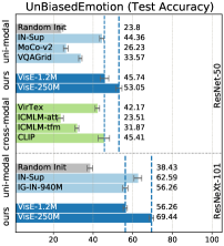
(a) Linear evaluation: UnbiasedEmotion.

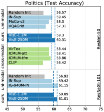
(b) Linear evaluation: Politics.

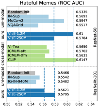
(c) Linear evaluation: Hateful Memes.

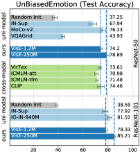
(d) Fine-tuned: UnbiasedEmotion.

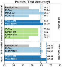
(e) Fine-tuned: Politics.

(f) Fine-tuned: Hateful Memes.

Figure 3: Linear evaluation (top) and fine-tuned (bottom) results among VisE, uni-modal (ResNet-50), cross-modal (ResNet-50), and uni-modal (ResNeXt-101 32 $\times$ 16d) methods for all three datasets. For easy comparison, two blue dashed lines represent the performance of VisE-1.2M and VisE-250M respectively.

4.4 VisE for Subjective Recognition Tasks

Following the two protocols described in Sec. 4.2, we compare the transfer-learning capabilities of VisE with other baseline approaches for three subjective tasks. Fig. 3 presents the results for the linear evaluation and fine-tuned protocols, respectively.

VisE vs. other uni-modal methods

From Fig. 3, we can see that: (1) VisE is consistently better than other image-encoder only methods on three datasets over two visual backbone choices, except for MoCo-v2 in Politics. Even pre-trained with similar amounts of data (1.28M vs. 1.23M), VisE-1.2M still achieves better performance across all three tasks with a ResNet-50 backbone than models trained with labels from In-Sup. (2) VisE-250M substantially outperforms IG-940M-IN, a method trained with a substantially larger amount of pre-trained data (950M vs. 250M). (3) MoCo-v2, a self-supervised approach that does not require object category annotations, yields the best accuracy scores on Politics among approaches with ResNet-50 backbone. This also highlights the limitation of using object labels as pre-training supervision for such subjective tasks.

VisE vs. other methods that learn from language Under both protocols, VisE offers better or comparable results than other methods that leverage textual information during pre-training. VisE achieves consistently better performance across all three tasks. This suggests that features learned with visual engagement signals are more suitable for subjective downstream tasks. We also observe that all other four visual-language approaches obtain better results than IN-Sup on UnbiasedEmotion dataset when fine-tuned, but they are worse than IN-Sup with linear evaluation. Such discrepancy might be caused by the scale of the dataset, since UnbiasedEmotion is the smallest among the other tasks.

4.5 VisE for Standard Recognition Tasks

We compare the effectiveness of features learned from visual engagement signals with those trained using ImageNet labels on CUB-200-2011. This task extends the general object classification from ImageNet and focuses on distinguishing fine-grained differences among 200 bird species. Moreover, 59 out of 1000 classes in ImageNet are already bird categories, including overlapping definitions with CUB-200-2011 [77]. Thus Image-Net based approaches should transfer to this task better than VisE. Table 2 shows the results of both linear evaluation and fine-tuned transfer protocols.

Indeed, IN-Sup and IG-940M-IN achieve decent accuracy scores using linear classifiers alone to map the features to 200 bird species, outperforming VisE by a large margin. This is foreseeable since visual engagement signals do not necessarily contain object information. It is understandable that VisE features are not as transferable to this task as models trained on ImageNet.

When fine-tuning is performed, VisE with ResNet-50 have comparable or better performance than IN-Sup. This highlights that fine-tuning the whole network can sometimes compensate for the inflexibility of learned features, which is in line with discussions in [66].

Backbone	Method	Linear	Fine-tuned
ResNet-50	Random Init	3.42	63.39
	IN-Sup	62.70	72.15
	VisE-1.2M	9.95	72.65
	VisE-250M	9.92	76.58
ResNeXt-101 $32\times 16$d	Random Init	7.04	62.80
	IN-Sup	65.16	84.21
	IG-940M-IN [55]	72.69	85.28
	VisE-1.2M	9.76	73.73
	VisE-250M	10.93	79.54

Table 2: Validation accuracy on CUB-200-2011. Features learnt from Image-Net class labels transfer well to CUB-200-2011.

5 Analysis

To better understand the values of visual engagement signals and our pre-trained VisE models, we conduct ablation studies and qualitative analysis using the same set of subjective target tasks. All experiments use the fine-tuned protocol unless otherwise specified. Additional results and analysis are included in the Appendix B).

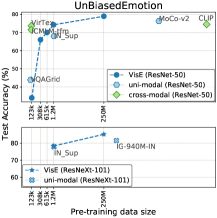
(a) UnbiasedEmotion.

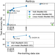
(b) Politics.

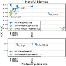
(c) Hateful Memes.

Figure 4: Data size ablation using ResNet-50 (top) and ResNeXt-101 32$\times$16d (bottom) backbones. We only present one of ICMLM_att-fc and ICMLM_tfm due to space constraint. The differences between both ICMLM methods are within 1$\%$ with each other.

Backbone	Method	UnbiasedEmotion		Politics		Hateful Memes
		Linear	Fine-tuned	Linear	Fine-tuned	Linear	Fine-tuned
ResNet-50	Reaction + Comments	45.74 $\pm$ 2.15	74.20 $\pm$ 1.93	0.6100	0.6044	64.30	64.69
	Comments	49.15 $\pm$ 1.30   $\uparrow$3.41	72.16 $\pm$ 1.09 $\downarrow$2.04	0.6005 $\downarrow$0.0095	0.5921 $\downarrow$-0.0124	63.43 $\downarrow$0.87	63.81 $\downarrow$0.88
	Reaction	33.05 $\pm$ 1.75 $\downarrow$12.69	70.03 $\pm$ 2.64 $\downarrow$4.17	0.6052 $\downarrow$0.0048	0.5980 $\downarrow$0.0064	63.09 $\downarrow$1.21	63.42 $\downarrow$1.27

Table 3: Task ablation of VisE-1.2M with ResNet-50. Colored text with $\uparrow$ and $\downarrow$ indicate the differences with results from the VisE model trained with both reaction and comments.

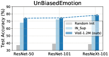
(a) UnbiasedEmotion.

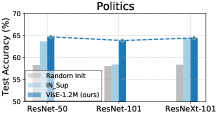
(b) Politics.

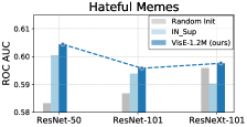
(c) Hateful Memes.

Figure 5: Visual backbone ablations.

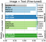
(a) Image + Text (Fine-tuned)

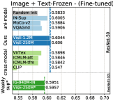
(b) Image + Text-Frozen (Fine-tuned)

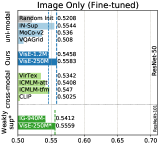
(c) Image Only (Fine-tuned)

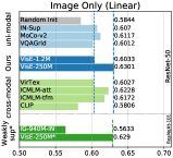
(d) Image Only (Linear)

Figure 6: Multi-modal ablation for Hateful Memes val split. For reference, using text encoder alone give ROC AUC scores: 0.6363 (fine-tuned), 0.5983 (linear).

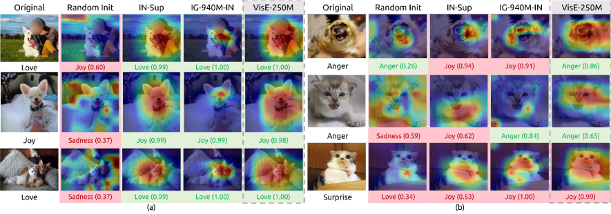
Figure 7: Qualitative results on UnbiasedEmotion dataset using ResNeXt-101 32$\times$16d.

5.1 Pre-training ablation

Effect of pre-training data size

We additionally train VisE models using randomly sampled $\{$123k, 308k, 615k$\}$ images using fine-tuned setting. Fig. 4 presents the results for three datasets compared with other baselines for easy reference. From Fig. 4(a) and 4(b), we can see that there is a positive correlation between training data size and model performance for VisE. VirTex and ICMLM achieve similar results as VisE with less training data (118k vs. $\{$615k, 1.23M$\}$). This shows the noisy pseudo-labels from visual engagement might need more data to compensate its weakly-supervised nature.

For a multi-modal dataset like Hateful Memes, the correlation between data size and performance is less clear than the other two tasks, as shown in Fig. 4(c). When fine-tuned, VisE is able to perform better than other baselines, demonstrating the effectiveness of visual engagement signals.

Effect of pre-training tasks

VisE is trained using cluster assignments from both comments and raw reactions. Table 3 shows the ablation study where we evaluate the contribution of different engagement formats. In general, VisE obtains the best performance when trained with a multi-task objective.

Effect of pre-training visual backbone  Fig. 5 presents ablation studies using different visual backbones. VisE-1.2M is better than Random Init and IN-Sup across all three backbone choices and three downstream tasks. We also note that the advantages of VisE is diminishing as the number of parameters of backbone getting larger possibly due to overfitting on the downstream training set.

5.2 Multimodal fine-tuning ablation

We used an image encoder and a frozen textual encoder for experiments on Hateful Memes dataset in Sec 4. To isolate the effects of both module for this dataset, we compare VisE with other baselines under the following setups: (1) Image + Text (Fine-tuned): parameters from both encoders are updated during transfer learning. (2) Image + Text-Frozen (Fine-tuned): the same fine-tuned setting as the experiment in Sec 4. (3) Image Only (Fine-tuned): we only use image encoder in fine-tuned setting. (4) Image Only (Linear): image encoder is used as feature extractor only. Note the linear evaluation of Hateful Memes in Sec. 4.4 (Fig. 3(c)) uses concatenated features from both encoders. Fig. 6 presents the results.

Methods with VisE are able to achieve better or comparable results compared with other baselines. And visual-language methods outperform IN-Sup in Fig. 6(a) except for CLIP. This shows the visual backbones that are pre-trained with a textual module are better when both modules are fine-tuned together.

From Figs. 6(a)-6(c), the ROC AUC scores are getting smaller and smaller as the textual encoder makes less and less contribution. This demonstrates that the text module has dominant effect on predicting if a multi-modal meme is hateful or not. If using image encoders only, linear evaluation obtains better results than the fine-tuned protocol (Fig. 6(c) vs. 6(d)). This also suggests textual information is more important on this dataset.

5.3 Qualitative Analysis

We also conduct qualitative studies using UnbiasedEmotion to further understand the benefit of visual engagement. Fig. 7 shows sample predictions produced by our VisE-250M and 3 other approaches. The predicted classes for each approach are color coded (green as correct, red as incorrect). We also use class activation mappings [94] to visualize the discriminate image regions for the predicted emotion. Although all methods that are initialized with pre-trained models can detect the object of interest in the image, IN-Sup and IG-940M-IN are more likely to predict “joy” and “love” for the cats and dogs photos in Fig. 7, while VisE-250M yields more diverse predictions (see row 2 left vs. row1 right as an example). This seems to suggest that IN-Sup and IG-940M-IN map dogs and cat to positive emotions. VisE-250M, on the other hand, does not rely on the ImageNet object labels during pre-training and is able to distinguish the subtle emotional differences among different images with dogs and cats. However, all methods failed to infer “surprise” from the bottom left image, possibly due to imbalanced training data of UnbiasedEmotion. Additional visualization can be found in the Appendix A.

6 Conclusion

We explored social media visual engagement as supervisory signals for representation learning. We presented VisE, a streamlined pre-training method that uses pseudo-labels derived from human responses to social media posts, including reactions and comments. Experiments and analysis show that visual engagement signals transfer well to various downstream tasks that go beyond conventional visual recognition. VisE is able to outperform various representation learning models on these datasets. We therefore hope that VisE could inspire and facilitate future research that focuses on the cognitive aspects of images. Pre-trained models will be released upon acceptance of the work.

Acknowledgement We thank Marseille who is featured in Figs. 1 and 2. This work is supported by a Facebook AI research grant awarded to Cornell University.

Appendix A Qualitative Analysis

Fig. 8 presents more predicted examples including images with dogs and parks. It further shows that ImageNet based pre-training methods tend to map certain objects to a certain set of emotions. VisE, on the other hand, is able to predict correct emotions in these examples.

Appendix B Supplementary Results and Discussion

Transfer learning on ImageNet

Table 4 presents results and comparisons on ImageNet. We fine-tune VisE-250M with a ResNeXt-101 backbone on ImageNet, and compare the val accuracy scores with the same ResNeXt-101 model trained from scratch (IN-Sup). We also show the results of IG-940M-IN [55], which is pre-trained on 940 million images with 1.5K hashtags and fine-tuned on ImageNet using the same visual backbone. We see from Table 4 that representations learned from VisE-250M with engagement signals are transferable to ImageNet, outperforming the IN-Sup model by 0.88 (1.12%) measured by Top-1 accuracy. Note that engagement signals are relatively weak compared to the hashtags used in IG-940M-IN, which were selected to match with 1000 ImageNet synsets. Our goal here is to show features learned by VisE can be generalized to large-scale image classification tasks.

Images vs. engagement signals

To disentangle the effect of training images and engagement signals, we also trained MoCo-v2 with the same 1.23 million social post data (VisE-1.2M(MoCo-v2)). Table 5 shows the linear evaluation results on UnbiasedEmotion, which shows the engagement signals, not the images, are beneficial for this dataset. We will include the full results in the final version.

Additional results

Table 6 and 7 present full transfer learning results including performance on the val split and an additional metric for the Hateful Memes dataset. These two tables can be read in conjunction with the main figure and the backbone ablation studies in the main text. Note that we use in-house baselines instead of copying results from prior work for fair-comparison purposes. All the experiments are trained using the same grid search range, validation set, learning rate schedule, etc. We use validation accuracy and ROC AUC for Hateful Memes to select the best set of hyper-parameters. See Appendix C.3 for details.

Datasize calculation for contrastive learning methods

In size ablation studies, we sort all pre-training methods by the training inputs size. We consider the negative input pairs for MoCo-v2 and CLIP as the effective training data size.

• MoCo-v2 uses image pairs from ImageNet as inputs. The total class size is the total number of training data (1.28 million). The effective training data size is the number of image pairs used, which is (k + 1) $\times$ 1.28M = 83.9B, where $k=65536$ is the number of images in the queue for MoCo-v2.

• CLIP uses a dataset with 400M image-text pairs. This approach considers the pair-wise similarity among image-text in a batch during training. Since the batch size is 32768, the total effective datasize is $400$M $/32768\times 32768\times 32768=83.9$B.

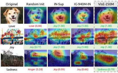
Figure 8: Qualitative results on UnbiasedEmotion dataset using ResNeXt-101 32$\times$16d backbone.

Method	Top 1 Accuracy	Top 5 Accuracy
IN-Sup	78.78	94.12
VisE-250M	79.66 $\uparrow$0.88	94.62 $\uparrow$0.5
IG-940M-IN [55]	84.2	97.2

Table 4: Fine-tuned experiments on ImageNet with ResNeXt-101 32 $\times$ 16d backbone. Colored text with $\uparrow$ indicate the differences between VisE and IN-Sup.

Method	Val Accuracy	Test Accuracy
VisE-1.2M (MoCo-v2)	27.96 $\pm$ 2.91	27.80 $\pm$ 2.30
VisE-1.2M	44.67 $\pm$ 3.52 $\uparrow$16.71	45.74 $\pm$ 2.15 $\uparrow$17.94

Table 5: Linear evaluation experiments on UnbiasedEmotion with ResNet-50 using the same 1.23 million data.

Backbone	Method	UnbiasedEmotion		Politics		Hateful Memes
		Val Accuracy	Test Accuracy	Val Accuracy	Test Accuracy	ROC AUC	Accuracy
ResNet-50	Random Init	24.67 $\pm$ 2.78	23.80 $\pm$ 1.02	56.80	56.57	0.5335	51.64
	Uni-modality pre-training methods
	IN-Sup	43.62 $\pm$ 2.31	44.36 $\pm$ 1.09	59.31	59.45	0.5691	53.16
	VQAGrid [35]	32.17 $\pm$ 1.22	33.57 $\pm$ 0.86	57.32	57.31	0.5517	53.2 $\uparrow$0.04
	Cross-modalities pre-training methods
	VirTex [12]	40.59 $\pm$ 2.96	42.17 $\pm$ 1.14	58.46	58.44	0.5659	54.40 $\uparrow$1.24
	ICMLMatt-fc [2]	23.81 $\pm$ 2.25	23.51 $\pm$ 1.52	58.27	58.41	0.5702 $\uparrow$0.0011	53.32 $\uparrow$0.16
	ICMLMtfm [2]	31.71 $\pm$ 2.02	31.87 $\pm$ 0.95	58.73	58.86	0.5631	53.24 $\uparrow$0.08
	Contrastive learning pre-training methods
	MoCo-v2 [7]	26.31 $\pm$ 1.12	26.23 $\pm$ 1.20	58.14	58.30	0.5947 $\uparrow$0.0256	53.92 $\uparrow$0.76
	CLIP [66]	42.70 $\pm$ 3.02	45.41 $\pm$ 2.90 $\uparrow$1.05	56.65	56.42	0.6147 $\uparrow$0.0456	57.04 $\uparrow$3.88
	Ours
	VisE-1.2M	44.67 $\pm$ 3.52 $\uparrow$1.05	45.74 $\pm$ 2.15 $\uparrow$1.38	59.15 $\downarrow$0.16	59.30 $\downarrow$0.15	0.6100 $\uparrow$0.0409	55.52 $\uparrow$2.36
	VisE-250M	51.97 $\pm$ 4.08 $\uparrow$8.35	53.05 $\pm$ 1.48 $\uparrow$8.69	60.56 $\uparrow$1.25	60.31 $\uparrow$0.86	0.5784 $\uparrow$0.0093	54.48 $\uparrow$1.32
ResNeXt-101 $32\times 16$d	Random Init	37.96 $\pm$ 3.77	38.43 $\pm$ 1.38	57.05	56.92	0.5466	53.64
	IN-Sup	63.09 $\pm$ 3.12	62.59 $\pm$ 1.99	59.24	59.42	0.5542	51.84
	IG-940M-IN [55]	55.86 $\pm$ 1.36	56.26 $\pm$ 1.32	60.98 $\uparrow$1.74	61.15 $\uparrow$1.73	0.5482	52.28 $\uparrow$0.44
	VisE-1.2M (ours)	56.64 $\pm$ 2.49 $\downarrow$6.45	56.26 $\pm$ 1.05 $\downarrow$6.33	59.70 $\uparrow$0.46	59.89 $\uparrow$0.47	0.5621 $\uparrow$0.0079	54.24 $\uparrow$2.40
	VisE-250M (ours)	69.61 $\pm$ 2.74 $\uparrow$6.51	69.44 $\pm$ 1.20 $\uparrow$6.85	61.08 $\uparrow$1.84	61.01 $\uparrow$1.59	0.5795 $\uparrow$0.0253	56.04 $\uparrow$4.20

Table 6: Linear evaluation experiments comparing VisE with other pre-training baselines. Colored text with $\uparrow$ and $\downarrow$ indicate the differences between VisE and IN-Sup with the same visual backbone. $\uparrow$ is also used if other methods yield better results than IN-Sup. In general, VisE outperforms the ImageNet supervised and hashtag-based weakly supervised pre-training methods.

Backbone	Method	UnbiasedEmotion		Politics		Hateful Memes
		Val Accuracy	Test Accuracy	Val Accuracy	Test Accuracy	ROC AUC	Accuracy
ResNet-50	Random Init	39.01 $\pm$ 0.99	37.25 $\pm$ 2.12	58.28	58.31	0.5833	51.84
	Uni-modality pre-training methods
	IN-Sup	69.87 $\pm$ 3.27	67.94 $\pm$ 3.18	63.87	63.64	0.6005	54.32
	VQAGrid [35]	42.17 $\pm$ 3.07	43.93 $\pm$ 1.56	58.31	58.1	0.5906	53.24
	Cross-modalities pre-training methods
	VirTex [12]	72.24 $\pm$ 2.13 $\uparrow$2.37	73.61 $\pm$ 1.94 $\uparrow$5.67	63.24	63.06	0.5898	53.84
	ICMLMatt-fc [2]	71.65 $\pm$ 2.31 $\uparrow$1.78	70.98 $\pm$ 2.01 $\uparrow$3.05	63.3	63.2	0.5846	53.52
	ICMLMtfm [2]	70.92 $\pm$ 1.65 $\uparrow$1.05	71.48 $\pm$ 1.78 $\uparrow$3.54	63.43	63.21	0.5842	53.40
	Contrastive learning pre-training methods
	MoCo-v2 [7]	77.63 $\pm$ 1.78 $\uparrow$7.76	76.23 $\pm$ 1.88 $\uparrow$8.29	66.24 $\uparrow$2.37	66.37 $\uparrow$2.73	0.5884	52.48
	CLIP [66]	73.68 $\pm$ 0.93 $\uparrow$3.81	74.46 $\pm$ 1.21 $\uparrow$6.53	58.08	58.07	0.5470	53.48
	Ours
	VisE-1.2M	73.82 $\pm$ 1.07 $\uparrow$3.95	74.20 $\pm$ 1.93 $\uparrow$6.26	64.69 $\uparrow$0.82	64.69 $\uparrow$1.05	0.6070 $\uparrow$0.0039	55.88 $\uparrow$0.96
	VisE-250M	79.74 $\pm$ 1.54 $\uparrow$9.87	78.89 $\pm$ 2.23 $\uparrow$10.95	65.83 $\uparrow$1.96	65.62 $\uparrow$1.98	0.6060 $\uparrow$0.0055	55.00 $\uparrow$0.68
ResNet-101	Random Init	40.20 $\pm$ 2.76	39.08 $\pm$ 1.72	58.18	58.07	0.5868	53.48
	IN-Sup	71.84 $\pm$ 2.72	72.43 $\pm$ 2.24	58.28	58.42	0.5939	54
	VisE-1.2M (ours)	73.82 $\pm$ 0.77 $\uparrow$1.97	74.52 $\pm$ 1.18 $\uparrow$2.10	63.92 $\uparrow$5.64	63.85 $\uparrow$5.43	0.5958 $\uparrow$0.0019	52.96 $\downarrow$1.04
ResNeXt-101 $32\times 16$d	Random Init	40.20 $\pm$ 2.65	38.59 $\pm$ 0.91	58.26	58.39	0.5959	54.68
	IN-Sup	79.00 $\pm$ 2.33	77.92 $\pm$ 2.38	64.22	64.25	0.5903	52.92
	IG-940M-IN [55]	83.24 $\pm$ 1.68 $\uparrow$4.24	81.52 $\pm$ 1.76 $\uparrow$3.60	65.90 $\uparrow$1.68	65.58 $\uparrow$1.33	0.5951 $\uparrow$0.0048	54.28 $\uparrow$1.36
	VisE-1.2M (ours)	77.57 $\pm$ 2.43 $\downarrow$1.43	78.33 $\pm$ 1.39 $\uparrow$0.41	64.61 $\uparrow$0.39	64.44 $\uparrow$0.19	0.5976 $\uparrow$0.0073	54.40 $\uparrow$1.48
	VisE-250M (ours)	84.08 $\pm$ 1.87 $\uparrow$5.08	85.21 $\pm$ 1.24 $\uparrow$7.29	67.61 $\uparrow$3.39	67.64 $\uparrow$3.39	0.5957 $\uparrow$0.0054	54.96 $\uparrow$2.04

Table 7: Fine-tuning experiment comparing VisE with other pre-training baselines. Colored text with $\uparrow$ and $\downarrow$ indicate the differences with IN-Sup with the same visual backbone. $\uparrow$ is also used if other methods yield better results than IN-Sup. Similar to observations in Table 6, VisE can achieve better results compared to the ImageNet supervised and hashtag-based weakly supervised pre-training methods.

Appendix C Reproducibility Details

C.1 VisE Pre-training Setup

Optimization

VisE models are trained on 32 GPUs across 4 machines with a batch size of 1920 images for the ResNet backbone and 1536 for the ResNeXt backbone. We use stochastic gradient descent with a momentum of 0.9 and a weight decay of 0.0001. The base learning rate is set according to $0.1/256\times b$, where $b$ is the batch size used for the particular model. The learning rate is warmed up linearly from 0 to the base learning rate during the first $5\%$ of the whole iterations. The learning rate decay schedule is set differently for VisE-1.2M and VisE-250M. For models that use 1.23 million images, we follow common ImageNet pre-training settings. For models that are trained with 250 million images, the learning rate is reduced 10 times over approximately 10 epochs with the scaling factor of 0.5.

Training details

We adopt standard image augmentation strategy during training (randomly resize crop to 224 $\times$ 224 and random horizontal flip). Since the dataset is not balanced, we follow [50, 10] to stabilize the training processing by initializing the the bias for the last linear classification layer with $b=-\log\left(\left(1-\pi\right)/\pi\right)$, where the prior probability $\pi$ is set to 0.01. To obtain the pseudo-labels for the visual engagement signals, we set the number of clusters as 5000 and 128, for comments and raw reactions respectively.

Other details

We spend around 9 hours to mine the data for pretraining with 3 server nodes (144 cpus). For the 1.23M data, the total word count for comments is 178M, the average _{$\pm$ std} number of comments per image is 20.25 _{$\pm$ 54.43} , the average _{$\pm$ std} reactions count per image is 81.21 _{$\pm$ 601.4} . We use Pytorch [63] to implement and train all the models on NVIDIA Tesla V100 GPUs.

Dataset	Task	# Classes	Train	Val	Test
Caltech-UCSD Birds-200-2011 [80]	Fine-grained bird species recognition	200	5994	5794	-
UnbiasedEmotion [62]	Image emotion recognition	6	2,131⋆	304⋆	610⋆
Politics [75]	Visual political bias prediction	2	607,306⋆	67,478⋆	75,148
Hateful Memes [40]	Hate speech detection in multimodal memes	2	8,500	500	-

Table 8: Specifications of the various target task dataset. Image number with ^⋆ are the subset we randomly sampled since no publicly data splits are available. UnbiasedEmotion are randomly split 5 times.

Task	# GPUs	ResNet-50 (24M)		ResNet-101 (45M)		ResNeXt-101 (194M)
		Per Iteration (second)	Total Time (minute)	Per Iteration (second)	Total Time (minute)	Per Iteration (second)	Total Time (minute)
UnbiasedEmotion	1	1.67	49.64	1.44	50.30	1.32	63.37
Politics	8	0.14	216.26	0.18	243.64	0.67	721.61
Hateful Memes	1	0.43	41.23	0.32	49.57	0.50	140.81
CUB-200-2011	1	0.74	294.01	-	-	0.91	1,304.01

Table 9: Average run time (per iteration and total) for fine-tuned experiments.

Training Schedule

Method

Batch Size

Linear Evaluation

Fine-tuned

Base LR

WD

$S_{lr}$

$S_{wd}$

Base LR

WD

$S_{lr}$

$S_{wd}$

UnbiasedEmotion

Total epochs: 50 LR steps: (0, 10, 20, 30) LR decay: (1, 0.1, 0.01, 0.001)

ResNet-50

Random Init

128

0.025

{0.001, 0.01, 0.0001, 0.01, 0.01}

1.28 $\pm$ 0.38

0.36 $\pm$ 0.06

{0.0025, 0.025, 0.025, 0.0025, 0.0025 }

{0.0001, 0.001, 0.01, 0.01, 0.01}

4.39 $\pm$ 0.75

1.54 $\pm$ 0.54

IN-Sup

0.025

{0.01, 0.0001, 0.01, 0.01, 0.01}

10.52 $\pm$ 0.65

0.38 $\pm$ 0.26

{0.0025, 0.0025, 0.0025, 0.0025, 0.025 }

{0.0001, 0.001, 0.001, 0.01, 0.0001}

7.35 $\pm$ 1.18

2.10 $\pm$ 0.50

MoCo-v2

0.025

{0.01, 0.01, 0.0001, 0.01, 0.01}

3.06 $\pm$ 0.33

0.47 $\pm$ 0.18

0.0025

{0.0001, 0.01, 0.0001, 0.001, 0.0001}

3.94 $\pm$ 0.47

0.42 $\pm$ 0.28

VQAGrid

0.025

{0.0001, 0.0001, 0.0001, 0.01, 0.01}

6.91 $\pm$ 0.57

0.51 $\pm$ 0.21

0.00025

{0.0001, 0.0001, 0.0001, 0.01, 0.01}

0.00 $\pm$ 0.00

0.64 $\pm$ 0.39

VirTex

0.025

{0.001, 0.0001, 0.01, 0.0001, 0.01}

7.70 $\pm$ 0.45

0.41 $\pm$ 0.39

0.0025

{0.01, 0.0001, 0.001, 0.001, 0.001}

3.76 $\pm$ 0.64

0.81 $\pm$ 0.25

ICMLMatt-fc

0.025

{0.001, 0.001, 0.01, 0.01, 0.0001}

2.20 $\pm$ 0.81

0.21 $\pm$ 0.07

0.025

{0.01, 0.0001, 0.0001, 0.001, 0.0001}

12.38 $\pm$ 1.33

0.76 $\pm$ 0.40

ICMLMtfm

0.025

{0.01, 0.01, 0.01, 0.01, 0.01}

6.08 $\pm$ 1.17

0.83 $\pm$ 0.35

0.025

{0.01, 0.0001, 0.01, 0.01, 0.0001}

6.81 $\pm$ 0.44

1.03 $\pm$ 0.46

CLIP

0.025

{0.01, 0.01, 0.01, 0.01, 0.01}

9.88 $\pm$ 0.78

0.84 $\pm$ 0.29

2.5e-05

{0.01, 0.0001, 0.01, 0.0001, 0.001}

19.42 $\pm$ 0.79

4.36 $\pm$ 4.34

VisE-1.2M

0.025

{0.001, 0.01, 0.01, 0.01, 0.01}

10.04 $\pm$ 0.75

0.81 $\pm$ 0.52

0.025

{0.01, 0.0001, 0.001, 0.001, 0.001}

3.36 $\pm$ 0.87

1.84 $\pm$ 0.83

VisE-250M

0.025

0.01

14.35 $\pm$ 2.10

1.07 $\pm$ 0.24

0.0025

{0.001, 0.001, 0.001, 0.001, 0.01}

11.24 $\pm$ 2.84

1.77 $\pm$ 0.31

VisE-123$k$

128

-

-

-

-

0.025

{0.01, 0.0001, 0.001, 0.001, 0.0001}

3.62 $\pm$ 0.84

0.68 $\pm$ 0.39

VisE-308$k$

-

-

-

-

0.025

{0.001, 0.001, 0.001, 0.01, 0.0001}

3.21 $\pm$ 0.87

1.07 $\pm$ 0.63

VisE-615$k$

-

-

-

-

{0.0025, 0.0025, 0.025, 0.025, 0.025}

{0.0001, 0.0001, 0.0001, 0.001, 0.01}

2.98 $\pm$ 0.97

1.08 $\pm$ 0.64

VisE-1.2M-$\mathcal{C}$

-

-

-

-

{0.0025, 0.0025, 0.0025, 0.025, 0.025 }

{0.001, 0.0001, 0.0001, 0.001, 0.01}

3.00 $\pm$ 0.72

1.09 $\pm$ 0.79

VisE-$\mathcal{R}$

-

-

-

-

{0.025, 0.0025, 0.025, 0.0025, 0.025 }

{0.001, 0.001, 0.001, 0.01, 0.01}

2.18 $\pm$ 0.63

0.94 $\pm$ 0.78

ResNet-101

Random Init

64

-

-

-

-

{0.0025, 0.00025, 0.00025, 0.00025, 0.00025}

{0.01, 0.0001, 0.001, 0.0001, 0.0001}

5.79 $\pm$ 0.67

2.00 $\pm$ 1.08

IN-Sup

-

-

-

-

0.0025

{0.01, 0.0001, 0.001, 0.01, 0.0001}

7.76 $\pm$ 2.69

1.23 $\pm$ 0.51

VisE-1.2M

-

-

-

-

0.025

{0.01, 0.0001, 0.0001, 0.0001, 0.0001}

3.16 $\pm$ 0.74

1.04 $\pm$ 0.38

ResNeXt-101

Random Init

32

0.025

0.0001

2.33 $\pm$ 1.12

0.30 $\pm$ 0.13

0.025

{0.001, 0.0001, 0.01, 0.001, 0.001}

2.74 $\pm$ 0.88

0.93 $\pm$ 0.36

IN-Sup

0.025

{0.0001, 0.0001, 0.0001, 0.01, 0.0001}

9.92 $\pm$ 1.04

0.12 $\pm$ 0.12

0.025

{0.01, 0.0001, 0.001, 0.01, 0.001}

12.79 $\pm$ 1.48

1.37 $\pm$ 0.70

IG-940M-IN

0.025

{0.0001, 0.0001, 0.01, 0.0001, 0.0001}

10.15 $\pm$ 1.42

0.19 $\pm$ 0.12

0.025

{0.001, 0.0001, 0.001, 0.001, 0.001}

15.21 $\pm$ 5.96

1.25 $\pm$ 0.43

VisE-1.2M

0.025

{0.01, 0.001, 0.01, 0.01, 0.01}

13.86 $\pm$ 0.80

0.32 $\pm$ 0.20

0.0025

{0.0001, 0.001, 0.0001, 0.01, 0.001}

19.07 $\pm$ 8.31

1.60 $\pm$ 0.29

VisE-250M

0.025

{0.0001, 0.01, 0.0001, 0.0001, 0.0001}

11.29 $\pm$ 0.79

0.12 $\pm$ 0.15

0.0025

{0.01, 0.001, 0.0001, 0.01, 0.0001}

13.73 $\pm$ 0.95

0.31 $\pm$ 0.22

Table 10: Hyperparameter configurations for best-performing UnbiasedEmotion models for five random split. Single number are displayed if the configurations are the same across all five experiments.

	Training Schedule	Backbone	Method	Batch Size	Linear Evaluation				Fine-tuned
					Base LR	WD	$S_{lr}$	$S_{wd}$	Base LR	WD	$S_{lr}$	$S_{wd}$
Politics	Total epochs: 25 LR steps: (0, 10, 20) LR decay: (1, 0.1, 0.01)	ResNet-50	Random Init	192	0.0025	0.01	2.37	1.49	0.025	0.0001	0.66	0.80
			IN-Sup		0.025	0.001	2.72	0.07	0.0025	0.001	1.81	0.82
			MoCo-v2		0.025	0.0001	1.83	0.59	0.025	0.0001	0.75	3.46
			VQAGrid		0.0025	0.01	2.02	0.36	0.00025	0.001	0.00	0.43
			VirTex		0.025	0.001	2.58	0.44	0.025	0.0001	0.19	2.14
			ICMLMatt-fc		0.025	0.001	2.37	0.39	0.025	0.0001	1.06	2.05
			ICMLMtfm		0.025	0.001	2.90	0.31	0.025	0.0001	0.69	2.48
			CLIP		0.025	0.001	1.54	0.05	0.000025	0.001	0.45	0.24
			VisE-1.2M		0.025	0.001	2.60	0.27	0.025	0.0001	0.61	2.23
			VisE-250M		0.025	0.001	2.69	0.34	0.00025	0.01	3.83	0.15
			VisE-123$k$	192	-	-	-	-	0.025	0.0001	0.39	0.11
			VisE-308$k$		-	-	-	-	0.025	0.0001	1.01	2.41
			VisE-615$k$		-	-	-	-	0.025	0.0001	0.72	1.71
			VisE-1.2M-$\mathcal{C}$		-	-	-	-	0.025	0.0001	0.42	2.54
			VisE-$\mathcal{R}$		-	-	-	-	0.025	0.0001	0.36	2.17
		ResNet-101	Random Init	192	-	-	-	-	0.025	0.001	0.48	0.69
			IN-Sup		-	-	-	-	0.025	0.0001	0.61	0.77
			VisE-1.2M		-	-	-	-	0.025	0.0001	0.49	2.16
		ResNeXt-101	Random Init	192	0.0025	0.001	0.07	0.05	0.025	0.0001	0.61	0.80
			IN-Sup		0.0025	0.0001	0.08	0.06	0.025	0.0001	1.26	1.76
			IG-940M-IN		0.0025	0.001	3.36	0.01	0.0025	0.0001	2.63	1.37
			VisE-1.2M		0.025	0.0001	0.59	0.48	0.025	0.0001	0.80	2.74
			VisE-250M		0.025	0.001	0.64	0.53	0.025	0.0001	0.16	2.03

Table 11: Hyperparameter configurations for best-performing Politics models. “Batch Size” presents the total mini batch size across 8GPUs. For fine-tuned settings, some learning processes are stopped early.

	Training Schedule	Backbone	Method	Batch Size	Linear Evaluation				Fine-tuned
					Base LR	WD	$S_{lr}$	$S_{wd}$	Base LR	WD	$S_{lr}$	$S_{wd}$
Hateful Memes	Total epochs: 30 LR steps: (0, 20) LR decay: (1, 0.5)	ResNet-50	Random Init	64	0.025	0.01	0.0184	0.0022	0.025	0.01	0.0322	0.0014
			IN-Sup		0.025	0.01	0.0184	0.0006	0.025	0.0001	0.0346	0.0064
			MoCo-v2		0.025	0.01	0.0364	0.0009	0.025	0.001	0.0265	0.0022
			VQAGrid		0.025	0.01	0.0265	0.001	0.025	0.0001	0.0442	0.0426
			VirTex		0.025	0.01	0.0194	0.0018	0.025	0.001	0.0301	0.0011
			ICMLMatt-fc		0.025	0.01	0.018	0.0002	0.025	0.001	0.0353	0.0011
			ICMLMtfm		0.025	0.01	0.0217	0.002	0.025	0.01	0.0395	0.0024
			CLIP		0.025	0.01	0.0583	0.0007	0.00025	0.01	0	0.0021
			VisE-1.2M		0.025	0.01	0.0453	0.0015	0.025	0.01	0.0403	0.0061
			VisE-250M		0.025	0.01	0.0191	0.0018	0.025	0.0001	0.0284	0.0063
			VisE-123$k$	64	-	-	-	-	0.025	0.01	0.0452	0.0033
			VisE-308$k$		-	-	-	-	0.025	0.01	0.0324	0.0014
			VisE-615$k$		-	-	-	-	0.025	0.0001	0.0341	0.0074
			VisE-1.2M-$\mathcal{C}$		-	-	-	-	0.025	0.001	0.029	0.0033
			VisE-$\mathcal{R}$		-	-	-	-	0.025	0.001	0.0318	0.0043
		ResNet-101	Random Init	32	-	-	-	-	0.025	0.01	0.0404	0.0062
			IN-Sup		-	-	-	-	0.025	0.01	0.0378	0.0053
			VisE-1.2M		-	-	-	-	0.025	0.01	0.0368	0.0088
		ResNeXt-101	Random Init	16	0.00025	0.0001	0.0046	0	0.025	0.0001	0.0365	0.0015
			IN-Sup		0.025	0.01	0.02	0.0006	0.025	0.001	0.0348	0.009
			IG-940M-IN		0.025	0.01	0.0308	0.001	0.025	0.01	0.032	0.0018
			VisE-1.2M		0.025	0.01	0.0273	0.0016	0.025	0.01	0.0404	0.0021
			VisE-250M		0.025	0.01	0.0161	0.0018	0.025	0.01	0.0324	0.0051

Table 12: Hyperparameter configurations for best-performing Hateful Memes models. The text encoder is used as a feature extractor in these experiments.

	Training Schedule	Backbone	Method	Batch Size	Linear Evaluation				Fine-tuned
					Base LR	WD	$S_{lr}$	$S_{wd}$	Base LR	WD	$S_{lr}$	$S_{wd}$
CUB-200-2011	Total epochs: 300 LR steps: (0, 100, 200) LR decay: (1, 0.1, 0.01)	ResNet-50	Random Init	128	0.025	0.001	1.17	0.20	0.025	0.01	23.12	14.49
			IN-Sup		0.025	0.001	25.25	0.62	0.025	0.01	10.14	0.99
			VisE-1.2M		0.025	0.0001	4.04	0.75	0.025	0.001	10.41	1.31
			VisE-250M		0.025	0.0001	3.87	0.94	0.025	0.001	4.71	0.80
		ResNeXt-101	Random Init	32	0.025	0.0001	1.86	0.91	0.025	0.01	27.50	8.04
			IN-Sup		0.025	0.0001	8.83	0.06	0.025	0.0001	2.97	3.23
			IG-940M-IN		0.025	0.0001	23.98	0.72	0.0025	0.001	1.13	0.00
			VisE-1.2M		0.025	0.001	3.28	0.96	0.025	0.001	29.39	0.60
			VisE-250M		0.025	0.0001	3.19	1.22	0.025	0.001	30.14	2.42

Table 13: Hyperparameter configurations for best-performing CUB-200-2011 models.

	Training Schedule	Backbone	Method	Batch Size	Image + Text (Fine-tuned)
					Base LR	WD	$S_{lr}$	$S_{wd}$
Hateful Memes	Total epochs: 30 LR steps: (0, 20) LR decay: (1, 0.5)	ResNet-50	Random Init	64	0.00025	0.001	0.04	0.0099
			IN-Sup		0.00025	0.001	0.0613	0.0052
			MoCo-v2		0.00025	0.01	0.0668	0.0005
			VQAGrid		0.00025	0.001	0.0497	0.0067
			VirTex		0.00025	0.001	0.0704	0.037
			ICMLMatt-fc		0.00025	0.01	0.0684	0.0029
			ICMLMtfm		0.00025	0.0001	0.0713	0.0073
			CLIP		0.00025	0.001	0	0.0026
			VisE-1.2M		0.00025	0.0001	0.0662	0.0039
			VisE-250M		0.00025	0.01	0.0697	0.0045
		ResNeXt-101	IG-940M-IN	16	0.00025	0.001	0.0628	0.0022
			VisE-250M		0.00025	0.01	0.0716	0.0052

Table 14: Hyperparameter configurations for best-performing Hateful Memes models: Image + Text (Fine-tuned).

	Training Schedule	Backbone	Method	Batch Size	Image Only (Fine-tuned)
					Base LR	WD	$S_{lr}$	$S_{wd}$
Hateful Memes	Total epochs: 30 LR steps: (0, 20) LR decay: (1, 0.5)	ResNet-50	Random Init	64	0.0025	0.0001	0.0058	0.0043
			IN-Sup		0.0025	0.001	0.0206	0.0099
			MoCo-v2		0.025	0.01	0.0117	0.0015
			VQAGrid		0.00025	0.001	0	0.0154
			VirTex		0.025	0.0001	0.007	0.0171
			ICMLMatt-fc		0.025	0.01	0.01	0.0186
			ICMLMtfm		0.025	0.001	0.0146	0.0224
			CLIP		0.00025	0.001	0	0
			VisE-1.2M		0.025	0.0001	0.0168	0.0044
			VisE-250M		0.0025	0.01	0.0185	0.0146
		ResNeXt-101	IG-940M-IN	16	0.00025	0.001	0.0146	0.0023
			VisE-250M		0.0025	0.001	0.0161	0.0122

Table 15: Hyperparameter configurations for best-performing Hateful Memes models: Image Only (Fine-tuned).

	Training Schedule	Backbone	Method	Batch Size	Image Only (Linear)
					Base LR	WD	$S_{lr}$	$S_{wd}$
Hateful Memes	Total epochs: 30 LR steps: (0, 20) LR decay: (1, 0.5)	ResNet-50	Random Init	64	0.0025	0.0001	0.0075	0
			IN-Sup		0.025	0.01	0.0055	0.0002
			MoCo-v2		0.025	0.0001	0.0157	0.0004
			VQAGrid		0.00025	0.0001	0.0125	0.0004
			VirTex		0.025	0.01	0.0078	0.0007
			ICMLMatt-fc		0.025	0.001	0.006	0.0001
			ICMLMtfm		0.025	0.01	0.0179	0.0001
			CLIP		0.025	0.01	0.043	0.0004
			VisE-1.2M		0.0025	0.0001	0.0089	0
			VisE-250M		0.025	0.01	0.0291	0.0009
		ResNeXt-101	IG-940M-IN	16	0.025	0.01	0.0092	0.0004
			VisE-250M		0.025	0.01	0.0299	0.0018

Table 16: Hyperparameter configurations for best-performing Hateful Memes models: Image Only (Linear).

C.2 Other Pre-training Methods

We use the publicly available pre-trained models for other compared baseline methods except for ImageNet pretraining with ResNeXt-101 backbone. We train that model with 100 epochs with learning rate decay schedule of $(30,60,90)$ and scaling factor of 0.1. Note that the pre-trained model for CLIP adopts a modified ResNet-50 architecture. See [66] for details.

C.3 Downstreaming Tasks Setup

Tasks summary

The statistics of these tasks and the associated datasets are listed in Table 8.

Implementation

Similar to the pre-training models, we use Pytorch and NVIDIA Tesla V100 16GB GPUs for the transfer learning experiments. Table 9 summarizes other implementation details including average runtime. The same data augmentation are employed as the pretraining stage. To encode raw text of the multi-modal experiments, we use RoBERTa base from fairseq [61].

Optimization and training details

We use stochastic gradient descent with 0.9 momentum for image only models and Adam optimization with decoupled weight decay [53] for multi-modal experiments. Following [55], we conduct a coarse grid search to find the learning rate and weight decay values using val split. The learning rate is set as $\text{Base LR}/256\times\text{batchsize}$, where Base LR is chosen from $\{0.025,0.0025,0.00025\}$. For pre-training method CLIP, we expand the search to $\{0.025,0.0025,0.00025,0.000025,0.0000025\}$. The bound for weight decay is: $\{0.01,0.001,0.0001\}$. We also report the model performance sensitivity to learning rate ($S_{lr}$) and weight decay ($S_{wd}$) values. $S_{lr}$ is defined as the standard deviation of the model performance across the range of learning rate considered given the optimal weight decay value. Similarly, $S_{wd}$ is the standard deviation across the range of weight decay values given the optimal learning rate. Tables 10-16 show the training details and hyperparameter configurations of all the experiments in the main text.

References

- [1] MM Bradley, BN Cuthbert, and PJ Lang. International affective picture system: Technical manual and affective ratings. NIMH Center for the Study of Emotion and Attention, 2005.
- [2] Mert Bulent Sariyildiz, Julien Perez, and Diane Larlus. Learning visual representations with caption annotations. In ECCV, 2020.
- [3] Mathilde Caron, Piotr Bojanowski, Armand Joulin, and Matthijs Douze. Deep clustering for unsupervised learning of visual features. In ECCV, 2018.
- [4] Mathilde Caron, Ishan Misra, Julien Mairal, Priya Goyal, Piotr Bojanowski, and Armand Joulin. Unsupervised learning of visual features by contrasting cluster assignments. In NeurIPS, 2020.
- [5] Jiacheng Chen, Hexiang Hu, Hao Wu, Yuning Jiang, and Changhu Wang. Learning the best pooling strategy for visual semantic embedding. In arXiv preprint arXiv:2011.04305, 2020.
- [6] Ting Chen, Simon Kornblith, Mohammad Norouzi, and Geoffrey Hinton. A simple framework for contrastive learning of visual representations. In ICML, 2020.
- [7] Xinlei Chen, Haoqi Fan, Ross Girshick, and Kaiming He. Improved baselines with momentum contrastive learning. arXiv preprint arXiv:2003.04297, 2020.
- [8] Xinlei Chen, Hao Fang, Tsung-Yi Lin, Ramakrishna Vedantam, Saurabh Gupta, Piotr Dollár, and C Lawrence Zitnick. Microsoft COCO captions: Data collection and evaluation server. arXiv preprint arXiv:1504.00325, 2015.
- [9] Yen-Chun Chen, Linjie Li, Licheng Yu, Ahmed El Kholy, Faisal Ahmed, Zhe Gan, Yu Cheng, and Jingjing Liu. Uniter: Universal image-text representation learning. In ECCV, 2020.
- [10] Yin Cui, Menglin Jia, Tsung-Yi Lin, Yang Song, and Serge Belongie. Class-balanced loss based on effective number of samples. In CVPR, 2019.
- [11] Jia Deng, Wei Dong, Richard Socher, Li-Jia Li, Kai Li, and Li Fei-Fei. Imagenet: A large-scale hierarchical image database. In CVPR, 2009.
- [12] Karan Desai and Justin Johnson. VirTex: Learning Visual Representations from Textual Annotations. In CVPR, 2021.
- [13] Jeff Donahue, Yangqing Jia, Oriol Vinyals, Judy Hoffman, Ning Zhang, Eric Tzeng, and Trevor Darrell. Decaf: A deep convolutional activation feature for generic visual recognition. In ICML, 2014.
- [14] Jeff Donahue and Karen Simonyan. Large scale adversarial representation learning. In NeurIPS, 2019.
- [15] Alexey Dosovitskiy, Lucas Beyer, Alexander Kolesnikov, Dirk Weissenborn, Xiaohua Zhai, Thomas Unterthiner, Mostafa Dehghani, Matthias Minderer, Georg Heigold, Sylvain Gelly, Jakob Uszkoreit, and Neil Houlsby. An image is worth 16x16 words: Transformers for image recognition at scale. In Proceedings of International Conference on Learning Representations, 2021.
- [16] Andrea Frome, Greg S. Corrado, Jonathon Shlens, Samy Bengio, Jeffrey Dean, Marc’ Aurelio Ranzato, and Tomas Mikolov. Devise: A deep visual-semantic embedding model. In NeurIPS, 2013.
- [17] Spyros Gidaris, Praveer Singh, and Nikos Komodakis. Unsupervised representation learning by predicting image rotations. In ICLR, 2018.
- [18] Ross Girshick, Jeff Donahue, Trevor Darrell, and Jitendra Malik. Rich feature hierarchies for accurate object detection and semantic segmentation. In CVPR, pages 580–587, 2014.
- [19] Lluis Gomez, Yash Patel, Marçal Rusiñol, Dimosthenis Karatzas, and C.V. Jawahar. Self-supervised learning of visual features through embedding images into text topic spaces. In CVPR, 2017.
- [20] Raul Gomez, Jaume Gibert, Lluis Gomez, and Dimosthenis Karatzas. Exploring hate speech detection in multimodal publications. In Proceedings of the IEEE/CVF Winter Conference on Applications of Computer Vision, pages 1470–1478, 2020.
- [21] Priya Goyal, Dhruv Mahajan, Abhinav Gupta, and Ishan Misra. Scaling and benchmarking self-supervised visual representation learning. In ICCV, pages 6391–6400, 2019.
- [22] Jean-Bastien Grill, Florian Strub, Florent Altché, Corentin Tallec, Pierre Richemond, Elena Buchatskaya, Carl Doersch, Bernardo Avila Pires, Zhaohan Guo, Mohammad Gheshlaghi Azar, Bilal Piot, koray kavukcuoglu, Remi Munos, and Michal Valko. Bootstrap your own latent - a new approach to self-supervised learning. In H. Larochelle, M. Ranzato, R. Hadsell, M. F. Balcan, and H. Lin, editors, NeurIPS, pages 21271–21284, 2020.
- [23] Agrim Gupta, Piotr Dollar, and Ross Girshick. Lvis: A dataset for large vocabulary instance segmentation. In CVPR, 2019.
- [24] Michael Gutmann and Aapo Hyvärinen. Noise-contrastive estimation: A new estimation principle for unnormalized statistical models. In AISTATS, 2010.
- [25] Raia Hadsell, Sumit Chopra, and Yann LeCun. Dimensionality reduction by learning an invariant mapping. In CVPR, 2006.
- [26] Kaiming He, Haoqi Fan, Yuxin Wu, Saining Xie, and Ross Girshick. Momentum contrast for unsupervised visual representation learning. In CVPR, 2020.
- [27] Kaiming He, Haoqi Fan, Yuxin Wu, Saining Xie, and Ross Girshick. Momentum contrast for unsupervised visual representation learning. In CVPR, pages 9729–9738, 2020.
- [28] Kaiming He, Xiangyu Zhang, Shaoqing Ren, and Jian Sun. Deep residual learning for image recognition. In CVPR, pages 770–778, 2016.
- [29] Homa Hosseinmardi, Sabrina Arredondo Mattson, Rahat Ibn Rafiq, Richard Han, Qin Lv, and Shivakant Mishra. Prediction of cyberbullying incidents in a media-based social network. In 2016 IEEE/ACM International Conference on Advances in Social Networks Analysis and Mining (ASONAM), pages 186–192, 2016.
- [30] Xinyue Huang and Adriana Kovashka. Inferring visual persuasion via body language, setting, and deep features. In CVPRW, pages 73–79, 2016.
- [31] Zaeem Hussain, Mingda Zhang, Xiaozhong Zhang, Keren Ye, Christopher Thomas, Zuha Agha, Nathan Ong, and Adriana Kovashka. Automatic understanding of image and video advertisements. In CVPR, pages 1705–1715, 2017.
- [32] Chao Jia, Yinfei Yang, Ye Xia, Yi-Ting Chen, Zarana Parekh, Hieu Pham, Quoc V Le, Yunhsuan Sung, Zhen Li, and Tom Duerig. Scaling up visual and vision-language representation learning with noisy text supervision. arXiv preprint arXiv:2102.05918, 2021.
- [33] Menglin Jia, Mengyun Shi, Mikhail Sirotenko, Yin Cui, Claire Cardie, Bharath Hariharan, Hartwig Adam, and Serge Belongie. Fashionpedia: Ontology, segmentation, and an attribute localization dataset. In ECCV, 2020.
- [34] Menglin Jia, Zuxuan Wu, Austin Reiter, Claire Cardie, Serge Belongie, and Ser-Nam Lim. Intentonomy: a dataset and study towards human intent understanding. In CVPR, 2021.
- [35] Huaizu Jiang, Ishan Misra, Marcus Rohrbach, Erik Learned-Miller, and Xinlei Chen. In defense of grid features for visual question answering. In CVPR, 2020.
- [36] Jungseock Joo, Weixin Li, Francis F Steen, and Song-Chun Zhu. Visual persuasion: Inferring communicative intents of images. In CVPR, pages 216–223, 2014.
- [37] Jungseock Joo, Francis F Steen, and Song-Chun Zhu. Automated facial trait judgment and election outcome prediction: Social dimensions of face. In ICCV, pages 3712–3720, 2015.
- [38] Armand Joulin, Laurens van der Maaten, Allan Jabri, and Nicolas Vasilache. Learning visual features from large weakly supervised data. In ECCV, 2015.
- [39] Andrej Karpathy, Armand Joulin, and Fei-Fei Li. Deep fragment embeddings for bidirectional image sentence mapping. In NeurIPS, 2014.
- [40] Douwe Kiela, Hamed Firooz, Aravind Mohan, Vedanuj Goswami, Amanpreet Singh, Pratik Ringshia, and Davide Testuggine. The hateful memes challenge: Detecting hate speech in multimodal memes. In H. Larochelle, M. Ranzato, R. Hadsell, M. F. Balcan, and H. Lin, editors, NeurIPS, volume 33, pages 2611–2624. Curran Associates, Inc., 2020.
- [41] Alexander Kolesnikov, Lucas Beyer, Xiaohua Zhai, Joan Puigcerver, Jessica Yung, Sylvain Gelly, and Neil Houlsby. Large scale learning of general visual representations for transfer. arXiv preprint arXiv:1912.11370, 2019.
- [42] Alexander Kolesnikov, Lucas Beyer, Xiaohua Zhai, Joan Puigcerver, Jessica Yung, Sylvain Gelly, and Neil Houlsby. Big transfer (bit): General visual representation learning. In ECCV, 2020.
- [43] Ronak Kosti, Jose M Alvarez, Adria Recasens, and Agata Lapedriza. Emotion recognition in context. In CVPR, pages 1667–1675, 2017.
- [44] Ranjay Krishna, Yuke Zhu, Oliver Groth, Justin Johnson, Kenji Hata, Joshua Kravitz, Stephanie Chen, Yannis Kalantidis, Li-Jia Li, David A Shamma, Michael S Bernstein, and Li Fei-Fei. Visual genome: Connecting language and vision using crowdsourced dense image annotations. IJCV, 2017.
- [45] Julia Kruk, Jonah Lubin, Karan Sikka, Xiao Lin, Dan Jurafsky, and Ajay Divakaran. Integrating text and image: Determining multimodal document intent in instagram posts. In EMNLP, pages 4614–4624, 2019.
- [46] Ang Li, Allan Jabri, Armand Joulin, and Laurens van der Maaten. Learning visual n-grams from web data. In ICCV, 2017.
- [47] Junnan Li, Caiming Xiong, and Steven Hoi. Mopro: Webly supervised learning with momentum prototypes. In ICLR, 2021.
- [48] Junnan Li, Pan Zhou, Caiming Xiong, and Steven Hoi. Prototypical contrastive learning of unsupervised representations. In ICLR, 2021.
- [49] Kunpeng Li, YuLun Zhang, Kai Li, Yuanyuan Li, and Yun Fu. Visual semantic reasoning for image-text matching. In ICCV, 2019.
- [50] Tsung-Yi Lin, Priya Goyal, Ross Girshick, Kaiming He, and Piotr Dollár. Focal loss for dense object detection. In CVPR, 2018.
- [51] Tsung-Yi Lin, Michael Maire, Serge Belongie, James Hays, Pietro Perona, Deva Ramanan, Piotr Dollár, and C Lawrence Zitnick. Microsoft coco: Common objects in context. In ECCV, 2014.
- [52] Y. Liu, M. Ott, N. Goyal, J. Du, M. Joshi, D. Chen, O. Levy, M. Lewis, L. Zettlemoyer, and V. Stoyanov. Roberta: A robustly optimized bert pretraining approach. arXiv preprint arXiv:1907.11692, 2019.
- [53] Ilya Loshchilov and Frank Hutter. Decoupled weight decay regularization. In International Conference on Learning Representations, 2019.
- [54] Jiasen Lu, Dhruv Batra, Devi Parikh, and Stefan Lee. Vilbert: Pretraining task-agnostic visiolinguistic representations for vision-and-language tasks. In NeurIPS, 2019.
- [55] Dhruv Mahajan, Ross Girshick, Vignesh Ramanathan, Kaiming He, Manohar Paluri, Yixuan Li, Ashwin Bharambe, and Laurens Van Der Maaten. Exploring the limits of weakly supervised pretraining. In ECCV, 2018.
- [56] George A Miller. Wordnet: a lexical database for english. Communications of the ACM, 38(11):39–41, 1995.
- [57] Ishan Misra and Laurens van der Maaten. Self-supervised learning of pretext-invariant representations. In CVPR, pages 6707–6717, 2020.
- [58] Ishan Misra and Laurens van der Maaten. Self-supervised learning of pretext-invariant representations. In CVPR, 2020.
- [59] Ali Mollahosseini, Behzad Hasani, and Mohammad H Mahoor. Affectnet: A database for facial expression, valence, and arousal computing in the wild. IEEE Transactions on Affective Computing, 10(1):18–31, 2017.
- [60] Mehdi Noroozi and Paolo Favaro. Unsupervised learning of visual representations by solving jigsaw puzzles. In ECCV, 2016.
- [61] Myle Ott, Sergey Edunov, Alexei Baevski, Angela Fan, Sam Gross, Nathan Ng, David Grangier, and Michael Auli. fairseq: A fast, extensible toolkit for sequence modeling. In Proceedings of NAACL-HLT 2019: Demonstrations, 2019.
- [62] Rameswar Panda, Jianming Zhang, Haoxiang Li, Joon-Young Lee, Xin Lu, and Amit K Roy-Chowdhury. Contemplating visual emotions: Understanding and overcoming dataset bias. In ECCV, pages 579–595, 2018.
- [63] A. Paszke, S. Gross, S. Chintala, G. Chanan, E. Yang, Z. DeVito, Z. Lin, A. Desmaison, L. Antiga, and A. Lerer. Automatic differentiation in PyTorch. In NeurIPS Autodiff Workshop, 2017.
- [64] Deepak Pathak, Philipp Krahenbuhl, Jeff Donahue, Trevor Darrell, and Alexei A Efros. Context encoders: Feature learning by inpainting. In CVPR, 2016.
- [65] Randolph Quirk. A comprehensive grammar of the English language. Pearson Education India, 2010.
- [66] Alec Radford, Jong Wook Kim, Chris Hallacy, Aditya Ramesh, Gabriel Goh, Sandhini Agarwal, Girish Sastry, Amanda Askell, Pamela Mishkin, Jack Clark, et al. Learning transferable visual models from natural language supervision. arXiv preprint arXiv:2103.00020, 2021.
- [67] Shaoqing Ren, Kaiming He, Ross Girshick, and Jian Sun. Faster R-CNN: Towards real-time object detection with region proposal networks. In NeurIPS, 2015.
- [68] Gerard Salton and Michael J. McGill. Introduction to Modern Information Retrieval. McGraw-Hill, Inc., USA, 1986.
- [69] Mert Bulent Sariyildiz, Julien Perez, and Diane Larlus. Learning visual representations with caption annotations. arXiv preprint arXiv:2008.01392, 2020.
- [70] Behjat Siddiquie, Dave Chisholm, and Ajay Divakaran. Exploiting multimodal affect and semantics to identify politically persuasive web videos. In Proceedings of the 2015 ACM on International Conference on Multimodal Interaction, pages 203–210, 2015.
- [71] Vivek K Singh, Souvick Ghosh, and Christin Jose. Toward multimodal cyberbullying detection. In Proceedings of the 2017 CHI Conference Extended Abstracts on Human Factors in Computing Systems, pages 2090–2099, 2017.
- [72] Richard Socher, Andrej Karpathy, Quoc V. Le, Christopher D. Manning, and Andrew Y. Ng. Grounded compositional semantics for finding and describing images with sentences. Transactions of the Association for Computational Linguistics, 2014.
- [73] Chen Sun, Abhinav Shrivastava, Saurabh Sigh, and Abhinav Gupta. Revisiting unreasonable effectiveness of data in deep learning era. In ICCV, 2017.
- [74] Christopher Thomas and Adriana Kovashka. Predicting the politics of an image using webly supervised data. In NeurIPS, pages 3625–3637, 2019.
- [75] Christopher Thomas and Adriana Kovashka. Predicting the politics of an image using webly supervised data. In H. Wallach, H. Larochelle, A. Beygelzimer, F. d'Alché-Buc, E. Fox, and R. Garnett, editors, NeurIPS, volume 32. Curran Associates, Inc., 2019.
- [76] Bart Thomee, David A Shamma, Gerald Friedland, Benjamin Elizalde, Karl Ni, Douglas Poland, Damian Borth, and Li-Jia Li. YFCC100M: The new data in multimedia research. Communications of the ACM, 2016.
- [77] Grant Van Horn, Steve Branson, Ryan Farrell, Scott Haber, Jessie Barry, Panos Ipeirotis, Pietro Perona, and Serge Belongie. Building a bird recognition app and large scale dataset with citizen scientists: The fine print in fine-grained dataset collection. In CVPR, Boston, MA, 2015.
- [78] Grant Van Horn, Oisin Mac Aodha, Yang Song, Yin Cui, Chen Sun, Alex Shepard, Hartwig Adam, Pietro Perona, and Serge Belongie. The inaturalist species classification and detection dataset. In CVPR, 2018.
- [79] Ashish Vaswani, Noam Shazeer, Niki Parmar, Jakob Uszkoreit, Llion Jones, Aidan N Gomez, Łukasz Kaiser, and Illia Polosukhin. Attention is all you need. In NeurIPS, 2017.
- [80] Catherine Wah, Steve Branson, Peter Welinder, Pietro Perona, and Serge Belongie. The caltech-ucsd birds-200-2011 dataset. Technical Report CNS-TR-2011-001, California Institute of Technology, 2011.
- [81] Zijun Wei, Jianming Zhang, Zhe Lin, Joon-Young Lee, Niranjan Balasubramanian, Minh Hoai, and Dimitris Samaras. Learning visual emotion representations from web data. In CVPR, June 2020.
- [82] Janyce Wiebe, Theresa Wilson, Rebecca Bruce, Matthew Bell, and Melanie Martin. Learning subjective language. Computational linguistics, 30(3):277–308, 2004.
- [83] Zhirong Wu, Yuanjun Xiong, Stella Yu, and Dahua Lin. Unsupervised feature learning via non-parametric instance-level discrimination. In CVPR, 2018.
- [84] Qizhe Xie, Minh-Thang Luong, Eduard Hovy, and Quoc V. Le. Self-training with noisy student improves imagenet classification. In CVPR, 2020.
- [85] Saining Xie, Ross Girshick, Piotr Dollár, Zhuowen Tu, and Kaiming He. Aggregated residual transformations for deep neural networks. In CVPR, pages 1492–1500, 2017.
- [86] I Zeki Yalniz, Hervé Jégou, Kan Chen, Manohar Paluri, and Dhruv Mahajan. Billion-scale semi-supervised learning for image classification. arXiv preprint arXiv:1905.00546, 2019.
- [87] Xueting Yan, Ishan Misra, Abhinav Gupta, Deepti Ghadiyaram, and Dhruv Mahajan. Clusterfit: Improving generalization of visual representations. In CVPR, pages 6509–6518, 2020.
- [88] Keren Ye, Narges Honarvar Nazari, James Hahn, Zaeem Hussain, Mingda Zhang, and Adriana Kovashka. Interpreting the rhetoric of visual advertisements. IEEE Transactions on Pattern Analysis and Machine Intelligence, 2019.
- [89] Mang Ye, Xu Zhang, Pong C Yuen, and Shih-Fu Chang. Unsupervised embedding learning via invariant and spreading instance feature. In CVPR, 2019.
- [90] Jure Zbontar, Li Jing, Ishan Misra, Yann LeCun, and Stephane Deny. Barlow twins: Self-supervised learning via redundancy reduction. In CVPR, 2021.
- [91] Richard Zhang, Phillip Isola, and Alexei A Efros. Colorful image colorization. In ECCV, 2016.
- [92] Richard Zhang, Phillip Isola, and Alexei A Efros. Split-brain autoencoders: Unsupervised learning by cross-channel prediction. In CVPR, 2017.
- [93] Yuhao Zhang, Hang Jiang, Yasuhide Miura, Christopher D Manning, and Curtis P Langlotz. Contrastive learning of medical visual representations from paired images and text. arXiv preprint arXiv:2010.00747, 2020.
- [94] Bolei Zhou, Aditya Khosla, Agata Lapedriza, Aude Oliva, and Antonio Torralba. Learning deep features for discriminative localization. CVPR, 2016.
- [95] Bolei Zhou, Agata Lapedriza, Aditya Khosla, Aude Oliva, and Antonio Torralba. Places: A 10 million image database for scene recognition. IEEE Transactions on Pattern Analysis and Machine Intelligence, 2017.
- [96] Chengxu Zhuang, Alex Lin Zhai, and Daniel Yamins. Local aggregation for unsupervised learning of visual embeddings. In ICCV, 2019.