A Random Persistence Diagram Generator

Abstract

Topological data analysis (TDA) studies the shape patterns of data. Persistent homology is a widely used method in TDA that summarizes homological features of data at multiple scales and stores them in persistence diagrams (PDs). In this paper, we propose a random persistence diagram generator (RPDG) method that generates a sequence of random PDs from the ones produced by the data. RPDG is underpinned by a model based on pairwise interacting point processes, and a reversible jump Markov chain Monte Carlo (RJ-MCMC) algorithm. A first example, which is based on a synthetic dataset, demonstrates the efficacy of RPDG and provides a comparison with another method for sampling PDs. A second example demonstrates the utility of RPDG to solve a materials science problem given a real dataset of small sample size.

1 Introduction

Several modern machine learning models rely on being trained on a large number of data. However, the amount of available data is limited in many applications, or data generation (from experimental facilities) can be expensive or time consuming. For example, quantitative microstructure analysis relies on data to understand and enhance the structural properties of high strength steel; the generation of these data can be very costly and time-intensive depending on the material itself or other experimental factors, such as pre-treatment of the material and test equipment. In this work, we develop a novel sampling method for random persistence diagram generation (RPDG) that augments topological summaries of the data, thus facilitating statistical analysis with limited amount of data. We present the applicability of RPDG to a materials science problem of analyzing quantitatively the microstructure of austenitic stainless steels (AuSS) given a dataset of small sample size. Although we apply RPDG to analyze AuSS structured materials, RPDG is a general method that can be employed in other applications.

Persistent homology (PH) is a topological data analysis (TDA) tool that provides a robust way to probe information about the shape of datasets and to summarize salient features into persistence diagrams (PDs). These diagrams are multisets of points in the plane, where each point represents a homological feature whose ‘time’ of appearance and disappearance is contained in the coordinates of that point Edelsbrunner2010 . Intuitively, the homological features represented in a PD measure the connectedness and the void space of data as their resolution changes. PH has proven to be promising in a variety of applications such as shape analysis Patrangenaru2018 , image analysis Guo2018 ; Love2021 , neuroscience Biscio2019 ; Nasrin2019 ; maroulas2019 , dynamical systems Khasawneh2016 , signal analysis Marchese2018 , chemistry and material science Maroulas2019a ; Townsend2020 , and genetics Humphreys2019 .

There have been a number of notable contributions to develop statistical methods for performing inference on topological summaries. Many of these methods introduce probability measures for PDs to capture statistical information such as means, variance and conditional probabilities Mileyko2011 ; munch2015 ; Turner2014 . Kernel densities are used by Bobrowski2014 to estimate PDs generated by point process samples drawn from a distribution. The study in maroulas2019 constructs a kernel density estimator based on finite set statistics for nonparametric estimation of PD probability densities. Hypothesis testing and determining confidence sets for PDs are discussed in Chazal2014 ; Blumberg2014 ; Chazal2014a ; Robinson2017 ; Fasy2014 . One of the main motivations to establish statistical methods for hypothesis testing and estimating confidence sets for PH is to distinguish topologically important features from noise. The authors in Chazal2014 analyze a statistical model for PDs obtained from the level set filtration of a density estimator by making use of the bottleneck stability theorem. Subsampling either a dataset or its PD to compute statistics of the subsamples and to estimate confidence sets of PDs is proposed in Fasy2014 . Distance functions based on distance-to-measure and kernel density estimation are considered, and the limiting theorem of the empirical distance-to-measure depending on the quantile function of the push forward probability is derived in Chazal2018 . The work in Adler2017 ; Adler2019 develops a parametric approach based on a Gibbs measure that takes the interaction between points in a PD into consideration to simulate PDs through Markov chain Monte Carlo (MCMC) sampling; the MCMC sampling method therein assumes a fixed number of points per PD.

We develop a model that defines PDs as spatially inhomogeneous pairwise interacting point processes (PIPPs). Typically, the majority of the points in a PD are located near the birth axis; moreover, the topologically significant points are fewer in number, lie in the upper portion of the diagram, and may be separated from each other. To this end, we consider a spatially inhomogeneous model to stochastically treat the location of points in PDs. In particular, we use a Voronoi partition model to define the spatial density of points in a PD, assigning higher weights to topologically prominent points in the PD.

Our work proposes a method based on pseudo-likelihood maximization for estimating the PIPP-based model parameters, and develops a reversible jump MCMC (RJ-MCMC) sampling method to generate random PDs. This method allows addition, removal, and relocation of points. Due to allowing addition and removal of points, the sampling process is trans-dimensional. Our RJ-MCMC sampler traverses the state space of PDs more effectively than existing sampling schemes with regards to capturing topological features (see Section 4).

RJ-MCMC provides a setting for allowing statistical inference related to hypothesis testing and sensitivity analysis. We provide two examples, one based on a synthetic dataset as a proof-of-concept, and one based on a real dataset from materials science to study the processing-structure-property relationship of AuSS via hypothesis testing.

To summarize, the PIPP model and the RJ-MCMC algorithm make up the RPDG framework, whose main contributions are the following:

1. A novel PIPP model based on pairwise interactions of PD points, which captures the spatial structure of PDs.

2. A novel RJ-MCMC algorithm for sampling PDs based on their PIPP representation. The RJ-MCMC algorithm is flexible enough to accommodate the randomness in the location of points and in the number of points.

3. An application of the RPDG in a setting with limited amount of data to explore processing, microstructure, and property relationships of nano-grained materials.

This paper is organized as follows. Section 2 provides a brief overview of PDs and PIPPs. In Section 3, we introduce RPDG; in Section 3.1, we establish the PIPP model for PDs; in Section 3.2, we outline parameter estimation for this model; in Section 3.3, we construct the RJ-MCMC algorithm for PD sampling. RPDG is demonstrated and compared to an alternative method in Section 4. The performance of our proposed algorithm on AuSS structured materials data is evaluated in Section 5. Conclusions are stated in Section 6. A proof of Proposition 1 and details about the design of our RJ-MCMC algorithm are available in the appendix.

2 Background

This section outlines the background required to establish our model of PDs and how to sample PDs based on it. Section 2.1 briefly reviews the construction of PDs, Section 2.2 provides the basics of PIPPs, and Section 2.3 motivates the construction of the proposed RJ-MCMC algorithm for sampling PDs.

2.1 PDs

We briefly review two frequently used filtration techniques to generate PDs, namely filtrations from point clouds or from functions. Although we focus on these two types of filtration, RPDG could be generalized to other filtration techniques for PD generation.

2.1.1 Filtration from point clouds

The Vietoris-Rips filtration is introduced below, including its building blocks. An illustration of Vietoris-Rips filtration is displayed in Figure 1.

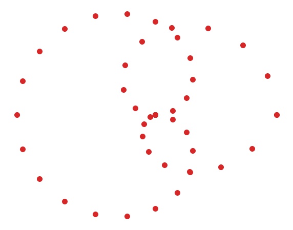
(a)

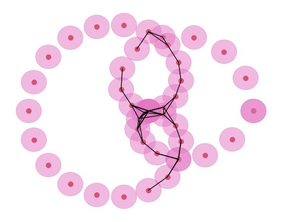
(b)

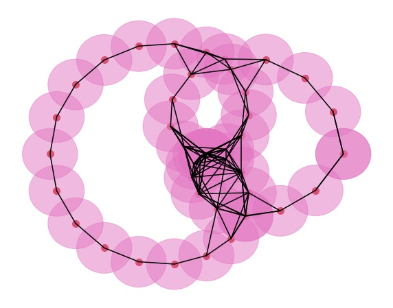
(c)

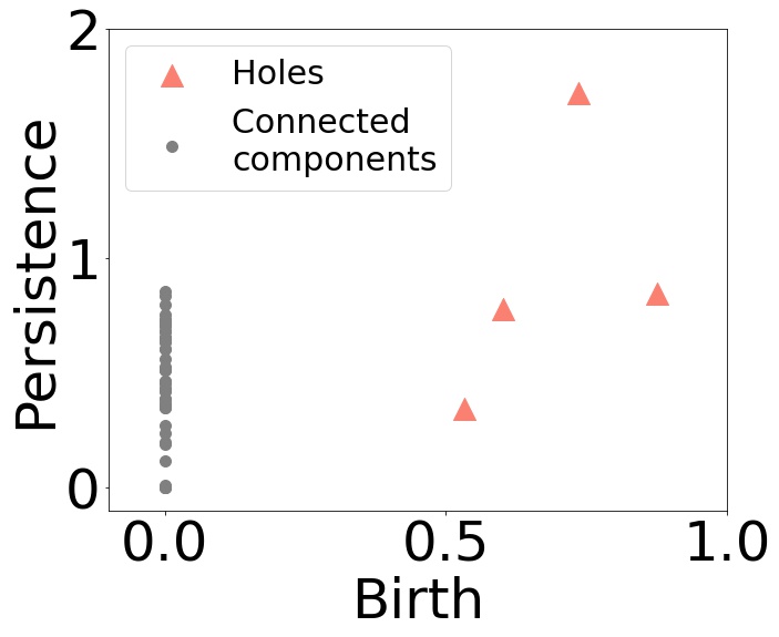
(d)

Figure 1: (a) A point cloud with 45 (red) points. (b) A Vietoris-Rips complex of the point cloud in (a) for radius $\zeta_{i}$. (c) Another Vietoris-Rips complex of the point cloud in (a), with radius $\zeta_{j}>\zeta_{i}$. (d) A tilted PD for connected components and holes associated with a sequence of Vietoris-Rips complexes.

Definition 1.

A $\psi$-dimensional collection of data $\{v_{0},\dots,v_{\tau}\}\subset\mathbb{R}^{\psi}\setminus\{0\}$ is said to be geometrically independent if for any set $t_{i}\in\mathbb{R}$ with $\sum_{i=0}^{\tau}t_{i}=0$, the equation $\sum_{i=0}^{\tau}t_{i}v_{i}=0$ implies that $t_{i}=0$ for all $i\in\{0,\dots,\tau\}.$

Definition 2.

A $\kappa-$simplex, is a collection of $\kappa+1$ geometrically independent elements with their convex hull

$$[v_{0},\dots,v_{\kappa}]=\Big{\{}\sum_{i=0}^{\kappa}\omega_{i}v_{i}:\sum_{i=0}^{\kappa}\omega_{i}=1\Big{\}}.$$

We say that the vertices $v_{0},\dots,v_{\tau}$ span the $\kappa-$dimensional simplex, $[v_{0},\dots,v_{\kappa}]$. The faces of a $\kappa-$simplex $[v_{0},\dots,v_{\kappa}]$, are the $(\kappa-1)-$simplices spanned by subsets of $\{v_{0},\dots,v_{\kappa}\}$.

Definition 3.

A simplicial complex $S_{c}$ is a collection of simplices satisfying two conditions: (i) if $\xi\in S_{c}$, then all faces of $\xi$ are also in $S_{c}$, and (ii) the intersection of two simplices in $S_{c}$ is either empty or contained in $S_{c}$.

Given a point cloud, $V$, our goal is to construct a sequence of simplicial complexes that reasonably approximates the underlying shape of the data. We accomplish this by using the Vietoris-Rips filtration.

Definition 4.

Let $V=\{v_{0},\ldots,v_{\tau}\}$ be a point cloud in $\mathbb{R}^{\psi}$ and $\zeta>0$. The Vietoris-Rips complex of $V$ is defined to be the simplicial complex $\mathcal{V}_{\zeta}(V)$ satisfying $[v_{i_{1}},\dots,v_{i_{l}}]\in\mathcal{V}_{\zeta}(V)$ if and only if $\operatorname{diam}(v_{i_{1}},\dots,v_{i_{l}})<\zeta$. Given a nondecreasing sequence $\{\zeta_{\tau}\}\in\mathbb{R}^{+}\cup\{0\}$ with $\zeta_{0}=0$, we denote its Vietoris-Rips filtration by $\{\mathcal{V}_{\zeta_{\tau}}(V)\}_{\tau\in\mathbb{N}}$.

A PD $\mathcal{D}$ is a multi–set of points in $\mathbb{W}\times\{0,1,\dots,\psi-1\}$, where

$$\mathbb{W}=\{d=(\beta,\delta-\beta)\in\mathbb{R}^{2}\mid\beta,\delta-\beta\geq 0\}.$$ (1)

For a fixed dimension $\kappa=0,\dots,\psi-1$, each element $(\beta,\delta-\beta)$ represents a homological feature of dimension $\kappa$ that appears at scale $\beta$ during a Vietoris-Rips filtration, and disappears at scale $\delta$. In other words, the homological feauture $(\beta,\delta-\beta)$ is a $\kappa-$dimensional hole that persists $\delta-\beta$. Features with $\kappa=0$ correspond to connected components, $\kappa=1$ to loops, and $\kappa=2$ to voids. An illustration of Vietoris-Rips filtration and an example of a PD is given in Figure 1.

2.1.2 Filtration from functions

For a real number $\epsilon$, the sublevel set $S_{\epsilon}$ of a function, $f:\mathbb{R}\rightarrow\mathbb{R}$, is defined as $S_{\epsilon}=f^{-1}((-\infty,\epsilon])$. A collection $\{S_{\epsilon}:\epsilon\in\mathbb{R}\}$ of sublevel sets of $f$ is called a sublevel set filtration of $f$. A sublevel set filtration tracks the evolution of connected components, that is of zero-dimensional homological features, as ${\epsilon}$ increases. As all of the sublevel sets $S_{\epsilon}$ are either empty or a union of intervals, we can extract information about the connectivity of the sets $S_{\epsilon}$, which in turn provides the number of connected components. We record the value of $\epsilon$ (local minimum of $f$) at which a given connected component is born, and the value of $\epsilon$ (local maximum of $f$) at which the connected component disappears by merging with a pre-existing connected component. According to the elder rule Edelsbrunner2010 , whenever two connected components merge, the one born later disappears while the one born earlier persists. Once $\epsilon$ takes the maximum value $\max f(t)$, all the sublevel sets merge into a single connected component.

For every connected component that arises in the filtration, we track the points $({\beta},{\delta})\in\mathbb{R}^{2}$, where $\beta$ is the value of $\epsilon$ at which the connected component is born and $\delta$ is the value of $\epsilon$ at which it disappears, and call the resulting collection a PD. Similarly to Section 2.1.1, one may apply the linear transformation $d=(\beta,\delta-\beta)$ and consider the associated wedge $\mathbb{W}$. An illustration of a sublevel set filtration of a function and of the tilted PD based on the filtration are shown in Figure 2.

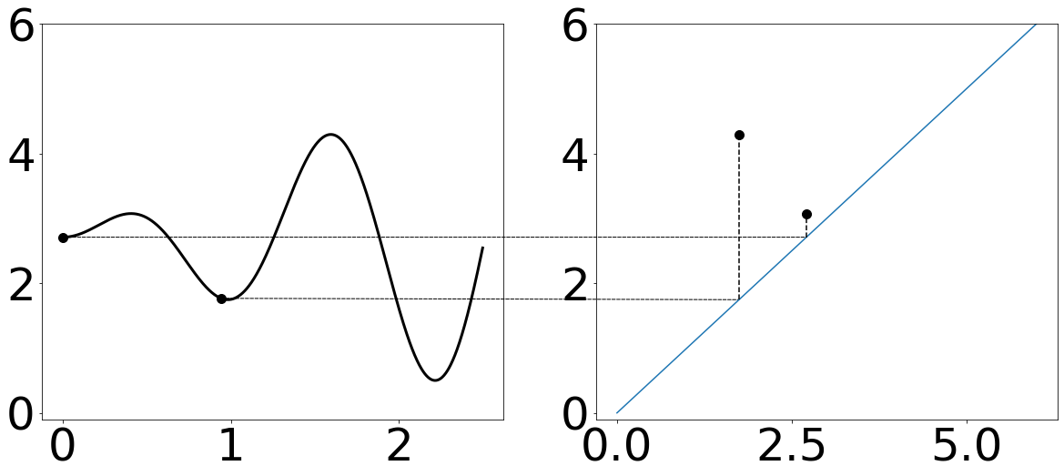
(a)

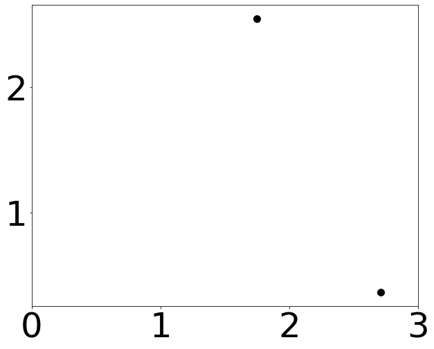
(b)

Figure 2: (a) A continuous function and the PD of its sublevel set filtration. (b) The tilted PD obtained from the sublevel set filtration.

2.2 PIPPs

Here, we present the components that we later employ in Section 3 to construct our RPDG framework. Section 2.2.1 states the definition of a pairwise interacting point process (PIPP), including the probability density function (pdf) of a set of points in the PIPP. Sections 2.2.2 and 2.2.3 provide a spatial pattern and a pairwise interaction function, respectively, that can be used to fully specify the pdf of a set of ponts in a PIPP. Our PIPP model for PDs (Section 3.1) and our RJ-MCMC algorithm that samples PDs using our model (Section 3.3) are built upon the PIPP density specified across Sections 2.2.1, 2.2.2 and 2.2.3. The PIPP pseudolikelihood of Section 2.2.4 is used for inferring the parameters of our PIPP model for PDs, as elaborated in Section 3.2.

2.2.1 PIPP density

One of our central motivations is to capture the local and global spatial features of the distribution of points in a PD. A PIPP is a Gibbs point process with density function determined by a first and second order potential function Baddeley2000 . In the context of a PD, the first order potential function captures the spatial density of points in the PD and the second order potential function determines interactions between all possible pairs of points.

Definition 5 (PIPP).

Let $(\mathbb{W},\mathcal{W},\lambda)$ be a measure space, where $\mathbb{W}$ is the set defined in Equation (1), and in addition, a bounded region of $\mathbb{R}^{2}$, $\mathcal{W}$ is the Borel $\sigma$-algebra on $\mathbb{W}$, and $\lambda$ is the Lebesgue measure. A pairwise interacting point process $X$ is a spatial point process on $(\mathbb{W},\mathcal{W},\lambda)$ with spatial pattern function $s:\mathbb{W}\rightarrow\mathbb{R}^{+}\cup\{0\}$ and interaction function $h_{\theta}:\mathbb{W}\times\mathbb{W}\rightarrow\mathbb{R}^{+}\cup\{0\}$. For a set of points $\mathbf{x}=\{x_{1},\dots,x_{n}\}\subseteq\mathbb{W}$ of $X$, the pdf $f(\mathbf{x}\mid\theta)$ of $\mathbf{x}$ has the form

$$f(\mathbf{x}\mid\theta) =\frac{1}{Z(\theta)}\prod_{i=1}^{n}s(x_{i})g(\mathbf{x}\mid\theta),$$ (2)

$$g(\mathbf{x}\mid\theta) =\prod_{i<j}h_{\theta}(x_{i},x_{j}),$$ (3)

where $\theta=(\theta_{1},\dots,\theta_{k})\in\mathbb{R}^{k}$ is a vector of parameters, and $Z(\theta)=\int_{\mathbb{W}}\prod_{i=1}^{n}s(x_{i})g(\mathbf{x}\mid\theta)\,d\lambda(\mathbf{x}),$ is the normalizing constant.

According to Definition 5, a PIPP is a spatial point process. Thus, the number of points of a PIPP in any region $R\subseteq\mathbb{W}$ follows a Poisson distribution with mean $\lambda(R)$. The normalizing constant $Z(\theta)$ is typically intractable, i.e. it is not available in closed form or it is computationally expensive. An example of interaction function $h_{\theta}$ of Equation (3) and the associated parameter vector $\theta$ are given in Section 2.2.3. More specifically, see Equation (5).

2.2.2 A spatial pattern function

One way of specifying the spatial pattern function $s$ in Equation (2) is based on the notion of Voronoi diagrams. Along these lines, we recall what is a Voronoi cell (Definition 6), which constitutes a building block for a Voronoi diagram (Definition 7). Subsequently, we state the spatial pattern induced by a Voronoi diagram (Definition 8).

Definition 6 (Voronoi cell).

Let $\{x_{1},\dots,x_{n}\}$ be a set of distinct points in a bounded region $\mathbb{W}$ of $\mathbb{R}^{2}$. The Voronoi cell $T_{i},\leavevmode\nobreak\ i=1,\ldots,n$, associated with $x_{i}$ is defined as

$$T_{i}=\{x\in\mathbb{W}:\|x-x_{i}\|\leq\|x-x_{j}\|\,\,\forall\,\,j\leavevmode\nobreak\ \mbox{with}\leavevmode\nobreak\ j\neq i\},$$

where $\|\cdot\|$ denotes the Euclidean norm.

Definition 7 (Voronoi diagram).

Let $\{x_{1},\dots,x_{n}\}$ be a set of distinct points in a bounded region $\mathbb{W}$ of $\mathbb{R}^{2}$. Moreover, let $T_{i},\leavevmode\nobreak\ i=1,\ldots,n$, be the Voronoi cell associated with $x_{i}$. The Voronoi diagram associated with $\{x_{1},\ldots,x_{n}\}$ is defined as the collection $\{T_{1},\ldots,T_{n}\}$ of Voronoi cells.

A Voronoi cell $T_{i}$ has the property that any point in the interior of $T_{i}$ is closer to point $x_{i}$ than to any other point $x_{j},\leavevmode\nobreak\ j\neq i$ Okabe2000 . RJ-MCMC for PDs, as discussed in Section 3.3, samples almost surely from the Voronoi cell interiors.

Definition 8 (Spatial pattern induced by a Voronoi diagram).

Let $\{T_{1},\ldots,T_{n}\}$ be the Voronoi diagram associated with a set of points $\{x_{1},\dots,x_{n}\}$ in a bounded region $\mathbb{W}$ of $\mathbb{R}^{2}$. Let $A_{i},\leavevmode\nobreak\ i=1,\ldots,n$, be the area of Voronoi cell $T_{i}$. The spatial pattern function $s:\mathbb{W}\rightarrow\mathbb{R}^{+}\cup\{0\}$ induced by $\{T_{1},\ldots,T_{n}\}$ is defined as

$$s(x)=\sum_{l=1}^{n}A_{l}\mathbbm{1}_{\{x\in T_{l}\}},$$ (4)

where $x\in\mathbb{W}$, and $\mathbbm{1}_{\{\cdot\}}$ denotes the indicator function.

Consider a PIPP with points $\{x_{1},\dots,x_{n}\}$. The PIPP pattern function $s$ in Equation (2) can be set via the Voronoi diagram associated with points $\{x_{1},\dots,x_{n}\}$. For a PIPP point $x_{i}\in T_{i},\leavevmode\nobreak\ i=1,\ldots,n$, it follows from Equation (4) that $s(x_{i})=A_{i}$, where $A_{i}$ is the area of cell $T_{i}$.

2.2.3 A pairwise interaction function

The interaction term $h_{\theta}(x_{i},x_{j})$ in Equation (3) is chosen typically so that it depends on the Euclidean distance $\|x_{i}-x_{j}\|$ and on parameter $\theta$. The piece-wise constant pairwise interaction function (Definition 9) can be used in Equation (3) as the interaction function $h_{\theta}$ for pairs of points in a PIPP. This is also known as the multi-scale generalization of the Strauss interaction strauss1975 .

Definition 9 (Piece-wise constant pairwise interaction function).

Let $\mathbb{W}$ be a bounded region in $\mathbb{R}^{2}$. The piece-wise constant pairwise interaction function $h_{\theta}:\mathbb{W}\times\mathbb{W}\rightarrow\mathbb{R}^{+}\cup\{0\}$ is defined as

$$h_{\theta}(x,z)=\exp\left(\sum_{l=1}^{k}\theta_{l}{\mathbbm{1}_{\{r_{l-1}<\|x-z\|\leq r_{l}\}}}\right),$$ (5)

where $(x,z)\in\mathbb{W}\times\mathbb{W}$, $r_{l}\in\mathbb{R}$ for $l=0,1,\ldots,k$, satisfying $0=r_{0}<r_{1}<\ldots<r_{k}$, and $\mathbbm{1}_{\{\cdot\}}$ denotes the indicator function. The vector $\mathbf{r}=(r_{1},\dots,r_{k})$ is called the vector of jump points.

The interaction function of Equation (5) is a piece-wise constant function, whose value $h_{\theta}(x,z)$ depends only on the distance between $x$ and $z$; if $r_{l-1}<\|x-z\|\leq r_{l}$, then $h(x,z)=\exp(\theta_{l})$. We thus interpret the jump points $r$ as points of discontinuity of $h_{\theta}$, and the parameter vector $\theta$ as a set of weights that determines how important is the interaction among PD points.

2.2.4 PIPP log-pseudolikelihood

The density $f(\mathbf{x}\mid\theta)$ given by Equation (2) can be employed as a likelihood function. A PIPP likelihood function $f(\mathbf{x}\mid\theta)$, as specified by Equation (2), is computationally expensive, since the normalizing constant $Z(\theta)$ is intractable. A pseudolikelihood can be used as a computationally feasible approximation of $f(\mathbf{x}\mid\theta)$. According to Baddeley2000 , we state the pseudolikelihood of a PIPP (Definition 11) based on the conditional intensity of the PIPP (Definition 10).

Definition 10 (PIPP conditional intensity).

Let $\mathbf{x}=\{x_{1},\ldots,x_{n}\}$ be a set of points of a PIPP $X$ with density $f(\mathbf{x}\mid\theta)$, where $\theta=(\theta_{1},\dots,\theta_{k})\in\mathbb{R}^{k}$. The conditional intensity of $X$ is defined as

$$\mathcal{I}(u,\mathbf{x})=\left\{\begin{array}[]{ll}\frac{f(\mathbf{x}\cup{u}\mid\theta)}{f(\mathbf{x}\mid\theta)}&u\notin\mathbf{x}\\ \frac{f(\mathbf{x}\mid\theta)}{f(\mathbf{x}\setminus{u}\mid\theta)}&u\in\mathbf{x}.\end{array}\right.$$ (6)

For a PIPP $X$ on $(\mathbb{W},\mathcal{W},\lambda)$, the conditional intensity $\mathcal{I}(u,\mathbf{x})$ is the conditional probability that $X$ has a point $u$ in $\mathbb{W}$ given that $X$ consists of $\mathbf{x}$. For the PIPP density of Equation (2), the conditional intensity takes the form

$$\mathcal{I}(u,\mathbf{x}\mid\theta)=s(u)\prod_{\mathclap{\begin{subarray}{c}i=1\\ x_{i}\neq u\end{subarray}}}^{n}h_{\theta}(u,x_{i}),$$ (7)

Definition 11 (PIPP log-pseudolikelihood).

The log-pseudolikelihood of a PIPP $X$ with conditional intensity $\mathcal{I}(u,\mathbf{x}\mid\theta)$ is defined as

$$\log\tilde{L}(\theta\mid\mathbf{x})=$$

$$\sum_{i=1}^{n}\log\mathcal{I}(x_{i},\mathbf{x}\mid\theta)-\int_{\mathbb{W}}\mathcal{I}(u,\mathbf{x}\mid\theta)du.$$ (8)

If the conditional intensity $\mathcal{I}$ in Equation (8) employs the piece-wise constant pairwise interaction function, then the PIPP log-pseudolikelihood can be approximated by the Berman-Turner device Berman1992 ; Baddeley2000 . The PIPP log-pseudolikelihood approximation based on the Berman-Turner device is given by

$$\log\tilde{L}(\theta\mid\mathbf{x})\approx$$

$$\sum_{j=1}^{m}\mathbbm{1}_{\{u_{j}\in\mathbf{x}\}}\log\mathcal{I}(u_{j},\mathbf{x}\mid\theta)-w_{j}\mathcal{I}(u_{j},\mathbf{x}\mid\theta),$$ (9)

where $\{u_{1},\ldots,u_{m}\}$ are points in $\mathbb{W}$ such that $\{x_{1},\ldots,x_{n}\}\subseteq\{u_{1},\ldots,u_{m}\}$, and $\{w_{1},\ldots,w_{m}\}$ are positive weights summing to the area of $\mathbb{W}$.

2.3 Motivation for RJ-MCMC

The idea of sampling PDs to perform statistical inference was introduced by Adler2017 and was improved in Adler2019 . In Adler2017 ; Adler2019 , a Metropolis-within-Gibbs (MWG) algorithm was constructed to sample PDs by randomly relocating PD points. However, relocating points of a PD is not the only move one may consider. For example, one may observe more or fewer number of points in a PD depending on the noise level in the data.

In this paper, we construct an RJ-MCMC algorithm to sample PDs. RJ-MCMC is an MCMC algorithm developed by Green1995 to enable simulation from a distribution on spaces of varying dimensions. In the context of PDs, RJ-MCMC enables additional types of stochastic moves in comparison to the MWG approach of Adler2017 ; Adler2019 . More specifically, we develop an RJ-MCMC algorithm which generates new PDs not only by relocating points, but also by adding or removing points. The addition or removal of points generates PDs with different number of points. Our RJ-MCMC scheme solves the problem of sampling from a distribution of PDs with varying number of points, in contrast to the MWG scheme of Adler2017 ; Adler2019 , which solves the problem of sampling from a distribution of PDs with a given fixed number of points.

Our RJ-MCMC approach provides two benefits. Firstly, the larger space of PDs associated with RJ-MCMC yields samples of PDs that adhere more closely to topological features present in a given dataset; for a more concrete quantification of this argument, see Section 4.2. Secondly, the number of points in a PD is an unknown hyperparameter in the presence of noisy data. RJ-MCMC samples PDs without conditioning on a specific value of this hyperparameter. Hence, uncertainty associated with the number of PD points is automatically accounted for by RJ-MCMC.

3 Methodology

In this section, we present our proposed methodology. More specifically, we introduce a PIPP model for PDs based on pairwise interactions of PD points (Section 3.1), a method for inferring the parameters of the model (Section 3.2), and a RJ-MCMC algorithm to sample PDs represented by the model (Section 3.3).

3.1 Modeling PDs as PIPPs

In Definition 12, we introduce the PIPP representation of a PD. Subsequently, we specify the spatial density of PD points and the interaction function between pairs of PD points in this PIPP representation of a PD.

Definition 12 (PIPP representation of a PD).

Let $D=(d_{1},\dots,d_{n})$ be a PD in the wedge $\mathbb{W}$ as defined in Equation (1). We assume that the points $(d_{1},\dots,d_{n})$ of $D$ admit a PIPP on $(\mathbb{W},\mathcal{W},\lambda)$ with pdf $f(D\mid\theta)$. According to Equations (2) and  (3), the PIPP density of $D$ is given as follows

$$f(D\mid\theta)=\frac{1}{Z(\theta)}\prod_{i=1}^{n}s(d_{i})\prod_{i<j}h_{\theta}(d_{i},d_{j}).$$ (10)

where $\theta\in\mathbb{R}^{k}$ is a parameter vector. $Z(\theta)$ is the normalizing constant of $f(D\mid\theta)$.

In Equation (10), the points $(d_{1},\dots,d_{n})$ in $D$ admit a spatial pattern function $s$ induced by the Voronoi diagram $\{T_{1},\ldots,T_{n}\}$, where $T_{i},\leavevmode\nobreak\ i=1,\ldots,n$, is the Voronoi cell associated with point $d_{i}$. The interaction $h_{\theta}(d_{i},d_{j})$ between two points $d_{i}$ and $d_{j}$ of $D$ appears in Equation (10). We hereafter set $h_{\theta}(d_{i},d_{j})$ to be the piece-wise constant pairwise interaction given by Equation (5).

3.2 Parameter estimation

The PIPP density value $f(D\mid\theta)$ of a PD $D$ is given by Equation (10). Our goal is to sample PDs from the PIPP density $f(\cdot\mid\theta)$. In other words, we aim at sampling PDs that share the same distribution of points with $D$. We do not have knowledge of parameter $\theta$, so in this section we provide a way of obtaining an estimator $\hat{\theta}$ of $\theta$. Given $\hat{\theta}$, we construct an RJ-MCMC sampler that generates PDs from the target PIPP density $f(\cdot\mid\hat{\theta})$ in Section 3.3.

To estimate $\theta$, all the available information is encoded in the PD, $D,$ generated from a given dataset. Recalling that the points of $D$ admit a PIPP representation, an approximate estimator $\hat{\theta}$ of $\theta$ can be acquired based on the Berman-Turner approach according to Equation (9). More specifically, $\hat{\theta}=\operatorname*{argmax}_{\theta}\log\tilde{L}(\theta\mid D)$ is computed by maximizing the approximate log-pseudolikelihood

$$\log\tilde{L}(\theta\mid D)\approx$$

$$\sum_{j=1}^{m}\mathbbm{1}_{\{u_{j}\in D\}}\log\mathcal{I}(u_{j},D\mid\theta)-A_{j}\mathcal{I}(u_{j},D\mid\theta),$$

where $\{u_{1},\ldots,u_{m}\}$ are points in the wedge $\mathbb{W}$ in which $D$ lives, satisfying $D\subseteq\{u_{1},\ldots,u_{m}\}$. A Voronoi cell $T_{j},\leavevmode\nobreak\ j=1\ldots,m$, of area $A_{j}$ is associated with point $u_{j}$, making up a Voronoi diagram $\{T_{1},\ldots,T_{m}\}$. The area $\sum_{j=1}^{m}A_{j}$ is equal to the area of $\mathbb{W}$. The conditional intensities $\mathcal{I}(u_{j},D\mid\theta)$ are given by Equation (7), where $s$ is the spatial pattern function induced by $\{T_{1},\ldots,T_{m}\}$.

The points $\{u_{1},\ldots,u_{m}\}\setminus D$, which are additional points not in $D$, constitute a hyperparameter. If $D$ is a dense PD, then a practical choice is to set $\{u_{1},\ldots,u_{m}\}\setminus D=\varnothing$ and therefore $\{u_{1},\ldots,u_{m}\}=D$. If $D$ is a sparse PD with a relatively small number of points, it is possible to augment it with synthetic points, in which case $\{u_{1},\ldots,u_{m}\}$ is a strict superset of $D$ containing the original points in $D$ and the synthetic points $\{u_{1},\ldots,u_{m}\}\setminus D$. Irrespective of how the hyperparameter $\{u_{1},\ldots,u_{m}\}\setminus D$ is tuned, it is used only to compute $\hat{\theta}$.

Subsequently, samples are drawn from the target density $f(\cdot\mid\hat{\theta})$, as explained in Section 3.3 by using the estimated value $\hat{\theta}$. In other words, the PIPP log-pseudolikelihood of Definition 11 is used for acquiring the estimate $\hat{\theta}$ only, and it is not used in the sampling process. Having obtained $\hat{\theta}$, the PIPP density $f(\cdot\mid\hat{\theta})$ of Definition 12 becomes the target density from which PD samples are drawn via RJ-MCMC.

3.3 Sampling PDs

The key contribution of this work is an RJ-MCMC algorithm for generating random samples of PDs modeled as pairwise interaction point processes. Notably, our RJ-MCMC algorithm can be utilized to perform inference based on topological features elicited via PD augmentation, especially when the sample size of a given dataset is relatively small. This section starts by outlining the three types of moves allowed by RJ-MCMC in the space of PDs and by providing an informal description of the RJ-MCMC acceptance probabilities for these moves. Subsequently, it states formally the RJ-MCMC sampling scheme.

3.3.1 RJ-MCMC for PDs: outline

Our RJ-MCMC sampler explores the PD space via three moves; (i) a point in a PD can be moved from one location to another without changing the total number of points, (ii) a point can be added to a PD, and (iii) a point can be removed from a PD. In particular, the sampling process consists of two types of MCMC updates. A MWG update relocates points in a PD via random-walk Metropolis steps, similar to Adler2017 . Furthermore, an RJ-MCMC update adds a point to the PD or removes a point from it, thus yielding a novel PD sampler.

The probabilities of changing the location of a selected point, of adding a new point, and of removing a selected point are denoted by $p_{m}$, $p_{a}$, and $p_{r}$, respectively. At each RJ-MCMC iteration, a type of move is chosen randomly according to a categorical distribution $\text{Categorical}(p_{m},p_{a},p_{r})$ with event probabilities $p_{m}$, $p_{a}$, and $p_{r}$.

Let $D^{(l)}=(d_{1}^{(l)},\dots,d_{\lvert D^{(l)}\rvert}^{(l)})$ be the current PD with $\lvert D^{(l)}\rvert$ points at the $l$-th RJ-MCMC iteration. A type of move is chosen according to $\text{Categorical}(p_{m},p_{a},p_{r})$. Subsequently, a candidate PD $D^{*}$ is proposed subject to the type of chosen move. If it is chosen to relocate the points of $D^{(l)}$, then a new location $d_{i}^{*}$ is sampled from a proposal density $q$ and the candidate PD is set to $D^{*}=(d_{1}^{(l)},\dots,d_{i-1}^{(l)},{d_{i}}^{*},d_{i+1}^{(l)},\dots,d_{\lvert D^{(l)}\rvert}^{(l)})$ for each $i=1,\ldots,\lvert D^{(l)}\rvert$. If it is chosen to add a new point $d^{*}$ to $D^{(l)}$, then $d^{*}$ is sampled uniformly in the support of the underlying point process representing $D^{(l)}$ and the candidate PD is set to $D^{*}=(D^{(l)},d^{*})$. If it is chosen to remove a point $d^{*}$ from $D^{(l)}$, then a point $d^{*}=d^{(l)}_{i}\in D^{(l)}$ is chosen randomly and the candidate PD is set to $D^{*}=D^{(l)}\setminus d^{*}$.

Once a candidate PD $D^{*}$ has been proposed, it is accepted with probability $a(D^{(l)},D^{*})$. If $D^{*}$ is accepted, then the PD at iteration $l+1$ is set to $D^{(l+1)}=D^{*}$, otherwise $D^{(l+1)}=D^{(l)}$. In the case of point relocation, $a(D^{(l)},D^{*})$ is a typical Metropolis-Hastings acceptance probability. In the case of point addition or removal, $a(D^{(l)},D^{*})$ is a reversible jump acceptance probability (see Proposition 1). An RJ-MCMC algorithm for sampling pairwise interacting point processes is introduced by Geyer1994 and is adapted in the present paper to sample PDs. As part of this adaptation, Lemma 1 is stated by modifying a corresponding lemma for point processes in Geyer1994 to fit the context of sampling PDs, which are represented by PIPP densities (see Definition 5).

Lemma 1.

Let $D$ be a PD with $\lvert D\rvert$ points, which admit a PIPP density $f(\cdot\mid\theta)$ given by Equation (10). Moreover, it is assumed that the number of points of $D$ in a region $R$ has a Poisson distribution with mean $\lambda(R)$.

Let $d^{*}$ be a point candidate for addition to $D$. Assume that $d^{*}$ has distribution $\frac{\lambda(\cdot)}{\lambda(R)}$. The acceptance probability for the candidate PD $D^{*}=(D,d^{*})$ is

$$a(D,D^{*})=\frac{f(D^{*}\mid\theta)\lambda(R)}{f(D\mid\theta)(\lvert D\rvert+1)}.$$ (11)

If $D=\varnothing$ then the PD chain stays at $D$. Otherwise, let $d^{*}\in D$ be a point candidate for removal from $D$. The acceptance probability for the candidate PD $D^{*}=D\setminus d^{*}$ is

$$a(D,D^{*})=\frac{f(D^{*}\mid\theta)(\lvert D\rvert-1)}{f(D\mid\theta)\lambda(R)}.$$ (12)

3.3.2 RJ-MCMC for PDs: construction

Proposition 1 states the acceptance probabilities for the three types of moves in the proposed RJ-MCMC scheme. The proof of Proposition 1 follows from Lemma 1 and is available in Appendix A. As a brief and informal outline of the proof, the acceptance probability (13) follows from a Metropolis-Hastings step for point relocation, while the acceptance probabilities (14) and (15) for point addition and point removal follow from the reversible jump acceptance probabilities (11) and (12) of Lemma 1, respectively.

Proposition 1.

Consider a random PD on the wedge $\mathbb{W}$ modeled by a PIPP density $f(\cdot\mid\widehat{\theta})$ given by Equation (10). The number of points of a PD in a region $\mathbb{W}$ has a Poisson distribution with mean $\lambda(\mathbb{W})$. Let $D^{(l)}=(d_{1}^{(l)},\dots,d_{\lvert D^{(l)}\rvert}^{(l)})$ be the PD at the $l$-th MCMC iteration. The acceptance probabilities for generating random PDs from $f(\cdot\mid\widehat{\theta})$ by relocating, adding or removing points follow.

Let $D^{*}=(d_{1}^{(l)},\dots,d_{i-1}^{(l)},{d_{i}}^{*},d_{i+1}^{(l)},\dots,d_{\lvert D^{(l)}\rvert})$ be the candidate PD for the relocation move, where $d_{i}^{*}$ is chosen according to a proposal density $q$. The acceptance probability for $D^{*}$ is

$$a(D^{(l)},D^{*})=$$

$$\min\left\{1,\frac{s({d_{i}}^{*})g({D^{*}\mid\widehat{\theta}})q({d_{i}}^{(l)})}{s({d_{i}}^{(l)})g({D^{(l)}\mid\widehat{\theta}})q({d_{i}}^{*})}\right\},$$ (13)

For the addition of a point $d^{*}$ to $D^{(l)}$, we choose $d^{*}$ uniformly at random in $\mathbb{W}$ and obtain the candidate PD $D^{*}=(D^{(l)},d^{*})$. The acceptance probability for $D^{*}$ is

$$a(D^{(l)},D^{*})=$$

$$\min\left\{1,\frac{\left[\prod_{i=1}^{|D^{(l)}|}h_{\widehat{\theta}}(d^{(l)}_{i},d^{*})\right]s(d_{i}^{*})\lambda{(\mathbb{W})}}{|D^{(l)}|+1}\right\}.$$ (14)

For the removal of a point $d_{i}^{(l)}$ from $D^{(l)}$, we choose uniformly at random $d_{i}^{(l)}$ and obtain the candidate PD $D^{*}=D^{(l)}\setminus d^{(l)}_{i}$. The acceptance probability for $D^{*}$ is

$$a(D^{(l)},D^{*})=$$

$$\min\left\{1,\frac{|D^{(l)}|-1}{\left[\prod_{j\neq i}h_{\widehat{\theta}}(d^{(l)}_{j},d_{i}^{(l)})\right]s(d_{i}^{(l)})\lambda{(\mathbb{W})}}\right\}.$$ (15)

The pseudocode of the RJ-MCMC sampler for generating PDs is summarized by Algorithm 1. Section 4.2 provides an experimental validation of the relative advantages of Algorithm 1 in comparison to a MWG sampler of PDs with fixed number of points Adler2019 .

Algorithm 1 RJ-MCMC sampling of PDs

1:Input: initial PD $D^{(0)}=(d_{1}^{(0)},\dots,d_{|D^{0}|}^{(0)})$

2:Input: probabilities $(p_{m},p_{a},p_{r})$

3:

4:for $l\in\{1,...,N\}$ do

5:     Sample $\gamma$ from $\mbox{Categorical}(p_{m},p_{a},p_{r})$

6:     

7:     if $\gamma=1$ then

8:         Choose $i$ randomly from 1 to $|D^{(l)}|$

9:         Sample $d_{i}^{*}$ from proposal density $q$

10:         $D^{*}=(d_{1}^{(l)},\dots,d_{i}^{*},\ldots,d_{|D^{(l)}|}^{(l)})$

11:         Compute $a(D^{(l)},D^{*})$ from Eq (13)

12:         Sample $u$ from uniform $\mathcal{U}(0,1)$

13:         if $u<a(D^{(l)},D^{*})$ then

14:              $D^{(l+1)}=D^{*}$

15:         else

16:              $D^{(l+1)}=D^{(l)}$

17:         end if

18:     else if $\gamma=2$ then

19:         Sample $d^{*}$ uniformly at random in $\mathbb{W}$

20:         $D^{*}=(D^{(l)},d^{*})$

21:         Compute $a(D^{(l)},D^{*})$ from Eq (14)

22:         Sample $u$ from uniform $\mathcal{U}(0,1)$

23:         if $u<a(D^{(l)},D^{*})$ then

24:              $D^{(l+1)}=D^{*}$

25:         else

26:              $D^{(l+1)}=D^{(l)}$

27:         end if

28:     else

29:         Sample a point $d^{*}_{i}$ from $D^{(l)}$

30:         $D^{*}=D^{(l)}\setminus d^{(l)}_{i}$

31:         Compute $a(D^{(l)},D^{*})$ from Eq (15)

32:         Sample $u$ from uniform $\mathcal{U}(0,1)$

33:         if $u<a(D^{(l)},D^{*})$ then

34:              $D^{(l+1)}=D^{*}$

35:         else

36:              $D^{(l+1)}=D^{(l)}$

37:         end if

38:     end if

39:end for

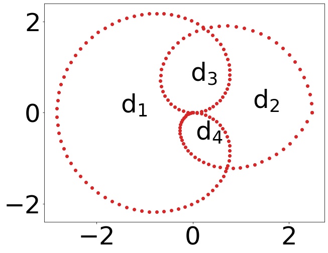
(a)

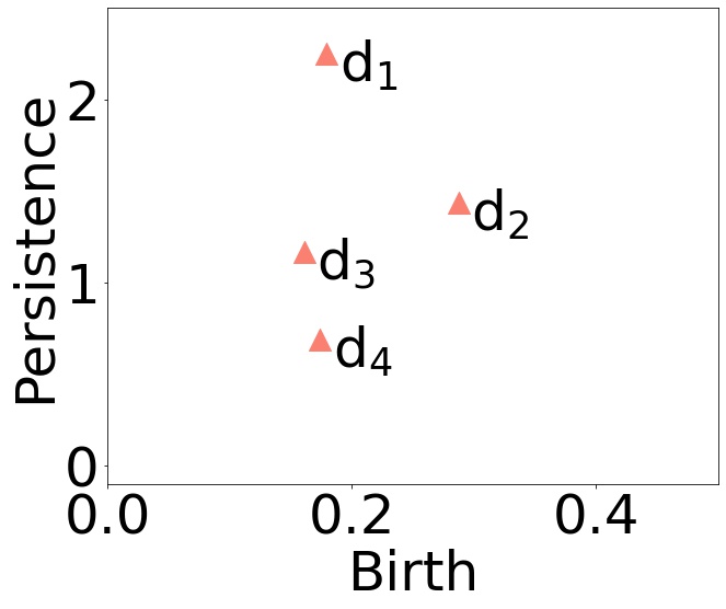
(b)

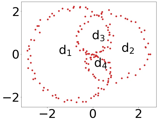
(c)

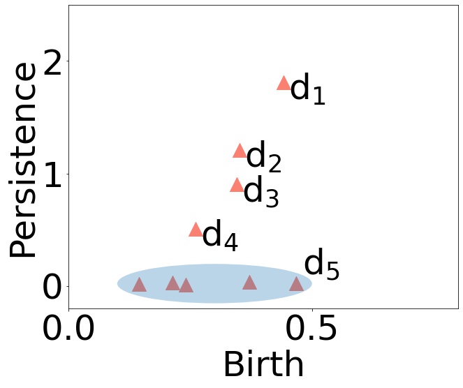
(d)

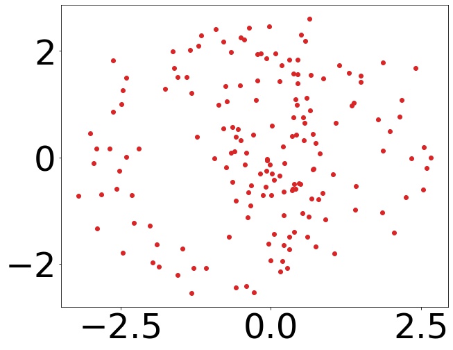
(e)

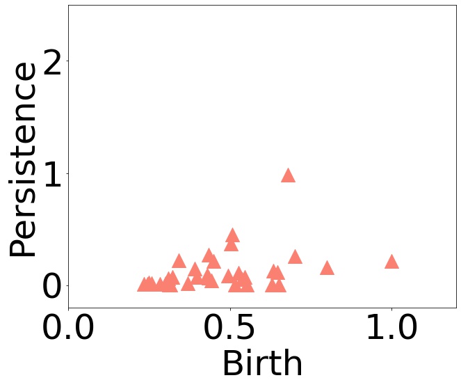
(f)

Figure 3: (a): a random sample of $170$ points from the asymmetric knot defined by Equation (16). (c) and (e): noisy versions of the random sample in (a), after adding noise to each point in (a), with noise having been drawn from a normal distribution centered at the point with variance $\sigma^{2}=0.005$ and $\sigma^{2}=0.1$, respectively. (a), (c) and (e) are displayed in Cartesian coordinates. (b), (d) and (f) are the PDs of one-dimensional features extracted from the simulated datasets in (a), (c) and (e), respectively. The PDs have been generated using Vietoris-Rips filtration, as discussed in Section 2.1.1.

4 Asymmetric knot example

In this section, we consider two noisy point cloud datasets shown in Figures 3c and 3e, which have been generated by adding normally distributed noise with respective variance $\sigma^{2}=0.005$ and $\sigma^{2}=0.1$, to the point cloud data of Figure 3a. The data of Figure 3a have been generated from the asymmetric knot

$$\text{knot}(\phi)=\begin{cases}\frac{7\sqrt{2}}{4}\cos\left(\frac{\phi}{2}\right),&0\leq\phi<\pi,\\ 2\sqrt{2}\cos\left(\frac{\phi}{2}\right),&\pi\leq\phi<3\pi,\\ \frac{7\sqrt{2}}{4}\left(\frac{\phi-3\pi}{\pi}\right)^{7/5},&3\pi\leq\phi<4\pi.\end{cases}$$ (16)

Figures 3b, 3d and 3f show the respective PDs of the noiseless point cloud (Figure 3a), of the point cloud with low level of noise ($\sigma^{2}=0.005$, Figure 3c) and of the point cloud with high level of noise ($\sigma^{2}=0.1$, Figure 3e). These PDs have been generated using Vietoris-Rips filtration (see Section 2.1.1). We focus on $1$-dimensional holes in the PDs shown in Figures 3b, 3d and 3f, as such holes characterize the prominent shape features of the asymmetric knot.

Section 4.1 deploys our RPDG algorithm to sample PDs from the PIPP density of the PD of Figure 3d. Section 4.2 compares RPDG with an existing PD sampling method Adler2019 ; for this comparison, we consider the point cloud data of Figure 3c and the corresponding PD of Figure 3d.

4.1 RPDG illustration

We illustrate how RPDG can be used to sample PDs from the target PIPP density of the PD of Figure 3d. In particular, Section 4.1.1 provides an example of how to setup RJ-MCMC sampling of PDs from the target PIPP density, while Section 4.1.2 introduces a notion of running average distance in the space of PDs to assess quality of PD sampling from a topological point of view. Section 4.1.3 presents some sensitivity analysis for the employed RJ-MCMC sampling scheme under different levels of noise in the original point cloud data from which the PD of Figure 3d has been generated.

4.1.1 RJ-MCMC sampling

The point cloud data in Figure 3c consist of four loops, each of different size. The corresponding PD in Figure 3d has four points $d_{i},\leavevmode\nobreak\ i=1,2,3,4$, associated with the loops of Figure 3c. Due to noise in the data of Figure 3c, several other PD points with lower persistence values are spawn, visualized inside the blue oval of Figure 3d. These PD points inside the blue oval do not correspond to any of the four topological features (loops), they are considered to be noise, and they are thus clustered together.

To sample PDs via RJ-MCMC as outlined by Algorithm 1, it is required to setup four components. More specifically, we specify a proposal density $q$ for sampling PD points, the target PIPP density $f(\cdot\mid\hat{\theta})$, the initial PD $D^{(0)}$ and probabilities $(p_{m},p_{a},p_{r})$.

We set the pertinent mixture $q(\cdot)=\sum_{i=1}^{5}w_{i}\mathcal{N}^{*}(\cdot\mid\mu_{i},\sigma_{i}^{2}\,I)$ as proposal density to sample a candidate PD point from the wedge $\mathbb{W}$ over which the PD of Figure 3d is defined. $\mathcal{N}^{*}$ is a bivariate truncated normal density supported on $\mathbb{W}$, $I$ is the identity matrix, $(\mu_{1},\mu_{2},\mu_{3},\mu_{4},\mu_{5})$ are the mixture component means, $(\sigma_{1}^{2},\sigma_{2}^{2},\sigma_{3}^{2},\sigma_{4}^{2},\sigma_{5}^{2})$ are the mixture component variances, and $(w_{1},w_{2},w_{3},w_{4},w_{5})$ are the mixture component weights. Table 3 in Appendix B shows the values of $\mu_{i},\sigma_{i}^{2}$ and $w_{i}$. This proposal mixture has been chosen empirically to capture the shape behavior of Figure 3d, as topologically expressed in the associated PD (Figure 3d); notice that the mixture component means $\mu_{i},\leavevmode\nobreak\ i=1,2,3,4$, of Table 3 are placed on the PD points $d_{i}$ of Figure 3d, while the fifth mean $\mu_{5}$ is placed on the blue oval of Figure 3d.

Appendix B provides the hyperparameters, whose values have been empirically set, for the target PIPP density $f(\cdot\mid\hat{\theta})$ of this section. We initialize Algorithm 1 by setting the PD of Figure 3d as the initial PD $D^{(0)}$ and by setting $p_{a}=p_{r}=p_{m}=1/3$. We then generate $N=100,000$ samples of PDs via Algorithm 1.

4.1.2 Running average distance

We introduce an empirical metric to assess the capacity of RPDG to sample PDs that preserve topological structure. To this end, we propose the running average distance between the persistence order statistics of the noiseless PD and the persistence order statistics of PDs generated via RPDG. Typically, the noiseless PD is not known given a dataset. However, in the controlled experimental setup of this RPDG illustration, we know the ground truth of noiseless PD (see Figure 3b).

Let $d^{\text{true},{(i)}}$ be the $i$-th largest persistence value of the points in the noiseless PD of Figure 3b. Moreover, let $d^{\text{sim},(i)}_{k}$ be the $i$-th largest persistence value of the points in the $k$-th PD sample of a realized chain of PDs, where $k=1,\ldots N$. We define the running average distance for the $i$-th largest persistence value up to the $n$-th PD sample to be

$$\mbox{dist}_{n}(i)=\frac{1}{n}\sum_{k=1}^{n}|d^{\text{sim},(i)}_{k}-d^{\text{true},{(i)}}|,$$ (17)

where $n=1,\ldots,N$. This distance has been chosen to examine the closeness of topologically prominent points in the simulated PDs to the four prominent points in the original PD. In Sections 4.1.3 and 4.2, we generate a trace plot of running average distance $\mbox{dist}_{n}(i)$ against RPDG (or MWG) iteration $n$ for each $i\in\{1,2,3,4\}$, since the noiseless PD of Figure 3b has four topologically prominent persistence values $d_{i},\leavevmode\nobreak\ i=1,2,3,4$.

The notion of running average distance can be applied to a real dataset by replacing the noiseless PD with the PD generated from a dataset. In such a case, the running average distance would quantify the distance of RPDG samples from the PD of the dataset.

4.1.3 Sensitivity analysis

Recall the two scenarios of point clouds with low and high noise given in Figures 3c and 3e, respectively, as well as their corresponding persistent diagrams in Figures 3d and 3f. For each noise level, we sample $100,000$ PDs via RPDG. Subsequently, we compute the running average distance given by Equation (17) for each of the four largest persistence values, as explained in Section 4.1.2, and display these distances in Figure 4.

In each of the four plots, RPDG converges in the sense that the distance of Equation (17) converges. As one may expect, the high noise example of Figure 3f produces the largest distance in the first and second largest persistence value in comparison to the low noise example of Figure 3d. In contrast, for the case of the third and fourth largest persistence value, the running average distance of the low noise case is larger than the one of the high noise case. This is not unexpected since the associated PD, depicted in Figure 3f, contains the majority of its points in the region of the underlying true PD points $d_{3}$ and $d_{4}$ (small loops); see Figure 3b. Thus, a large number of samples are drawn from that area, which in turn leads to a small deviation from the underlying ground truth.

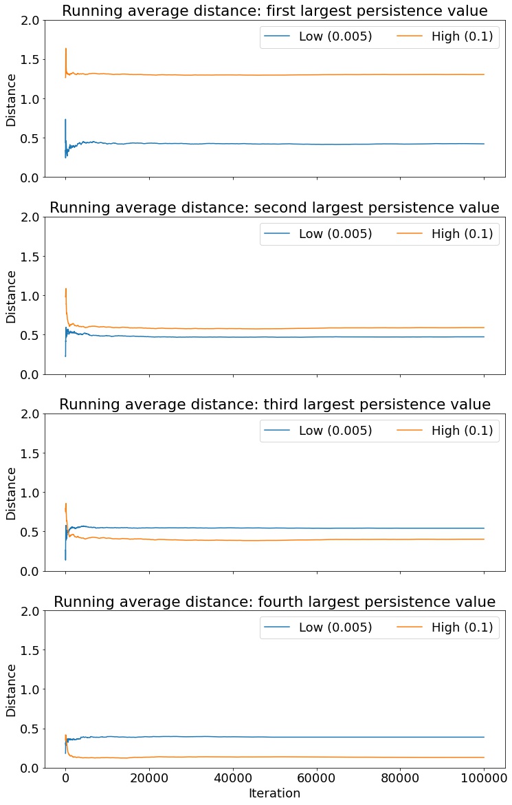
Figure 4: Sensitivity analysis for RPDG. Each plot displays three lines: a blue and orange line representing the running average distance for a persistence value using RPDG chains initialized at PDs associated with low ($\sigma^{2}=0.005$) and high ($\sigma^{2}=0.1$) levels of noise, respectively.

4.2 Comparison with MWG

In this section, we compare RPDG with the MWG sampling scheme proposed in Adler2019 . MWG has a set of hyperparameters, which have been empirically tuned. Subsequently, the parameters involved in MWG sampling are estimated in accordance with Adler2019 .

We sample $100,000$ PDs using MWG under the low level noise scenario, as the intention is to compare the ‘topological fidelities’ of RPDG and MWG for high quality data, that is for data relatively clean from noise admitting an underlying topological structure. We then compute the running average distance for each of the four largest persistence values based on MWG PD samples and on the noiseless PD of Figure 3b, as described in Section 4.1.2.

Figure 5 overlays the running average distance associated with RPDG and with MWG for each persistence value. The displayed running average distances are computed from one RPDG and one MWG chain realization, with both chains having the PD of Figure 3d as their initial state. While both sampling methods converge, RDPG enjoys lower distance from the ground truth in comparison to MWG.

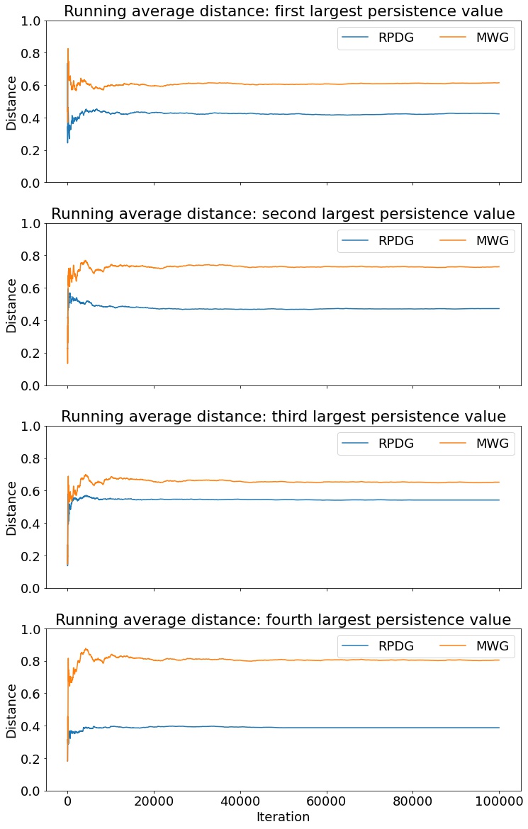
Figure 5: A comparison between RPDG and MWG. Each plot displays two lines: a blue line representing the running average distance for a persistence value based on RPDG samples and the noiseless PD of Figure 3b, and an orange line representing the running average distance for the same persistence value based on MWG samples and the noiseless PD of Figure 3b.

5 Materials science example

In this section, we consider a real materials science dataset collected in an experimental facility. Section 5.1 sets the stage by introducing the underlying materials science problem, while Section 5.2 describes the experimental data under consideration herein. Next a classical Kolmogorov-Smirnov test is considered in Section 5.3 to attack the problem, while a Kolmogorov-Smirnov test based on RPDG is proposed in Section 5.4. The latter approach (as opposed to the former one) solves the materials science problem, matching experimental knowledge.

5.1 Introduction

Advancement towards high strength steels is of interest in the materials science community. For example, austenitic stainless steels (AuSS) are widely used in various fields from biomedical engineering to automobile industry, and to everyday life, e.g. see Na2017 and references therein. Recently synthesized nano-grained (NG) structured AuSS have properties such as superior tensile strength, fatigue strength, and fracture toughness. Due to their properties, NG AuSS are used as biomaterials to replace structural components of the human body Murphy2016 . Quantitative microstructure analysis is an important step towards understanding the structure and behavior of NG AuSS materials. Electron backscatter diffraction (EBSD) is an experiment that generates data essential for quantitative microstructural analysis. In particular, it provides grain sizes, the morphology of individual grains, crystallographic relationships between phases, and the Schmid factor.

The Schmid factor is used to identify grains that are prone to deformation and that may consequently result in lower material strength Li2019 . On the other hand, the annealing temperature in the processing of NG structured materials impacts material strength and the microstructure properties, such as grain size. A quantitative study of the relationship among annealing temperature, the Schmid factor and materials properties can enhance understanding of materials’ strength. However, one of the main obstacles is the limited number of data to perform statistical analysis. To overcome this challenge, we apply RPDG to produce a sequence of PDs from the one generated by the empirical distribution of the Schmid factor (Figure 6).

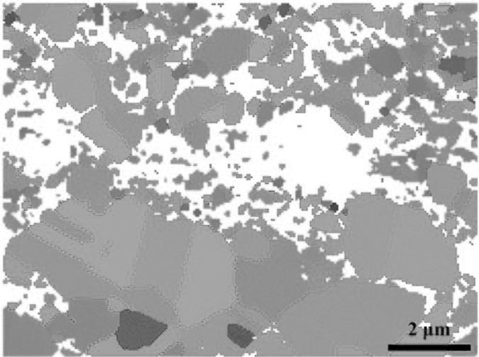
(a)

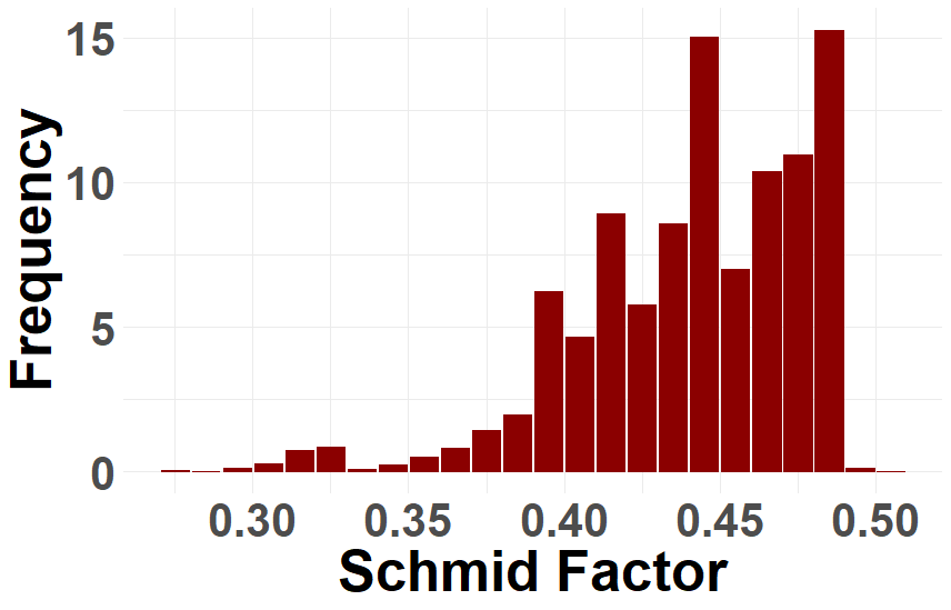
(b)

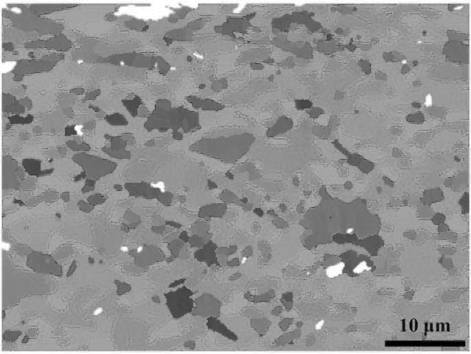
(c)

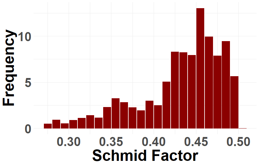
(d)

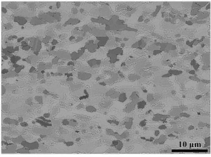
(e)

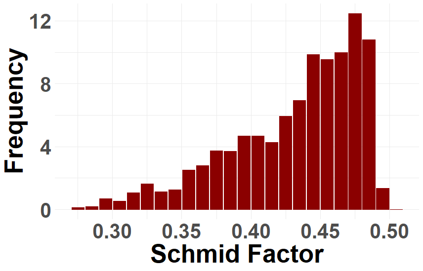
(f)

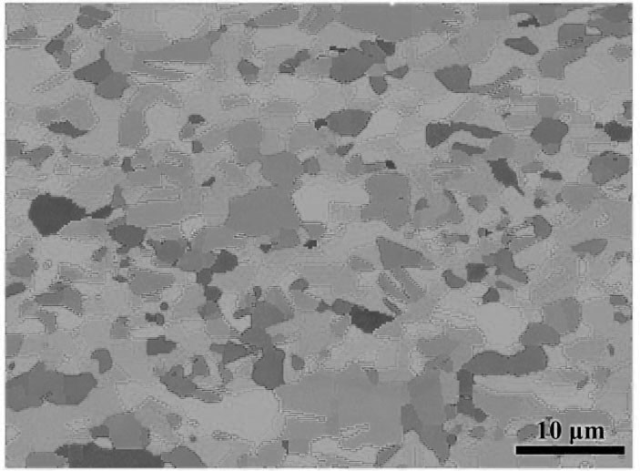
(g)

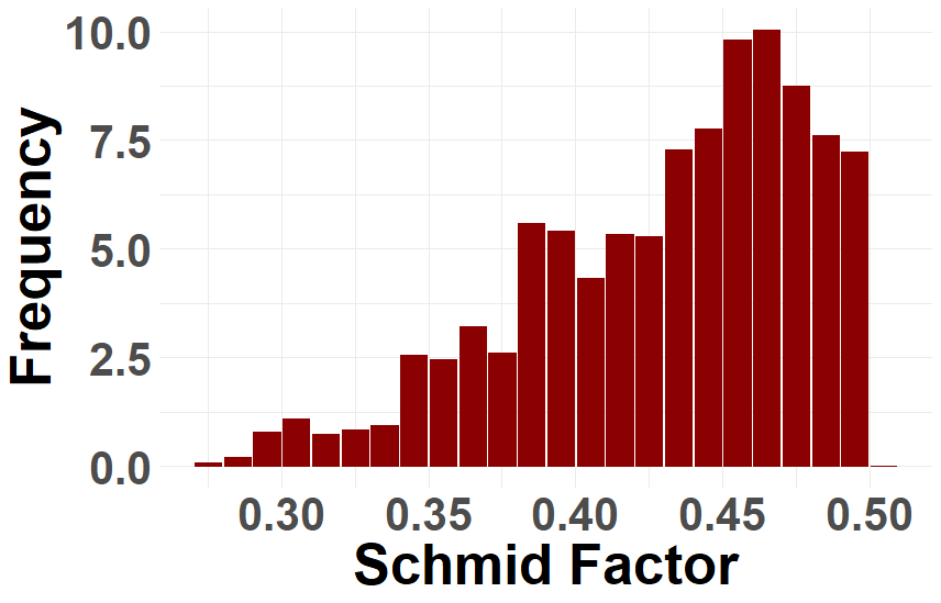
(h)

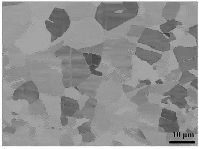
(i)

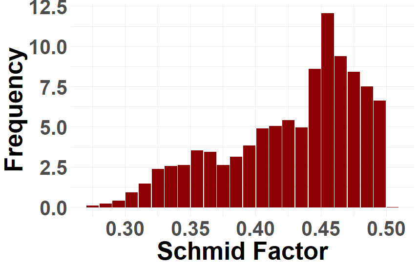
(j)

Figure 6: Schmid factor of AuSS annealed for 60 seconds at different temperatures. (a), (b): 700 ${}^{\circ}C$. (c), (d): 750 ${}^{\circ}C$. (e), (f): 800 ${}^{\circ}C$. (g), (h): 850 ${}^{\circ}C$. (i), (j): 950 ${}^{\circ}C$. The gray scale bar is associated with the range of values of the Schmid factor.

5.2 Data

The Schmid factor and its empirical distribution are obtained from an experiment performed on NG structured AuSS. The strips of such steels are cut and annealed at various temperatures ranging from 700 ${}^{\circ}C$ to 950 ${}^{\circ}C$. Figure 6 shows the distribution of Schmid factor for varying annealing temperatures. Light and dark gray regions represent lower and higher Schmid factor values, respectively. The authors of Na2021 have shown that steel strength and ductility improves when the annealing temperature ranges between 700-850 ${}^{\circ}C$, whereas steel strength decreases when the annealing temperature increases to 950 ${}^{\circ}C$. Indeed, the goal of this analysis is to reveal a similar behavior at temperatures 700-850 ${}^{\circ}C$ with the breaking point being at 950 ${}^{\circ}C$.

Table 1: $p-$values based on KS testing without RPDG, as described in Section 5.3. No statistically significant difference between associated temperatures is shown at the threshold 0.05.

	${750^{\circ}C}$	${800^{\circ}C}$	${850^{\circ}C}$	${950^{\circ}C}$
${700^{\circ}C}$	0.068	0.259	0.441	0.139
${750^{\circ}C}$		0.992	0.893	0.675
${800^{\circ}C}$			0.893	0.893
${850^{\circ}C}$				0.893

5.3 KS testing without RPDG

We have one histogram (empirical distribution) of the Schmid factor per annealing temperature, as shown in Figure 6 (right column). A two-sided Kolmogorov-Smirnov (KS) hypothesis test is performed for each pair of these empirical distributions of Schmid factors, and the associated $p$-values are reported in Table 1. It is noted that all of the $p-$values are higher than the significance level of $0.05$, thus indicating that the materials are showing similar behavior. This agrees with the experimental knowledge Na2021 for the annealing temperatures of 700${}^{\circ}C$, 750 ${}^{\circ}C$, 800 ${}^{\circ}C$ and 850 ${}^{\circ}C$, yet their behavior should have changed at the annealing temperature of 950 ${}^{\circ}C$. Thus, the KS hypothesis tests based on the empirical distributions of the Schmid factors for this experiment fail to uncover the important different behavior of materials at 950 ${}^{\circ}C$ as shown in Na2021 .

Table 2: $p-$values based on KS testing with RPDG, as described in Section 5.4. Bold indicates statistically significant difference between associated temperatures. The selected $p$-value threshold is $0.05$.

	${750^{\circ}C}$	${800^{\circ}C}$	${850^{\circ}C}$	${950^{\circ}C}$
${700^{\circ}C}$	0.063	0.002	0.123	0.002
${750^{\circ}C}$		0.572	0.791	$\mathbf{5.932\times 10^{-5}}$
${800^{\circ}C}$			0.123	$\mathbf{3.471\times 10^{-6}}$
${850^{\circ}C}$				$\mathbf{2.099\times 10^{-4}}$

5.4 KS testing with RPDG

Using the sublevel set filtration of Section 2.1.2, we generate five persistent diagrams (PDs) from the different empirical distributions of Schmid factors (based on the histograms in Figure 6) corresponding to the five different annealing temperatures. For each annealing temperature, we generate a sample of $100,000$ PDs using RPDG with an empirically chosen normal mixture as the proposal density. We then generate a histogram of persistence values for each set of $100,000$ PD samples, thereby obtaining five histograms. Subsequently, we perform a KS test for each pair of histograms and report the associated $p-$values in Table 2. Notice that aside from the pairing at annealing temperatures 700${}^{\circ}C$ and 800${}^{\circ}C$, all pairings agree with the experimental results Na2021 , and most importantly, our approach using RPDG reveals the different behavior at 950${}^{\circ}C$. Hence, the hypothesis test based on RPDG sampling can robustly establish a relationship between processing (annealing temperature), structure (distribution of the Schmid factor), and property (strength).

6 Conclusions

Data generation in experimental facilities may be expensive, and thus a small number of noisy data may be collected. Small sample size poses limitations to statistical analysis. To remedy this, we have proposed in this work random persistence diagram generation (RPDG), a method that randomly generates persistence diagrams (PDs) by retaining the topological properties encoded by the PD of a given dataset. An interesting theoretical direction is to examine if distributions of PDs generated by RPDG are stable under small perturbations of the initial PD, and in addition study rates of convergence in distribution.

RPDG makes two main contributions, a model of PDs based on a novel pairwise interacting point process and the first reversible jump MCMC (RJ-MCMC) technique for sampling PDs. It is typical for PDs to have a varying number of points, and RJ-MCMC accommodates the randomness in the location and number of points. The RPDG method currently treats parameter estimation in its PD model as a pre-processing step, e.g., the jump points in Definition 9 are empirically selected. A line of future research is to develop a Bayesian version of RPDG, which will account for uncertainty in its model parameters and will automatically estimate them.

Finally, we have employed our RPDG method to elicit from experimental data Na2021 the relationship of materials’ strength, as expressed by the Schmid factor, and annealing temperatures. As a matter of fact, our RPDG method matches the experimental knowledge, providing a modelling framework that enables the identification of changes in materials structure.

While RPDG has been applied to the aforementioned materials example in this paper, the main methodology is data-agnostic, and as such, it can find applications in a plethora of problems, including settings with small sample size, and data with imbalanced classes. To that end, synthetic data generation may be needed for statistical inference, and RPDG could be used for sampling synthetic topological summaries of data. For example, some healthcare applications involve two classes, a control and a treatment group; the treatment group may have a small sample size of pertinent images associated with a rare disease, and in turn RPDG could be utilized to counter this limitation by generating persistence diagrams that topologically summarize the shape of these images.

References

- \bibcommenthead
- (1) Edelsbrunner, H., Harer, J.L.: Computational Topology: an Introduction. American Mathematical Society, Providence, R.I. (2010)
- (2) Patrangenaru, V., Bubenik, P., Paige, R.L., Osborne, D.: Topological data analysis for object data. arXiv:1804.10255 (2018)
- (3) Guo, W., Manohar, K., Brunton, S.L., Banerjee, A.G.: Sparse-TDA: Sparse realization of topological data analysis for multi-way classification. IEEE Transactions on Knowledge and Data Engineering 30(7), 1403–1408 (2018)
- (4) Love, E.R., Filippenko, B., Maroulas, V., Carlsson, G.: Topological deep learning. arXiv:2101.05778 (2021)
- (5) Biscio, C.A.N., Møller, J.: The accumulated persistence function, a new useful functional summary statistic for topological data analysis, with a view to brain artery trees and spatial point process applications. Journal of Computational and Graphical Statistics, 1537–2715 (2019)
- (6) Nasrin, F., Oballe, C., Boothe, D.L., Maroulas, V.: Bayesian topological learning for brain state classification. In: Proceedings of 2019 IEEE International Conference on Machine Learning and Applications (ICMLA) (2019)
- (7) Maroulas, V., Mike, J.L., Oballe, C.: Nonparametric estimation of probability density functions of random persistence diagrams. Journal of Machine Learning Research 20(151), 1–49 (2019)
- (8) Khasawneh, F.A., Munch, E.: Chatter detection in turning using persistent homology. Mechanical Systems and Signal Processing 70–71, 527–541 (2016)
- (9) Marchese, A., Maroulas, V.: Signal classification with a point process distance on the space of persistence diagrams. Advances in Data Analysis and Classification 12(3), 657–682 (2018)
- (10) Maroulas, V., Nasrin, F., Oballe, C.: A Bayesian framework for persistent homology. SIAM Journal on Mathematics of Data Science 2(1), 48–74 (2020)
- (11) Townsend, J., Micucci, C.P., Hymel, J.H., Maroulas, V., Vogiatzis, K.D.: Representation of molecular structures with persistent homology for machine learning applications in chemistry. Nat Commun 11, 3230 (2020)
- (12) Humphreys, D.P., McGuirl, M.R., Miyagi, M., Blumberg, A.J.: Fast estimation of recombination rates using topological data analysis. GENETICS (2019)
- (13) Mileyko, Y., Mukherjee, S., Harer, J.: Probability measures on the space of persistence diagrams. Inverse Problems 27(12), 124007 (2011)
- (14) Munch, E., Turner, K., Bendich, P., Mukherjee, S., Mattingly, J., Harer, J.: Probabilistic fréchet means for time varying persistence diagrams. Electron. J. Statist. 9(1), 1173–1204 (2015)
- (15) Turner, K., Mileyko, Y., Mukherjee, S., Harer, J.: Fréchet means for distributions of persistence diagrams. Discrete and Computational Geometry 52(1), 44–70 (2014)
- (16) Bobrowski, O., Mukherjee, S., Taylor, J.E.: Topological consistency via kernel estimation. Bernoulli 23(1), 288–328 (2017)
- (17) Chazal, F., de Silva, V., Oudot, S.: Persistence stability for geometric complexes. Geometriae Dedicata 173(1), 193–214 (2014)
- (18) Blumberg, A.J., Gal, I., Mandell, M.A., Pancia., M.: Persistent homology for metric measure spaces, and robust statistics for hypothesis testing and confidence intervals. Found. Comput. Math. 4, 1–45 (2014)
- (19) Chazal, F., Fasy, B.T., Lecci, F., Rinaldo, A., Wasserman, L.: Stochastic convergence of persistence landscapes and silhouettes. In: Proceedings of the Thirtieth Annual Symposium on Computational Geometry, pp. 474–483 (2014)
- (20) Robinson, A., Turner, K.: Hypothesis testing for topological data analysis. Journal of Applied and Computational Topology 1(2), 241–261 (2017)
- (21) Fasy, B.T., Lecci, F., Rinaldo, A., Wasserman, L., Balakrishnan, S., Singh, A., et al.: Confidence sets for persistence diagrams. The Annals of Statistics 42(6), 2301–2339 (2014)
- (22) Chazal, F., Fasy, B., Lecci, F., Michel, B., Rinaldo, A., Rinaldo, A., Wasserman, L.: Robust topological inference: Distance to a measure and kernel distance. J. Mach. Learn. Res. 18(1), 5845–5884 (2017)
- (23) Adler, R.J., Agami, S., Pranav, P.: Modeling and replicating statistical topology and evidence for cmb nonhomogeneity. Proceedings of the National Academy of Sciences 114(45), 11878–11883 (2017)
- (24) Adler, R.J., Agami, S.: Modelling persistence diagrams with planar point processes, and revealing topology with bagplots. J Appl. and Comput. Topology 3, 139–183 (2019)
- (25) Baddeley, A., Turner, R.: Practical maximum pseudolikelihood for spatial point patterns. Australian & New Zealand Journal of Statistics 42(3), 283–322 (2000)
- (26) Okabe, A., Boots, B., Sugihara, K., Chiu, S.N.: Spatial Tessellations: Concepts and Applications of Voronoi Diagrams, 2nd ed. edn. Series in Probability and Statistics. John Wiley and Sons, Inc., New York, NY, USA (2000)
- (27) Strauss, D.J.: A model for clustering. Biometrika 62(2), 467–475 (1975)
- (28) Berman, M., Turner, T.R.: Approximating point process likelihoods with glim. Journal of the Royal Statistical Society. Series C (Applied Statistics) 41(1), 31–38 (1992)
- (29) Green, P.J.: Reversible jump markov chain monte carlo computation and bayesian model determination. Biometrika 82(4), 711–732 (1995)
- (30) Geyer, C.J., Moller, J.: Simulation procedures and likelihood inference for spatial point processes. Scand. J. Statist 21, 359–373 (1994)
- (31) Gong, N., Wu, H.-B., Yu, Z.-C., Niu, G., Zhang, D.: Studying mechanical properties and micro deformation of ultrafine-grained structures in austenitic stainless steel. Metals 7(6) (2017)
- (32) Murphy, W., Black, J., Hastings, G.: Handbook of Biomaterial Properties. Springer, New York, NY, USA (2016)
- (33) Li, J., Li, H., Liang, Y., Liu, P., Yang, L.: The microstructure and mechanical properties of multi-strand, composite welding-wire welded joints of high nitrogen austenitic stainless steel. Materials (Basel) 12(18), 2944 (2019)
- (34) Na, G., Farzana, N., Yong, W., Huibin, W., David, K., Vasileios, M., Orlando, R.: Persistent Homology on Electron Backscatter Diffraction Data in Nano/ultrafine-grained Metallic Materials (2021)