Universal Two-Component Dynamics in Supercritical Fluids

Abstract

Despite the technological importance of supercritical fluids, controversy remains about the details of their microscopic dynamics. In this work, we study four supercritical fluid systems—water, Si, Te, and Lennard-Jones fluid—via classical molecular dynamics simulations. A universal two-component behavior is observed in the intermolecular dynamics of these systems, and the changing ratio between the two components leads to a crossover from liquidlike to gaslike dynamics, most rapidly around the Widom line. We find evidence to connect the liquidlike component dominating at lower temperatures with intermolecular bonding, and the component prominent at higher temperatures with free-particle, gaslike dynamics. The ratio between the components can be used to describe important properties of the fluid, such as its self-diffusion coefficient, in the transition region. Our results provide insight into the fundamental mechanism controlling the dynamics of supercritical fluids, and highlight the role of spatiotemporally inhomogenous dynamics even in thermodynamic states where no large-scale fluctuations exist in the fluid.

1 Introduction

In the past few decades, supercritical fluids have attracted renewed interest due to their applications in a wide range of chemical and materials processing industries ¹. Most interesting applications of supercritical fluids fall in the region close to the critical point ^{1, 2}. There, the fluids exhibit unique properties combining the advantages of liquids (e.g., high densities) and gases (e.g., high diffusivities), and these properties are highly tunable with relatively small changes in temperature, $T$, and pressure, $P$ ². Thus, it is important to understand these properties and their dependence on the thermodynamic state.

Thanks to many years of research, the thermodynamics of supercritical fluids, which is based on their macroscopic properties, has become well understood. In particular, the concept of the Widom line has been introduced to refer to the line of maxima of a given response function, such as the isobaric heat capacity, $C_{P}$ ³. Although not a rigorous separatrix between liquid and gas states ⁴, the Widom line indicates rapid changes in the thermodynamic properties of supercritical fluids, especially in the near-critical region. Around the Widom line, a crossover between liquidlike and gaslike properties is expected for the fluid ⁵.

The picture is less clear when it comes to molecular-scale dynamics of supercritical fluids, which should reveal the microscopic mechanism behind many of the macroscopic properties. One of the first systematic studies on this topic was done by Simeoni et al. ⁶. Using classical molecular dynamics (MD) simulations supported by inelastic x-ray scattering (IXS) data, they observed a crossover in the deep supercritical region along an extension of the Widom line.

Our previous work ⁷ focused instead at a region close to the critical point, where the Widom line is very clear. We used both IXS measurements and MD simulations to study the intermolecular dynamics of supercritical water in the region $0.9<P/P_{c}<2.3$, $0.6<T/T_{c}<1.2$, where $P_{c}$ and $T_{c}$ are the critical pressure and temperature. Contrary to previous approaches ^{6, 8}, we found that the intermolecular dynamics at a given $P,T$ state cannot be consistently described using models developed for liquids, but instead can be decomposed into two components—a high-frequency component associated with the stretching mode between hydrogen-bonded molecules, and a low-frequency component representing free-particle motions. With changing thermodynamic states, it is the ratio between the two components that changes, with a rapid crossover observed near the Widom line. However, remnants of both components can be found on either side of the Widom line.

It is natural to ask whether the observed two-component dynamics is specific to water, whose liquidlike dynamics arises from hydrogen bonds, or can be generalized to other supercritical fluids. In this work, we aim at answering this question by studying the potentials representing four different supercritical fluid systems—water, Si, Te, and Lennard-Jones (LJ) fluid—via classical MD simulations. Even though these systems have very different interatomic potentials (see the Methods section below), the two-component behavior is universal in their molecular dynamics. Moreover, we find evidence to associate the liquidlike component with the degree of intermolecular bonding, and the gaslike component with dynamics similar to that in an unbonded, free gas state. As in the case of water, a fast change in the ratio between the two components marks the dynamical crossover, but both components exist on either side of the transition. The fraction of the components can also be used to describe transport properties of the fluid, such as its self-diffusion coefficient.

2 Methods

2.1 Simulation details

In this study, we investigate four fluid systems with different potential models:

1. Water, with the TIP4P/2005 potential ⁹. This potential includes a Lennard-Jones (LJ) interaction between oxygen sites and long-range Coulomb force between all charged sites.

2. Si, with the Stillinger-Weber (SW) potential ¹⁰. This potential include pairwise interactions as well as three-body interactions, both short-ranged (cut off at $3.771\text{\,}\mathrm{\SIUnitSymbolAngstrom}$). The three-body interaction term favors local tetrahedral ordering.

3. Te, with an analytical bond-order potential (BOP) ¹¹. This potential considers the effect of bond orders, which are functions of the local environments of the atoms, on the bond energy.

4. LJ fluid, with the shifted-force (sf) potential:

   $$u^{\mathrm{sf}}(r)=\begin{cases}u(r)-u(R_{c})-(r-R_{c})\left.\frac{du(r)}{dr}\right|_{r=R_{c}},&\text{if $r<R_{c}$}\\ 0,&\text{if $r\geq R_{c}$}\end{cases}$$ (1)

   where $r$ is the distance between interacting atoms, $R_{c}$ is the cutoff distance, and

   $$u(r)=4\epsilon\left[\left(\frac{\sigma}{r}\right)^{12}-\left(\frac{\sigma}{r}\right)^{6}\right]\\$$ (2)

   is the standard 12-6 potential. $\epsilon$ and $\sigma$ are energy and distance units, respectively. Other units for the LJ fluid can be expressed in terms of $\epsilon$, $\sigma$, and the atomic mass $M$. For example, the units for time is $\tau\equiv\sqrt{M\sigma^{2}/\epsilon}$. In this work, we set $R_{c}=2.5\sigma$.

The MD simulations are carried out using the LAMMPS simulation package ¹². The simulation box contains $2880$ molecules for water and $4000$ atoms for Si, Te, and LJ fluid. We use $NPT$ ensembles, with a Nosé-Hoover thermostat and barostat. The damping constants are $1\text{\,}\mathrm{p}\mathrm{s}$ for water, Si, and Te, and $1\tau$ for LJ. After equilibration at each $P,T$ state, the simulation is run for $1\text{\,}\mathrm{n}\mathrm{s}$ (with $1\text{\,}\mathrm{f}\mathrm{s}$ time steps) for water, $0.4\text{\,}\mathrm{n}\mathrm{s}$ (with $1\text{\,}\mathrm{f}\mathrm{s}$ time steps) for Si, $1\text{\,}\mathrm{n}\mathrm{s}$ (with $2.5\text{\,}\mathrm{f}\mathrm{s}$ time steps) for Te, and $1000\tau$ (with $0.001\tau$ time steps) for LJ.

2.2 Critical parameters

Table 1 presents the critical point parameters for the fluid systems in this study. The TIP4P/2005 model for water, the SW model for Si, and the LJ fluid model are well-studied and their critical parameters can be found in the literature. The critical point parameter for the BOP Te model is determined using a direct MD simulation method ¹³; more details are provided in the Supporting Information. Most of the results below focus on the temperature dependence of the properties of the fluid along an isobar $P\approx 1.6P_{c}$; the exact value of $P$ for each system is listed in the last column in Table 1. Figure 1 shows the (reduced) $P$-$T$ phase diagram of all the systems, as well as the thermodynamic states simulated in this study. We note that, as mentioned in the Discussion section below, the two-component phenomenon is not an anomaly arising from large-scale critical fluctuations, and the isobars taken are sufficiently away from the critical point. Therefore, the results in this study are robust against errors in the critical point parameters.

Table 1: Critical point parameters for the models used in this study and the isobar pressure $P$. The units for water, Si, and Te are: $T_{c}$ in $\mathrm{K}$, $P_{c}$ and $P$ in $\mathrm{b}\mathrm{a}\mathrm{r}$, and $\rho_{c}$ in $\mathrm{g}\mathrm{/}\mathrm{{}^{3}}\mathrm{c}\mathrm{m}$. The last column shows the temperature range investigated for each system.

Model	$T_{c}$	$P_{c}$	$\rho_{c}$	$P$	$T$ range
water 14	$640\pm 16$	$146\pm 7$	$0.337\pm 0.008$	225	546 to 846
Si 15	$7925\pm 250$	$1850\pm 400$	$0.75\pm 0.10$	2850	5200 to 11200
Te	$2080\pm 40$	$530\pm 40$	$2.17\pm 0.04$	870	1160 to 2760
LJ 16	$0.937\epsilon/k_{B}$	$0.0820\epsilon/\sigma^{3}$	$0.320\sigma^{-3}$	$0.13\epsilon/\sigma^{3}$	0.7 to $1.3\,\epsilon/k_{B}$

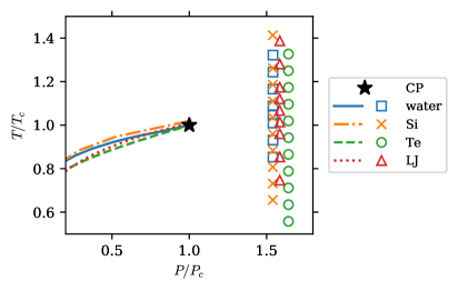
Figure 1: $P$-$T$ phase diagram of the systems in reduced units. The lines show the liquid-vapor coexistence line for the systems (see Refs. 17, 18, 16 for water, Si, and LJ, and Supporting Information for Te), which terminate at the critical point (CP, black star). The symbols show the thermodynamic states included in this study.

3 Results

3.1 Two-component dynamics

The molecular dynamics of fluids is usually described by the dynamic structure factor, $S(Q,\omega)$, which measures the correlation of density fluctuations in wavenumber ($Q$) and frequency ($\omega$) space ¹⁹. It is defined as

$$S(Q,\omega)=\frac{1}{2\pi}\int_{-\infty}^{\infty}dt\;e^{-i\omega t}\left<\rho_{Q}^{*}(0)\rho_{Q}(t)\right>,$$ (3)

where angular brackets indicate the ensemble average, and $\rho_{Q}(t)=\sum_{n=1}^{N}e^{i{\bf Q}\cdot{\bf r}_{n}(t)}\left/\sqrt{N}\right.$ is the density in $Q$-space at time $t$, ${\bf r}_{n}(t)$ being the position of the $n^{\text{th}}$ atom. In this paper, we take the classical limit. $S(Q,\omega)$ is one of the most important functions to describe the molecular dynamics of fluids, as it contains all the relevant information on the dynamics of the system ¹⁹. Moreover, at wavenumbers approaching intermolecular scales ($Q\sim${\mathrm{\SIUnitSymbolAngstrom}}^{-1}$$), $S(Q,\omega)$ can be directly measured using inelastic neutron and x-ray scattering ^{19, 20}.

The dynamics in different thermodynamic states can be conveniently compared using the longitudinal current correlation $J(Q,\omega)$, defined by replacing the density $\rho_{Q}(t)$ in Eq. (3) with the longitudinal current $j_{Q,l}(t)=\sum_{n=1}^{N}v_{n,l}(t)e^{i{\bf Q}\cdot{\bf r}_{n}(t)}\left/\sqrt{N}\right.$. Here, $v_{n,l}(t)$ denotes the velocity of the $n^{\text{th}}$ atom along the direction of ${\bf Q}$. It bears a simple relation to $S(Q,\omega)$ ¹⁹:

$$J_{l}(Q,\omega)=\frac{\omega^{2}}{Q^{2}}S(Q,\omega).$$ (4)

$J(Q,\omega)$ obeys the classical sum rule ¹⁹:

$$\frac{M}{k_{B}T}\int_{-\infty}^{\infty}J_{l}(Q,\omega)d\omega=1,$$ (5)

where the pre-factor contains only the molecular mass $M$, the Boltzmann constant $k_{B}$, and the temperature $T$, all of which are known constants for the simulation. This provides a simple way to normalize and compare the spectra for different thermodynamic states.

With the help of this normalization, the two-component behavior in the fluid systems becomes clear. This can be seen in Fig. 2, where the symbols on the left column show the normalized spectra, $J_{l}(Q,\omega)\times(M/k_{B}T)$, obtained from MD simulations. Each row presents one of the four fluid systems in this study—water, Si, Te, and LJ fluid—as indicated. For each system, three temperature points are taken along an isobar of $P\approx 1.6P_{c}$ as indicated in Table 1: a low-temperature state (blue circles), an intermediate temperature state (grey squares), and a high-temperature state (red triangles). The $Q$ value is chosen to be approximately $0.5Q_{m}$, where $Q_{m}$ is the position of first peak in the structure factor $S(Q)$; in real space, this $Q$ corresponds to approximately twice the average intermolecular distance. We note that the same two-component phenomenon can be observed at other $Q$ values at least in the range from $0.3Q_{m}$ to $0.8Q_{m}$, as was also the case in our previous work ⁷.

The black lines in Fig. 2 show the spectra expected of the gas state. For water, Si, and LJ fluid, this is taken to be the free-particle limit, assuming simply a Maxwell-Boltzmann velocity distribution with no interaction ^{19, 7}:

$$J_{l}^{\text{free}}(Q,\omega)=\frac{\omega^{2}}{\sqrt{2\pi}Q^{3}v_{0}}\exp\left[-\frac{1}{2}\left(\frac{\omega}{Qv_{0}}\right)^{2}\right],$$ (6)

where $v_{0}\equiv\sqrt{k_{B}T/M}$ is the thermal velocity. The temperature is taken to be the same as the high-$T$ state, although small changes in $T$ lead only to a slight shift ($\propto\sqrt{T}$) in the peak position and do not appear to significantly influence the results below. For Te, the gas phase is diatomic (i.e., it consists of Te₂ dimers), so there is an additional peak around $23\text{\,}\mathrm{m}\mathrm{e}\mathrm{V}$ corresponding to the dimer stretching mode (see Supporting Information for more details). Hence, a simple expression cannot be obtained for $J_{l}^{\text{free}}(Q,\omega)$, and we use instead a low-$P$ spectrum at $100\text{\,}\mathrm{b}\mathrm{a}\mathrm{r}$, $2760\text{\,}\mathrm{K}$, where the density is only $0.109\text{\,}\mathrm{g}\mathrm{/}\mathrm{{}^{3}}\mathrm{c}\mathrm{m}$ compared to the critical density of $2.17\text{\,}\mathrm{g}\mathrm{/}\mathrm{{}^{3}}\mathrm{c}\mathrm{m}$. It can be seen that the high-$T$ spectrum is close to the gas state for all systems.

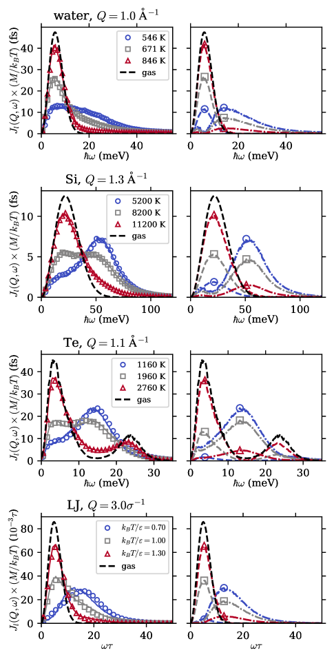
Figure 2: Two-component behavior in the longitudinal current correlation function. Each row shows a different fluid system. The left columns show data from simulation (symbols) along with the NMF fit (solid lines). For each system we choose three states along an isobar $P\approx 1.6P_{c}$: a low-temperature, liquidlike state (blue circles), an intermediate state in the crossover region (grey squares), and a high-temperature, gaslike state (red triangles). The right column shows the L component (dash-dotted lines) and G component (dashed lines) obtained from NMF, and the peak positions are marked by corresponding symbols. For reference, we show in both columns the gas limit as black dashed lines without symbols. $\sigma$ and $\epsilon$ are LJ units.

From these plots it is clear, particularly for Si and Te, that the intermediate state contains features of both the low and the high temperature spectra as in the case of water ⁷. Specifically, the intermediate spectrum in Si shows both the peak around $55\text{\,}\mathrm{m}\mathrm{e}\mathrm{V}$ which is prominent in the low-$T$ state and the peak around $20\text{\,}\mathrm{m}\mathrm{e}\mathrm{V}$ which dominates the high-$T$ state, and similarly for Te (including the dimer oscillation peak around $23\text{\,}\mathrm{m}\mathrm{e}\mathrm{V}$). In the case of the LJ fluid, even though we do not observe two distinct peaks, the intermediate temperature spectrum can still be interpreted as a linear combination of the high and low temperature states. In addition, as will be shown below, this interpretation can be used to predict other properties of the LJ fluid in the same way as for the other systems. Therefore, our results show that there is a universal two-component behavior in the supercritical fluids under study.

3.2 NMF analysis and the liquidlike to gaslike transition

In order to describe the spectra quantitatively, a method is needed to extract the two components. To our knowledge, however, no existing theory can adequately describe the two-component phenomenon and provide a model to fit the data. Therefore, we adopt the nonnegative matrix factorization (NMF) method ²¹ used in our previous study ⁷, which provides a model-free way to extract the components in the spectra. Mathematically, we optimize the decomposition

$$\frac{M}{k_{B}T}J_{l}(Q,\omega;P,T)=c_{\text{L}}(P,T)J_{l}^{\text{L}}(Q,\omega)+c_{\text{G}}(P,T)J_{l}^{\text{G}}(Q,\omega)$$ (7)

where $J_{l}^{\text{L}}(Q,\omega)$ and $J_{l}^{\text{G}}(Q,\omega)$ are the L and G components dominating in the liquidlike (low $T$) and gaslike (high $T$) states, respectively; the shapes of these components are assumed to be independent of $P$ and $T$. The pressure and temperature-dependence of the normalized spectra are captured entirely in the coefficients $c_{\text{L}}(P,T)$ and $c_{\text{G}}(P,T)$. When fitting, we include all temperatures along the isobar and add the gas state as well. It also turns out that spectra from different $Q$ can be fit together, resulting in the same coefficients $c_{\text{L}}(P,T)$ and $c_{\text{G}}(P,T)$. Because we are interested in molecular-scale dynamics, in this work we typically use data from $0.3Q_{m}$ to $0.8Q_{m}$, which corresponds to length scales on the same order as the average intermolecular distance. Small changes in the $Q$ range used for fitting do not have a significant influence on the results below. When $Q<0.3Q_{m}$, the data tend to be noisier because of the finite system size and energy resolution.

Results of the NMF decomposition are shown in Fig. 2. On the left column, the solid lines show the NMF fit (sum of the components), which agrees well with data (symbols); on the right column, the G and L components are shown as dashed and dash-dotted lines, respectively, with the corresponding symbols indicating their respective peak positions. In all systems, the G component is close in shape to the gas state spectrum, and the L component peaks at a higher frequency. With increasing temperature, the spectral weight shifts from the L to the G component, leading to a liquidlike to gaslike transition.

Because of the sum rule, Eq. (5), we normalize the L and G components as well so that $\int_{-\infty}^{\infty}J_{l}^{\text{L,G}}(Q,\omega)d\omega=1$. As a result, $c_{\text{L}}+c_{\text{G}}=1$, so we may interpret $c_{\text{L}}$ and $c_{\text{G}}$ as the fraction of the L and G components. If we now define the parameter $f\equiv c_{\text{L}}$, it can be seen from Eq. (7) that the spectral evolution is captured entirely by the single parameter $f$ as a function $P$ and $T$, and any dynamical crossover on an isobar should show up when plotting $f(T)$.

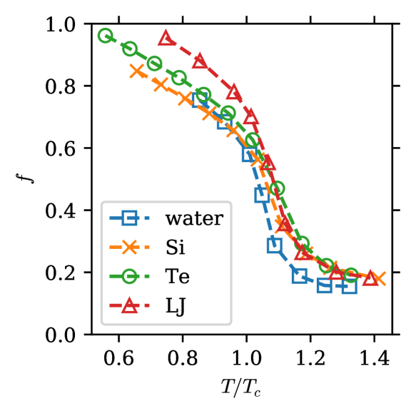
Figure 3: Dependence of the fraction of the L component, $f$, on reduced temperature $T/T_{c}$ along the isobar $P\approx 1.6P_{c}$. Blue squares: water; yellow crosses: Si; green circles: Te; red triangles: LJ fluid. Dashed lines are a guide to the eye.

Therefore, in Fig. 3 we present $f$ as a function of reduced temperature $T/T_{c}$ for all four systems. The overall shape and value of the curves are very similar for all the systems. This is consistent with van der Waals’s law of corresponding states ²² and provides evidence for the universality of the two-component behavior among supercritical fluids. In particular, all curves show an “S” shape with a rapid decrease slightly above $T/T_{c}=1$. The position of the fast change in $f$ agrees well with the expected location of the Widom line. To show this, we plot in Fig. 4 the enthalpy, $H$, against the parameter $f$. The former can be easily obtained from MD simulations. An approximately linear relation can be seen between $f$ and $H$ for all systems, with linear fits shown as solid lines. Because the isobaric heat capacity, $C_{P}$, is the derivative of $H$ with respect to temperature along the isobar, the linearity between $f$ and $H$ implies that $|df/dT|$ peaks at roughly the same temperature as $C_{P}$, i.e., near the Widom line. In other words, the dynamics change most rapidly around the Widom line. We note that although the Widom line here has a specific definition ($C_{P}$ maximum along an isobar), in the near-critical region it is expected to lie close to the Widom lines obtained by other definitions as well. For example, in the case of water, it has been shown that the rapid changes in $f$ are close to the Widom lines with several different definitions ⁷.

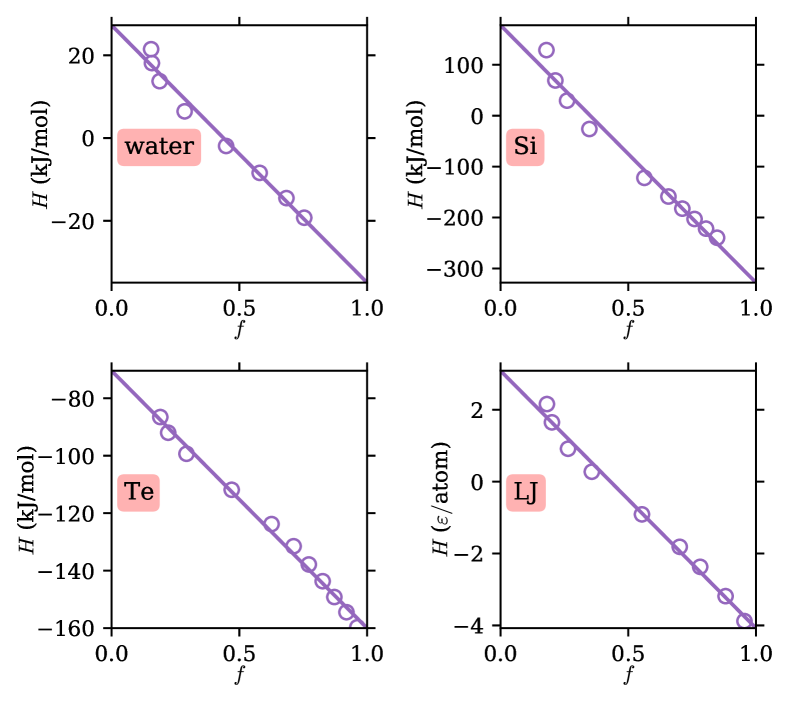
Figure 4: Relation between the enthalpy, $H$, and the parameter $f$. Data are shown as empty circles, and the linear fits as solid lines. $\epsilon$ is the LJ energy unit (see Method).

3.3 The L component and intermolecular bonding

Having established above that the G component corresponds to the gas state, we now turn to the physical origin of the L component. In the case of water, our previous work ⁷ has provided evidence that this component is related to the O—O stretching motion between hydrogen-bonded molecules. Therefore, it is reasonable to hypothesize that the L component in the other systems is related to intermolecular bonding as well.

To investigate this, it is necessary to define “bonding” for these systems. Because the LJ fluid has only a pairwise interaction that depends solely on the interatomic distance, it is natural to define a cutoff distance $R_{b}$ below which a pair is considered bonded. In the following, we take $R_{b}=1.6\sigma$, close to the first minimum in the radial distribution function $g(r)$ in the low-temperature state at $T=0.7\epsilon/k_{B}$, $P=0.13\epsilon/\sigma^{3}$ (see Supporting Information for details on $g(r)$).

The cases of Si and Te are in principle more complicated. Unlike water, whose hydrogen bonds can be defined by the geometry and/or the interaction energy between two molecules, Si and Te contain interactions terms that involve three or more atoms (see the Methods section). To our knowledge, there is no established way to define “bonding” in these systems. Hence, we simply define two atoms to be bonded if they are closer than a cutoff distance $R_{b}$. As in the case of the LJ fluid, $R_{b}$ is chosen to be around the first minimum in the radial distribution function for the low-temperature state, which is about $3.5\text{\,}\mathrm{\SIUnitSymbolAngstrom}$ and $4.2\text{\,}\mathrm{\SIUnitSymbolAngstrom}$ for Si and Te, respectively (see Supporting Information).

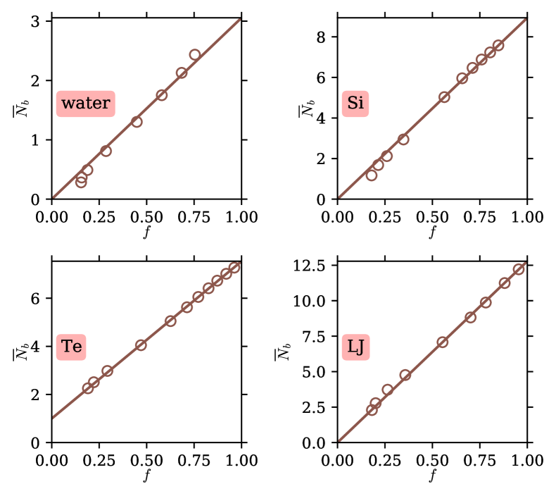
Figure 5: Relation between the number of bonds per atom (or water molecule), $\overline{N}_{b}$, and the parameter $f$. Data are shown as empty circles. For water, Si, and LJ, the data are consistent with an intercept of $\overline{N}_{b}=0$ at $f=0$, as the solid lines show. For Te, the data are consistent with an intercept of $\overline{N}_{b}=1$ at $f=0$ shown by the solid line.

In Fig. 5, the circles show the average number of bonds each atom (or water molecule) has, $\overline{N}_{b}$, plotted against the parameter $f$. For water, as in our previous work, we use a common definition for hydrogen bonding: two molecules are hydrogen-bonded if their O–O distance is less than $3.5\text{\,}\mathrm{\SIUnitSymbolAngstrom}$ and the O$\cdots$O—H angle is less than $30\mathrm{°}$ ^{23, 24}. For Si, Te, and LJ, we use the cutoff distance definition mentioned above. The data show very good linearity between $\overline{N}_{b}$ and $f$. Moreover, for water, Si, and LJ, the data are consistent with a zero intercept at $f=0$, as the solid lines show. For Te, as mentioned above and shown in more details in the Supporting Information, the gas state consists of Te₂ dimers, so we expect each atom to have exactly one bond. Indeed, the data are consistent with an intercept of $\overline{N}_{b}=1$ at $f=0$, as the solid line shows. These results strongly support that the L component, which dominates in low-temperature, liquidlike states, is directly related to intermolecular bonding for all systems studied. In the gas state, little to no bonding remains, and the L component disappears. We note that for water, using other hydrogen bonding definitions with various levels of strictness does not alter the conclusion, and for Si, Te, and LJ, the conclusion is robust against changes in the cutoff distance being used up to at least 10% (see Supporting Information).

3.4 Application: modeling the self-diffusion coefficient

Our results above have provided evidence for the two-component dynamical behavior and have shown that $f$ is a descriptor for the microscopic dynamics in the liquidlike to gaslike crossover. Since the microscopic dynamics is closely related to macroscopic transport properties , there should be a close relation between $f$ and transport properties as well. Below we show one such example.

One of the most important transport properties for supercritical fluids, especially for industrial applications, is the self-diffusion coefficient, $D$. This quantity can be easily obtained from MD simulations using the mean squared displacement ¹⁹:

$$D=\frac{1}{6}\lim_{t\to\infty}\frac{\left<|{\bf r}(t)-{\bf r}(0)|^{2}\right>}{t},$$ (8)

where ${\bf r}(t)$ the position of a given particle at time $t$. Here angular brackets denote the ensemble average. For water, we use the position of the O atom. The simulation times are long enough to reach the $t\to\infty$ limit. Alternatively, $D$ can be obtained using the velocity autocorrelation function ¹⁹:

$$D=\frac{1}{3}\int_{0}^{\infty}\left<{\bf v}(0)\cdot{\bf v}(t)\right>dt,$$ (9)

where ${\bf v}(t)$ is the velocity of a given particle at time $t$. The results from the two methods agree within 5%.

Earlier work ⁵ found that the self-diffusion coefficient for supercritical water appeared to follow an Arrhenius equation in the liquidlike and the gaslike region along each isobar. A dynamical crossover was found in between, but no specific model was given to describe it. Here we propose a model in which the parameter $f$ is used to describe this transition.

A good model should reduce to the observed dependence in the gaslike and liquidlike limits. In the limit of a dilute gas, it is well known ^{25, 26} that $D$ has a power-law dependence on either the temperature $T$ or the density $\rho$ ($T$ and $\rho$ are inversely related on an isobar by the ideal gas law). Since in this limit the density should be proportional to the number of bonds per atom, which is in turn proportional to $f$, we expect $D$ to have a power-law dependence on $f$ as well. In the dense liquid limit, $D$ is often described instead by the free volume model ^{27, 28}: $D\propto\exp(-A_{v}/V_{f})$, where $A_{v}$ is a constant and $V_{f}$ the free molecular volume (i.e., the average volume per molecule in excess of its Van der Waals volume). Under the framework of our two-component dynamics description, we draw an analogy between the free volume, $V_{f}$, and the fraction of the gaslike component, $1-f$. This can be justified by noting that, as shown above, the gaslike dynamic component corresponds to free-particle-like diffusive motions in the fluid. Therefore, in the dense liquid limit, we expect $D\propto e^{-A/(1-f)}$ where $A$ is a constant.

Combining the two limits, we build the following model for the self-diffusion coefficient:

$$D=D_{0}f^{-n}\exp\left(-\frac{A}{1-f}\right),$$ (10)

where $D_{0}$, $n$, $A$ are constants. In the gaslike limit, $f\to 0$, so $D\to D_{0}f^{-n}e^{-A}\propto f^{-n}$, i.e. it shows the expected power-law dependence. In the liquidlike limit, $f\to 1$, so $D\to D_{0}e^{-A/(1-f)}$ in line with the discussion above. We use Eq. (10) to fit the data with $D_{0}$, $n$, and $A$ as fit parameters, and the results are shown in Fig. 6. The model is able to fit the data well, including the crossover region near the Widom line where $D$ increases rapidly with temperature. Values of the fit parameters are shown in Table 2. Except for Te, the exponent $n$ in the gas limit is similar to literature values: $n=1.5$ from the Chapman-Enskog theory ²⁶, and $n=1.823$ for nonpolar systems according to Slattery and Bird’s fit for experimental data ²⁵. Note that, as mentioned above, on an isobar we expect $f\propto\rho\propto T^{-1}$, so we can rewrite expressions in the literature in terms of $f$. Through this example, we show that $f$ can be used to describe macroscopic transport properties across the liquidlike to gaslike transition, connecting the limits of a dense liquid and a dilute gas. Given the proportionality between $f$ and the number of bonds, $\overline{N}_{b}$, Eq. (10) may also be rewritten in terms of $\overline{N}_{b}$ and expanded to cover a wider range of thermodynamic states. This can be grounds for future investigations.

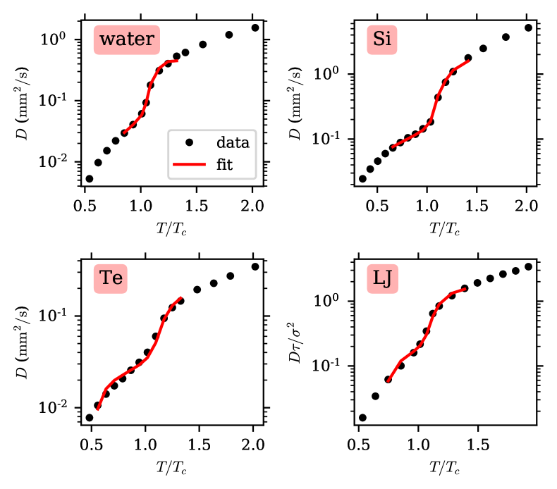
Figure 6: The self-diffusion coefficient, $D$, plotted against reduced temperature along an isobar $P\approx 1.6P_{c}$. The MD data are shown as black dots. The red lines show the fits using Eq. (10) over the range where $f$ is available through the two-component analysis.

Table 2: Fit parameters for the self-diffision coefficient model, Eq. (10). $D_{0}$ is in units of $\mathrm{m}\mathrm{m}\mathrm{{}^{2}}\mathrm{/}\mathrm{s}$ (for water, Si, Te) or $\sigma^{2}/\tau$ (for LJ).

System	$\ln D_{0}$	$n$	$A$
water	$-3.16\pm 0.28$	$1.38\pm 0.12$	$0.181\pm 0.075$
Si	$-2.66\pm 0.11$	$1.84\pm 0.07$	$0.034\pm 0.021$
Te	$-3.83\pm 0.08$	$1.22\pm 0.08$	$0.033\pm 0.006$
LJ	$-1.93\pm 0.10$	$1.42\pm 0.08$	$0.044\pm 0.008$

4 Discussion & Conclusions

In order to demonstrate the universality of the two-component phenomenon, we have chosen in our study four systems containing very different interatomic interactions (see the Methods section for more details)—the simple pairwise LJ potential, TIP4P/2005 water ⁹ with long-range Coulomb forces, Stillinger-Weber (SW) silicon ¹⁰ with a three-body term favoring local tetrahedral coordination, and tellurium bond-order potential ¹¹ where the gas phase is diatomic. The appearance of the two-component dynamics in all systems shows that this phenomenon is not specific to the local bonding mechanism, but common among several supercritical fluid systems. Consequently, any theory describing the molecular-scale dynamics of supercritical fluids, particularly the crossover between liquidlike and gaslike behavior, should take into account the existence of at least two components in the dynamics.

We note that the two-component phenomenon is not an anomaly arising from large-scale critical fluctuations, since the thermodynamic states in this study are sufficiently far away from the critical point and no such large-scale fluctuations are observed in our simulations. Instead, our results suggest the presence of spatiotemporally heterogeneous dynamics on the molecular scale, reflecting unbounded and bounded particle motions. Notably, a recent work ²⁹ using machine learning on local structural information has also found the existence of molecular-scale heterogeneities in supercritical LJ fluids. Because of this, the two-component phenomenon is not expected to appear in the long wavelength (low $Q$) limit. This has not been explored in our study by the low $Q$ cutoff around $0.3Q_{m}$ as mentioned in the Results section. Nonetheless, macroscopic quantities are influenced by their microscopic mechanisms and, as shown above, the use of the two-component model for the molecular dynamics can help build a more fundamental understanding of macroscopic properties such as the diffusion coefficient.

We mention here another dynamical crossover proposed in the literature, the “Frenkel line”, which separates the supercritical region into “rigid” and “non-rigid” fluids depending on the relaxation time of the system ³⁰. The underlying assumption there is that a single relaxation time describes the dynamics of all the fluid. Here we have shown, at least in the near-critical region we have investigated, that the dynamics is spatiotemporally heterogeneous. Thus it is not appropriate to describe the dynamics as purely liquid-like or gas-like, but rather a combination of both. In our previous work on supercritical water ⁷ including both experimental and simulation results, no significant change was observed near the proposed Frenkel line position. However, we have not investigated the deep supercritical region where the Frenkel line might also exist ³⁰; this may be a subject for future studies.

A limitation of our methodology using the NMF decomposition is the assumption that the shapes of the components do not change with the thermodynamic state. This of course does not work at all temperatures and pressures; for example, going to extremely high temperatures, the free-particle limit will be broadened according to Eq. (6). However, the fact that the NMF fit shown in Fig. 2 works well indicates that this assumption is valid over the temperature range under study, around $0.6T_{c}$ to $1.4T_{c}$. As mentioned in the introduction, this range around the critical point is the most interesting for applications. A more rigorous theory taking into account the change in the shape of the components may be able to describe a wider range of thermodynamic conditions.

We emphasize that one interesting point of our approach is that it can be checked against scattering experiments, for example high-resolution inelastic X-ray scattering ²⁰. These experiments directly measure the dynamical structure factor, $S(Q,\omega)$ ^{19, 20}, and the simple relation given by Eq. (4) connects it to $J_{l}(Q,\omega)$. The $J_{l}(Q,\omega)$ spectra are all that is needed for the two-component analysis and the extraction of the parameter $f$. Thus, $f$ is a descriptor of microscopic dynamics that is experimentally accessible and, as shown above, it is connected with various other properties of the fluid. In our previous work ⁷, we have indeed used inelastic X-ray scattering to measure the molecular dynamics of supercritical water, and found excellent agreement between experimental data and MD simulation results. Similar measurements can be done on other supercritical fluid systems as well to verify experimentally the universality of the two-component phenomenon found in this study. We note that, while the TIP4P/2005 water potential and the LJ potential have been shown to reproduce well experimental data on the dynamics of supercritical water ⁷ and argon ³¹, the Si and Te potentials used in this study have not been optimized or checked against experimental data in the supercritical region, since no data is yet available.

This universality and the close relation between intermolecular bonding and the L component is reminiscent of the well-known lattice gas model ^{32, 33}, which forms the basis connecting the liquid-gas critical point to the 3D Ising universality class. In the lattice gas model, a liquid-to-gas transition takes place with the breaking of bonds, which is similar to the behavior of $f$ and its connection to intermolecular bonding found in our study. Furthermore, we note that both in the lattice gas model and in our two-component analysis the transition from liquidlike to gaslike happens gradually with a continuous loss of bonds. Therefore, our study suggests that the understanding of supercritical fluids based on the lattice gas model may be extended into the description of their molecular dynamics as well.

In conclusion, our results show that the two-component phenomenon in the molecular dynamics, previously observed in supercritical water ⁷, is universal among several supercritical fluid systems with different intermolecular interactions. While the gaslike (G) component corresponds to free-particle motion in a dilute gas, the liquidlike (L) component can be associated with intermolecular bonding (a generalization of hydrogen-bonding in the case of water). These observations are shown to have important implications for transport properties such as the self-diffusion coefficient, particularly in bridging the liquidlike to gaslike transition, which is relevant to industrial applications.

Supporting Information.

Details on: i) the dimer gas phase of the Te BOP potential, ii) simulation results to determine the critical parameters of the Te BOP potential, iii) the components retrieved by NMF fit and the dispersion relation, iv) hydrogen bond definitions, and v) the bonding definition for Si, Te, and LJ.

This work is supported by the U.S. Department of Energy, Office of Science, Office of Basic Energy Sciences under Contract No. DE-AC02-76SF00515. Some of the computing for this project was performed on the Sherlock cluster. We would like to thank Stanford University and the Stanford Research Computing Center for providing computational resources and support that contributed to these research results.

References

- Eckert et al. 1996 Eckert, C. A.; Knutson, B. L.; Debenedetti, P. G. Supercritical fluids as solvents for chemical and materials processing. Nature 1996, 383, 313–318
- Clifford and Williams 2000 Clifford, A. A.; Williams, J. R. In Supercritical Fluid Methods and Protocols; Williams, J. R., Clifford, A. A., Eds.; Humana Press: New Jersey, 2000; pp 1–16
- Xu et al. 2005 Xu, L.; Kumar, P.; Buldyrev, S. V.; Chen, S.-H.; Poole, P. H.; Sciortino, F.; Stanley, H. E. Relation between the Widom line and the dynamic crossover in systems with a liquid – liquid phase transition. Proceedings of the National Academy of Sciences 2005, 102, 16558–16562
- Schienbein and Marx 2018 Schienbein, P.; Marx, D. Investigation concerning the uniqueness of separatrix lines separating liquidlike from gaslike regimes deep in the supercritical phase of water with a focus on Widom line concepts. Physical Review E 2018, 98, 022104
- Gallo et al. 2014 Gallo, P.; Corradini, D.; Rovere, M. Widom line and dynamical crossovers as routes to understand supercritical water. Nature Communications 2014, 5, 5806
- Simeoni et al. 2010 Simeoni, G. G.; Bryk, T.; Gorelli, F. A.; Krisch, M.; Ruocco, G.; Santoro, M.; Scopigno, T. The Widom line as the crossover between liquid-like and gas-like behaviour in supercritical fluids. Nature Physics 2010, 6, 503–507
- Sun et al. 2020 Sun, P.; Hastings, J. B.; Ishikawa, D.; Baron, A. Q.; Monaco, G. Two-Component Dynamics and the Liquidlike to Gaslike Crossover in Supercritical Water. Physical Review Letters 2020, 125, 256001
- Bencivenga et al. 2007 Bencivenga, F.; Cunsolo, A.; Krisch, M.; Monaco, G.; Ruocco, G.; Sette, F. High-frequency dynamics of liquid and supercritical water. Physical Review E 2007, 75, 051202
- Abascal and Vega 2005 Abascal, J. L. F.; Vega, C. A general purpose model for the condensed phases of water: TIP4P/2005. The Journal of Chemical Physics 2005, 123, 234505
- Stillinger and Weber 1985 Stillinger, F. H.; Weber, T. A. Computer simulation of local order in condensed phases of silicon. Physical Review B 1985, 31, 5262–5271
- Ward et al. 2012 Ward, D. K.; Zhou, X. W.; Wong, B. M.; Doty, F. P.; Zimmerman, J. A. Analytical bond-order potential for the cadmium telluride binary system. Physical Review B 2012, 85, 115206
- Plimpton 1995 Plimpton, S. Fast Parallel Algorithms for Short-Range Molecular Dynamics. Journal of Computational Physics 1995, 117, 1–19
- Alejandre et al. 1995 Alejandre, J.; Tildesley, D. J.; Chapela, G. A. Molecular dynamics simulation of the orthobaric densities and surface tension of water. The Journal of Chemical Physics 1995, 102, 4574–4583
- Vega and Abascal 2011 Vega, C.; Abascal, J. L. F. Simulating water with rigid non-polarizable models: a general perspective. Physical Chemistry Chemical Physics 2011, 13, 19663–19688
- Makhov and Lewis 2003 Makhov, D. V.; Lewis, L. J. Isotherms for the liquid-gas phase transition in silicon from NPT Monte Carlo simulations. Physical Review B 2003, 67, 153202
- Errington et al. 2003 Errington, J. R.; Debenedetti, P. G.; Torquato, S. Quantification of order in the Lennard-Jones system. The Journal of Chemical Physics 2003, 118, 2256–2263
- Vega et al. 2006 Vega, C.; Abascal, J. L. F.; Nezbeda, I. Vapor-liquid equilibria from the triple point up to the critical point for the new generation of TIP4P-like models: TIP4P/Ew, TIP4P/2005, and TIP4P/ice. The Journal of Chemical Physics 2006, 125, 34503
- Mazhukin et al. 2014 Mazhukin, V. I.; Shapranov, A. V.; Koroleva, O. N.; Rudenko, A. V. Molecular dynamics simulation of critical point parameters for silicon. Mathematica Montisnigri 2014, 31, 64–77
- Boon and Yip 1991 Boon, J. P.; Yip, S. Molecular Hydrodynamics; Dover Publications: New York, 1991
- Baron 2020 Baron, A. Q. R. In Synchrotron Light Sources and Free-Electron Lasers, 2nd ed.; Jaeschke, E. J., Khan, S., Schneider, J. R., Hastings, J. B., Eds.; Springer International Publishing: Cham, 2020; pp 2213–2250
- Hoyer 2004 Hoyer, P. O. Non-negative matrix factorization with sparseness constraints. Journal of Machine Learning Research 2004, 5, 1457–1469
- Pitzer 1939 Pitzer, K. S. Corresponding States for Perfect Liquids. The Journal of Chemical Physics 1939, 7, 583–590
- Luzar and Chandler 1996 Luzar, A.; Chandler, D. Hydrogen-bond kinetics in liquid water. Nature 1996, 379, 55–57
- Luzar and Chandler 1996 Luzar, A.; Chandler, D. Effect of Environment on Hydrogen Bond Dynamics in Liquid Water. Physical Review Letters 1996, 76, 928–931
- Slattery and Bird 1958 Slattery, J. C.; Bird, R. B. Calculation of the diffusion coefficient of dilute gases and of the self-diffusion coefficient of dense gases. AIChE Journal 1958, 4, 137–142
- Chapman and Cowling 1939 Chapman, S.; Cowling, T. G. The mathematical theory of non-uniform gases; The University press: Cambridge [Eng.], 1939; pp xxiii, 404 p.
- Doolittle 1951 Doolittle, A. K. Studies in Newtonian Flow. II. The Dependence of the Viscosity of Liquids on Free‐Space. Journal of Applied Physics 1951, 22, 1471–1475
- Cohen and Turnbull 1959 Cohen, M. H.; Turnbull, D. Molecular Transport in Liquids and Glasses. The Journal of Chemical Physics 1959, 31, 1164–1169
- Ha et al. 2018 Ha, M. Y.; Yoon, T. J.; Tlusty, T.; Jho, Y.; Lee, W. B. Widom Delta of Supercritical Gas–Liquid Coexistence. The Journal of Physical Chemistry Letters 2018, 9, 1734–1738
- Brazhkin et al. 2012 Brazhkin, V. V.; Fomin, Y. D.; Lyapin, A. G.; Ryzhov, V. N.; Trachenko, K. Two liquid states of matter: A dynamic line on a phase diagram. Physical Review E 2012, 85, 031203
- Bolmatov et al. 2015 Bolmatov, D.; Zhernenkov, M.; Zav’yalov, D.; Stoupin, S.; Cai, Y. Q.; Cunsolo, A. Revealing the Mechanism of the Viscous-to-Elastic Crossover in Liquids. The Journal of Physical Chemistry Letters 2015, 6, 3048–3053
- Yang and Lee 1952 Yang, C. N.; Lee, T. D. Statistical Theory of Equations of State and Phase Transitions. I. Theory of Condensation. Physical Review 1952, 87, 404–409
- Lee and Yang 1952 Lee, T. D.; Yang, C. N. Statistical Theory of Equations of State and Phase Transitions. II. Lattice Gas and Ising Model. Physical Review 1952, 87, 410–419