Geometric Combinatorics of Polynomials I:
the case of a single polynomial

Abstract.

There are many different algebraic, geometric and combinatorial objects that one can attach to a complex polynomial with distinct roots. In this article we introduce a new object that encodes many of the existing objects that have previously appeared in the literature. Concretely, for every complex polynomial $p$ with $d$ distinct roots and degree at least $2$, we produce a canonical compact planar $2$-complex that is a compact metric version of a tiled phase diagram. It has a locally $\textsc{CAT}(0)$ metric that is locally Euclidean away from a finite set of interior points indexed by the critical points of $p$, and each of its $2$-cells is a metric rectangle. From this planar rectangular $2$-complex one can use metric graphs known as metric cacti and metric banyans to read off several pieces of combinatorial data: a chain in the partition lattice, a cyclic factorization of a $d$-cycle, a real noncrossing partition (also known as a primitive $d$-major), and the monodromy permutations for the polynomial. This article is the first in a series.

Dedicated to the memory of Patrick Dehornoy.

Introduction

Complex polynomials have long been central objects in many fields, and efforts to understand them have incorporated several different algebraic, geometric and combinatorial tools. Examples include the study of polynomial lemniscates [CP91, CW91, EMHZZ96, Zvo00], monodromy groups [CP91, CW91, Hum03, Mic06, Weg20], metric cacti [Nek14], and modulus graphs [EHL18]. In this article we add a new item to this list. Recall that if $p\colon\mathbb{C}\to\mathbb{C}$ is a complex polynomial with $p^{\prime}(b)=0$, then $b$ is a critical point and $p(b)$ is the corresponding critical value. It is well known that if $p$ has distinct roots, then the critical points are disjoint from the roots and thus the critical values of $p$ are nonzero. If we write $\mathbb{C}_{\mathbf{rts}}$ and $\mathbb{C}_{\mathbf{0}}$ to denote the complex plane with the roots removed or with zero removed, respectively, then $p$ may be restricted to a map $p_{\mathbf{0}}\colon\mathbb{C}_{\mathbf{rts}}\to\mathbb{C}_{\mathbf{0}}$. Our main theorems concern the manipulation of this restricted polynomial map into a map between metric cell structures on compact surfaces.

By a straightforward projection, $\mathbb{C}_{\mathbf{0}}$ may be identified with the interior of a compact annulus $\mathbb{A}$. If we pull the standard annular metric back to $\mathbb{C}_{\mathbf{rts}}$ via $p_{\mathbf{0}}$, then $\mathbb{C}_{\mathbf{rts}}$ becomes a bounded metric space which is an open “branched” annulus, and its metric completion $\mathbb{B}_{p}$ is a compact metric surface with boundary. The result is a new discretely branched map $p_{A}:\mathbb{B}_{p}\to\mathbb{A}$ between compact metric surfaces with boundary.

Theorem A (Geometry).

Let $p$ be a complex polynomial with $d$ distinct roots. Then $\mathbb{B}_{p}$ is a compact metric surface of genus $0$ with $d+1$ boundary components. The metric for $\mathbb{B}$ is locally $\textsc{CAT}(0)$ and is locally Euclidean away from a finite set of interior points indexed by the critical points of $p$.

If $p$ has degree at least $2$, then it has critical values and these determine a rectangular cell structure for $\mathbb{A}$ which we refer to as $\mathbf{A}_{p}$. Pulling back via $p_{A}$ provides the metric rectangular cell complex $\mathbf{B}_{p}$ which can be seen as a compact metric version of a tiled phase diagram (as described in [Weg20]) and makes $p$ into a cellular map $\mathbf{p}\colon\mathbf{B}_{p}\to\mathbf{A}_{p}$.

Theorem B (Topology).

Let $p$ be a complex polynomial with $d$ distinct roots and degree at least $2$. Each vertex on the boundary of the metric cell complex $\mathbf{B}_{p}$ has degree $3$. Every other vertex is labeled by a point in $\mathbb{C}$; those which are critical points of multiplicity $k$ have valence $4(k+1)$, while the rest have valence $4$.

A natural pair of transverse foliations on $\mathbb{A}$ emerges by envisioning the annulus as being oriented vertically. One foliation consists of horizontal latitude circles and the other consists of vertical longitude lines. In each case, we refer to a foliation leaf as critical if it contains a critical value of $p$ and regular if it does not. The pullbacks of these foliations in $\mathbb{B}_{p}$ determine the cell structure of $\mathbf{B}_{p}$ in the sense that each critical leaf is a subcomplex of $\mathbf{A}_{p}$ and its preimage is a subcomplex of $\mathbf{B}_{p}$. For simplicity, we refer to the preimage of a latitude as a level set and the preimage of a longitude as a direction set. Each of these preimages (or equivalently certain subcomplexes of $\mathbf{B}_{p}$) determines combinatorial objects associated to $p$.

Theorem C (Combinatorics).

Let $p$ be a complex polynomial with $d$ distinct roots. Each regular level set determines a partition of the set $\mathbf{rts}$ of roots. Taken together, the collection of all regular level sets determines a chain in the partition lattice $\Pi_{\mathbf{rts}}$. Meanwhile, each regular direction set determines a cyclic ordering of the set of roots. Taken together, the collection of all regular direction sets determines a factorization of the $d$-cycle $(1\ \cdots\ d)$. Finally, given any regular level set and regular direction set, the partition determined by the former is noncrossing with respect to the permutation determined by the latter.

In the discussion surrounding Theorem C, we also describe several useful combinatorial objects associated to a complex polynomial. These include metric graphs known as metric cacti and metric banyans, as well as a continuous variant of a noncrossing partition which we refer to as a real noncrossing partition. Some of these tools are very closely related to the primitive $d$-major defined in [TBG⁺19].

This article is the first in a series in which we highlight the strong connections between complex polynomials with distinct roots and a variety of metric and combinatorial objects. Future articles will use these tools to examine the space of polynomials and address how these objects change as polynomials are continuously varied. As an example, we will show that the combinatorial data outlined in Theorem C can be used to reconstruct the cell structure for $\mathbf{B}_{p}$; in particular, two polynomials are topologically equivalent if they have the same associated chain of partitions and factorization of the $d$-cycle $(1\ \cdots\ d)$.

More generally, the goal of this series of articles is to describe a natural stratification (and compactification) of the space of complex polynomials with $d$ distinct ordered roots (also known as the complement of the complex braid arrangement) into strata with locally flat Euclidean metrics. We will also describe a deformation retraction of this space onto a subcomplex which is isometric to the pure dual braid complex, a simplicial complex associated to the braid group [Bra01, BM10]. This embedding of the pure dual braid complex in the complex braid arrangement complement is new to the literature, but the existence of such an embedding has been known to Daan Krammer for some time. This deformation retraction is also closely related to the retraction described in [TBG⁺19].

The present article is structured as follows. Sections 1 and 2 establish some conventions regarding disks, annuli and how to draw them. Section 3 reviews some basic information on roots, critical points and critical values, and we use this in Section 4 to construct the branched annulus and establish its key properties. In Section 5, we give a detailed description of how to draw a planar picture for the branched annulus. Section 6 detail the combinatorial information encoded in the two foliations of this surface. Finally, Sections 7, 8 and 9 describe how a chain of root partitions, a factorization of a $d$-cycle and the monodromy action can be read off of the branched annulus.

Acknowledgements: This article is dedicated to the memory of Patrick Dehornoy. In the short film that he created as part of the celebration of his retirement, Patrick depicted himself looking down from paradise and keeping track of the afterlife of his mathematical work. Patrick’s ideas have had an enormous impact on the direction of our research, and as this series of articles progresses, we hope to show that the Garside structures he pioneered are deeply connected to the geometric combinatorics of complex polynomials. The authors are also deeply indebted to Daan Krammer; his comments to the second author (at Patrick’s retirement conference) prompted this line of inquiry. Finally, we would also like to thank Steve Trettel for his help in visualizing the foliations described in Section 6.

1. Disks and Annuli

This section describes two elementary homeomorphisms: one from the complex numbers to the interior of a disk using polar coordinates, and another from the nonzero complex numbers to the interior of an annulus using cylindrical coordinates. The map to the annulus is used to define the branched annulus that is our main object of study. The map to the disk is only used to give a planar representation of the resulting surface. For simplicity, let $\mathbf{0}=\{0\}$ and let $\mathbb{C}_{A}$ be $\mathbb{C}\setminus A$ for any $A\subset\mathbb{C}$. In particular, $\mathbb{C}_{\mathbf{0}}=\mathbb{C}^{\ast}$.

Definition 1.1 (Polar and cylindrical coordinates).

Every nonzero complex number has a unique polar form $z=ru$, where $r=|z|\in\mathbb{R}^{+}$ is its magnitude and $u=z/r\in\mathbb{S}^{1}\subset\mathbb{C}$ is its argument or direction. In particular, the map $z\mapsto(r,u)$ identifies $\mathbb{C}_{\mathbf{0}}$ with $\mathbb{R}^{+}\times\mathbb{S}^{1}$. At the origin $r=0$ and $u$ is arbitrary. If we identify $\mathbb{C}$ with the $xy$-plane in $\mathbb{R}^{3}$, via the pairing of $x+iy$ with $(x,y,0)$, then polar coordinates $(r,u)$ on $\mathbb{C}$ can be extended to cylindrical coordinates $(r,u,t)$ on $\mathbb{R}^{3}$. On the $t$-axis, $r=0$ and $u$ is arbitrary. Note that height in $\mathbb{R}^{3}$ is denoted $t$, since $z$’s are used for complex numbers.

Definition 1.2 (Unit disk).

Let $\mathbb{D}\subset\mathbb{C}$ be the closed unit disk and let $\mathbb{D}^{\textrm{int}}$ be its interior. Let $i_{D}\colon\mathbb{C}\hookrightarrow\mathbb{D}$ be the map that sends $z=ru$ to $i_{D}(z)=su$ where $s=r/\sqrt{r^{2}+1}$. The map $i_{D}$ is a homeomorphism from $\mathbb{C}$ to $\mathbb{D}^{\textrm{int}}$. Geometrically, it sends the horizontal coordinates of the hyperboloid model of the hyperbolic plane to the Klein model. For clarity, we use $s$ for the magnitude of a complex number in $\mathbb{D}$ and $r$ for the magnitude of a complex number in $\mathbb{C}$.

The second homeomorphism is constructed using stereographic projection.

Definition 1.3 (Riemann sphere).

The $2$-sphere in $\mathbb{R}^{3}$ can be viewed as the one-point compactification of the complex plane via stereographic projection. Projection from the point $(0,0,1)$ sends the point $z=ru\in\mathbb{C}$ to the point with cylindrical coordinates $(\frac{2r}{1+r^{2}},u,\frac{r^{2}-1}{r^{2}+1})\in\mathbb{S}^{2}$. This sends $\mathbb{C}$ to the $2$-sphere minus the north pole and the origin is sent to the the south pole. Thus the image of $\mathbb{C}_{\mathbf{0}}$ is the twice-punctured $2$-sphere with both the north and south poles removed.

Definition 1.4 (Vertical annulus).

Let $\mathbb{S}=\mathbb{S}^{1}\subset\mathbb{C}$, let $\mathbb{I}=[-1,1]\subset\mathbb{R}$, and let $\mathbb{A}=\mathbb{S}\times\mathbb{I}$ be the closed vertical annulus formed by the points in $\mathbb{R}^{3}$ with cylindrical coordinates $(1,u,t)$, $u\in\mathbb{S}$ and $t\in\mathbb{I}$. These are the points that are distance $1$ from the $t$-axis, in an arbitrary direction in $\mathbb{S}$ and with a height in $\mathbb{I}$. The interior of $\mathbb{A}$ is the open vertical annulus $\mathbb{A}^{\textrm{int}}=\mathbb{S}\times\mathbb{I}^{\textrm{int}}$. Let $i_{A}\colon\mathbb{C}_{\mathbf{0}}\to\mathbb{A}$ be the map that sends $z=ru$ to the point $i_{A}(z)=(1,u,t)$, where $t=(r^{2}-1)/(r^{2}+1)$. Then $i_{A}$ is a homeomorphism from $\mathbb{C}_{\mathbf{0}}$ to $\mathbb{A}^{\textrm{int}}$. Geometrically, it is the result of stereographically projecting the once-punctured plane to the twice-punctured sphere and then radially projecting away from the $t$-axis to the vertical annulus $\mathbb{A}$.

Figure 1. The once-punctured plane, the twice-punctured sphere and the vertical annulus.

Figure 1 shows the geometric relationship between the once-punctured plane, the twice-punctured sphere and the vertical annulus. The vertical annulus is a metric product and there are projection maps onto each factor.

Definition 1.5 (Projection maps).

Let $\mathbf{hgt}\colon\mathbb{A}\to\mathbb{I}$ be the map that sends $(1,u,t)$ to its height $t$ and let $\mathbf{arg}\colon\mathbb{A}\to\mathbb{S}$ be the map that sends $(1,u,t)$ to its argument $u$. We call $\mathbf{hgt}(x)\in\mathbb{I}$ the height of $x$ and we call $\mathbf{arg}(x)\in\mathbb{S}$ the argument of $x$.

Latitude circles and longitude lines are standard subsets of the twice-punctured sphere, and we borrow these names for the corresponding subsets of the annulus.

Definition 1.6 (Latitude circles).

A latitude circle on the $2$-sphere radially projects to a horizontal circle in $\mathbb{A}$. We call $\textsc{Lat}_{t}=\mathbf{hgt}^{-1}(t)=\{(1,u,t)\mid u\in\mathbb{S}\}$ the latitude circle at height $t$ in $\mathbb{A}$. For each $t\in\mathbb{I}^{\textrm{int}}$, the preimage of $\textsc{Lat}_{t}\subset\mathbb{A}^{\textrm{int}}$ is the circle $i_{A}^{-1}(\textsc{Lat}_{t})=\{ru\mid u\in\mathbb{S}^{1}\}\subset\mathbb{C}_{\mathbf{0}}$ of radius $r=\sqrt{(1+t)/(1-t)}$ and the image $i_{D}(i_{A}^{-1}(\textsc{Lat}_{t}))\subset\mathbb{D}$ is a circle of radius $s=\sqrt{(1+t)/2}$. Both circles are centered at the origin. The latitude circles $\textsc{Lat}_{1}$ and $\textsc{Lat}_{-1}$ are the boundary circles of $\mathbb{A}$, and note that $\partial\mathbb{A}=\mathbb{A}\setminus\mathbb{A}^{\textrm{int}}=\textsc{Lat}_{1}\cup\textsc{Lat}_{-1}$.

Definition 1.7 (Longitude lines).

A longitude line on the $2$-sphere radially projects to a vertical segment in $\mathbb{A}$. We call $\textsc{Long}_{u}=\mathbf{arg}^{-1}(u)=\{(1,u,t)\mid t\in\mathbb{I}\}$ the longitude line in direction $u$ in $\mathbb{A}$. Note that it is the closure in $\mathbb{A}$ of the radial projection. For each $u\in\mathbb{S}$, the preimage of the longitude line $\textsc{Long}_{u}\subset\mathbb{A}$ is the open ray $i_{A}^{-1}(\textsc{Long}_{u})=\{ru\mid r\in\mathbb{R}^{+}\}\subset\mathbb{C}_{\mathbf{0}}$ and the image $i_{D}(i_{A}^{-1}(\textsc{Long}_{u}))\subset\mathbb{D}$ is the open line segment from $0$ to $u$ in $\mathbb{D}$.

Remark 1.8 (Transverse measures).

The latitude circles and longitude lines form a very simple pair of transverse measured foliations arising from the Euclidean structure on the vertical annulus $\mathbb{A}$. The interval $\mathbb{I}$, which indexes the latitude circles, has measure $2$, the circle $\mathbb{S}$, which indexes the longitude lines, has measure $2\pi$, and the annulus $\mathbb{A}$ has area $4\pi$.

The annulus $\mathbb{A}$ can be given a $2$-complex structure built out of rectangles.

Definition 1.9 (Points and rectangles).

If $U\subset\mathbb{S}$ is a non-empty finite set of directions of size $|U|=k$, then there is a natural minimal cell structure on $\mathbb{S}$ that contains the $k$ elements of $U$ as vertices and the $k$ intervals between them as edges. We write $\mathbf{S}$ instead of $\mathbb{S}$ when the circle has been given a specific cell structure. If $T\subset\mathbb{I}^{\textrm{int}}$ is a finite set of heights of size $|T|=\ell$, then there is a natural minimal cell structure on $\mathbb{I}=[-1,1]$ that contains the $\ell+2$ elements of $T\cup\{-1,1\}$ as vertices and the $\ell+1$ intervals between them as edges. We write $\mathbf{I}$ instead of $\mathbb{I}$ when this interval has been given a specific cell structure. Given $U$ and $T$ as described above, let $\mathbf{A}=\mathbf{S}\times\mathbf{I}$ be the natural product cell structure on $\mathbb{A}$. Note that this is the minimal cell structure on $\mathbb{A}$ that contains the latitude circles $\{\textsc{Lat}_{t}\}_{t\in T}$ and the longitude lines $\{\textsc{Long}_{u}\}_{u\in U}$ as subcomplexes. The $\ell$ latitude circles decompose the vertical annulus $\mathbb{A}$ into $\ell+1$ shorter annuli and the $k$ longitude lines decompose each annulus into $k$ rectangles. Thus $\mathbf{A}$ has $k(\ell+2)$ $0$-cells, $k(2\ell+3)$ $1$-cells and $k(\ell+1)$ $2$-cells, and each $2$-cell is a metric rectangle. More generally, one can create such a cell structure $\mathbf{A}$ from any non-empty finite subset $V\subset\mathbb{A}^{\textrm{int}}$. Simply define $U=\mathbf{arg}(V)$ and $T=\mathbf{hgt}(V)$ and proceed as above. The resulting rectangular $2$-complex $\mathbf{A}$ is the smallest rectangular tiling of this type that contains all of $V$ in its $0$-skeleton.

Example 1.10 (Four points).

Consider the four points $\{.46,-1.62,.3\pm.56i\}\subset\mathbb{C}_{\mathbf{0}}$ and let $V\subset\mathbb{A}^{\textrm{int}}$ be the image of this set under $i_{A}$. The points in $\mathbb{C}_{\mathbf{0}}$ have three magnitudes and four arguments, so their images in $\mathbb{A}$ have three heights and four arguments. The circle $\mathbf{S}$ has $4$ vertices and $4$ edges, the interval $\mathbf{I}$ has $5$ vertices and $4$ edges, and the $2$-complex $\mathbf{A}=\mathbf{S}\times\mathbf{I}$ has $20$ vertices, $36$ edges and $16$ rectangles.

For later use we introduce a notation for the connected covers of $\mathbb{S}$ or $\mathbf{S}$.

Definition 1.11 (Covers of a circle).

For each positive integer $k$, let $\mathbb{S}(k)\subset\mathbb{C}$ denote the circle of radius $k$ centered at the origin. The map $z\mapsto(z/k)^{k}$ restricts to a $k$-fold covering and a local isometry $\mathbb{S}(k)\to\mathbb{S}$. If $\mathbb{S}$ is given a cell structure, $\mathbf{S}$, then we can lift through the cover to obtain a cell structure for $\mathbb{S}(k)$ which we denote as $\mathbf{S}(k)$, resulting in a cellular covering map $\mathbf{S}(k)\to\mathbf{S}$.

2. Drawing an Annulus

It is sometimes convenient to display structures on the vertical annulus $\mathbb{A}\subset\mathbb{R}^{3}$ by embedding $\mathbb{A}$ into the unit disk $\mathbb{D}$. This distorts the intrinsic metric of $\mathbb{A}$, but it produces a planar image. The composition $i_{D}\circ i_{A}^{-1}$ almost works for this purpose since it maps the open annulus $\mathbb{A}^{\textrm{int}}$ homeomorphically to $\mathbb{D}^{\textrm{int}}_{\mathbf{0}}$, the open disk with the origin removed. However, the extension of this map obtained by metrically completing both domain and range is no longer a homeomorphism. The upper boundary $\textsc{Lat}_{1}$ in $\mathbb{A}$ is sent homeomorphically to $\partial\mathbb{D}$, but at that bottom of the annulus, the entire circle $\textsc{Lat}_{-1}$ is sent to the origin. To correct for this, we make a small modification to pull the image of the open annulus away from the puncture.

Definition 2.1 (Enlarging a puncture).

Let $D=\mathbb{D}(\alpha)$ be the closed disk of radius $\alpha>0$ centered at the origin and let $D_{\mathbf{0}}=D\setminus\mathbf{0}$. The map $z\mapsto\alpha(z/|z|)$ retracts the punctured disk $D_{\mathbf{0}}$ onto its boundary $\partial D_{\mathbf{0}}=\alpha\mathbb{S}$, the circle of radius $\alpha$, and the straightline homotopy $H_{\epsilon}\colon D_{0}\to D_{0}$ sending $z$ to $z+\epsilon(\alpha(z/|z|)-z)$, with $\epsilon\in[0,1]$, shows that this retraction is a deformation retraction. Moreover, $H_{\epsilon}$ is a homeomorphism onto its image for all $0\leq\epsilon<1$, creating a homeomorphsim between $D_{\mathbf{0}}$ and $D_{B}=D\setminus B$, where $B=\mathbb{D}(\beta)$ is the closed disk of radius $\beta=\epsilon\cdot\alpha<\alpha$. This can be extended to the rest of $\mathbb{C}$ by fixing all points outside $D$, and the extended $H_{\epsilon}\colon\mathbb{C}_{\mathbf{0}}\to\mathbb{C}_{\mathbf{0}}$ creates a homeomorphism between $\mathbb{C}_{\mathbf{0}}$ and its image $\mathbb{C}_{B}$ that is the identity outside of $\mathbb{C}_{D}$.

Figure 2. Drawing the annulus $\mathbb{A}$ inside the disk $\mathbb{D}$.

Definition 2.2 (Drawing $\mathbb{A}$ inside $\mathbb{D}$).

Pick small numbers $\alpha>\beta>0$ and define the extended map $H_{\epsilon}\colon\mathbb{C}_{0}\to\mathbb{C}_{0}$ as described in Definition 2.1 with $\epsilon=\beta/\alpha$. With this slight pertubation around the origin, the composition $i_{D}\circ H_{\epsilon}\circ i_{A}^{-1}$ maps the open annulus homemorphically to the open unit disk with a closed neighborhood of the origin removed, and this homeomorphism does extend to a well-behaved embedding $j_{AD}\colon\mathbb{A}\hookrightarrow\mathbb{D}$ between their metric completions. See Figure 2. In particular, $j_{AD}$ homeomorphically embeds $\mathbb{A}$ into $\mathbb{D}$ and it agrees with the metric completion of the map $i_{A}^{-1}\circ i_{D}$ except in a small neighborhood of the lower boundary circle $\textsc{Lat}_{-1}$. We use this type of identification whenever we draw $\mathbb{A}$ inside $\mathbb{D}$.

Example 2.3 (Four points, revisited).

Example 1.10 described a metric rectangular cell structure on the vertical annulus. Figure 3 shows the corresponding tiling mapped to the disk $\mathbb{D}$ using the embedding $j_{AD}$ (Definition 2.2). The sides of the rectangles appear curved in the figure, but they are true Euclidean rectangles since the metric comes from that of the vertical annulus $\mathbb{A}$.

Figure 3. A metric rectangular cell complex on the annulus induced by four points and then drawn in the disk. The images of the four original points are drawn as large dots.

3. Polynomials with Distinct Roots

This section records basic facts about the roots, critical points and critical values of a complex polynomial.

Definition 3.1 ($3$ sets).

Let $\textsc{Poly}_{d}(\mathbb{C})\subset\mathbb{C}[z]$ denote the subset of all polynomials of degree $d$ in $\mathbb{C}[z]$ with $d\in\mathbb{N}$. A complex polynomial of degree $d$ is conventionally written in additive form using $d+1$ coefficients: $p(z)=c_{d}z^{d}+\cdots c_{1}z^{1}+c_{0}$, where the leading coefficient $c_{d}$ is nonzero and all of the others are arbitrary, but the behavior of the polynomial map $p\colon\mathbb{C}\to\mathbb{C}$, sending $z$ to $p(z)$, is easier to analyze when the formula is written multiplicatively. By the Fundamental Theorem of Algebra $p(z)$ can be factored completely: $p(z)=c_{d}(z-a_{1})(z-a_{2})\cdots(z-a_{d})$ with $c_{d}\in\mathbb{C}_{\mathbf{0}}$ and $a_{i}\in\mathbb{C}$ for all $i\in\{1,2,\ldots,d\}$. The elements of the set $\{a_{1},a_{2},\ldots,a_{d}\}\subset\mathbb{C}$ are the roots of $p$ and the number $c_{d}$ is its leading coefficient. The critical points of $p$ are the roots of its derivative and the critical values of $p$ are the images of its critical points. In symbols:

$$\begin{array}[]{ccccl}\mathbf{rts}&=&\textsc{Roots}(p)&=&\{a\in\mathbb{C}\mid p(a)=0\}\\ \mathbf{cpt}&=&\textsc{CritPts}(p)&=&\{b\in\mathbb{C}\mid p^{\prime}(b)=0\}\\ \mathbf{cvl}&=&\textsc{CritVls}(p)&=&\{c\in\mathbb{C}\mid c=p(b),b\in\mathbf{cpt}\}\\ \end{array}$$

As a mnemonic device, we tend to use $a$’s, $b$’s and $c$’s when naming individual roots, critical points and critical values, respectively. Note that $\mathbf{rts}$ and $\mathbf{cpt}$ are subsets in the domain and $\mathbf{cvl}$ is a subset in the range. Moreover, $p(\mathbf{rts})=\mathbf{0}$, $\mathbf{rts}=p^{-1}(\mathbf{0})$, $p(\mathbf{cpt})=\mathbf{cvl}$ and $\mathbf{cpt}\subset p^{-1}(\mathbf{cvl})$. The map $p$ restricts to a map $p_{\mathbf{0}}\colon\mathbb{C}_{\mathbf{rts}}\to\mathbb{C}_{\mathbf{0}}$. When the roots of $p$ are distinct, $\mathbf{rts}$ has size $d$ and the polynomial can be recovered from its set of roots and its leading coefficient. We say ‘set’ rather than ‘list’ since the ordering of the linear factors is clearly irrelevant. An arbitrary polynomial can be recovered when one records the multiplicity of each root.

Definition 3.2 (Multisets).

A multiset is a set $S$ together with a multiplicity function $m\colon S\to\mathbb{N}$. The number $m(s)$ is the multiplicity of $s\in S$. The multiplicity function $m$ is usually left implicit and a multiset is named after its underlyng set. A finite multiset can be concisely described using the notation $S=\{s_{1}^{m_{1}},s_{2}^{m_{2}},\ldots,s_{k}^{m_{k}}\}$ where the underlying set is $S=\{s_{1},\ldots,s_{k}\}$, with $s_{i}=s_{j}$ if and only if $i=j$, and where the exponent $m_{i}=m(s_{i})$ denotes the multiplicity of the element $s_{i}$. The size of the multiset $S$ is the sum of its multiplicities: $d=\sum_{i}m_{i}$, but the size of the (underlying) set $S$ is simply $k$. Note that $d>k$ unless every element has multiplicity $1$. The collection of all multisets of complex numbers of size $d$ is denoted $\textsc{Mult}_{d}(\mathbb{C})$.

Definition 3.3 ($3$ multisets).

Let $p\in\textsc{Poly}_{d}(\mathbb{C})$ be a polynomial of degree $d$. The roots, critical points and critical values of $p$ can be converted from sets to multisets by specifying their multiplicity functions. The multiplicity of a root $a\in\mathbf{rts}$ is the number of times that $(z-a)$ occurs as a linear factor in the complete factorization of $p(z)$. The multiplicity function of a critical point $b\in\mathbf{cpt}$ is the number of times that $(z-b)$ occurs as a linear factor in the complete factorization of $p^{\prime}(z)$. Finally, the multiplicity of a critical value $c\in\mathbf{cvl}$ is the sum of the multiplicities of the critical points sent to $c$, i.e. $m(c)=\sum_{b\in\mathbf{cpt}_{c}}m(b)$, where $\mathbf{cpt}_{c}=\{b\in\mathbf{cpt}\mid p(b)=c\}$.

For a generic polynomial all three of these multisets are sets. The polynomial in Example 3.4 is our standard example that is used throughout the article.

Example 3.4 ($3$ sets: generic case).

For $p(z)=.02(3z^{5}-15z^{4}+20z^{3}-30z^{2}+45z)$, all three multisets are sets. It has a set of five distinct roots $\mathbf{rts}=\{a_{1},a_{2},a_{3},a_{4},a_{5}\}$ that we have indexed at random. Three of the roots are real ($a_{1}=0$, $a_{2}\approx 1.7944$ and $a_{3}\approx 3.5972$), and there is one complex conjugate pair ($a_{4}=x+yi$ and $a_{5}=x-yi$ where $x\approx-0.1958$ and $y\approx 1.5117$). The critical points and critical values are easier to describe because the derivative factors as $p^{\prime}(z)=.3(z-1)(z-3)(z^{2}+1)$. It has a set of four distinct critical points $\mathbf{cpt}=\{1,3,\pm i\}$ and a set of four distinct critical values $\mathbf{cvl}=\{.46,-1.62,.3\pm.56i\}$. The $3$ multisets for this polynomial are shown in Figure 4. Note that $\mathbf{cvl}$ is the set used in Example 1.10.

Figure 4. Three finite sets associated with the polynomial given in Example 3.4. The domain, on the left, contains its five roots, shown as white dots, and its four critical points, shown as blue dots. The range, on the right, contains its four critical values, shown as red dots. The two images use different scales.

At the other extreme, there might be just one critical point and one critical value.

Example 3.5 ($3$ multisets: special case).

Let $p(z)=a(z-b)^{d}+c$ with $a\in\mathbb{C}_{\mathbf{0}}$ and $b,c\in\mathbb{C}$. If $n=d-1$, then the derivative is $p^{\prime}(z)=a\cdot d(z-b)^{n}$. The multiset $\mathbf{cpt}=\{b^{n}\}$; there is only one critical point of multiplicity $n$. And since $p(b)=c$, the multiset $\mathbf{cvl}=\{c^{n}\}$; there is only one critical value, also of multiplicity $n$. The roots of $p$ are complex numbers of the form $b$ plus a $d$-th root of $-c/a$, so the character of the roots depends on the value of $c$. If $c=0$, then $\mathbf{rts}=\{b^{d}\}$; there is only one root of multiplicity $d=n+1$. But if $c\neq 0$, then there $d$ distinct roots equally spaced around a circle centered at $b$.

In fact, a polynomial with only one critical value must be one of those listed in Example 3.5. We record some basic facts about polynomials for later use.

Proposition 3.6 (Polynomials and roots).

If $p$ is a complex polynomial of degree $d$, then its multiset of roots has size $d$. Conversely, every polynomial $p$ can be uniquely reconstructed from its leading coefficient and its multiset of roots. In particular, there is a natural bijection $\textsc{Poly}_{d}(\mathbb{C})\cong\mathbb{C}_{\mathbf{0}}\times\textsc{Mult}_{d}(\mathbb{C})$.

Proof.

Given $(c_{d},\{a_{1}^{m_{1}},\ldots,a_{k}^{m_{k}}\})$ in $\mathbb{C}_{\mathbf{0}}\times\textsc{Mult}_{d}(\mathbb{C})$ with $\sum_{i}m_{i}=d$, simply define $p(z)=c_{d}(z-a_{1})^{m_{1}}\cdots(z-a_{k})^{m_{k}}$. ∎

Proposition 3.7 (Polynomials and derivatives).

Every polynomial is determined by its derivative and its value at one point. Explicitly, when $p\in\mathbb{C}[z]$ be a polynomial with $p(b)=c$, $p(z)=\int_{b}^{z}p^{\prime}(w)dw+c$ and, in the special case where $a$ is a root, this simplifies to $p(z)=\int_{a}^{z}p^{\prime}(w)dw$.

Proof.

For any $b\in\mathbb{C}$, the integral $\int_{b}^{z}p^{\prime}(w)dw+c=p(z)-p(b)+c$, which is equal to $p(z)$ when $p(b)=c$. ∎

Proposition 3.8 (Polynomials and critical points).

Every polynomial can be reconstructed from its leading coefficient, its multiset of critical points and its value at one point.

Proof.

The leading coefficient of $p$ and the leading coefficient of $p^{\prime}$ are closely related, in the sense that each determines the other and the critical points of $p$ are the roots of $p^{\prime}$. Thus, $p^{\prime}$ can be reconstructed from the leading coefficient of $p$ and the multiset of critical points of $p$ (Proposition 3.6), and then $p$ can be reconstructed from $p^{\prime}$ and the value of $p$ at one point (Proposition 3.7). ∎

Remark 3.9 (Polynomials and critical values).

Every multiset of size $n$ of complex numbers can be realized as the critical values of a polynomial of degree $d=n+1$, but the proof is somewhat indirect, and the map from polynomials to critical values is finite-to-one, adding to the ambiguity [BCN02]. In particular, it is fairly difficult to explicitly construct one of the finitely many polynomials have a specified multiset as its multiset of critical values.

Polynomials with distinct roots have many characterizations.

Proposition 3.10 (Distinct roots).

For a polynomial $p\in\textsc{Poly}_{d}(\mathbb{C})$ the following are equivalent: $(1)$ $p$ has $d$ distinct roots, $(2)$ the roots and critical points of $p$ are disjoint multisets, $(3)$ $0$ is not a critical value of $p$, i.e. $\mathbf{cvl}\subset\mathbb{C}_{\mathbf{0}}$.

Proof.

If $a\in\mathbf{rts}$ is a root, then $p(a)=0$, and $p(z)=(z-a)q(z)$ for some polynomial $q(z)$. In particular, $p^{\prime}(a)=\lim_{z\to a}\frac{p(z)-p(a)}{z-a}=\lim_{z\to a}q(z)=q(a)$. Thus $q(a)=0$ if and only if $p^{\prime}(a)=0$, which means that $p$ has a multiple root at $a$ if and only if $a$ is both a root and a critical point of $p$. Thus $(1)$ and $(2)$ are equivalent. When there is an element that is both a root and a critical point, $\mathbf{rts}\cap\mathbf{cpt}$ is not empty and $p(\mathbf{rts}\cap\mathbf{cpt})\subset p(\mathbf{rts})\cap p(\mathbf{cpt})=\mathbf{0}\cap\mathbf{cvl}$ is also not empty, so not $(2)$ implies not $(3)$. Conversely, when $0$ is an element of $\mathbf{cvl}$, there is an element $b\in\mathbf{cpt}$ such $p(b)=0$, so $b$ is also a root, and not $(3)$ implies not $(2)$. ∎

When critical values exist, they create a cell structure on the annulus.

Definition 3.11 (Critical values and rectangles).

Let $p$ be a complex polynomial and let $\mathbf{cvl}$ be its set of critical values. If $p$ has distinct roots and degree at least $2$, then $\mathbf{cvl}$ is a non-empty finite subset of $\mathbb{C}_{\mathbf{0}}$ (Proposition 3.10). As described in Definition 1.4, this subset of $\mathbb{C}_{\mathbf{0}}$ is sent by $i_{A}$ to a non-empty subset of $\mathbb{A}^{\textrm{int}}$. By Definition 1.9, this subset determines cell structures for $\mathbb{I}$, $\mathbb{S}$ and $\mathbb{A}=\mathbb{S}\times I$, which we denote $\mathbf{I}_{p}$, $\mathbf{S}_{p}$ and $\mathbf{A}_{p}$, respectively.

4. Polynomials and Branched Annuli

This section defines our main object of study: the branched annulus of a polynomial with distinct roots. We begin by recalling the topology of polynomial maps.

Proposition 4.1 (Polynomial maps).

For every polynomial $p\in\textsc{Poly}_{d}(\mathbb{C})$ , the map $p\colon\mathbb{C}\to\mathbb{C}$ is a local homeomorphism away from $\mathbf{cpt}$, and every point not in $\mathbf{cvl}$ has an evenly covered neighborhood. In particular, if $B\subset\mathbb{C}$ is any set containing $\mathbf{cvl}$, then $p$ restricts to a $d$-sheeted covering $\mathbb{C}_{C}\to\mathbb{C}_{B}$, where $C=p^{-1}(B)$.

In other words, polynomial maps are branched covering maps with finitely many branch points. It is helpful to study this branching behavior using the graph of the modulus function.

Definition 4.2 (Modulus surface).

Let $p\in\textsc{Poly}_{d}(\mathbb{C})$ be a polynomial and let $p\colon\mathbb{C}\to\mathbb{C}$ be the corresponding polynomial map. The modulus surface of $p$ is the graph of the function $|p|\colon\mathbb{C}\to\mathbb{R}$ which sends $z\mapsto|p(z)|$. This is a surface in $\mathbb{C}\times\mathbb{R}$, formed by the points $\{(z,|p(z)|)\mid z\in\mathbb{C}\}$, and it is smooth except possibly near the roots. Near a root with multiplicity $1$, the modulus surface looks like a cone. The roots live in the plane $\mathbb{C}\times\mathbf{0}$ and the remainder of the modulus surface is in the half space above this plane. The graph of the restricted function $|p_{\mathbf{0}}|\colon\mathbb{C}_{\mathbf{rts}}\to\mathbb{R}$, is the restricted modulus surface and its level sets are called lemniscates.

Remark 4.3 (Compactifying the modulus surface).

One inconvenience when studying the restricted modulus surface is that both the domain and range are non-compact. This can be fixed by homeomorphically mapping $\mathbb{C}_{\mathbf{rts}}$ into a compact disk $\mathbb{D}$, mapping $\mathbb{R}$ into an compact interval $\mathbb{I}$, and then metrically completing the resulting bounded surface contained inside the solid cylinder $\mathbb{D}\times\mathbb{I}$.

The branched annulus introduced here is an alternative way to compactify the restricted modulus surface. The first step is to define a bounded metric on $\mathbb{C}_{\mathbf{rts}}$.

Definition 4.4 (Pullback metrics).

If $Y$ is a topological surface, $X$ is a Riemannian surface, and $f\colon Y\to X$ is a branched cover with a finite branch locus, then there is a unique pullback metric on $Y$ that makes $f$ a local isometry wherever it is a local homeomorphism. Concretely, call a curve in $Y$ rectifiable if its image under $f$ is rectifiable in $X$, define the length of a rectifiable curve in $Y$ by the length of its image in $X$ and define the distance between points in $Y$ to be the infimum of the lengths of rectifiable curves connecting them. This defines a metric on $Y$ that makes $f$ a local isometry in any neighborhood where $f$ was already a local homeomorphism, while also providing equal treatment to all points in $Y$. Its uniqueness follows from the local isometry requirement.

Note that pullback metrics are distance non-increasing as an immediate consequence of their definition.

Definition 4.5 (Branched annulus).

Let $p\in\textsc{Poly}_{d}(\mathbb{C})$ be a polynomial with distinct roots. The open branched annulus of the polynomial $p$ is the topological space $\mathbb{C}_{\mathbf{rts}}$ endowed with a pullback metric via the map $i_{A}\circ p_{\mathbf{0}}\colon\mathbb{C}_{\mathbf{rts}}\to\mathbb{A}$, and the (closed) branched annulus is the metric completion of the open branched annulus. We write $\mathbb{B}_{p}^{\textrm{int}}$ for the open branched annulus, $\mathbb{B}_{p}$ for the branched annulus, and $i_{B}\colon\mathbb{C}_{\mathbf{rts}}\to\mathbb{B}_{p}$ for the natural inclusion map which restricts to a homeomorphism between $\mathbb{C}_{\mathbf{rts}}$ and $\mathbb{B}_{p}^{\textrm{int}}$. Finally, since the map $i_{A}\circ p_{\mathbf{0}}\circ i_{B}^{-1}\colon\mathbb{B}_{p}^{\textrm{int}}\to\mathbb{A}$ is distance non-increasing, it sends Cauchy sequences to Cauchy sequences, and thus it continuously extends to a map $p_{A}\colon\mathbb{B}_{p}\to\mathbb{A}$. See Figure 5.

Figure 5. Maps related to the complex polynomial $p$. The four vertical maps, from left to right, are the original polynomial map $p$, which is a branched cover of $\mathbb{C}$, the restricted polynomial map $p_{0}$, which is a branched cover of $\mathbb{C}_{\mathbf{0}}$, the compact metric version $p_{A}$, which is a branched cover of the annulus $\mathbb{A}$, and the metric cellular version $\mathbf{p}$, which is a branched metric cellular map between rectangular $2$-complexes.

It turns out that the branched annulus $\mathbb{B}_{p}$ is always a compact surface with boundary whose interior is the open branched annulus $\mathbb{B}_{p}^{\textrm{int}}$, hence our choice of notation. These properties are established later in the section. For now we merely record the elementary properties of the open branched annulus $\mathbb{B}_{p}^{\textrm{int}}$.

Proposition 4.6 (Open branched annulus).

For any polynomial $p\in\textsc{Poly}_{d}(\mathbb{C})$ with distinct roots, the open branched annulus $\mathbb{B}_{p}^{\textrm{int}}$ is a connected genus $0$ surface that is locally Euclidean away from a finite set of critical points. It has area $4\pi d$ and its diameter is bounded.

Proof.

The open branched annulus $\mathbb{B}_{p}^{\textrm{int}}$ is a connected genus $0$ surface because its topology is the same as $\mathbb{C}_{\mathbf{rts}}$. It is locally Euclidean almost everywhere since it is a branched cover of $\mathbb{A}$ with finite branch locus and $\mathbb{A}$ is locally Euclidean. It has total area $4\pi d$ since the map is a local isometry and a $d$-sheeted covering of a space with area $4\pi$, once finitely many points have been removed from the domain and range (Propostion 4.1). And finally, a connected finite-sheeted cover of a bounded diameter metric space, has bounded diameter. ∎

To understand the metric completion of an open branched annulus, note that a Cauchy sequence with missing limit point in the open branched annulus $\mathbb{B}_{p}^{\textrm{int}}$ must approach the “boundary” of the underlying topological space $\mathbb{C}_{\mathbf{rts}}$. In other words, such a sequence either approaches a root or it heads off to infinity (in the old metric). The image of such a sequence under the map $p_{A}$ approaches $\partial\mathbb{A}=\textsc{Lat}_{-1}\cup\textsc{Lat}_{1}$.

Remark 4.7 (Near a root).

Let $p\in\textsc{Poly}_{d}(\mathbb{C})$ be a polynomial with distinct roots. Since $0$ is not a critical value (Proposition 3.10), there is a small neighborhood $C$ of $0$ that is evenly covered by $p$ (Proposition 4.1). Let $a\in\mathbf{rts}$ be a root and let $B$ be the connected component of $p^{-1}(C)$ containing $a$. Since the map $i_{A}\circ p_{\mathbf{0}}$ sends the deleted neighborhood $B\setminus\{a\}$ homeomorphically to the lower portion of the open annulus $\mathbb{A}^{\textrm{int}}$, the metric completion of $\mathbb{B}_{p}^{\textrm{int}}$ in the neighborhood of the root $a$ involves adding a copy of the boundary circle $\textsc{Lat}_{-1}$, as happens when metrically completing the lower part of $\mathbb{A}^{\textrm{int}}$ to get $\mathbb{A}$. In particular, $d$ distinct circles of length $2\pi$ are added to the open branched annulus, one for each of the $d$ roots in $\mathbf{rts}$, and in each case, the portion of $\mathbb{B}_{p}^{\textrm{int}}$ near this boundary circle is the interior of $\mathbb{B}_{p}$ near this circle. We call these boundary circles root circles.

Remark 4.8 (Near infinity).

Let $p\in\textsc{Poly}_{d}(\mathbb{C})$ be a polynomial with distinct roots and note that the points in $\mathbb{C}$ that are “near infinity” are sent by $i_{A}\circ p_{\mathbf{0}}$ to points that are near the boundary circle $\textsc{Lat}_{1}\in\mathbb{A}$. If $A$ is an open neighborhood of $\textsc{Lat}_{1}\in\mathbb{A}$ that is disjoint from $i_{A}(\mathbf{cvl})$, then the restriction of $i_{A}\circ p_{\mathbf{0}}$ to the preimage of $A\cap\mathbb{A}^{\textrm{int}}$ is a $d$-sheeted cover of this annular region (Proposition 4.1). It is also path-connected since it contain all points in $\mathbb{C}$ sufficiently far from the origin. The only possibility is that $(i_{A}\circ p_{\mathbf{0}})^{-1}(A\cap\mathbb{A}^{\textrm{int}})$ is an open topological annulus that is sent to the open annulus $A\cap\mathbb{A}^{\textrm{int}}$ by a map that wraps around $d$ times. As a consequence, a single circle $\mathbb{S}(d)$, of length $2\pi d$, is added to $\mathbb{B}_{p}$ “near infinity” and the portion of $\mathbb{B}_{p}^{\textrm{int}}$ near this boundary circle is the interior of $\mathbb{B}_{p}$ near this circle. We call this the circle at infinity, since it is reminiscent of the standard compactification of the complex plane. Note that this agrees with the intuition that polynomials near infinity are increasingly dominated by their leading term.

The following proposition records the consequences of these remarks.

Proposition 4.9 (Branched annulus).

For any polynomial $p\in\textsc{Poly}_{d}(\mathbb{C})$ with distinct roots, the branched annulus $\mathbb{B}_{p}$ is a compact connected genus $0$ surface with boundary and the map $p_{A}\colon\mathbb{B}_{p}\to\mathbb{A}$ is a branched cover with a finite set of branch points in its interior. The interior of the surface $\mathbb{B}_{p}$ is the open branched annulus $\mathbb{B}_{p}^{\textrm{int}}$ and its boundary consists of $d+1$ circles. There are exactly $d$ circles of length $2\pi$ that are all sent to lower boundary circle $\textsc{Lat}_{-1}$ in $\mathbb{A}$ and one circle $\mathbb{S}(d)$ of length $2\pi d$ that is sent to the upper boundary circle $\textsc{Lat}_{1}$ in $\mathbb{A}$.

This nearly completes the proof of Theorem A. Since locally Euclidean implies locally $\textsc{CAT}(0)$, it only remains to show that the branched annulus is also locally $\textsc{CAT}(0)$ in the neighborhood of a branch point. This is straightforward to show directly and even more clear once we introduce a cell structure.

Definition 4.10 (Cell structure).

Let $p\in\textsc{Poly}_{d}(\mathbb{C})$ be a complex polynomial with distinct roots and let $p_{A}\colon\mathbb{B}_{p}\to\mathbb{A}$ be corresponding branched cover of the annulus $\mathbb{A}$. If the degree $d$ of $p$ is at least $2$, then $p$ has at least one critical value and $i_{A}(\mathbf{cvl})$ is not empty. Recall that $\mathbf{A}_{p}$ denotes the closed metric annulus $\mathbb{A}=\mathbb{S}\times\mathbb{I}$ with rectangular cell structure $\mathbf{A}_{p}=\mathbf{S}_{p}\times\mathbf{I}_{p}$ determined by the non-empty set $i_{A}(\mathbf{cvl})$ (Definition 3.11). The open cells of this cell structure partition $\mathbf{A}_{p}$ and the components of their preimages under the map $p_{A}$ partition $\mathbb{B}_{p}$. In fact, these components endow $\mathbb{B}_{p}$ with its own cell structure. To see this, note that the new $0$-skeleton is simply the full preimage of the $0$-skeleton of $\mathbf{A}_{p}$. And since the branch points of the map are sent to vertices of $\mathbf{A}_{p}$, by the definition of its cell structure, every open $1$-cell or open $2$-cell in $\mathbf{A}_{p}$ is evenly covered by $d$ disjoint subsets of $\mathbb{B}_{p}$ that are exact copies of this open $1$-cell or open $2$-cell. Finally, the topology of the branched cover ensures that the attaching maps behave as expected. We write $\mathbf{B}_{p}$ to denote the branched annulus $\mathbb{B}_{p}$ together with this “pulled back” metric cell structure derived from the map to $\mathbf{A}_{p}$, and we write $\mathbf{p}\colon\mathbf{B}_{p}\to\mathbf{A}_{p}$ for the metric cellular map from $\mathbf{B}_{p}$ to $\mathbf{A}_{p}$. See Figure 5.

Remark 4.11 (Boundary of $\mathbf{B}_{p}$).

Recall from Definition 3.11 that the two boundary circles of $\mathbf{A}_{p}$ are isomorphic copies of $\mathbf{S}_{p}$. In $\mathbf{B}_{p}$, the $d$ root circles are copies of $\mathbf{S}_{p}$ and the circle at infinity is a copy of $\mathbf{S}_{p}(d)$ as defined in Definition 1.11.

In $\mathbf{B}_{p}$, the $2$-cells are metric rectangles, the $1$-cells are metric line segments, and each $1$-cell is incident to exactly two $2$-cells, so all of the interesting structure occurs near the $0$-cells. We call a vertex in $\mathbf{B}_{p}$ critical if it is in $i_{B}(\mathbf{cvl})$ and regular if not.

Lemma 4.12 (Regular vertices).

A regular vertex of $\mathbf{B}_{p}$ has valence $3$ if it is in the boundary and valence $4$ if it is in the interior.

Proof.

When $\mathbf{v}$ is a regular vertex in $\mathbf{B}_{p}$, $\mathbf{p}$ is a local homeomophism near $\mathbf{v}$ by Proposition 4.1, so the valence at $\mathbf{v}$ is equal to the valence of its image $\mathbf{p}(\mathbf{v})\in\mathbf{A}_{p}$. The values listed are those for the rectangular cell structure on $\mathbf{A}_{p}$. ∎

Lemma 4.13 (Critical vertices).

If $b\in\mathbb{C}_{\mathbf{rts}}$ is a critical point for $p$ with multiplicity $k$, then its image $\mathbf{b}=i_{B}(b)$ is a critical vertex in $\mathbf{B}_{p}$ of valence $4(k+1)$.

Proof.

Since $b$ is a critical point of multiplicity $k$, $p^{\prime}(z)=(z-b)^{k}q(z)$ for some polynomial $q(z)$ with $q(b)\neq 0$. By Proposition 3.7, $p(z)=p(b)+\int_{b}^{z}(w-b)^{k}q(w)dw$. When $z\approx b$, $q(z)\approx q(b)$ and the integral is approximately $q(b)\int_{b}^{z}(w-b)^{k}\ dw$. Thus, $p(z)\approx p(b)+\frac{q(b)}{k+1}(z-b)^{k+1}$. In particular, in a small neighborhood of the $b$, $p$ is, roughly speaking, a shifted and rescaled version of $z\mapsto z^{k+1}$. Because $\mathbf{p}(\mathbf{b})$ is in the interior of $\mathbf{A}_{p}$, it has valence $4$ and this means that $\mathbf{b}$ has valence $4(k+1)$. ∎

Since the $2$-cells in $\mathbf{B}_{p}$ are metric rectangles, the valence information in Lemmas 4.12 and 4.13 immediately implies that $\mathbf{B}_{p}$, and the underlying metric space $\mathbb{B}_{p}$, are locally $\textsc{CAT}(0)$. This proves the following proposition and completes the proofs of Theorems A and B.

Proposition 4.14 (Locally $\textsc{CAT}(0)$).

For every polynomial $p$ with distinct roots and degree at least $2$, the compact surface $\mathbb{B}_{p}$ is locally $\textsc{CAT}(0)$.

5. Drawing a Branched Annulus

The process used to draw the vertical annulus $\mathbb{A}$ inside the closed unit disk $\mathbb{D}$ can be slightly modified to draw the branched annulus $\mathbb{B}_{p}$ inside the same disk.

Figure 6. Drawing the branched annulus $\mathbb{B}$ inside the disk $\mathbb{D}$.

Definition 5.1 (Drawing $\mathbb{B}_{p}$ inside $\mathbb{D}$).

Pick small numbers $\alpha>\beta>0$ and define the extended map $H_{\epsilon}\colon\mathbb{C}_{0}\to\mathbb{C}_{0}$ as described in Definition 2.1 with $\epsilon=\beta/\alpha$. In particular, choose $\alpha$ small enough so that the disk of radius $\alpha$ centered at the origin is evenly covered by the polynomial $p$. Then the slight perturbation $H_{\epsilon}$ inside the deleted neighborhood of the origin can be simultaneously lifted to similar slight perturbations around each of the deleted root neighborhoods in $\mathbb{C}_{\mathbf{rts}}$. Let $\widetilde{H}_{\epsilon}\colon\mathbb{C}_{\mathbf{rts}}\to\mathbb{C}_{\mathbf{rts}}$ be this map where $p_{\mathbf{0}}\circ\widetilde{H}_{\epsilon}=H_{\epsilon}\circ p_{\mathbf{0}}$. The composition $i_{D}\circ\widetilde{H}_{\epsilon}\circ i_{B}^{-1}$ maps the interior of the branched annulus homeomorphically to the open unit disk with $d$ small closed disks removed, and this homeomorphism extends to a well-behaved embedding $j_{BD}\colon\mathbb{B}_{p}\hookrightarrow\mathbb{D}$ between their metric completions. See Figure 6. In particular, $j_{BD}$ homeomorphically embeds $\mathbb{B}_{p}$ into $\mathbb{D}$ and it agrees with the metric completion of the map $i_{B}^{-1}\circ i_{D}$ except in small neighborhoods of the root circles. We use this type of identification whenever we draw $\mathbb{B}_{p}$ inside $\mathbb{D}$.

Example 5.2.

Let $p(z)=.02(3z^{5}-15z^{4}+20z^{3}-30z^{2}+45z)$ as in Example 3.4. The planar drawings of $\mathbf{B}_{p}$ and $\mathbf{A}_{p}$ are shown in Figure 7. The critical longitudes and latitudes in $\mathbf{A}_{p}$ are drawn in color and greyscale respectively, and their preimages in $\mathbf{B}_{p}$ are shaded accordingly.

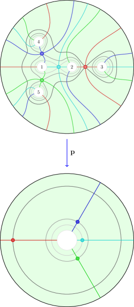
Figure 7. The metric cellular map $\mathbf{p}$ from the metric rectangular $2$-complex $\mathbf{B}_{p}$ to the compact annulus $\mathbf{A}_{p}$ with its metric rectangular cell structure. Both the domain and the range are embedded in the unit disk, even though this process distorts their intrinsic metrics.

Remark 5.3 (Multipedal pants).

The drawing of the branched annulus $\mathbb{B}_{p}$ in the disk $\mathbb{D}$ can be lifted to a surface in the solid cylinder $\mathbb{D}\times\mathbb{I}$ by adding in the height of a point under the map $\mathbb{B}_{p}\to\mathbb{A}\to\mathbb{I}$ as a third coordinate. The root circles lie in the disk at the bottom of the cylinder, the circle at infinity is boundary of the disk at the top, and the level sets are the horizontal cross-sections. For quadratic polynomials, this surface will be the “pair of pants” familiar to topologists and in general, a polynomial of degree $d$ will produce a pair of multipedal pants designed for a being with $d$ legs. An example of a $3$-legged pair of pants for a cubic polynomial is shown in Figure 8.

6. Level Sets and Direction Sets

In the remainder of the article we turn our attention to the large amount of information encoded in the metric rectangular complex $\mathbf{B}_{p}$. Latitudes and longitudes provide a pair of transverse measured foliations for $\mathbb{A}$, and their preimages under $p_{A}$ provide a pair of (singular) transverse measured foliations for $\mathbb{B}_{p}$ with singularities at the critical points of $p$. The leaves of each pullback foliation can be written as metric graphs via the cell structure for $\mathbf{B}_{p}$ and these provide valuable combinatorial data associated to the polynomial $p$. This section explores the geometry and topology of these preimages.

Definition 6.1 (Level sets and direction sets).

By composing the polynomial $p_{A}\colon\mathbb{B}_{p}\to\mathbb{A}$ with the projections $\mathbf{hgt}\colon\mathbb{A}\to\mathbb{I}$ and $\mathbf{arg}\colon\mathbb{A}\to\mathbb{S}$, we obtain maps $\mathbb{B}_{p}\to\mathbb{I}$ and $\mathbb{B}_{p}\to\mathbb{S}$. For each $t\in\mathbb{I}$ or $u\in\mathbb{S}$, define the level set of height $t$ by $\textsc{Lvl}_{t}=p_{A}^{-1}(\textsc{Lat}_{t})=\left(\mathbf{hgt}\circ p_{A}\right)^{-1}(t)$ and the direction set of argument $u$ by $\textsc{Dir}_{u}=p_{A}^{-1}(\textsc{Long}_{u})=\left(\mathbf{arg}\circ p_{A}\right)^{-1}(u)$. Since $p_{A}$ is a proper map, each of these preimages is a compact subset of $\mathbb{B}_{p}$, and note that the restricted maps $\mathbf{hgt}\circ p_{A}\colon\textsc{Lvl}_{t}\to\mathbb{S}$ and $\mathbf{arg}\circ p_{A}\colon\textsc{Dir}_{u}\to\mathbb{I}$ are discretely branched covers. We say that $\textsc{Lvl}_{t}$ (or $\textsc{Dir}_{u}$) is critical when its image is a critical latitude (or longitude), and regular otherwise. Each latitude circle and longitude line can be made into a metric graph by intersecting it with the cell structure for $\mathbf{A}_{p}$, and the results are isomorphic to $\mathbf{S}_{p}$ and $\mathbf{I}_{p}$ respectively. In the same way, each level set $\textsc{Lvl}_{t}$ and direction set $\textsc{Dir}_{u}$ inherits a cell structure from $\mathbf{B}_{p}$, turning each of them into a metric graph and making the restricted maps $p_{A}\colon\textsc{Lvl}_{t}\to\textsc{Lat}_{t}$ and $p_{A}\colon\textsc{Dir}_{u}\to\textsc{Long}_{u}$ into metric cellular maps. Note, however, that the cell structures for $\textsc{Lvl}_{t}$ and $\textsc{Dir}_{u}$ are subcomplexes of $\mathbf{B}_{p}$ if and only if they are critical.

While level sets are topologically equivalent to the usual definition for polynomial lemniscates, the metric is different.

Remark 6.2 (Lemniscates).

For a polynomial $p$, the subset $\{z\in C\mid|p(z)|=r\}$ in $\mathbb{C}$ is known as a polynomial lemniscate and its image under the inclusion map $i_{B}$ is the level set described above. While these two objects are homeomorphic, it is important to remember that the bounded metric on $\mathbb{B}_{p}$ differs from the standard metric on $\mathbb{C}$. For example, Erdős, Herzog, and Piranian asked whether the lemniscate $\{z\in\mathbb{C}\mid|p(z)|=1\}$ has maximum length when $p$ the polynomial $p(z)=z^{d}-1$, and this problem has remained open for over sixty years [EHP58]. On the other hand, every level set in $\mathbb{B}_{p}$ has total length $2\pi d$.

It is easy to provide a precise geometric description of the regular level sets and regular direction sets, but the critical versions require a bit more exposition. We begin with an elementary example.

Example 6.3 (One critical value).

Let $p(z)=a(z-b)^{d}+c$ with $a,c\in\mathbb{C}_{\mathbf{0}}$ and $b\in\mathbb{C}$. As described in Example 3.5, $b$ is the unique critical point for $p$, $c$ is the corresponding unique critical value, and $p$ has distinct roots since $c$ is nonzero. Since there is only one critical point, $\mathbf{S}_{p}$ has $1$ vertex and $1$ edge, while $\mathbf{I}_{p}$ has $3$ vertices and $2$ edges. Let $t$ and $u$ denote the height and argument of $i_{A}(c)$ in $\mathbb{A}$, respectively. Figure 8 shows the multipedal pants version of $\mathbf{B}_{p}$ when $d=3$, along with its unique critical level set $\textsc{Lvl}_{t}$ and unique critical direction set $\textsc{Dir}_{u}$. Each level set has total length $2\pi d$ and there are two regular isometry types: $\textsc{Lvl}_{s}$ is the disjoint union of $d$ copies of $\mathbf{S}_{p}$ when $s<t$ and $\textsc{Lvl}_{s}$ is isometric to $\mathbf{S}_{p}(d)$ when $s>t$. The unique critical level set for $p$ occurs at height $t$ and is isometric to the $d$-fold wedge sum of $d$ copies of $\mathbf{S}_{p}$. Meanwhile, each regular direction set is isometric to the disjoint union of $d$ copies of $\mathbf{I}_{p}$ and the unique critical direction set may be written as the wedge sum of $d$ copies of $\mathbf{I}_{p}$. This critical direction set occurs at argument $u$ and has the structure of a metric tree with $2d$ leaves, each of which is connected via an edge to a single non-leaf vertex. Half of these edges have length $t$ while the rest have length $2-t$, and the two types alternate in the local cyclic ordering around the non-leaf vertex.

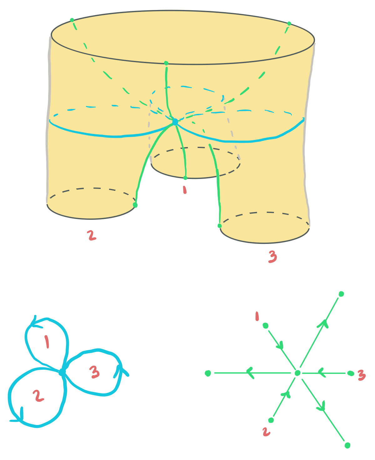
Figure 8. The branched annulus for a cubic polynomial of the form described in Example 6.3, along with its unique critical level set and direction set.

By Lemma 4.13, Example 6.3 also describes the generic local picture for what level sets and direction sets look like near the image of a critical point in $\mathbf{B}_{p}$. We begin with the regular case.

Lemma 6.4 (Product preimages).

Let $T\subset\mathbb{I}$ and $U\subset\mathbb{S}$ be connected subsets such that the product region $T\times U\subset\mathbb{A}$ is disjoint from $i_{A}(\mathbf{cvl})$. If $U$ is a proper subset of $\mathbb{S}$, then the preimage $p_{A}^{-1}(T\times U)$ has $d$ connected components, each of which is isometric to the rectangle $T\times U$. If $U=\mathbb{S}$, then there are positive integers $k_{1},\ldots,k_{m}$ with $k_{1}+\cdots+k_{m}=d$ such that the preimage $p_{A}^{-1}(T\times U)$ is isometric to the disjoint union of annuli $(T\times\mathbb{S}(k_{1}))\sqcup\cdots\sqcup(T\times\mathbb{S}(k_{m}))$.

Proof.

First, note that the restricted map $p_{A}\colon p_{A}^{-1}(T\times U)\to T\times U$ is a $d$-fold covering map and a local isometry. If $U$ is a proper subset of $\mathbb{S}$, then $T\times U$ is simply-connected and thus the preimage under $p_{A}$ must consist of $d$ isometric copies of $T\times U$. If $U=\mathbb{S}$, then $T\times U$ is an annulus of circumference $2\pi$, so each connected component of the preimage is an annulus with circumference equal to an integer multiple of $2\pi$. ∎

Note that the rectangles and annuli described might be degenerate if $T$ or $U$ (or both) is only a single point. Next, we add in the cell structure. Recall that $\mathbf{A}_{p}=\mathbf{I}_{p}\times\mathbf{S}_{p}$. By composing $\mathbf{p}\colon\mathbf{B}_{p}\to\mathbf{A}_{p}$ with the projection onto either factor, there are natural cellular maps from the branched annulus to the interval and to the circle. The preimages of open edges under these compositions can easily be characterized, providing a concrete description of both regular level sets and regular direction sets. The following two results are immediate consequences of Lemma 6.4.

Lemma 6.5 (Regular level sets).

If $T$ is an open edge in $\mathbf{I}_{p}$, then its preimage in $\mathbf{B}_{p}$ is a union of disjoint annuli, and each annulus is a direct metric product of the open edge $T$ with a finite-sheeted cover of $\mathbf{S}_{p}$. More precisely, there exist positive integers $k_{1},\ldots,k_{m}$ with $k_{1}+\cdots+k_{m}=d$ such that the preimage of $T$ is a disjoint union of annuli $(T\times\mathbf{S}_{p}(k_{1}))\sqcup\cdots\sqcup(T\times\mathbf{S}_{p}(k_{m}))$. As a consequence, for each point $t\in T$, the regular level set $\textsc{Lvl}_{t}$ looks like $\mathbf{S}_{p}(k_{1})\sqcup\cdots\sqcup\mathbf{S}_{p}(k_{m})$ and its metric cell structure is independent of the choice of $t\in T$.

Lemma 6.6 (Regular direction sets).

If $U$ is an open edge in $\mathbf{S}_{p}$, then its preimage in $\mathbf{B}_{p}$ is a union of $d$ disjoint rectangles, and each rectangle is a metric product of $\mathbf{I}_{p}$ and the open edge $U$. As a consequence, for each point $u\in U$, the regular direction set $\textsc{Dir}_{u}$ looks like $\mathbf{I}_{p}\sqcup\cdots\sqcup\mathbf{I}_{p}$ and its metric cell structure is independent of the choice of $u\in U$.

Removing a regular direction set leaves a branched cover of a rectangle.

Lemma 6.7 (Removing a regular direction set).

Let $T$ be an open edge in $\mathbf{S}_{p}$. When the preimage of $T\times\mathbf{I}_{p}$ under $\mathbf{p}$ is removed from the branched annulus $\mathbf{B}_{p}$, the result is a contractible, connected branched cover of the rectangle $\mathbf{A}_{p}\setminus(T\times\mathbf{I}_{p})$.

Proof.

By Lemma 6.5 the inverse image of the strip $T\times\mathbf{I}_{p}$ under $\mathbf{p}$ consists of $d$ disjoint copies of the strip, with each copy connecting a $T$-edge in a root circle to one of the $d$ $T$-edges in the circle at infinity. Moreover, distinct strips start at distinct root circles, since each root circle has a unique edge sent to the copy of $T$ in $\textsc{Lat}_{-1}$. The fundamental group of the branched annulus $\mathbf{B}_{p}$ is a rank $d$ free group generated by loops running around the root circles, but each strip that is removed cuts the surface and reduces the rank of this free group. The final surface is connected and contractible with a single boundary cycle, and it is a branched cover by Proposition 4.1. Notice that when $\mathbf{S}_{p}$ has only one edge, the ‘rectangle’ $\mathbf{A}_{p}\setminus(T\times\mathbf{I}_{p})$ is degenerate, being only a single copy of $\mathbf{I}_{p}$. The result still holds, but the ‘surface’ degenerates into a planar tree. ∎

Critical level sets and critical direction sets are more complicated due to the branch points. A connected component of a critical level set is a special type of metric graph that we call a metric cactus. A metric cactus may be of the form $\mathbf{S}_{p}(k)$, as in the regular case, but it can also contain branch points, as in Figure 8.

Definition 6.8 (Metric cacti).

A cactus diagram is a contractible $2$-dimensional cell complex embedded in the plane where each edge lies in the boundary of a unique $2$-cell. As a consequence of these restrictions, the boundary of an open $2$-cell is a (simple) cycle, disjoint open $2$-cells have closures that intersect in at most one point, and the closed $2$-cells are assembled in a “tree-like” fashion. In graph theory a cactus is a graph where every edge belongs to a unique cycle, and the $1$-skeleton of a cactus diagram is an example. Note that loops and multiple edges are permitted. Actually, the $1$-skeleton of a cactus diagram can be viewed as a directed graph by giving a counter-clockwise orientation to the boundary cycle of each $2$-cell. Let $\mathbf{S}$ be a circle of length $2\pi$ with a fixed cell structure and consistently oriented edges. If $\Gamma$ is a branched cover of $\mathbf{S}$ and it is also the oriented $1$-skeleton of a cactus diagram, then we call $\Gamma$ a metric cactus. Note that every simple cycle in $\Gamma$ is a copy of $\mathbf{S}(k)$ for some positive integer $k$.

Cactus diagrams and cactus graphs appear in [Nek14], but it is worth noting that they are put to a different use. Cactus cycles in [Nek14] correspond to post-critical points of $p$, whereas ours are closely connected to roots.

Lemma 6.9 (Critical level sets).

Inside $\mathbf{B}_{p}$, every component of every level set is a metric cactus. Moreover, each critical point of multiplicity $k$ labels a cactus vertex of valence $2(k+1)$ and it belongs to exactly $k+1$ distinct cycles.

Proof.

The topological part of the proof is Morse-theoretic. For each $r\geq 0$, let $C(r)=\{z\mid|p(z)|\leq r\}\subset\mathbb{C}$. When $r$ is positive, we upgrade $C(r)$ from a topological subset of the plane to a planar cell complex by giving its boundary the cell structure of the corresponding critical level set in $\mathbf{B}_{p}$. Note that every connected component of $C(r)$ is contractible since a bounded complementary component would lead to a contradiction of the Maximum Modulus Principle. In particular, as $r$ continues to increase, the bounded region eventually must disappear and the final points to disappear will be isolated since the critical points of $p$ are discrete. Such points would have a locally maximal modulus, thus provoking a contradiction. When $r=0$, $C(r)$ is the discrete set of roots and as $r$ increases, it immediately becomes a set of $d$ disjoint closed topological disks. Note that each connected component is a cactus diagram with only one $2$-cell. As $r$ increases further, some of the growing closed disks intersect precisely when $r$ has the magnitude of a critical point of $p$. When this happens the local picture is governed by Lemma 4.13. This establishes the valence requirements and the closed disks only overlap at isolated points because the critical values of $p$ are discrete. Thus, $C(r)$ remains a cactus diagram during this transition. As a branched cover of $\mathbf{S}_{p}$ and the $1$-skeleton of a cactus diagram, the critical level set corresponding to $\partial C(r)$ is a metric cactus. As $r$ increases further, annuli are attached to the boundary cycles of the connected components, and the space $C(r)$ returns to being a disjoint union of closed topological disks, but now with strictly fewer connected components. Proceeding in this way shows that every level set is a metric cactus. ∎

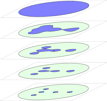
Figure 9. The critical horizontal slices of the branched annulus $\mathbf{B}_{p}$ as embedded in $\mathbb{D}\times\mathbb{I}$, together with its two extreme level sets at the top and bottom of the solid cylinder.

Remark 6.10 (Multipedal pants and cactus diagrams).

An alternative way to visualize the union of cactus diagrams that level sets bound is to use the embedding of $\mathbf{B}_{p}$ as a multipedal pair of pants inside $\mathbb{D}\times\mathbb{I}$. The pair of pants have an “inside” and an “outside”. If you add disks to the portions of horizontal slices that are on the “inside”, then the result is a union of cactus diagram. The critical level sets corresponding and the corresponding cactus diagrams for our running example are shown in Figure 9, together with the two extreme level sets at top and bottom the solid cylinder.

A connected component of a critical direction set is a special type of metric tree that we call a metric banyan. A metric banyan may be of the form $\mathbf{I}_{p}$, as in the regular case, but it can also contain branch points, as in Figure 8.

Definition 6.11 (Banyan trees).

Let $\mathbf{I}$ be a compact metric interval with a fixed cell structure and with oriented edges consistently pointing towards one of its endpoints. A metric banyan tree is a contractible branched cover of $\mathbf{I}$ together with a fixed embedding in the plane so that the incoming and outgoing edges strictly alternate in the clockwise cyclic order around one of its internal vertices. Notice that every point in a metric banyan has a well defined height given by its projection to $\mathbf{I}$. A vertex of a metric banyan tree is called a source, sink or interior vertex based on its image in $\mathbf{I}$.

Remark 6.12.

The choice of name “banyan tree” is inspired by the behavior of the real-life version, where branches grow off-shoots heading both towards and away from the ground. By adding the well-defined height as a third dimension, one may notice that the lifts of the planar trees described above mimic this behavior.

Lemma 6.13 (Critical direction sets).

Inside a branched annulus $\mathbf{B}_{p}$, every component of every direction set is a metric banyan. Moreover, each critical point of multiplicity $k$ labels an interior banyan vertex of valence $2(k+1)$.

Proof.

By Proposition 4.1, every singular component of a direction set is a branched covering of $\mathbf{I}_{p}$. The planar embedding, the local alternation of incoming and outgoing edges, and the valence requirement are all immediate, since the local picture near a branch point is governed by Lemma 4.13. It only remains to show that every component is contractible and thus a tree. This is clear for regular direction sets by Lemma 6.5, so we only need to consider the critical ones. Let $T$ be an open edge in $\mathbf{S}_{p}$ and consider the inverse image of the strip $T\times\mathbf{I}_{p}$ under $\mathbf{p}$. By Lemma 6.7, removing these $d$ strips results in a connected and contractible branched cover of a rectangle. If we repeat this process for each other open edge in $\mathbf{S}_{p}$, then these additional “cuts” increase the number of connected components, but each component remains simply connected. After all such strips have been removed, all that remains is the disjoint union of all critical direction sets. This shows that every component of every critical direction set is simply connected and contractible. ∎

We conclude this section with two brief remarks that will be explored in greater depth in future articles by the authors. The first remark highlights the underlying similarity between banyan trees and cacti.

Remark 6.14 (Banyan and cactus conversions).

Let $\Gamma$ be a level set of $\mathbf{B}_{p}$ and let $T$ be an open edge in $\mathbf{S}_{p}$. Then removing the preimages of $T\times\mathbf{I}_{p}$ (as described in Lemma 6.7) from $\mathbf{B}_{p}$ removes $d$ open edges from $\Gamma$; one can show that the resulting metric graph is a metric banyan. Conversely, if $\Gamma$ is a direction set of $\mathbf{B}_{p}$ and $T$ is an open edge in $\mathbf{S}_{p}$, then removing the preimages of $T\times\mathbf{I}_{p}$ turns $\mathbf{B}_{p}$ into a $4d$-gon that is a connected $d$-fold branched cover of the rectangle $\mathbf{A}_{p}\setminus(T\times\mathbf{I}_{p})$ (Lemma 6.7). Every fourth side of the $4d$-gon contains a source vertex of $\Gamma$, every fourth side of the $4d$-gon contains a sink vertex of $\Gamma$ and none of these $2d$ sides are adjacent. One can add a collection of $d$ isometric metric edges to $\Gamma$ connecting each source vertex to the “next” sink vertex in the counter-clockwise order. This can be done simultaneously in a plane and the result is a graph where each component is a metric cactus. This close connection between metric banyans and metric cacti is less surprising once one uses Lemma 6.7 to restrict a branched annulus to a branched rectangle. There is an obvious symmetry between the horizontal and vertical foliations of the rectangle and this produces a symmetry between metric banyans and restricted portions of metric cacti.

The second remark focuses on realizability.

Remark 6.15 (Banyan and cactus realizations).

One can prove stronger versions of Lemma 6.9 and Lemma 6.13 that include an assertion about the converse direction. Concretely, after adding mild and obvious restrictions, every metric cactus and every metric banyan arises as a component of a level set or a direction set for some complex polynomial $p$.

7. Partitions

The branched annulus of a complex polynomial contains a wealth of combinatorial (and geometric) data encoded in its level sets and direction sets. In this section we extract some of this combinatorial data and highlight an intrinsic connection between the geometry of complex polynomials and the combinatorics of noncrossing partitions. We begin with partitions.

Definition 7.1 (Partitions).

Let $A$ be a set of size $d$. A partition of $A$ is a collection of pairwise disjoint subsets (called blocks) whose union is $A$. Let $\Pi_{A}$ denote the set of all such partitions. Given partitions $\lambda,\mu\in\Pi_{A}$, $\lambda$ is a refinement of $\mu$ if each block of $\lambda$ is contained in some block of $\mu$. When this occurs we write $\lambda\leq\mu$, or $\lambda<\mu$ when $\lambda$ and $\mu$ are not equal. This defines a partial order which makes $\Pi_{A}$ into a lattice since meets and joins are well-defined. The unique minimum partition is the discrete partition where every block is a singleton, and the unique maximum partition is the trivial partition where there is only one block. A chain of partitions is a sequence $\lambda_{1}<\cdots<\lambda_{k}$.

The focus here is on $\Pi_{\mathbf{rts}}$, the partition lattice of the roots of $p$.

Definition 7.2 (Partitions from level sets).

As described in the proof of Lemma 6.9, for every $t\in\mathbb{I}^{\textrm{int}}$, the level set $\textsc{Lvl}_{t}$ of $p$ can be viewed as the boundary of a disjoint union of cactus diagrams in $\mathbb{C}$ and every root is contained in the interior of one of these diagrams. We define a partition $\lambda_{t}$ by placing two roots in the same block if and only if they are contained in the same connected component, i.e. the same cactus diagram. Note that as $t$ increases, the cactus diagrams grow and merge but they do not split, and, as a consequence $\lambda_{t}$ can only increase in the partial order on $\Pi_{\mathbf{rts}}$.

Remark 7.3 (Regular level sets as separating multicurves).

A multicurve is a disjoint union of simple closed curves on a given (connected) surface, and a multicurve is separating if its complement is disconnected. Since each latitude $\textsc{Lat}_{t}$ in the open annulus $\mathbb{A}^{\textrm{int}}$ disconnects the (closed) annulus $\mathbb{A}$, its preimage $\textsc{Lvl}_{t}$ separates $\mathbb{B}_{p}$. Moreover, when $t$ is regular, $\textsc{Lvl}_{t}$ is a separating multicurve. The partition $\lambda_{t}$ can then be viewed as having blocks where two roots belong to the same block if and only if the corresponding root circles belong to the same complementary component of $\textsc{Lvl}_{t}$.

Remark 7.4 (Partitions and $\mathbf{I}_{p}$).

For every point $t\in\mathbf{I}_{p}$ there is a partition $\lambda_{t}\in\Pi_{\mathbf{rts}}$. As is usual in Morse theory, the cactus diagrams remain homotopic so long as $t$ does not increase through a critical value. Thus every point in an open edge of $\mathbf{I}_{p}$ is assigned the same partition, and this partition agrees with the partition assigned to its lower endpoint. Moreover, the partition assigned to the first open edge (with $-1$ as an endpoint) is the discrete partition and the partition assigned to the last open edge (with $1$ as an endpoint) is the trivial partition. On the other hand, as $t$ approaches an interior vertex of $\mathbf{I}_{p}$ from below, there are distinct components that are merging together, which means that the partition assigned to this interior vertex is strictly higher inside $\Pi_{\mathbf{rts}}$ compared to the partition assigned to the open edge directly below it. As a consequence, the partitions assigned to the open edges of $\mathbf{I}_{p}$ are distinct representatives of every partition assigned to a level set, and they naturally form a chain in $\Pi_{\mathbf{rts}}$.

We give two examples.

Example 7.5.

Let $p(z)=a(z-b)^{d}+c$ be as in Example 6.3, and let $t$ be the height of $i_{A}(c)$, its unique critical value. There are only two open edges in $\mathbf{I}_{p}$. The partition assigned is discrete on the half-open interval $[-1,t)$ and trivial on the closed interval $[t,1]$. Thus the chain of partitions is simply: $\textrm{Discrete}<\textrm{Trivial}$.

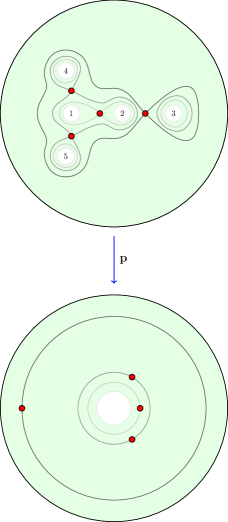
Figure 10. The union of all critical level sets in the branched annulus $\mathbf{B}_{p}$. The regular level sets between them determine a chain in $\Pi_{\mathbf{rts}}$.

Example 7.6.

The critical level sets for our standard running example are shown in Figure 10. As should be clear from the figure, the associated chain in $\Pi_{\mathbf{rts}}$ is:

$$\textrm{Discrete}<\{\{a_{1},a_{2}\},\{a_{3}\},\{a_{4}\},\{a_{5}\}\}<\{\{a_{1},a_{2},a_{4},a_{5}\},\{a_{3}\}\}<\textrm{Trivial}.$$

Remark 7.7 (Big lemniscate configurations).

The chain of partitions produced by the regular level sets of $p$ is a natural combinatorial object, although we are unaware of any explicit references to it in the literature. It is worth noting that this chain is related to what Catanese and Paluszny refer to as a “big lemniscate configuration” in [CP91], although they restrict their consideration to the lemniscate-generic case, where the combinatorics are simpler. A lemniscate-generic polynomial of degree $d$ has $d-1$ distinct critical values, all of multiplicity one, and these critical values all have distinct moduli. The cell structure of $\mathbf{I}_{p}$, in this case, has $d$ open edges and the associated chain in $\Pi_{\mathbf{rts}}$ is a maximal chain.

With a little more work, the chain of partitions determined by the regular level sets of $\mathbf{B}_{p}$ can be converted into a chain of noncrossing partitions.

Definition 7.8 (Noncrossing partitions).

Let $A$ be the vertices of a convex $d$-gon in the plane. A partition $\lambda\in\Pi_{A}$ is noncrossing if for every pair of distinct blocks in $\lambda$, the convex hull of the vertices in one block is disjoint from the convex hull of the vertices in the other. The collection of noncrossing partitions inside $\Pi_{A}$ form an induced subposet. We write $\textsc{NC}_{A}$ for this subposet, where $A$ is now viewed as a set with a fixed cyclic ordering. If $A$ is any finite set of size $d$ and we fix a cyclic ordering of its elements, then we can use this cyclic ordering to label the vertices of a $d$-gon and then create an induced noncrossing subposet of $\Pi_{A}$.

Lemma 7.9 (Open edges and cyclic orderings).

If $u\in\mathbf{S}_{p}$ is not a vertex, then $\textsc{Dir}_{u}$ is a regular direction set, and $\textsc{Dir}_{u}$ determines a natural cyclic ordering of the roots of $p$. In addition, points in the same open edge of $\mathbf{S}_{p}$ determine the same cyclic ordering of $\mathbf{rts}$.

Proof.

Let $U$ be the open edge of $\mathbf{S}_{p}$ that contains $u$. The preimage of the strip $U\times\mathbf{I}_{p}\subset\mathbb{A}$ consists of $d$ disjoint rectangular strips in $\mathbf{B}_{p}$. Each strip connects a unique copy of $U$ on a root circle to one of $d$ copies of $U$ on the circle at infinity. The bijection from roots to root circle thus extends to copies of $U$ in the circle at infinity. And note that the same bijection is produced if we use only use the regular direction set $\textsc{Dir}_{u}$ for any $u\in U$. Reading counter-clockwise around the circle at infinity thus produces a cyclic ordering of the set $\mathbf{rts}$ of roots. ∎

We illustrate the cyclic ordering of the roots using our running example.

Example 7.10 (Cyclic orderings).

In our running example, there are four open edges in $\mathbf{S}_{p}$ and thus four cyclic orderings of the roots. For readability, we label the five roots $a$, $b$, $c$, $d$ and $e$ instead of $a_{1}$, $a_{2}$, $a_{3}$, $a_{4}$ and $a_{5}$, respectively. Starting at the positive $x$-axis and proceeding counter-clockwise around the boundary, these four cyclic orderings are: $(c,a,d,e,b)$, $(c,d,a,e,b)$, $(b,d,a,e,c)$, and $(b,d,e,a,c)$. See Figure 11. In the electronic version of this article, where the colors are visible, the first cyclic ordering is determined by the regular direction sets sandwiched between the critical direction sets that are aqua and dark blue, respectively. The second is between dark blue and red, the third is between red and green and the fourth is between green and aqua.

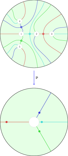
Figure 11. The union of all critical direction sets in the branched annulus $\mathbf{B}_{p}$. The regular level sets between them determine four different cyclic orderings of the set $\mathbf{rts}$.

By combining the combinatorial information coming from a regular direction set with that coming from a regular level set we can see that all of these root partitions are noncrossing.

Proposition 7.11 (Level sets and noncrossing partitions).

The partition of the roots determined by a regular level set is noncrossing with respect to the cyclic ordering of the roots determined by a regular direction set.

Proof.

Fix $u\in\mathbf{S}_{p}$ and $t\in\mathbf{I}_{p}$ so that neither one is a vertex. By Lemma 7.9, $u$ determines a corresponding cyclic ordering of the set $\mathbf{rts}$ and by Definition 7.8 this determines a subposet $\textsc{NC}_{\mathbf{rts}}$ inside $\Pi_{\mathbf{rts}}$. Let $C$ be the union of the latitude circle $\textsc{Long}_{t}$ and the longitude line $\textsc{Lat}_{u}$, and let $B=p_{A}^{-1}(C)$. A connected component of $B$ contains both the $1$-skeleton of a single cactus diagram, and the lines that connect some of the root circles to preimages of $u$ in the circle at infinity. These connected components show how to view a block of the partition $\lambda_{t}$ as a collection of preimages of $u$ in the circle at infinity. Since all of the components of $B$ are drawn in the disk without crossing, the convex hulls of the collections of points in the circle at infinity also do not cross. In particular, $\lambda_{t}$ is in the subposet $\textsc{NC}_{\mathbf{rts}}$. ∎

The following corollary is now immediate.

Corollary 7.12 (Chains of noncrossing partitions).

The chain of partitions determined by the regular level sets is noncrossing with respect to the cyclic ordering of the roots determined by any regular direction set.

Remark 7.13.

It is worth noting that connections between complex polynomials and noncrossing partitions have appeared elsewhere in the literature (e.g. [MSS07] and [Sav09]), although in slightly different manners. We are unaware of any previous results in the literature that are similar to Proposition 7.11 and Corollary 7.12.

8. Factorizations

We now shift our attention from the chain of noncrossing partitions determined by the collection of regular level sets to the factorization of a $d$-cycle determined by the collection of regular direction sets. As a first step we note that the cyclic orderings described in Lemma 7.9 can be converted to linear orderings by focusing on a particular edge in the circle at infinity.

Definition 8.1 (Linear orderings).

Let $U^{\prime}$ be an open edge in the circle at infinity in $\mathbf{B}_{p}$ and let $U$ be the open edge $\mathbf{S}_{p}$ to which it projects. First label the preimages of $U$ in the circle at infinity using the bijection from Lemma 7.9. Starting at $U^{\prime}$ and proceeding in a counter-clockwise fashion, we record the linear order in which the root labels occur. We use square brackets, rather than parentheses, to indicate that this is a linear ordering rather than a cyclic ordering.

The various linear orderings of the roots determined by the edges in the circle at infinity, can be used to create a sequence of permutations whose product is an $d$-cycle. We begin by showing how that works in our running example.

Example 8.2.

The circle at infinity in our running example has $20$ open edges. Using the same conventions as in Example 7.10, we have, for the edge in the domain in the first quadrant with one endpoint on the positive real axis, the linear order is $[c,a,d,e,b]$. Then next several linear orders, proceeding in a counter-clockwise fashion, are $[c,d,a,e,b]$, $[b,d,a,e,c]$, $[b,d,e,a,c]$ and $[a,d,e,b,c]$. There are $15$ more linear orders. Of course, the fifth linear order is just a cyclic permutation of the first since they correspond to the same set of cyclically ordered edges. Adjacent linear orders in this list give a description of a permutation of the set $\{1,2,3,4,5\}$ of positions in two line notation. The permutation from the first to the second linear order is $(2,3)$ since the $a$ and $d$ entries in positions $2$ and $3$ are swapped. The next permutation is $(1,5)$, swapping $c$ and $b$, then $(3,4)$ swapping $a$ and $e$, and finally $(1,4)$ swapping $a$ and $b$. Note that the product (with the appropriate choice of conventions for multiplying permutations) is $(1,4)(3,4)(1,5)(2,3)=(1,2,3,4,5)$ as expected.

Remark 8.3 (Banyans and permutations).

Given the fact that critical direction sets separate adjacent linear and cyclic orderings, these permutations can actually be read off of the corresponding banyan trees, specifically from the banyan trees that include branch points. For example, the dark blue critical direction set has only one branched component, the one with source vertices on the $a_{1}=a$ and $a_{4}=d$ root circles. As a consequence, the difference between the first linear order $[c,a,d,e,b]$ and the second $[c,d,a,e,b]$ involves a swapping of the roots $a$ and $d$.

In order to describe the permutations these trees produce, we first introduce a new noncrossing object, known in the literature as a primitive $d$-major.

Definition 8.4 (Real noncrossing partitions).

Let $d$ be a positive integer, let $\mathbb{S}(d)\subset\mathbb{C}$ be the circle of radius $d$ (and circumference $2\pi d$), and let $\mathbb{S}(d)\to\mathbb{S}$ be the natural covering map sending $z\mapsto(z/d)^{d}$. For each point $u\in\mathbb{S}$, its $d$ preimages are equally spaced around $\mathbb{S}(d)$ and they form the vertex set of regular $d$-gon. Thus we can define a noncrossing partition on the preimages of $u$. A real noncrossing partition $\lambda$ a choice of a noncrossing partition for each point $u\in\mathbb{S}$ subject to a compatibility condition, which requires that the convex hull of every block of every selected noncrossing partition can be simultaneously drawn inside the disk that $\mathbb{S}(d)$ bounds, while remaining pairwise disjoint. One consequence of this compatibility condition is that all but finitely many of the selected noncrossing partitions must be the discrete partition. Note that the set of all real noncrossing partitions comes with a natural partial order. One real noncrossing partition is less than or equal to another if for each $u\in\mathbb{S}$ the noncrossing partition selected by the first is less than or equal to the noncrossing partition selected by the second in the noncrossing partition lattice based on the preimages of $u$.

Remark 8.5.

Real noncrossing partitions have already appeared in the literature with a different definition and under a different name. In [TBG⁺19] they are called primitive $d$-majors. If each of the non-trivial convex hulls in the noncrossing partitions of a real noncrossing partition are shrunk to a point in a planar fashion, the result is a cactus diagram with a metric cactus as its boundary. In fact, real noncrossing partition are in natural bijection with metric cacti that are branched $d$-fold covers of $\mathbb{S}$.

Definition 8.6 (Banyans and real noncrossing partitions).

For each $u\in\mathbb{S}$, consider the $d$ points in $\textsc{Dir}_{u}$ which lie on the circle at infinity. Define a partition of these points so that two points belong to the same block if and only if they lie on the same connected component of $\textsc{Dir}_{u}$. For regular direction sets, this is the trivial partition. The proof that these partitions are noncrossing is essentially the same as in the proof of Proposition 7.11. Since all of the components of $\textsc{Dir}_{u}$ are drawn in the disk without crossing, the convex hulls of the corresponding collections of points in the circle at infinity also do not cross. This also shows that the noncrossing partitions associated to different points $u$ are compatible, so that the full banyan foliation of $\mathbb{B}_{p}$ determines a real noncrossing partition associated to the polynomial $p$.

The factorization of the $d$-cycle illustrated in Example 8.2 is closely related to the real noncrossing partition of the banyan foliation. The following result precisely describes the relationship, even though its proof is merely sketched.

Proposition 8.7 (Real noncrossing partitions and noncrossing hypertrees).

Let $\lambda$ be the real noncrossing partition associated to the foliation of $\mathbb{B}_{p}$ by banyan trees. If $u\in\mathbf{S}_{p}$ is a point that is not a vertex, then $\lambda$ corresponds to a noncrossing hypertree and a factorization of a $d$-cycle.

Proof sketch.

Since $u$ in not a vertex in $\mathbf{S}_{p}$, the noncrossing partition associated to $u$ is discrete, and the preimages of $u$ can be removed from the circle at infinity without removing a vertex of a non-trivial block of $\lambda$. The remaining portions of the circle at infinity consist of $d$ open metric arcs of length $2\pi$. Cyclically label these arcs $1,2,\ldots,d$. We use these numbers to label the vertices of each non-trivial block in $\lambda$. If we collapse the open arcs to points while maintaining planarity, the non-trivial blocks of $\lambda$ will overlap on vertices and become a noncrossing hypertree. The non-trivial blocks of $\lambda$ can also be turned into cyclic permutations, and the product of these permutations in the appropriate order produces the $d$-cycle. See [McC17] for details. ∎

This completes the proof of Theorem C. We conclude the section with two remarks on interpreting and using these results.

Remark 8.8 (Different noncrossing partitions).

The factorization of a $d$-cycle produced by a noncrossing hypertree is a minimum reflection length factorization of a $d$-cycle. There is a well-known connection between such factorizations and chains in the noncrossing partition lattice $\textsc{NC}_{[d]}$ and this is another realization of this connection. We should caution, however, that the chain in the noncrossing partition lattice determined the regular level sets (and an edge in $\mathbf{S}_{p}$) is not related to the noncrossing partition lattice corresponding to a factorization of a $d$-cycle determined by the linear orders coming from a consecutive sequence of edges in the circle at infinity. This is easiest to see in the completely generic case where every critical value has multiplicity one and all of their moduli and all of their arguments are distinct. The chain in the partition lattice is determined by the linear ordering of the critical values by latitude, whereas the factorization of the $d$-cycle is determined, in part, by the cyclic ordering of the critical values by longitude. In a future article, where we consider continuously varying a polynomial, it will be made clear how one of these two can change while the other remains fixed.

Remark 8.9 (Dual braid complex).

In a future article, we will give the space of all real noncrossing partitions a natural topology and cell structure, and identify this space with a version of the dual braid complex - see [Bra01], [BM10], and [DMW20] for details on this complex. We will use this identification to prove that the complexified hyperplane complement of the braid arrangement deformation retracts to the pure version of the dual braid complex. The tools developed in this article, and in our earlier work, will be crucial to our proofs.

9. Monodromy

In this final section we comment on the ways in which the monodromy action can be read off from the structure of the branched annulus of $p$. Our discussion here will be somewhat brief, since similar material was detailed by Elias Wegert in a recent article in the Notices of the AMS [Weg20].

Definition 9.1 (Monodromy).

Given a covering map $f\colon Y\to X$ and a point $x\in X$, each oriented loop based at $x$ lifts to a collection of directed paths in $Y$, and each path connects one preimage of $x$ to another preimage of $x$, possibly the same one. Thus, each loop can used to determine a permutation of the points in the set $A=f^{-1}(x)$, these permutations are well-defined up to homotopies of paths, and they compose as expected. The result is a group homomorphism from $\pi_{1}(X,x)$ to $\textsc{Sym}_{A}$. This is the monodromy action of the fundamental group of $X$ on the preimages of $x$.

Remark 9.2 (Polynomial monodromy).

In the case of a polynomial $p\colon\mathbb{C}\to\mathbb{C}$ with $d$ distinct roots, we know that $p$ is a discretely branched covering map; the restriction of $p$ obtained by removing the critical values and their preimages is a covering map, and thus it has a corresponding monodromy action. Since $p$ has distinct roots, $0$ is not a critical value, and we may choose $0$ to be the basepoint in the image and the fundamental group $\pi_{1}(\mathbb{C}_{\mathbf{cvl}},0)$, is a free group whose rank is equal to the number of critical values.

The monodromy action is encoded in the cell structure of the branched annulus.

Remark 9.3 (Monodromy and branched annuli).

The lower boundary circle of the annulus $\mathbb{A}$ corresponds to $0$ in a precise sense, so we can replace directed loops based at $0$ with directed paths that start and end on $\textsc{Lat}_{-1}$. The lifts of such paths will start and end at root circles and thus define a permutation of the roots. Since every branch point of the cellular map $\mathbf{p}\colon\mathbf{B}_{p}\to\mathbf{A}_{p}$ is a vertex, it is sufficient to choose paths which are suitably generic and transverse to the cell structure. These generic paths avoid the $0$-skeleton of $\mathbf{A}_{p}$ and lift to paths that avoid the $0$-skeleton of $\mathbf{B}_{p}$. Every element of the free group $\pi_{1}(\mathbb{C}_{\mathbf{cvl}},0)$ has such a transverse representative and the combinatorial nature of the cell structures involved make the permutation determined by the lifts easy to determine.

We illustrate this idea with two simple examples.

Example 9.4.

In our running example, consider the path in $\mathbb{C}$ that starts at the origin, increases along the positive real axis, circles the unique critical value on this ray in a counter-clockwise fashion and then returns to the origin along the real axis. In $\mathbf{A}_{p}$ there is an equivalent path that proceeds up the corresponding longitude, circles around the critical value and then returns to $\textsc{Lat}_{-1}$ along this longitude. This path in $\mathbf{A}_{p}$ lifts to a set of $5$ paths in $\mathbf{B}_{p}$. The path that start on the $a_{3}$ root circle, returns to the $a_{3}$ root circle, as do the paths that start on $a_{4}$ root circle and the $a_{5}$ root circle. The path that starts on the $a_{1}$ root circle ends on the $a_{2}$ root circle and vice versa. This is because of the branch point between them. Thus, the corresponding permutation is $(a_{1},a_{2})$.

And finally, we conclude with comment on a connection between the monodromy and the structure of the banyan trees in $\mathbf{B}_{p}$.

Example 9.5.

Let $u$ be a vertex in $\mathbf{S}$ and consider the path in $\mathbf{A}_{p}$ that starts just to the right of the copy of $u$ in $\textsc{Lat}_{-1}$, travels straight up until its height exceeds that of all the critical values on $\textsc{Long}_{u}$, crosses over to the righthand side of $\textsc{Long}_{u}$ and then returns straight down to the lefthand side of $u$ in $\textsc{Lat}_{-1}$. The permutation determined by this path is the same as the noncrossing permutation that corresponds to the noncrossing partition associated with the critical direction set $\textsc{Dir}_{u}$ as part of the real noncrossing partition associated to the polynomial $p$. In particular, this permutation is completely determined by the structure of the non-trivial banyan trees in the critical direction set $\textsc{Dir}_{u}$. Any other directed path in $\mathbf{A}_{p}$ that stays close to the critical longitude $\textsc{Long}_{u}$ also determines a permutation that can be read off of the structure of the metric banyan trees comprising the critical direction set $\textsc{Dir}_{u}$.

References

- [BCN02] A. F. Beardon, T. K. Carne, and T. W. Ng, The critical values of a polynomial, Constr. Approx. 18 (2002), no. 3, 343–354.
- [BM10] Tom Brady and Jon McCammond, Braids, posets and orthoschemes, Algebr. Geom. Topol. 10 (2010), no. 4, 2277–2314.
- [Bra01] Thomas Brady, A partial order on the symmetric group and new ’s for the braid groups, Adv. Math. 161 (2001), no. 1, 20–40.
- [CP91] Fabrizio Catanese and Marco Paluszny, Polynomial-lemniscates, trees and braids, Topology 30 (1991), no. 4, 623–640.
- [CW91] Fabrizio Catanese and Bronislaw Wajnryb, The fundamental group of generic polynomials, Topology 30 (1991), no. 4, 641–651.
- [DMW20] Michael Dougherty, Jon McCammond, and Stefan Witzel, Boundary braids, Algebr. Geom. Topol. 20 (2020), no. 7, 3505–3560.
- [EHL18] Michael Epstein, Boris Hanin, and Erik Lundberg, The lemniscate tree of a random polynomial, Preprint (2018), 18 pages.
- [EHP58] P. Erdős, F. Herzog, and G. Piranian, Metric properties of polynomials, J. Analyse Math. 6 (1958), 125–148. MR 101311
- [EMHZZ96] Mohamed El Marraki, Nicolas Hanusse, Jörg Zipperer, and Alexander Zvonkin, Cacti, braids and complex polynomials, Sém. Lothar. Combin. 37 (1996), Art. B37b, 36. MR 1462334
- [Hum03] Stephen P. Humphries, Finite Hurwitz braid group actions on sequences of Euclidean reflections, J. Algebra 269 (2003), no. 2, 556–588.
- [McC17] Jon McCammond, Noncrossing hypertrees, preprint (2017), 53 pages.
- [Mic06] J. Michel, Hurwitz action on tuples of Euclidean reflections, J. Algebra 295 (2006), no. 1, 289–292.
- [MSS07] Jeremy L. Martin, David Savitt, and Ted Singer, Harmonic algebraic curves and noncrossing partitions, Discrete Comput. Geom. 37 (2007), no. 2, 267–286.
- [Nek14] Volodymyr Nekrashevych, Combinatorial models of expanding dynamical systems, Ergodic Theory Dynam. Systems 34 (2014), no. 3, 938–985.
- [Sav09] David Savitt, Polynomials, meanders, and paths in the lattice of noncrossing partitions, Trans. Amer. Math. Soc. 361 (2009), no. 6, 3083–3107.
- [TBG+19] William P. Thurston, Hyungryul Baik, Yan Gao, John H. Hubbard, Tan Lei, Kathryn A. Lindsey, and Dylan P. Thurston, Degree--invariant laminations, preprint (2019), 62 pages.
- [Weg20] Elias Wegert, Seeing the monodromy group of a Blaschke product, Notices Amer. Math. Soc. 67 (2020), no. 7, 965–975.
- [Zvo00] Alexander Zvonkin, Towards topological classification of univariate complex polynomials, Formal power series and algebraic combinatorics (Moscow, 2000), Springer, Berlin, 2000, pp. 76–87. MR 1798203