Tight constraints on Einstein-dilation-Gauss-Bonnet gravity from GW190412 and GW190814

Abstract

Gravitational-wave (GW) data can be used to test general relativity in the highly nonlinear and strong field regime. Modified gravity theories such as Einstein-dilation-Gauss-Bonnet and dynamical Chern-Simons can be tested with the additional GW signals detected in the first half of the third observing run of Advanced LIGO/Virgo. Specifically, we analyze gravitational-wave data of GW190412 and GW190814 to place constraints on the parameters of these two theories. Our results indicate that dynamical Chern-Simons gravity remains unconstrained. For Einstein-dilation-Gauss-Bonnet gravity, we find $\sqrt{\alpha_{\rm EdGB}}\lesssim 0.40\,\rm km$ when considering GW190814 data, assuming it is a black hole binary. Such a constraint is improved by a factor of approximately $10$ in comparison to that set by the first Gravitational-Wave Transient Catalog events.

I Introduction

Gravitational-waves (GWs) data have been widely used to test general relativity (GR) in the strong gravity regime. No significant deviations from GR have been found from analyses based on events from the first Gravitational-Wave Transient Catalog (GWTC-1) (Abbott et al., 2016, 2019a, 2019b). Recently, about $39$ GW events were reported by Advanced Laser Interferometer Gravitational-Wave Observatory (LIGO) and Advanced Virgo (Abbott et al., 2020a). Among them, there are three events/candidates involving the merger of one neutron star (NS) or light mass black hole (BH) with another compact object (GW190425 (Abbott et al., 2020b; Han et al., 2020), GW190426_152155, and GW190814 (Abbott et al., 2020c)), three GW events with mass ratios greater than $3$ (GW190412 (Abbott et al., 2020d), GW190426_152155, and GW190814), and one merger producing an intermediate mass black hole (GW190521 (Abbott et al., 2020e, f)). Based on these new data, dedicated analyses have been carried out to improve the general constraints on the deviations from GR based on model independent tests (Abbott et al., 2020).

Employing the publicly available posterior probability distributions released from the LIGO-Virgo Collaboration (LVC) (Abbott et al., 2019c, 2020a, b, 2020), one can set constraints on some specific modified gravity theories with the reweighting method. A more reliable method to constrain the theory is to perform a Bayesian analysis with modified GW waveform on real GW data. However, a full analytic inspiral-merger-ringdown (IMR) waveform model is not available even in the GR case since a prediction of the gravitational radiation during the merger stage is too complicated to be performed analytically. Currently, the merger stage is tractable only through numerical methods. The extension of such numerical methods to beyond GR theories can be achieved only provided a well-behaved formulation of the equations of motion, which is presently lacking for many alternative theories in the strong-coupling limit (Witek et al., 2019; Okounkova et al., 2019; Okounkova, 2020). The inspiral stage is well described by post-Newtonian (PN) theory (Blanchet, 2014) and the ringdown stage is fully described by a superposition of damped oscillations, i.e., the quasinormal modes (Kokkotas and Schmidt, 1999; Ferrari and Gualtieri, 2008; Berti et al., 2009). For massive sources like GW190521, the signal detected by LIGO and Virgo is dominated by the merger and ringdown stages. Instead, for most of other events, the inspiral stage is dominant since the masses of them are quite smaller than GW190521. By considering perturbative modifications to GR, the parametrized post-Einsteinian (ppE) framework (Yunes and Pretorius, 2009; Yunes et al., 2016) has been developed to incorporate the effects of certain classes of modified gravity theories on GW signals (here, we focus on the inspiral stage).

Einstein-dilation-Gauss-Bonnet (EdGB) (Kanti et al., 1996; Yagi et al., 2016) and dynamical Chern-Simons (dCS) (Alexander and Yunes, 2009) are two particularly interesting classes of alternative theories to GR. Both of them have strong theoretical motivations (arising from, for instance, the low-energy limit of string theory or proposed to accommodate the matter-antimatter asymmetry of the Universe). The modifications to GR are introduced by a scalar field nonminimally coupled to squared curvature scalars, which is why these theories are known as quadratic gravity theories. The nonvanishing scalar field results in a violation of the strong equivalence principle; thus, these two theories provide interesting models to test fundamental principles of GR. By analyzing the events contained in the GWTC-1 catalog, Nair et al. (2019) reported a constraint on EdGB, $\sqrt{\alpha_{\rm EdGB}}\lesssim 5.6\,\rm km$, the first constraint on this parameter with GW data. A reliable constraint on dCS, however, is not achievable with these events, yet.

For GW events with a fixed signal-to-noise ratio (SNR), more stringent constraints on these two theories can be imposed if at least one of the components has a low mass. When only the secondary component mass of the binary is small, at current SNRs, higher multipoles can have a sizable impact on the parameter estimation roughly for $q>3$ (Khan et al., 2020). The analyses in Abbott et al. (2020d, c) also show that both the higher multipoles and precession will affect the estimation of masses and spins of the sources, which finally affect the constraints on EdGB and dCS gravity. Furthermore, there are subtleties in casting constraints on these theories by analysing neutron star-black hole (NSBH) system. In EdGB gravity, BHs have nonvanishing scalar charges, while NSs do not if the scalar field coupling is linear (Yagi et al., 2012a), and the constraint on $\sqrt{\alpha_{\rm EdGB}}$ could be more promising for a mixed binary (Carson et al., 2020). For dCS gravity, the leading order of the scalar charge effect enters at $2$ PN while the tidal effect enters at $1$ PN (Vines et al., 2011; Damour et al., 2012), and the perturbations taking into account tidal effects have not yet been computed. So we do not perform analyses on dCS theory for NSBH cases.

In this work, we first adopt the reweighting method to analyze GW data of two selected events of GWTC-2 (i.e., GW190412 and GW190814), whose mass ratios are larger than $3$ and for which the inspiral SNRs are larger than $6$ (Abbott et al., 2020). Then we use Bayesian inference method to analyze these two events. We focus on the modification due to EdGB and dCS in the inspiral phase of GW signal, within the ppE framework. The methods we adopted are described in Sec. II, and the main results are presented in Sec. III. Finally, we summarize the results obtained in this work in Sec. IV. We assume $G=c=1$ throughout the paper, unless otherwise specified.

II Methods

For both EdGB and dCS theories, the modifications on the phase of the inspiral stage can be incorporated into the ppE formalism, which describes the gravitational waveform of theories alternative to GR in a model-independent way (Yunes and Pretorius, 2009). Indeed, the effects of the scalar dipole (in EdGB) and scalar quadrupole (in dCS) radiation are captured by the ppE parameter entering at $-1$ and $2$ PN order, respectively. Although these modifications affect the amplitudes of GW signals, the results presented in Tahura et al. (2019) show that phase-only analyses can place tight constraints. For a binary compact object with component masses $m_{1}$ and $m_{2}$ in the detector frame, the ending frequency of the inspiral stage can be approximated by $f_{\rm high}=0.018/[(m_{1}+m_{2})]$ (Abbott et al., 2019b). Above this frequency the waveform model cannot be well described by the PN expansion and the ppE formalism and needs to be included in a different way (Yunes et al., 2016). Therefore, in this work, we only consider phase corrections and analyze GW data with inspiral waveform only, since the signal sourced by these events is dominated by the inspiral radiation.

The inspiral stage of the IMR waveform model can be expressed in the form of $h_{\mathrm{ins}}(f)=A_{\mathrm{ins}}(f)e^{i{\Psi}_{\mathrm{ins}}}$; then, the waveform model including the modification due to EdGB or dCS can be written as $h_{\mathrm{ins}}(f)=A_{\mathrm{ins}}(f)e^{i{\Psi}_{\mathrm{ins}}+i\beta_{\rm EdGB,dCS}(\pi\mathcal{M}f)^{b}}$, where $b=-7/3$ ($b=-1/3$) for EdGB (dCS) gravity. The coupling constants in these two theories are $\alpha_{\rm EdGB}$ and $\alpha_{\rm dCS}$, respectively. For EdGB gravity (Yagi et al., 2012a), $\beta_{\mathrm{EdGB}}$ can be expressed as

$$\beta_{\mathrm{EdGB}}=-\frac{5}{7168}\frac{\left(m_{1}^{2}s_{2}^{\mathrm{EdGB}}-m_{2}^{2}s_{1}^{\mathrm{EdGB}}\right)^{2}}{\eta^{18/5}M^{4}}\frac{16\pi\alpha_{\mathrm{EdGB}}^{2}}{M^{4}}.$$ (1)

Here, $\eta=m_{1}m_{2}/M^{2}$ is the symmetric mass ratio, $M=m_{1}+m_{2}$ is the total mass, $\mathcal{M}=(m_{1}m_{2})^{3/5}/(m_{1}+m_{2})^{1/5}$ is the chirp mass, and $s_{i}^{\mathrm{EdGB}}=2\left(\sqrt{1-\chi_{i}^{2}}-1+\chi_{i}^{2}\right)/\chi_{i}^{2}$ are the dimensionless BH charges in EdGB gravity (Berti et al., 2018; Prabhu and Stein, 2018), where $\chi_{i}=\vec{S}_{i}\cdot\hat{L}/m_{i}^{2}$ are the dimensionless spins of BHs with spin angular momentum $\vec{S}_{i}$ in the direction of the orbital angular momentum $\hat{L}$.

For dCS gravity, the phase modification takes the form (Yagi et al., 2012b)

$$\beta_{\mathrm{dCS}}= \frac{16\pi\alpha_{\mathrm{dCS}}^{2}}{M^{4}\eta^{14/5}}\biggl{(}-\frac{5}{8192}\frac{\left(m_{1}s_{2}^{\mathrm{dCS}}-m_{2}s_{1}^{\mathrm{dCS}}\right)^{2}}{M^{2}}$$ (2)

$$+\left.\frac{15075}{114688}\left(\frac{m_{1}^{2}\chi_{2}^{2}+m_{2}^{2}\chi_{1}^{2}}{M^{2}}-\frac{350}{201}\eta\chi_{1}\chi_{2}\right)\right),$$

where $s_{i}^{\mathrm{dCS}}=\left[2+2\chi^{4}_{i}-2\sqrt{1-\chi_{i}^{2}}-\chi_{i}^{2}\left(3-2\sqrt{1-\chi^{2}_{i}}\right)\right]$ $/2\chi_{i}^{3}$ are the dimensionless BH scalar charges of dCS gravity (Yunes et al., 2016). Note that $s_{i}^{\mathrm{EdGB,\,dCS}}=0$ for ordinary stars like NS (Yagi et al., 2012a; Tahura and Yagi, 2018). Therefore, to have a nonvanishing phase correction, at least one of the two compact objects involved in the merger should be a BH. Among GWTC-2 events, GW190814 is well known for the large mass ratio, and the nature of the light object remains unclear. Though the NS nature cannot be ruled out, it is hard to understand why the first NSBH merger event hosts a neutron star as massive as about $2.6M_{\odot}$, which should be very rare even if such a group of heavy NSs does exist (Tews et al., 2021; Nathanail et al., 2021; Shao et al., 2020). Therefore, in this work, we assume that GW190814 is a binary black hole (BBH) event.

A meaningful constraint on $\sqrt{\alpha_{\rm EdGB,dCS}}$ requires the dimensionless coupling constants $\zeta_{\rm EdGB,dCS}=16\pi\alpha_{\mathrm{EdGB,dCS}}^{2}/m_{s}^{4}<1$, where $m_{s}$ is a typical mass scale of a system; here, we choose it to be the smaller mass scale of the components (Nair et al., 2019). Then, we have

$$\sqrt{\alpha_{\rm EdGB,dCS}}\lesssim 0.74\frac{m_{s}}{M_{\odot}},$$ (3)

where $M_{\odot}$ is the solar mass. So, events with lower component masses should place better constraints on both modified gravity theories.

We employ two methods to place constraints on these two modified gravity theories. As for the first one, we directly use the posteriors of $(\delta\phi_{4,-2},m_{1},m_{2},a_{1},a_{2},\theta_{1},\theta_{2})$ released by the LVC, where $\delta\phi_{4,-2}$ are obtained with the IMRPhenomPv3HM waveform model (Khan et al., 2020) in the work by Abbott et al. (2020) and the rest parameters are obtained with the IMRPhenomPv3HM waveform model in the work by Abbott et al. (2020a). Among the above parameters, $\chi_{i}=a_{i}\cos\theta_{i},\,i=1,2$, where $a_{i}$ are the dimensionless spin magnitudes, $\theta_{1,2}$ are angles between the component spins and the orbital angular momentum (Veitch et al., 2015), and $\delta\phi_{4,-2}$ are expressed as

$$\delta\phi_{-2} =\frac{128\beta_{\rm EdGB}}{3\eta^{2/5}},$$ (4)

$$\delta\phi_{4} =\frac{128\eta^{4/5}\beta_{\rm dCS}}{3\phi_{4}},$$

where $\phi_{4}$ is the GR coefficient at $2$PN order (Khan et al., 2016). Combining Eq.(4) with Eqs.(1) and (2), we can get the posteriors of $\sqrt{\alpha_{\rm EdGB,dCS}}$ by reweighting, assuming a uniform prior on $\sqrt{\alpha_{\rm EdGB,dCS}}$.

For the second one, we perform a Bayesian analysis to infer the posterior probability distributions of the source parameters $\mathcal{\theta}$, and the likelihood in this analysis is written as

$$p(d|\mathcal{\theta},S)\varpropto\mathrm{exp}\left[-\frac{1}{2}\sum^{N}_{i=1}\langle d_{i}-h_{i}|d_{i}-h_{i}\rangle\right],$$ (5)

where $d_{i}$ is the data of the $i$th instrument, $S$ is the model assumption, $N$ is the number of detectors in the Advanced LIGO/Virgo network, and $h_{i}$ is the waveform model projected on the $i$th detector. The noise weighted inner product $\langle a(f)|b(f)\rangle$ is defined by

$$\langle a(f)|b(f)\rangle=4\mathcal{R}\int^{f_{\rm high}}_{f_{\rm low}}\frac{a(f)b(f)}{S_{n}(f)}\mathrm{d}f,$$ (6)

where $f_{\rm low}$ and $f_{\rm high}=0.018/[(m_{1}+m_{2})]$ are the high-pass and low-pass cutoff frequencies, respectively, and $S_{n}(f)$ is the power spectral density of the detector noise. The Bayes theorem is

$$p(\mathcal{\theta}|d,S)=\frac{p(d|\mathcal{\theta},S)p(\mathcal{\theta}|S)}{p(d|S)},$$ (7)

where $p(d|S)=\int p(d|\mathcal{\theta},S)p(\mathcal{\theta}|S)\mathrm{d}\mathcal{\theta}$ is the evidence of the specific model assumed. The GW data and power spectral density for each event are downloaded from LIGO-Virgo GW Open Science Center (Abbott et al., 2020a).

To estimate the parameters with gravitational wave (GW) data of GW190412 and GW190814, we carry out Bayesian inference with the Bilby package (Ashton et al., 2019) and Dynesty sampler (Speagle, 2020) with $1000$ live points. The minimal (walks) and maximal (maxmcmc) number of sampling steps are $100$ and $5000$, respectively. We carry out Bayesian inference with the IMRPhenomXPHM waveform model (Pratten et al., 2020) for both GW190412 and GW190814. Note that the IMRPhenomXPHM waveform model is more accurate and more efficient than the IMRPhenomPv3HM waveform model, which is used in reweighting analyses above. Thus, as a comparison, we also carry out Bayesian inference with the IMRPhenomPv3HM waveform model for GW190814. Because of a much smaller mass ratio of GW190412, we do not expect an obvious difference between results of the IMRPhenomPv3HM and IMRPhenomXPHM waveform models. So, the comparison between these two waveform models is absent for GW190412. The priors on $\sqrt{\alpha_{\rm EdGB}}$ and $\sqrt{\alpha_{\rm dCS}}$ are chosen to be uniform in the ranges of $[0,\,5]$ and $[0,\,50]\,\rm km$, respectively. For other parameters, we use the same priors as those used in Ref. (Abbott et al., 2020a). The high-pass (low-pass) cutoff frequencies $f_{\rm low\,(high)}$ of GW190412 and GW190814 are $20$ and $20\,{\rm Hz}$ ($83$ and $137\,{\rm Hz}$), respectively.

III Results

By performing reweighting analysis with GW190412 and GW190814, we find that GW190814 yields the tightest constraint $\sqrt{\alpha_{\rm EdGB}}\lesssim 0.93\,\rm km$ at $90\%$ credibility. The constraint from GW190412 is $\sqrt{\alpha_{\rm EdGB}}\lesssim 4.41\,\rm km$ at $90\%$ confidence level. Both events, however, cannot place useful constraint on $\sqrt{\alpha_{\rm dCS}}$ since most of the posterior distributions are significantly above the threshold value, as shown in Fig.1. With these results, it is reasonable to expect that GW190814 will impose a tighter constraints when employing a full Bayesian inference method.

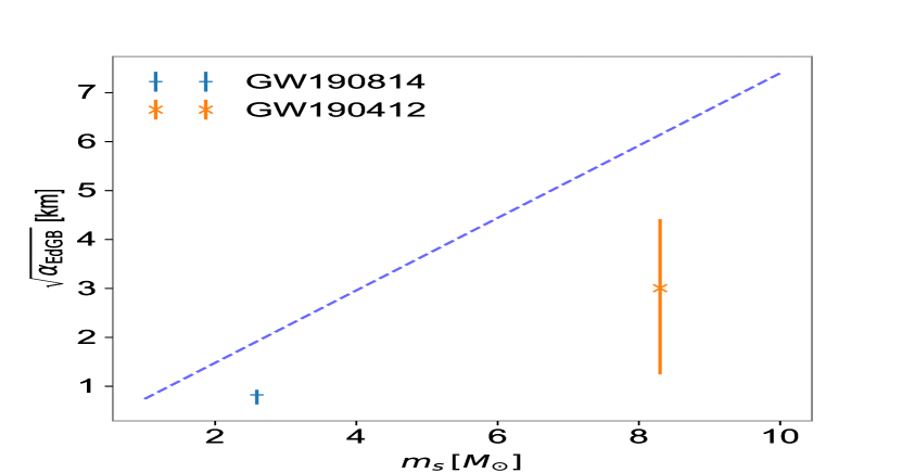
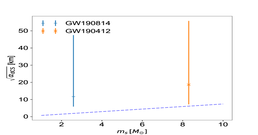
Figure 1: Reweighted results of $\sqrt{\alpha_{\rm EdGB}}$ (left panel) and $\sqrt{\alpha_{\rm dCS}}$ (right panel) for GW190412 and GW190814. The dashed lines are the relation between the median value of the secondary mass and the threshold value of $\sqrt{\alpha_{\rm EdGB,dCS}}$ given by Eq.(3). The secondary masses of GW190412 and GW190814 are $8.3^{+1.6}_{-0.9}M_{\odot}$ and $2.59^{+0.08}_{-0.09}M_{\odot}$ at $90\%$ credibility (Abbott et al., 2020a). Then the threshold values of $\sqrt{\alpha_{\rm EdGB,dCS}}$ are calculated with the median values of the secondary masses of these two events. The data points show the median values and $90\%$ regions of the $\sqrt{\alpha_{\rm EdGB,dCS}}$ posterior distributions. Evidently, both GW190814 and GW190412 can place meaningful constraints on $\sqrt{\alpha_{\rm EdGB}}$, and GW190814 works better than GW190412. However, both events are unable to place meaningful constraints on $\sqrt{\alpha_{\rm dCS}}$.

Recently, based on the general consideration about the stability of BHs in EdGB gravity (Witek et al., 2019), Carullo (2021) has obtained the most stringent constraint to date on EdGB, $\sqrt{\alpha_{\rm EdGB}}\lesssim 0.8\,\rm km$, by assuming the secondary object of GW190814 is a BH. The analysis based on inspiral data is different. The leading order of the scalar charge effect in EdGB gravity enters at $-1$ PN while the leading order of the tidal effect enters at $1$ PN (Vines et al., 2011; Damour et al., 2012), which means that the modification on the inspiral waveform keeps the original form in this theory. The only difference is $s^{\rm EdGB}=0$ for NS components. However, constraining the EdGB under the assumption that GW190814 is a NSBH is not feasible since there is no NSBH waveform model that includes both higher multipoles and precession effects. If these two effects are excluded, we cannot unbiasedly constrain the secondary mass of GW190814 as well (Abbott et al., 2020c), and then the constraints on EdGB and dCS gravity would be biased. Note that in the discussion below Eq.(2) we have presented some arguments for the BBH merger origin of GW190814.

Events	Methods	$\sqrt{\alpha_{\rm EdGB}}\,(\rm km)$
GW190412	Reweighting	$4.41$
	Bayes XPHM	$4.46$
GW190814	Reweighting	$0.93$
	Bayes XPHM	$0.40$
	Bayes Pv3HM	$0.38$

Table 1: Constraints on $\sqrt{\alpha_{\rm EdGB}}$ with reweighting and Bayesian analyses. The Bayesian analyses are performed with both the IMRPhenomPv3HM (Pv3HM) waveform model and the IMRPhenomXPHM (XPHM) waveform model. All constraints are presented as the upper limits for each individual event at $90\%$ credibility.

We further carry out Bayesian analyses on GW190412 and on GW190814, assuming they are BBH events, which give better constraints on both $\sqrt{\alpha_{\rm dCS}}$ and $\sqrt{\alpha_{\rm EdGB}}$ parameters. Among them, the posteriors of $\sqrt{\alpha_{\rm dCS}}$ are still not respecting the small-coupling conditions, and thus cannot place meaningful constraint on it. The comparison of constraints between the fully Bayesian and the reweighting analyses on $\sqrt{\alpha_{\rm EdGB}}$ is summarized in Table 1. In Fig. 2, we also show the posterior distributions of $\sqrt{\alpha_{\rm EdGB}}$, which are from the Bayesian and reweighting analyses of GW190412 and GW190814.

For GW190814, the Bayesian inferences are performed with both IMRPhenomPv3HM and IMRPhenomXPHM waveform models, resulting in similar constraints, $\sqrt{\alpha_{\rm EdGB}}\lesssim 0.40\,\rm km$ and $\sqrt{\alpha_{\rm EdGB}}\lesssim 0.38\,\rm km$ at $90\%$ credibility, respectively. The little difference between results of these two waveform models can be explained by the statistical noise. Thus, the difference between these two waveform models can be ignored in this work. On the other hand, the constraint from the reweighting analysis is $\sqrt{\alpha_{\rm EdGB}}\lesssim 0.93\,\rm km$ at $90\%$ credibility. The Bayesian-analyses-based constraints are tighter than that of the reweighting analysis by a factor of approximately $2$. Also, notice that more than $99\%$ of the posterior distributions of GW190412 and GW190814 from the reweighting analysis lies beyond $0$, which may mislead deviations from GR. Differences between the reweighting analysis and the Bayesian analysis are reasonable since the reweighting analysis does not take into account full correlations between parameters as the Bayesian analysis does. Strictly speaking, we employ resample points from the posterior distributions of parameters $(\delta\phi_{-2},m_{1},m_{2},\chi_{1},\chi_{2},\theta_{1},\theta_{2})$ individually in order to get the posterior of $\sqrt{\alpha_{\rm EdGB}}$, which may also lead to a biased posterior distribution on it.

For GW190412, the constraint from the Bayesian analysis is similar to that from the reweighting analysis at $90\%$ credibility, but the former performs better than the latter at $68.3\%$ credibility, $\sqrt{\alpha_{\rm EdGB}}\lesssim 2.46$ and $\sqrt{\alpha_{\rm EdGB}}\lesssim 3.53\,\rm km$ respectively. The constraint from the Bayesian analysis on GW190412 is not as stringent as that of GW190814, which is due to the shorter inspiral signal (lower SNR) and the smaller mass ratio (assuming $q>1$) of GW190412. Thus, the difference between results of a Bayesian analysis and the reweighting analysis is not as obvious as GW190814. The posterior distributions for all parameters of GW190412 and GW190814 are presented in Appendix. A.

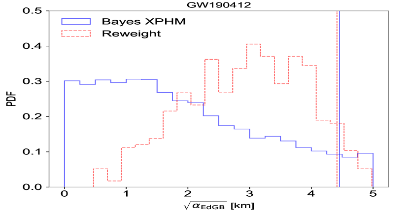
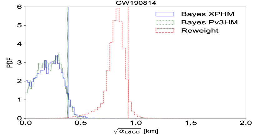
Figure 2: Probability density functions of $\sqrt{\alpha_{\rm EdGB}}$ for GW190412 (left panel) and GW190814 (right panel). For GW190412, the constraints of the Bayesian analysis performed with the IMRPhenomXPHM waveform model (solid histogram) and the reweighting analysis (dashed histogram) are $\sqrt{\alpha_{\rm EdGB}}\lesssim 4.46$ and $\sqrt{\alpha_{\rm EdGB}}\lesssim 4.41\,\rm km$, at $90\%$ credible level, respectively. For GW190814, the constraints from Bayesian inference with the IMRPhenomXPHM (solid histogram) waveform model is $\sqrt{\alpha_{\rm EdGB}}\lesssim 0.40\,\rm km$ at $90\%$ credibility. For GW190814, the constraints from Bayesian inference with both IMRPhenomXPHM (solid histogram) and IMRPhenomPv3HM (dotted histogram) waveform models are $\sqrt{\alpha_{\rm EdGB}}\lesssim 0.40$ and $\sqrt{\alpha_{\rm EdGB}}\lesssim 0.38\,\rm km$ at $90\%$ credible level, respectively. As a comparison, the reweighting analysis (dashed histogram) gives the constraint $\sqrt{\alpha_{\rm EdGB}}\lesssim 0.93\,\rm km$ at $90\%$ credibility. For both events, results of the reweighting analysis are biased, leading to evidence for deviation from GR. This is due to the absence of the correlations between parameters in this method.

IV Conclusions

In this work, we have tried to constrain the parameters of two typical theories alternative to GR, EdGB and dCS, $\sqrt{\alpha_{\rm EdGB,dCS}}$, by adopting two methods, i.e., the reweighting and full Bayesian analyses to analyze the two events of GWTC-2, GW190412, and GW190814. As expected, these two events in GWTC-2 cannot place constraints on the parameter $\sqrt{\alpha_{\rm dCS}}$. A $90\%$ bound of $\sqrt{\alpha_{\rm EdGB}}\lesssim 0.40\,\rm km$ is given by Bayesian analysis of GW190814, assuming it is a BBH merger. The constraint from Bayesian analysis of GW190412 is $\sqrt{\alpha_{\rm EdGB}}\lesssim 4.46\,\rm km$ at $90\%$ credibility. The Bayesian analyses give a stringent constraint on $\sqrt{\alpha_{\rm EdGB}}$, in agreement with GR, and this is different from the posterior distributions given by the reweighting analysis. The results of the reweighting analysis are biased, which may attribute to the fact that the reweighting analysis ignores the correlations between parameters.

Before this work, the most stringent constraint ($90\%$ credibility) is $\sqrt{\alpha_{\rm EdGB}}\lesssim 0.8\,\rm km$ (Carullo, 2021), which was obtained from the stability analysis of BHs in EdGB gravity. The constraint from GW190814 has improved it by a factor of about $2$. Note that the constraint presented by Carullo (2021) does not rely on a perturbative assumption, while our result does. In Ref. (Nair et al., 2019), a $90\%$ bound of $\sqrt{\alpha_{\rm EdGB}}\lesssim 5.6\,\rm km$ was reported by analyzing the GW events in GWTC-1. The fact that the constraints from GW190814 have been improved by about an order of magnitude is reasonable due to the presence of precession and higher multipoles, which will improve the estimation of masses and spins of the sources (Abbott et al., 2020d, c). From the fundamental physics side, the strongest constraint we have placed on EdGB gravity may strengthen the pillars of GR such as the strong equivalence principle and the no-hair theorem of black holes.

Appendix A Posterior distributions

In Figs.3 and 4, we show the posterior distributions for all parameters of GW190412 and GW190814, respectively. The ranges of these distributions are wider compared with that of full IMR analyses (Abbott et al., 2020a), which is due to the low-pass cutoff frequencies $f_{\rm high}$ used in analyses of GW190412 ($f_{\rm high}=83$ Hz) and GW190814 ($f_{\rm high}=137$ Hz).

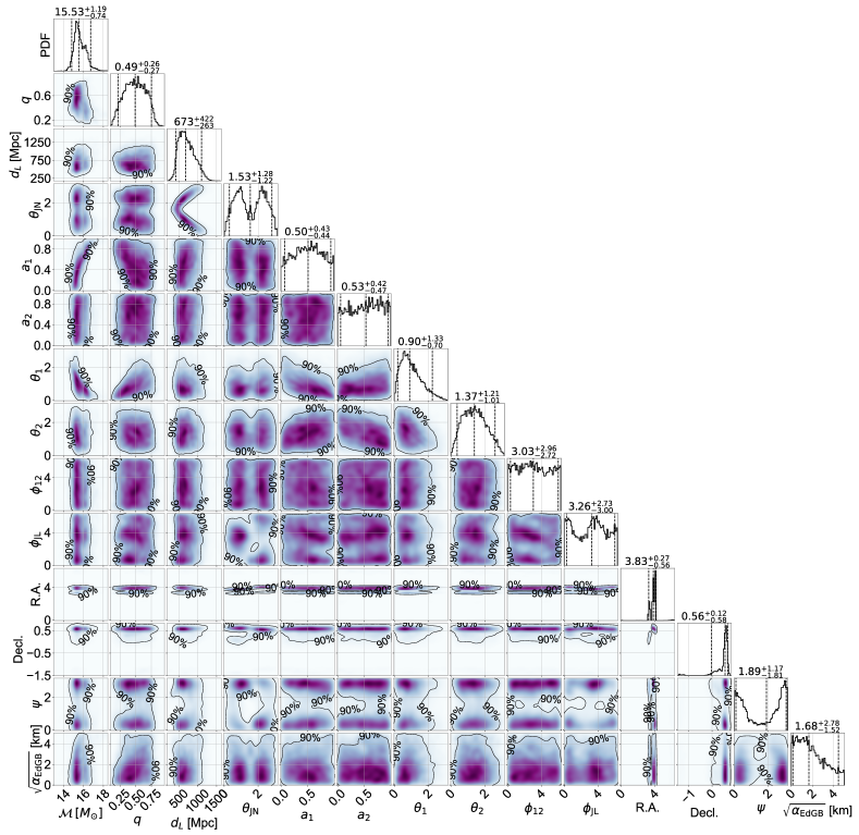
Figure 3: Posterior distributions for parameters of GW190412, analyzed with the IMRPhenomXPHM waveform model. The low-pass cutoff frequency $f_{\rm high}$ is $83$ Hz. The contours represent the credible level at $90\%$. The numbers listed in the diagonal are the median values and the $90\%$-credible measurements of each parameter.

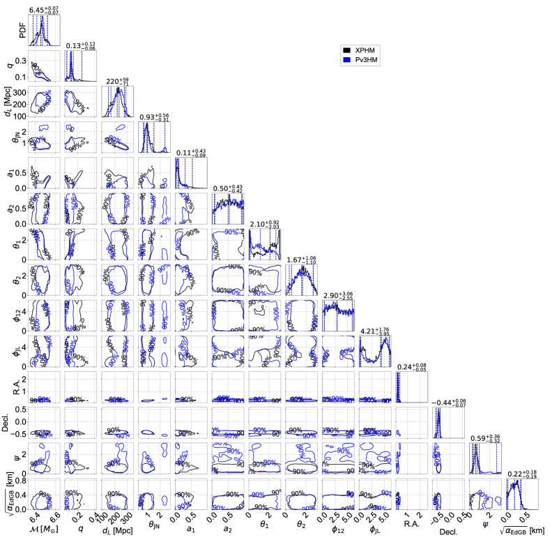
Figure 4: Posterior distributions for parameters of GW190814, analyzed with IMRPhenomXPHM and IMRPhenomPv3HM waveform models. The low-pass cutoff frequency $f_{\rm high}$ is $137$ Hz. The contours represent the credible level at $90\%$. The numbers listed in the diagonal are the median values and the $90\%$-credible measurements of each parameter of the IMRPhenomXPHM waveform model.

References

- Abbott et al. (2016) B. P. Abbott et al. (LIGO Scientific, Virgo), Phys. Rev. Lett. 116, 221101 (2016), [Erratum: Phys. Rev. Lett.121,no.12,129902(2018)], arXiv:1602.03841 [gr-qc] .
- Abbott et al. (2019a) B. P. Abbott, R. Abbott, and T. D. e. a. Abbott (LIGO Scientific Collaboration and Virgo Collaboration), Phys. Rev. Lett 123, 011102 (2019a), arXiv:1811.00364 [gr-qc] .
- Abbott et al. (2019b) B. P. Abbott, R. Abbott, and T. D. e. a. Abbott (The LIGO Scientific Collaboration and the Virgo Collaboration), Phys. Rev. D 100, 104036 (2019b).
- Abbott et al. (2020a) R. Abbott, T. D. Abbott, S. Abraham, F. Acernese, K. Ackley, A. Adams, C. Adams, R. X. Adhikari, V. B. Adya, C. Affeldt, and et al., arXiv e-prints , arXiv:2010.14527 (2020a), arXiv:2010.14527 [gr-qc] .
- Abbott et al. (2020b) R. Abbott, T. D. Abbott, S. Abraham, F. Acernese, K. Ackley, A. Adams, C. Adams, R. X. Adhikari, V. B. Adya, C. Affeldt, and et al., Astrophysical Journal, Letters 892, L3 (2020b), arXiv:2001.01761 [astro-ph.HE] .
- Han et al. (2020) M.-Z. Han, S.-P. Tang, Y.-M. Hu, Y.-J. Li, J.-L. Jiang, Z.-P. Jin, Y.-Z. Fan, and D.-M. Wei, Astrophysical Journal, Letters 891, L5 (2020), arXiv:2001.07882 [astro-ph.HE] .
- Abbott et al. (2020c) R. Abbott, T. D. Abbott, S. Abraham, F. Acernese, K. Ackley, A. Adams, C. Adams, R. X. Adhikari, V. B. Adya, C. Affeldt, and et al., Astrophysical Journal, Letters 896, L44 (2020c), arXiv:2006.12611 [astro-ph.HE] .
- Abbott et al. (2020d) R. Abbott, T. D. Abbott, S. Abraham, F. Acernese, K. Ackley, A. Adams, C. Adams, R. X. Adhikari, V. B. Adya, C. Affeldt, and et al., Phys. Rev. D 102, 043015 (2020d).
- Abbott et al. (2020e) R. Abbott, T. D. Abbott, S. Abraham, F. Acernese, K. Ackley, A. Adams, C. Adams, R. X. Adhikari, V. B. Adya, C. Affeldt, and et al., Astrophysical Journal, Letters 900, L13 (2020e), arXiv:2009.01190 [astro-ph.HE] .
- Abbott et al. (2020f) R. Abbott, T. D. Abbott, S. Abraham, F. Acernese, K. Ackley, A. Adams, C. Adams, R. X. Adhikari, V. B. Adya, C. Affeldt, and et al., Phys. Rev. Lett 125, 101102 (2020f), arXiv:2009.01075 [gr-qc] .
- Abbott et al. (2020) B. P. Abbott, R. Abbott, and T. D. e. a. Abbott (The LIGO Scientific Collaboration and the Virgo Collaboration), arXiv e-prints , arXiv:2010.14529 (2020), arXiv:2010.14529 [gr-qc] .
- Abbott et al. (2019c) B. P. Abbott, R. Abbott, and T. D. e. a. Abbott (LIGO Scientific Collaboration and Virgo Collaboration), Phys. Rev. X 9, 031040 (2019c).
- Witek et al. (2019) H. Witek, L. Gualtieri, P. Pani, and T. P. Sotiriou, Phys. Rev. D 99, 064035 (2019), arXiv:1810.05177 [gr-qc] .
- Okounkova et al. (2019) M. Okounkova, L. C. Stein, M. A. Scheel, and S. A. Teukolsky, Phys. Rev. D 100, 104026 (2019), arXiv:1906.08789 [gr-qc] .
- Okounkova (2020) M. Okounkova, Phys. Rev. D 102, 084046 (2020), arXiv:2001.03571 [gr-qc] .
- Blanchet (2014) L. Blanchet, Living Rev. Rel. 17, 2 (2014), arXiv:1310.1528 [gr-qc] .
- Kokkotas and Schmidt (1999) K. D. Kokkotas and B. G. Schmidt, Living Reviews in Relativity 2, 2 (1999), arXiv:gr-qc/9909058 [gr-qc] .
- Ferrari and Gualtieri (2008) V. Ferrari and L. Gualtieri, General Relativity and Gravitation 40, 945 (2008), arXiv:0709.0657 [gr-qc] .
- Berti et al. (2009) E. Berti, V. Cardoso, and A. O. Starinets, Classical and Quantum Gravity 26, 163001 (2009), arXiv:0905.2975 [gr-qc] .
- Yunes and Pretorius (2009) N. Yunes and F. Pretorius, Phys. Rev. D 80, 122003 (2009).
- Yunes et al. (2016) N. Yunes, K. Yagi, and F. Pretorius, Phys. Rev. D 94, 084002 (2016).
- Kanti et al. (1996) P. Kanti, N. E. Mavromatos, J. Rizos, K. Tamvakis, and E. Winstanley, Phys. Rev. D 54, 5049 (1996), arXiv:hep-th/9511071 [hep-th] .
- Yagi et al. (2016) K. Yagi, L. C. Stein, and N. Yunes, Phys. Rev. D 93, 024010 (2016), arXiv:1510.02152 [gr-qc] .
- Alexander and Yunes (2009) S. Alexander and N. Yunes, Physics Reports 480, 1 (2009), arXiv:0907.2562 [hep-th] .
- Nair et al. (2019) R. Nair, S. Perkins, H. O. Silva, and N. Yunes, Phys. Rev. Lett 123, 191101 (2019), arXiv:1905.00870 [gr-qc] .
- Khan et al. (2020) S. Khan, F. Ohme, K. Chatziioannou, and M. Hannam, Phys. Rev. D 101, 024056 (2020), arXiv:1911.06050 [gr-qc] .
- Yagi et al. (2012a) K. Yagi, L. C. Stein, N. Yunes, and T. Tanaka, Phys. Rev. D 85, 064022 (2012a), arXiv:1110.5950 [gr-qc] .
- Carson et al. (2020) Z. Carson, B. C. Seymour, and K. Yagi, Classical and Quantum Gravity 37, 065008 (2020), arXiv:1907.03897 [gr-qc] .
- Vines et al. (2011) J. Vines, É. É. Flanagan, and T. Hinderer, Phys. Rev. D 83, 084051 (2011), arXiv:1101.1673 [gr-qc] .
- Damour et al. (2012) T. Damour, A. Nagar, and L. Villain, Phys. Rev. D 85, 123007 (2012), arXiv:1203.4352 [gr-qc] .
- Tahura et al. (2019) S. Tahura, K. Yagi, and Z. Carson, Phys. Rev. D100, 104001 (2019), arXiv:1907.10059 [gr-qc] .
- Berti et al. (2018) E. Berti, K. Yagi, and N. Yunes, General Relativity and Gravitation 50, 46 (2018), arXiv:1801.03208 [gr-qc] .
- Prabhu and Stein (2018) K. Prabhu and L. C. Stein, Phys. Rev. D 98, 021503 (2018), arXiv:1805.02668 [gr-qc] .
- Yagi et al. (2012b) K. Yagi, N. Yunes, and T. Tanaka, Phys. Rev. Lett 109, 251105 (2012b), arXiv:1208.5102 [gr-qc] .
- Tahura and Yagi (2018) S. Tahura and K. Yagi, Phys. Rev. D 98, 084042 (2018), arXiv:1809.00259 [gr-qc] .
- Tews et al. (2021) I. Tews, P. T. H. Pang, T. Dietrich, M. W. Coughlin, S. Antier, M. Bulla, J. Heinzel, and L. Issa, Astrophysical Journal, Letters 908, L1 (2021), arXiv:2007.06057 [astro-ph.HE] .
- Nathanail et al. (2021) A. Nathanail, E. R. Most, and L. Rezzolla, Astrophysical Journal, Letters 908, L28 (2021), arXiv:2101.01735 [astro-ph.HE] .
- Shao et al. (2020) D.-S. Shao, S.-P. Tang, J.-L. Jiang, and Y.-Z. Fan, Phys. Rev. D 102, 063006 (2020), arXiv:2009.04275 [astro-ph.HE] .
- Veitch et al. (2015) J. Veitch, V. Raymond, B. Farr, W. Farr, P. Graff, S. Vitale, B. Aylott, K. Blackburn, N. Christensen, M. Coughlin, W. Del Pozzo, F. Feroz, J. Gair, C. J. Haster, V. Kalogera, T. Littenberg, I. Mandel, R. O’Shaughnessy, M. Pitkin, C. Rodriguez, C. Röver, T. Sidery, R. Smith, M. Van Der Sluys, A. Vecchio, W. Vousden, and L. Wade, Phys. Rev. D 91, 042003 (2015), arXiv:1409.7215 [gr-qc] .
- Khan et al. (2016) S. Khan, S. Husa, M. Hannam, F. Ohme, M. Pürrer, X. J. Forteza, and A. Bohé, Phys. Rev. D 93, 044007 (2016), arXiv:1508.07253 [gr-qc] .
- Ashton et al. (2019) G. Ashton, M. Hübner, P. D. Lasky, C. Talbot, K. Ackley, S. Biscoveanu, Q. Chu, A. Divakarla, P. J. Easter, B. Goncharov, F. H. Vivanco, J. Harms, M. E. Lower, G. D. Meadors, D. Melchor, E. Payne, M. D. Pitkin, J. Powell, N. Sarin, R. J. E. Smith, and E. Thrane, The Astrophysical Journal Supplement Series 241, 27 (2019).
- Speagle (2020) J. S. Speagle, MNRAS 493, 3132 (2020), arXiv:1904.02180 [astro-ph.IM] .
- Pratten et al. (2020) G. Pratten, C. García-Quirós, M. Colleoni, A. Ramos-Buades, H. Estellés, M. Mateu-Lucena, R. Jaume, M. Haney, D. Keitel, J. E. Thompson, and S. Husa, arXiv e-prints , arXiv:2004.06503 (2020), arXiv:2004.06503 [gr-qc] .
- Carullo (2021) G. Carullo, arXiv e-prints , arXiv:2102.05939 (2021), arXiv:2102.05939 [gr-qc] .