Two Particles with Zero-Range Interaction in a Magnetic Field

Abstract

Energy levels are investigated for two charged particles possessing an attractive, momentum-independent, zero-range interaction in a uniform magnetic field. A transcendental equation governs the spectrum, which is characterized by a collective Landau-level quantum number incorporating both center-of-mass and relative degrees of freedom. Results are obtained for a system of one charged and one neutral particle, with the interaction chosen to produce a bound state in vanishing magnetic field. Beyond deriving the weak-field expansion of the energy levels, we focus on non-perturbative aspects. In the strong-field limit, or equivalently for a system in the unitary limit, a single bound level with universal binding energy exists. By contrast, excited states are resonances that disappear into the continuum as the magnetic field is raised beyond critical values. A hyperbola is derived that approximates the number of bound levels as a function of the field strength remarkably well.

I Introductory Remarks

The study of quantum systems in external fields is central to many disciplines, with applications ranging from the study of ultracold gases of trapped atoms [1] to quantum field theories in condensed matter, nuclear, and particle physics [2]. In numerical gauge-theory calculations, external fields present a practical computational method to study properties of light nuclei using lattice quantum chromodynamics (LQCD). For an overview, see [3, 4, 5] and references therein. The first LQCD results for light nuclei in external magnetic fields [6, 7, 8] point to an intriguing possibility. The energies of a subset of two-nucleon systems in large magnetic fields appear to approach binding thresholds, which suggests an analogue of a Feshbach resonance [9, 10, 11]. While such resonances are extensively studied in atomic systems [12], the LQCD results hint at a similar effect in two-nucleon systems. The magnetic field, moreover, could provide a lever with which to tune two-nucleon systems simultaneously to threshold, arriving at a point of conformal symmetry [13].

Unlike atomic systems, the magnetic fields required to alter strongly interacting systems are exceptionally large, ${\mathcal{O}}(10^{19})$ Gauss. Fields of this size are routine in LQCD computations, due to quantization conditions required of uniform fields on a torus [14]. In astrophysics, strong magnetic fields have been conjectured to occur in the interiors of magnetars [15, 16, 17]. Such extreme fields, have been estimated to exist in non-central heavy-ion collisions [18, 19], moreover, for which considerable work has explored the implications for QCD matter [20].

In the present work, we investigate a two-body problem in uniform magnetic fields. For atomic systems, there is substantial work on Coulomb interactions in an external magnetic field, e.g. [21]. The analogous study of QCD bound states has begun recently; examples include quarkonium in external magnetic fields [22, 23], as well as modification of the quark-antiquark potential computed from LQCD [24]. For two protons in a magnetic field, the center-of-mass and relative motion can be separated. In this system, the effect of a sufficiently large magnetic field has been proven to result in a bound di-proton state [25]. The argument hinges on magnetic confinement of the protons into narrow cyclotron orbits. In such a scenario, the short-range nuclear interaction results in an attractive one-dimensional potential well, which always supports a bound state. To address the neutron-proton system in magnetic fields, however, one needs to confront the non-separability of the center-of-mass and relative degrees of freedom, and we take a first step in this work.

General results for charged particles with translationally invariant interactions in a magnetic field were established in [27]. In particular, a quantum number exists that collectively incorporates the center-of-mass and relative degrees of freedom, and each level is infinitely degenerate. This provides a striking generalization of the Landau problem to all values of the magnetic field. We exhibit these results by solving for the energy levels of two charged particles interacting with a contact potential. The choice of an attractive, momentum-independent, zero-range interaction is motivated by the pion-less effective theory of few-nucleon systems [28, 29, 30, 31]. The zero-range interaction between particles produces valuable simplifications that facilitate determining the spectrum. The energies of this system are found to obey a transcendental equation; moreover, through a judicious form of renormalization, the inverse solution (magnetic field as a function of energy) is obtained simply by quadrature.

We begin our treatment with a general discussion in Sec. II, where we exhibit the quantum number incorporating both center-of-mass and relative degrees of freedom. In Sec. III, we focus on a system consisting of one charged and one neutral particle, for which the spectrum is obtained as a function of the magnetic field. Perturbative expansions are derived about the small-field and unitary limits. The number of bound levels supported as a function of the magnetic field is shown to obey a simple equation. A summary of results is given in Sec. IV, while various technical details are provided in Apps. A and B.

II General Discussion

The system under consideration is that of two particles with charges $q_{a}$ and masses $m_{a}$, where $a=1$, $2$. The particles are in a uniform magnetic field and interact through an attractive, zero-range potential in three spatial dimensions. The Hamiltonian for this system has the form

$$H=H^{(0)}-c\,{\delta}(\bm{r}),$$ (1)

where $\bm{r}={\bm{r}}_{1}-{\bm{r}}_{2}$ is the relative coordinate between the particles. Without the two-body potential, the Hamiltonian for two particles in a magnetic field is additive

$$H^{(0)}=\sum_{a=1}^{2}H^{(0)}_{a}=\sum_{a=1}^{2}\frac{\big{[}{\bm{p}}_{a}-q_{a}{\bm{A}}({\bm{r}}_{a})\big{]}^{2}}{2m_{a}},$$ (2)

where ${\bm{A}}$ is the vector potential that specifies the magnetic field. For arbitrary values of the charges and masses of the two particles, there is no general separation between the relative and center-of-mass motion. At the quantum level, the eigenvalues of $H$ are neither the sum of relative and center-of-mass contributions, nor are they the sum of single-particle contributions.

A bound state with energy ${\mathcal{E}}$ appears as a solution to the homogeneous Lippmann-Schwinger integral equation

$$\Psi({\bm{r}}_{1},{\bm{r}}_{2})=-c\int d{\bm{R}}\,G^{(0)}({\bm{r}}_{1},{\bm{r}}_{2};{\bm{R}},{\bm{R}}|{\mathcal{E}})\Psi({\bm{R}},{\bm{R}}),\,\,$$ (3)

where $G^{(0)}$ is the non-interacting two-particle Green’s function

$$G^{(0)}({\bm{r}}^{\prime}_{1},{\bm{r}}^{\prime}_{2};{\bm{r}}_{1},{\bm{r}}_{2}|{\mathcal{E}})=\big{\langle}{\bm{r}}^{\prime}_{1},{\bm{r}}^{\prime}_{2}\big{|}\frac{1}{{\mathcal{E}}-H^{(0)}+i{\epsilon}}\big{|}{\bm{r}}_{1},{\bm{r}}_{2}\big{\rangle},\quad\,\,\,$$ (4)

and the integration is over the center-of-mass coordinate ${\bm{R}}$. By virtue of the contact potential, the integration over the relative separation amounts to an evaluation of the wave-function in the integrand at $\bm{r}=0$. While center-of-mass and relative coordinates are not completely decoupled in $H^{(0)}$, partial factorization of the wave-function is possible. Assuming a non-vanishing charge for the system $Q\equiv q_{1}+q_{2}$, the center-of-mass wave-function is specified by the momentum parallel to the magnetic field, along with one other quantum number. This quantum number can be chosen as an additional component of the total momentum, for which the asymmetric gauge is natural. Therefore, we adopt

$${\bm{A}}({\bm{r}})=\left(-By,0,0\right),$$ (5)

leading to the magnetic field ${\bm{B}}=B\bm{\hat{z}}$. Accordingly, the $x$- and $z$-components of the total momentum ${\bm{P}}={\bm{p}}_{1}+{\bm{p}}_{2}$, are good quantum numbers. For any vector ${\bm{v}}$, we define a related vector $\bm{\widetilde{v}}$, with two non-vanishing components $\bm{\widetilde{v}}=\left(v_{x},0,v_{z}\right)$, so that, e.g., $\bm{\widetilde{P}}$ refers to the good components of ${\bm{P}}$.

The two-particle wave-function can be written in the partially factorized form

$$\Psi({\bm{r}}_{1},{\bm{r}}_{2})=e^{i\bm{\widetilde{P}}\cdot\bm{\widetilde{R}}}\,\,\Psi_{P_{x}}(Y,\bm{r}),$$ (6)

in which $\Psi_{P_{x}}(Y,\bm{r})$ reflects the coupled center-of-mass and relative motion. The $\bm{\widetilde{P}}$-projected non-interacting Green’s function is obtained through the Fourier decomposition

$$G^{(0)}({\bm{r}}^{\prime}_{1},{\bm{r}}^{\prime}_{2};{\bm{r}}_{1},{\bm{r}}_{2}|{\mathcal{E}}) = \int\frac{d\bm{\widetilde{P}}}{(2{\pi})^{2}}\,e^{i\bm{\widetilde{P}}\cdot\left(\bm{\widetilde{R}}^{\prime}-\bm{\widetilde{R}}\right)}\qquad\qquad$$ (7)

$$\phantom{sp}\times G^{(0)}_{P_{x}}(Y^{\prime},\bm{r}^{\prime};Y,\bm{r}|E),\,\,$$

where the shifted energy $E={\mathcal{E}}-\frac{P_{z}^{2}}{2M}$ serves to remove all $P_{z}$-dependence from the projected Green’s function. Projecting Eq. (3) onto states of good $\bm{\widetilde{P}}$, leads to the wave equation

$$\Psi_{P_{x}}(Y,\bm{r})=-c\int dY^{\prime}G^{(0)}_{P_{x}}(Y,\bm{r};Y^{\prime},{\bm{0}}|E)\Psi_{P_{x}}(Y^{\prime},{\bm{0}}).\quad\,\,\,$$ (8)

As with Eq. (3), the wave-function appearing in the integrand is evaluated at zero relative separation owing to the contact interaction. Knowledge of this restricted wave-function $\Psi_{P_{x}}(Y^{\prime},{\bm{0}})$ thus determines the value for $\bm{r}\neq{\bm{0}}$ by convolution with the non-interacting Green’s function.

The restricted equation

$$\Psi_{P_{x}}(Y,{\bm{0}})=-c\int dY^{\prime}G^{(0)}_{P_{x}}(Y,{\bm{0}};Y^{\prime},{\bm{0}}|E)\Psi_{P_{x}}(Y^{\prime},{\bm{0}}),\quad\quad$$ (9)

is obtained by evaluating Eq. (8) at $\bm{r}={\bm{0}}$, and suffices to determine the energy $E$. Simplifications arise because the configuration space is restricted to both particles being at the same point, for which there remains only center-of-mass motion of a system having charge $Q$. This is manifest in the functional form of the restricted non-interacting Green’s function

$$G^{(0)}_{P_{x}}(Y,{\bm{0}};Y^{\prime},{\bm{0}}|E)=\sqrt{QB}\,\,g^{(0)}({\xi};{\xi}^{\prime}|E),$$ (10)

which has a simple form in terms of the dimensionless center-of-mass coordinates

$${\xi}=\sqrt{QB}\,(Y-Y_{0})\quad\text{and}\quad{\xi}^{\prime}=\sqrt{QB}\,(Y^{\prime}-Y_{0}),$$ (11)

where $Y_{0}=\frac{P_{x}}{QB}$ is the $y$-coordinate of the center of cyclotron motion of the restricted system. Written as a function of the variables ${\xi}$ and ${\xi}^{\prime}$, the restricted Green’s function $g^{(0)}$ has no dependence on $P_{x}$. Consequently, the energy determined from Eq. (9) is independent of $P_{x}$, which confirms that each $E$ is infinitely degenerate.

For arbitrary charges and masses of the two particles, explicit computation establishes that $g^{(0)}$ is diagonal in the basis of Hermite functions

$$g^{(0)}({\xi};{\xi}^{\prime}|E)=\sum_{n=0}^{\infty}g^{(0)}_{n}(E)\,\psi_{n}({\xi})\,\psi_{n}({\xi}^{\prime}).$$ (12)

Projecting Eq. (9) onto the $n$-th Hermite function, we obtain the equation

$$\frac{1}{c}+g^{(0)}_{n}(E)=0,$$ (13)

that determines $E$ for each value of $n$. This quantum number is the Landau level of the center of mass only when the two particles are restricted to the same point. With $\bm{r}\neq{\bm{0}}$, the Green’s function $G^{(0)}_{P_{x}}(Y,\bm{r};Y^{\prime},{\bm{0}}|E)$ is not diagonal in the basis of Hermite functions; accordingly, factorization of $\Psi_{P_{x}}(Y,\bm{r})$ does not result from Eq. (8). This reflects that the quantum number $n$ incorporates collective behavior of both center-of-mass and relative degrees of freedom.

III Determining the Energies:
An Example

As an example, we solve for the spectrum of a system consisting of one charged and one neutral particle. Accordingly, we take $q_{1}=Q$ and $q_{2}=0$. To exhibit various properties of the solution, we keep the masses $m_{1}$ and $m_{2}$ different.

III.1 Equations for the Spectrum

For this system, computation of the restricted, non-interacting Green’s function, Eq. (10), is detailed in App. A. The calculation produces the coefficients $g_{n}^{(0)}(E)$ of Eq. (12) expressed in terms of a Laplace transform. The equation for the bound-state energy, Eq. (13), thus takes the form

$$\frac{1}{c(t_{0})}-\int_{t_{0}}^{\infty}dt\,e^{Et}\,g^{(0)}_{n}(t)=0,$$ (14)

where we introduce a small-time cutoff $t_{0}$ to regulate the divergence at $t=0$. In Eq. (14), the coefficients are

$$g^{(0)}_{n}(t) = \left(\frac{{\mu}}{2\pi t}\right)^{\frac{3}{2}}\frac{M}{m_{1}}\,\frac{\sinh\frac{\Omega(t)\,t}{2}}{\sinh\frac{{\omega}t}{2}}\,e^{-\left(n+\frac{1}{2}\right){\Omega}(t)\,t},$$ (15)

and have been written in terms of the charged particle’s cyclotron frequency ${\omega}=QB/m_{1}$, as well as a time-dependent frequency $\Omega(t)$ defined through the relation

$$\coth\frac{{\Omega}(t)\,t}{2}=\coth\frac{{\omega}t}{2}+\frac{m_{2}}{m_{1}}\left(\frac{{\omega}t}{2}\right)^{-1}.$$ (16)

This time-dependent frequency is a curious feature governing the restricted cyclotron motion of the center of mass.

To renormalize Eq. (14), we inspect the small-time behavior of the integrand. In this limit, there is no magnetic field dependence, and we find the zero-field result

$$\frac{1}{c(t_{0})}-\int_{t_{0}}^{\infty}dt\,e^{E_{0}t}\left(\frac{{\mu}}{2\pi t}\right)^{\frac{3}{2}}=0,$$ (17)

where $E_{0}<0$ denotes the energy in zero magnetic field. The $t_{0}\to 0$ divergence of the integral in Eq. (14) thus subtracts the identical divergence in $\frac{1}{c(t_{0})}$. A renormalized form of Eq. (14) defined for $t_{0}=0$ is therefore

$$\int_{0}^{\infty}dt\left[e^{Et}\,g^{(0)}_{n}(t)-e^{E_{0}t}\left(\frac{{\mu}}{2\pi t}\right)^{\frac{3}{2}}\right]=0.$$ (18)

Any real energy $E$ below the two-particle dissociation threshold, see Eq. (22), that solves this equation corresponds to an infinitely degenerate bound state with quantum number $n$. Below, we utilize this equation to obtain the small-field expansion.

An alternate equation for the spectrum is obtained by realizing that Eq. (17) can be rewritten as

$$\frac{1}{c(t_{0})}-\int_{t_{0}}^{\infty}dt\,e^{Et}\left(\frac{{\mu}}{2{\pi}t}\right)^{\frac{3}{2}}=\frac{{\mu}}{2{\pi}}\left[\sqrt{-2{\mu}E}-\sqrt{-2{\mu}E_{0}}\right]$$

(19)

with $E$ corresponding to a general energy, and small $t_{0}$ understood for the integral. Using Eq. (19) for the running coupling, the renormalized and analytically continued equation for the energy $E$ can be cast in the form

$$b^{-\frac{1}{2}}={\mathcal{I}}_{n}(\chi,x),\quad$$ (20)

where the function ${\mathcal{I}}_{n}(\chi,x)$ is defined in App. B. Appearing above, $x$ is the mass ratio $x=m_{1}/M$, the magnetic field in dimensionless units is defined as

$$b=\frac{QB}{-2{\mu}E_{0}},$$ (21)

and the energy $E$ is written in terms of $\chi(b)$ in the form

$$E=\frac{{\omega}}{2}-\chi\frac{QB}{2\mu}.$$ (22)

This parametrization of the energy accounts for the fact that the threshold for two-particle decay is set by the energy of the lowest Landau level of the charged particle. With the sign of the second term in Eq. (22), $\chi$ is the binding energy in units of $\frac{QB}{2\mu}$. Notice that Eq. (20) readily gives the inverse function $b(\chi)$ by simply evaluating ${\mathcal{I}}_{n}(\chi,x)$, which is a one-dimensional integral. In accordance with regularization independence, the energies determined numerically from Eqs. (18) and (20) agree.

III.2 Small-Field Limit

For small magnetic fields, one can treat ${\omega}t\ll 1$, for which the time-dependent frequency in Eq. (16) becomes approximately time independent and equal to the cyclotron frequency ${\Omega}$ of the center of mass

$${\Omega}(t)\approx\frac{QB}{M}\equiv{\Omega}.$$ (23)

Retaining only this linear magnetic field dependence, the equation for the energies, Eq. (18), becomes

$$\int_{0}^{\infty}\frac{dt}{t^{3/2}}\left(e^{\left[E-(n+\frac{1}{2}){\Omega}\right]t}-e^{E_{0}t}\right)=0,$$ (24)

and leads to the requirement $E=E_{0}+(n+\frac{1}{2}){\Omega}$. For small magnetic fields, the energies are ordinary Landau levels of the center of mass.

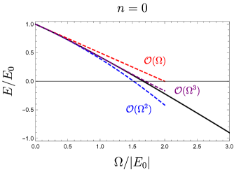
Figure 1: Behavior of the lowest level in small magnetic fields. For the case of equal masses, the ratio of the $n{=}0$ energy level $E$ to that in vanishing magnetic field $E_{0}$ is plotted (solid curve) as a function of the magnetic field, using the center-of-mass cyclotron frequency $\Omega$ in Eq. (23). Also plotted (dashed curves) are the perturbative approximations in powers of $\Omega/E_{0}$ from Eq. (25). While the state becomes less bound, note that $E=0$ does not correspond to threshold, see Eq. (22).

To obtain corrections to the leading-order result in small fields, we write ${\Delta}E=E-\left[E_{0}+(n+\frac{1}{2}){\Omega}\right]$, and iteratively solve for ${\Delta}E$ using Eq. (18). To third-order in the magnetic field, we find

$$E = E_{0}\Big{[}1+\Big{(}n+\frac{1}{2}\Big{)}\frac{{\Omega}}{E_{0}}-\frac{1}{48}\Big{(}4+\frac{m_{2}}{m_{1}}\Big{)}\frac{m_{2}}{m_{1}}\Big{(}\frac{{\Omega}}{E_{0}}\Big{)}^{2}$$ (25)

$$\phantom{sp}-\frac{1}{16}\Big{(}n+\frac{1}{2}\Big{)}\frac{m_{2}}{m_{1}}\Big{(}\frac{{\Omega}}{E_{0}}\Big{)}^{3}+{\mathcal{O}}(B^{4})\Big{]}.$$

In particular, the term at second order is independent of the quantum number $n$, and allows us to identify the magnetic polarizability of the bound state. Using the customary definition of the second-order energy shift ${\Delta}E=-\frac{1}{2}4{\pi}{\beta}_{M}B^{2}+\cdots$, we obtain the polarizability

$${\beta}_{M}=\frac{{\alpha}}{24}\left(4+\frac{m_{2}}{m_{1}}\right)\frac{m_{2}}{m_{1}}\,\frac{(Q/e)^{2}}{E_{0}M^{2}},$$ (26)

where ${\alpha}=e^{2}/4{\pi}$ is the fine-structure constant. The magnetic polarizability is diamagnetic ${\beta}_{M}<0$, due to the absence of paramagnetic spin contributions.

In Fig. 1, we exhibit the small-field behavior of the $n=0$ energy level determined from Eq. (20). For simplicity, we take the equal mass case $m_{1}=m_{2}$. Additionally shown is the small-field behavior determined analytically from Eq. (25). The perturbative expansion lines up well with the numerically determined energy, and appears to work beyond the $\Omega/|E_{0}|\ll 1$ regime.

III.3 Unitary Limit

To determine the behavior of the binding energy in the unitary limit $E_{0}\to 0$, we turn to Eq. (20). With $b\gg 1$, the binding energy in the unitary limit $\chi^{(0)}_{\infty}$ is obtained as the root of the equation

$${\mathcal{I}}_{n}(\infty)\equiv{\mathcal{I}}_{n}\Big{(}\chi^{(0)}_{\infty},x\Big{)}=0.$$ (27)

For $n>0$, there are no roots; only the $n{=}0$ level is bound for a system at unitarity. The binding energy in this regime, moreover, is independent of the short-range structure of the interaction. The bound state is thus a universal feature, albeit, in a limited sense. In dimensionless units, the unitary-limit binding energy still depends upon the mass ratio between the charged and neutral particles. This mass-ratio dependence is a consequence of the coupling between relative and center-of-mass motion. For identical masses ($x{=}\tfrac{1}{2}$), we obtain the numerical value $\chi^{(0)}_{\infty}=0.081588$. Only when the charged particle is much more massive than the neutral one ($x{\to}1$) does the system become unbound $\chi^{(0)}_{\infty}=0$. In the opposite limit, the binding energy of a system with a relatively light charge ($x{\to}0$) attains, by contrast, its largest value $\chi_{\infty}^{(0)}=0.605444$, which is twice the root of the Hurwitz zeta-function, see Eq. (39). Curiously, this value also appears as the binding energy of the spin-zero di-proton system in a strong magnetic field [25]. In other words, a single charge that interacts resonantly with a fixed force center (our model for $x{\to}0$) has the same ground-state energy as two particles with equal charge-to-mass ratios that interact via long-range Coulomb repulsion in addition to the zero-range attraction.

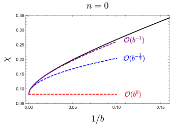
Figure 2: Behavior of the lowest level near unitarity. For the case of equal masses, $\chi$, the binding energy in units of $\frac{QB}{2{\mu}}$, is plotted (solid curve) as a function of the inverse magnetic field, using $b$ defined in Eq. (21). Also plotted (dashed curves) are the successive approximations in Eq. (28) about the unitary limit $b\gg 1$. For this level, the threshold $\chi{=}0$ is never reached.

Away from unitarity, the binding energy is no longer universal as it depends on $E_{0}$ through the $b^{-\frac{1}{2}}$ corrections. To obtain these corrections, we write the binding energy in the expansion

$$\chi=\chi^{(0)}_{\infty}+\frac{1}{\sqrt{b}}\,\chi^{(1)}_{\infty}+\frac{1}{b}\,\chi^{(2)}_{\infty}+{\mathcal{O}}\big{(}b^{-\frac{3}{2}}\big{)},$$ (28)

and then solve for the higher-order terms using Eq. (20) iteratively. This procedure results in

$$\chi^{(1)}_{\infty} = 1\Big{/}{\mathcal{I}}^{\prime}_{0}(\infty)=0.388235,$$

$$\chi^{(2)}_{\infty} = -\tfrac{1}{2}\,{\mathcal{I}}^{\prime\prime}_{0}(\infty)\Big{/}[{\mathcal{I}}^{\prime}_{0}(\infty)]^{3}=0.567853,\quad$$ (29)

where derivatives of ${\mathcal{I}}_{n}(\chi,x)$ are with respect to $\chi$, and the evaluation is at the location of the root in Eq. (27), namely at $\chi=\chi^{(0)}_{\infty}$. The formulas apply to any mass ratio, however, the numerical values quoted are exclusively for the equal-mass case ($x{=}\frac{1}{2}$). As the corrections away from unitarity are positive, the magnetic field always increases the ground-state binding energy and thus does not allow crossing to a virtual state.

In Fig. 2, we show the approach to unitarity of the $n=0$ energy level determined from Eq. (20). For simplicity, we again take the equal-mass case. Additionally shown is the behavior near the unitary limit obtained from Eq. (28), which does well in describing the magnetic-field dependence of the lowest energy level in this regime.

III.4 Binding Thresholds and the Number of Levels

The binding threshold is reached when $\chi{=}0$. As remarked above, the lowest level does not reach threshold; it remains bound in the unitary limit, which can alternately be viewed as the large-field limit with $E_{0}$ held fixed. The excited levels, however, reach threshold at critical values of the magnetic field. According to Eq. (20), the threshold for single-particle production occurs when the magnetic field has the value

$$b_{c}=\big{[}{\mathcal{I}}_{n}(0,x)\big{]}^{-2},$$ (30)

provided ${\mathcal{I}}_{n}(0,x)>0$. For the first excited level and with equal masses for the particles, we find

$$b_{c}=3.87554,\,\,\,\text{for}\,\,n{=}1\,\,\text{and}\,\,x{=}\tfrac{1}{2}.$$ (31)

For the higher-lying levels, the critical value of the magnetic field decreases monotonically. Consequently, we have the single-particle decay threshold at $b_{c}\ll 1$, for $n\gg 1$. Viewed as a function of the level number $n$, the critical field $b_{c}(n)$ can be obtained analytically in the large-$n$ limit. The analysis detailed in App. B produces the approximate formula

$$b_{c}=\frac{4}{2n-1}\left[1+{\mathcal{O}}(n^{-2})\right],$$ (32)

for the equal mass case. Surprisingly, the formula works at $3\%$ already for the $n{=}1$ level. Results improve with increasing $n$; the approximate critical field for $n{=}2$ differs by $0.6\%$ from the exact value.

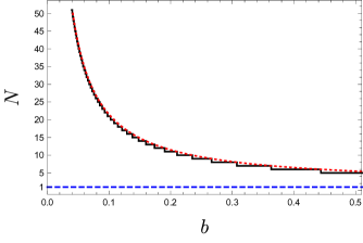
Figure 3: For the case of equal masses, the number of energy levels $N$ is plotted (solid curve) versus the magnetic field $b$ in Eq. (21). Each step down is due to a level reaching the binding threshold. The ground level never reaches the single-particle decay threshold, for which a horizontal dashed line depicts the large-$b$ value $N=1$. Additionally shown (dashed curve) is the approximate function $N(b)$ given in Eq. (33).

The number of energy levels supported in a given magnetic field can be obtained from knowledge of the critical field for each value of $n$. If we start at large $b$, the number of levels is $N=1$ until the field is lowered below the value in Eq. (31). Below this value, the $n{=}1$ level has not crossed threshold, consequently $N=2$. Continuing to lower the magnetic field, successive critical fields will be crossed and the number of levels increased by one each time. The number of levels obtained by counting thresholds is shown in Fig. 3 up to $N=50$. By identifying $N=n+1$ and simply inverting the formula for the critical field Eq. (32), we obtain an approximate formula for the number of levels as a function of the magnetic field

$$N=\tfrac{2}{b}+\tfrac{3}{2}.$$ (33)

The figure shows that this simple formula accounts for the number of bound levels remarkably well.

IV Summary

Systems of two interacting charged particles in a magnetic field present an analytically challenging non-separable problem. When the particles have an attractive, momentum-independent, zero-range interaction, we confirm in Sec. II that the bound states have infinite degeneracy, and are characterized by a quantum number that incorporates both center-of-mass and relative degrees of freedom. In small magnetic fields, this quantum number is the Landau level of the center of mass, as exhibited by Eq. (25), which is the small-field expansion of the energy of a system consisting of one charged and one neutral particle. Near the unitary limit, there is dramatically different behavior for the ground and excited levels of this system. The lowest level is bound, with a universal binding energy determined by Eq. (27). The excited states disappear into the continuum at critical values of the magnetic field, which are determined by Eq. (30). The number of bound levels as a function of the magnetic field is well described by the remarkably simple formula in Eq. (33).

A striking feature of this two-body system in a magnetic background is that its bound-state spectrum is identical to that of an effective one-body problem. The effective interaction in this restricted space accounts for the background field and zero-range interaction. The closed-form correlation function, Eq. (15), is suggestive of an effective time-dependent Hamiltonian. In this way, complexity of the non-separable system manifests as non-trivial time-dependence of the restricted system. Nonetheless, renormalization can be carried out by hand, thus enabling straightforward determination of spectral properties. In particular, Eq. (20) shows that the inverse of the solution, namely the magnetic field as a function of the binding energy, only requires evaluation of a one-dimensional integral. The number of systems possessing such almost-in-closed-form solutions can be enlarged by generalizing and extending the problem solved here. Of particular interest would be a complete treatment of the two-nucleon system.

Appendix A Green’s Function

The Green’s function $G^{(0)}$ in Eq. (4) is computed from a Laplace transform using the inverse operator

$$\frac{1}{E-H^{(0)}+i{\epsilon}}=-\int_{0}^{\infty}dt\,e^{Et}\,e^{-H^{(0)}t},$$ (34)

where analytic continuation is necessary when $E>0$. We refer to $t$ as time; although, strictly speaking, it is imaginary time. As $H^{(0)}_{1}$ and $H^{(0)}_{2}$ in Eq. (2) commute, $G^{(0)}$ factorizes into the product of single-particle Green’s functions

$$G^{(0)}({\bm{r}}^{\prime}_{1},{\bm{r}}^{\prime}_{2};{\bm{r}}_{1},{\bm{r}}_{2}|t) = \prod_{a=1}^{2}\,\big{\langle}{\bm{r}}^{\prime}_{a}\big{|}e^{-H^{(0)}_{a}t}\big{|}{\bm{r}}_{a}\big{\rangle}.$$ (35)

For the gauge chosen in Eq. (5), the Green’s function of the charged particle takes the form

$$\big{\langle}{\bm{r}}^{\prime}_{1}\big{|}e^{-H^{(0)}_{1}t}\big{|}{\bm{r}}_{1}\big{\rangle} = \int\frac{d\bm{\tilde{p}}_{1}}{(2\pi)^{2}}e^{i\bm{\tilde{p}}_{1}\cdot(\bm{\tilde{r}}^{\prime}_{1}-\bm{\tilde{r}}_{1})}e^{-\frac{p_{1,z}^{2}}{2m_{1}}t}$$ (36)

$$\qquad\times\sqrt{QB}\,\,\big{\langle}{\xi}^{\prime}_{1},\,{\omega}t\,\big{|}{\xi}_{1},0\big{\rangle},$$

and has been written in terms of the Green’s function of the simple harmonic oscillator. With dimensionless conjugate variables ${\xi}$ and $p_{\xi}$, the oscillator Hamiltonian appears as ${\mathcal{H}}=\frac{1}{2}\big{(}p_{\xi}^{2}+{\xi}^{2}\big{)}$, for which the corresponding propagator we define as $\langle{\xi}^{\prime},s\,|{\xi},0\rangle=\langle{\xi}^{\prime}|e^{-{\mathcal{H}}\,s}|{\xi}\rangle$. In Eq. (36), ${\omega}$ is the charged particle’s cyclotron frequency, and the dimensionless charged-particle coordinates are

$${\xi}^{\prime}_{1}=\sqrt{QB}\left(y^{\prime}_{1}-\frac{p_{1,x}}{QB}\right)\,\text{and}\,\,\,{\xi}_{1}=\sqrt{QB}\left(y_{1}-\frac{p_{1,x}}{QB}\right).$$

The coordinate-space Green’s function of the neutral particle can be written as a Fourier transform

$$\big{\langle}{\bm{r}}^{\prime}_{2}\big{|}e^{-H^{(0)}_{2}t}\big{|}{\bm{r}}_{2}\big{\rangle} = \int\frac{d{\bm{p}}_{2}}{(2{\pi})^{3}}e^{i{\bm{p}}_{2}\cdot({\bm{r}}^{\prime}_{2}-{\bm{r}}_{2})}e^{-\frac{{\bm{p}}_{2}^{2}}{2m_{2}}t}.$$ (38)

Following Sec. II, we project Eq. (35) onto good $\bm{\widetilde{P}}$, and restrict the computation of the matrix element to vanishing relative separation $\bm{r}^{\prime}{=}\bm{r}{=}{\bm{0}}$. The resulting time-dependent, non-interacting Green’s function $g^{(0)}({\xi};{\xi}^{\prime}|t)$ is both $P_{x}$ independent and diagonal in the basis of Hermite functions. The diagonal matrix elements are the $g_{n}^{(0)}(t)$ coefficients appearing in Eq. (15).

Appendix B The Function ${\mathcal{I}}_{n}(\chi,x)$

The function ${\mathcal{I}}_{n}$ appearing in Eq. (20) is defined as

$${\mathcal{I}}_{n}(\chi,x)=-\tfrac{1}{\sqrt{2}}\,{\zeta}\left(\tfrac{1}{2},\tfrac{\chi+x}{2}\right)-{\mathcal{J}}_{n}(\chi,x),$$ (39)

with ${\zeta}(\frac{1}{2},z)$ as a Hurwitz zeta-function, and where

$${\mathcal{J}}_{n}(\chi,x) = \int_{0}^{\infty}ds\frac{e^{(1-x-\chi)s}}{\sqrt{4\pi}s^{3/2}}\Big{[}\,{\mathcal{F}}_{n}(x,s)-\frac{s}{\sinh s}\Big{]}.\quad\,$$ (40)

Appearing in the above integrand is ${\mathcal{F}}_{n}(x,s)$, which has the explicit form

$${\mathcal{F}}_{n}(x,s)=\frac{\sinh\frac{\Omega(s)\,s}{2}}{x\,\sinh[(1-x)s]}\,e^{-\left(n+\frac{1}{2}\right)\Omega(s)\,s},$$ (41)

using $\coth\frac{\Omega(s)\,s}{2}=\coth[(1-x)s]+(xs)^{-1}$. The integral defining ${\mathcal{J}}_{n}(\chi,x)$ converges in the infrared ($s\to\infty$) provided $\chi\geq 0$. The definition of this function, moreover, is such that $\lim_{x\to 0}{\mathcal{J}}_{n}(\chi,x)=0$.

To investigate the critical field $b_{c}$ in Eq. (30) as a function of the level number, we differentiate Eq. (20) with respect to $n$ at $\chi=0$, which produces

$$\frac{1}{b_{c}^{3/2}}\frac{db_{c}}{dn}=\int_{0}^{\infty}ds\frac{e^{(1-x)s}}{\sqrt{\pi}s^{3/2}}\frac{d}{dn}{\mathcal{F}}_{n}(x,s).$$ (42)

Scaling $s\to 2\,s/n$, and treating $n\gg 1$ leads to the approximate formula

$$\frac{1}{b_{c}^{3/2}}\frac{db_{c}}{dn}=-\int_{0}^{\infty}\frac{\,ds\,e^{-s}}{\sqrt{2\pi ns}}\,e^{\frac{s}{2n}}\left[1+{\mathcal{O}}(n^{-2})\right],$$ (43)

for the case of equal masses. The exponential factor $e^{\frac{s}{2n}}$ need not be expanded in powers of $n^{-1}$, as the integral can be performed with this factor treated exactly. Solving the above differential equation for $b_{c}$ subject to the condition $\lim_{n\to\infty}b_{c}(n)=0$ results in Eq. (32).

References

- Bloch et al. [2008] I. Bloch, J. Dalibard, and W. Zwerger, Rev. Mod. Phys. 80, 885 (2008), arXiv:0704.3011 [cond-mat.other] .
- Miransky and Shovkovy [2015] V. A. Miransky and I. A. Shovkovy, Phys. Rept. 576, 1 (2015), arXiv:1503.00732 [hep-ph] .
- Detmold and Savage [2004] W. Detmold and M. J. Savage, Nucl. Phys. A 743, 170 (2004), arXiv:hep-lat/0403005 .
- Beane et al. [2011] S. R. Beane, W. Detmold, K. Orginos, and M. J. Savage, Prog. Part. Nucl. Phys. 66, 1 (2011), arXiv:1004.2935 [hep-lat] .
- Davoudi et al. [2021] Z. Davoudi, W. Detmold, P. Shanahan, K. Orginos, A. Parreño, M. J. Savage, and M. L. Wagman, Phys. Rept. 900, 1 (2021), arXiv:2008.11160 [hep-lat] .
- Detmold et al. [2016] W. Detmold, K. Orginos, A. Parreno, M. J. Savage, B. C. Tiburzi, S. R. Beane, and E. Chang, Phys. Rev. Lett. 116, 112301 (2016), arXiv:1508.05884 [hep-lat] .
- Beane et al. [2015] S. R. Beane, E. Chang, W. Detmold, K. Orginos, A. Parreño, M. J. Savage, and B. C. Tiburzi (NPLQCD), Phys. Rev. Lett. 115, 132001 (2015), arXiv:1505.02422 [hep-lat] .
- Chang et al. [2015] E. Chang, W. Detmold, K. Orginos, A. Parreno, M. J. Savage, B. C. Tiburzi, and S. R. Beane (NPLQCD), Phys. Rev. D 92, 114502 (2015), arXiv:1506.05518 [hep-lat] .
- Feshbach [1958] H. Feshbach, Annals Phys. 5, 357 (1958).
- Fano [1961] U. Fano, Phys. Rev. 124, 1866 (1961).
- Feshbach [1962] H. Feshbach, Annals Phys. 19, 287 (1962).
- Chin et al. [2010] C. Chin, R. Grimm, P. Julienne, and E. Tiesinga, Rev. Mod. Phys. 82, 1225 (2010).
- Braaten and Hammer [2003] E. Braaten and H. W. Hammer, Phys. Rev. Lett. 91, 102002 (2003), arXiv:nucl-th/0303038 .
- Al-Hashimi and Wiese [2009] M. H. Al-Hashimi and U. J. Wiese, Annals Phys. 324, 343 (2009), arXiv:0807.0630 [quant-ph] .
- Duncan and Thompson [1992] R. C. Duncan and C. Thompson, Astrophys. J. Lett. 392, L9 (1992).
- Broderick et al. [2000] A. Broderick, M. Prakash, and J. M. Lattimer, Astrophys. J. 537, 351 (2000), arXiv:astro-ph/0001537 .
- Harding and Lai [2006] A. K. Harding and D. Lai, Rept. Prog. Phys. 69, 2631 (2006), arXiv:astro-ph/0606674 .
- Skokov et al. [2009] V. Skokov, A. Y. Illarionov, and V. Toneev, Int. J. Mod. Phys. A 24, 5925 (2009), arXiv:0907.1396 [nucl-th] .
- McLerran and Skokov [2014] L. McLerran and V. Skokov, Nucl. Phys. A 929, 184 (2014), arXiv:1305.0774 [hep-ph] .
- Kharzeev et al. [2013] D. Kharzeev, K. Landsteiner, A. Schmitt, and H.-U. Yee, eds., Strongly Interacting Matter in Magnetic Fields, Lecture Notes in Physics, Vol. 871 (Springer-Verlag Berlin Heidelberg, 2013).
- Ruder et al. [1994] H. Ruder, G. Wunner, H. Herold, and F. Geyer, Atoms in Strong Magnetic Fields, Astronomy and Astrophysics Library (Springer-Verlag Berlin Heidelberg, 1994).
- Alford and Strickland [2013] J. Alford and M. Strickland, Phys. Rev. D 88, 105017 (2013), arXiv:1309.3003 [hep-ph] .
- Bonati et al. [2015] C. Bonati, M. D’Elia, and A. Rucci, Phys. Rev. D 92, 054014 (2015), arXiv:1506.07890 [hep-ph] .
- Bonati et al. [2014] C. Bonati, M. D’Elia, M. Mariti, M. Mesiti, F. Negro, and F. Sanfilippo, Phys. Rev. D 89, 114502 (2014), arXiv:1403.6094 [hep-lat] .
- Allor et al. [2007] D. Allor, P. Bedaque, T. D. Cohen, and C. T. Sebens, Phys. Rev. C 75, 034001 (2007), arXiv:nucl-th/0611092 .
- Avron et al. [1977] J. Avron, I. Herbst, and B. Simon, Phys. Rev. Lett. 39, 1068 (1977).
- Avron et al. [1978] J. Avron, I. Herbst, and B. Simon, Annals of Physics 114, 431 (1978).
- Beane et al. [2000] S. R. Beane, P. F. Bedaque, W. C. Haxton, D. R. Phillips, and M. J. Savage, From hadrons to nuclei: Crossing the border, in At The Frontier of Particle Physics: Handbook of QCD (3 volume set), edited by M. Shifman and B. Ioffe (World Scientific, 2000) pp. 133–269, arXiv:nucl-th/0008064 .
- Bedaque and van Kolck [2002] P. F. Bedaque and U. van Kolck, Ann. Rev. Nucl. Part. Sci. 52, 339 (2002), arXiv:nucl-th/0203055 .
- Epelbaum et al. [2009] E. Epelbaum, H.-W. Hammer, and U.-G. Meissner, Rev. Mod. Phys. 81, 1773 (2009), arXiv:0811.1338 [nucl-th] .
- Hammer et al. [2020] H. W. Hammer, S. König, and U. van Kolck, Rev. Mod. Phys. 92, 025004 (2020), arXiv:1906.12122 [nucl-th] .
- Kaplan et al. [1998a] D. B. Kaplan, M. J. Savage, and M. B. Wise, Phys. Lett. B 424, 390 (1998a), arXiv:nucl-th/9801034 .
- Kaplan et al. [1998b] D. B. Kaplan, M. J. Savage, and M. B. Wise, Nucl. Phys. B 534, 329 (1998b), arXiv:nucl-th/9802075 .