Benchmarking the Scrape-Off-Layer Fast Ion (SOLFI) particle tracer code in a collisionless magnetic mirror with electrostatic potential drop

Abstract

Optimizing the confinement and transport of fast ions is an important consideration in the design of modern fusion reactors. For spherical tokamaks in particular, fast ions can significantly influence global plasma behavior because their large drift orbits often sample both core and scrape-off-layer (SOL) plasma conditions. Their Larmor radii are also comparable to the SOL width, rendering the commonly chosen guiding center approximations inappropriate. Accurately modeling the behavior of fast ions therefore requires retaining a complete description of the fast ion orbit including its Larmor motion. Here, we introduce the Scrape-Off-Layer Fast Ion (SOLFI) code, which is a new and versatile full-orbit Monte Carlo particle tracer being developed to follow fast ion orbits inside and outside the separatrix. We benchmark SOLFI in a simple straight mirror geometry and show that the code (i) conserves particle energy and magnetic moment, (ii) obtains the correct passing boundary for particles moving in the magnetic mirror field with an imposed electrostatic field, and (iii) correctly observes equal ion and electron current at the ambipolar potential predicted from analytical theory.

I Introduction

Spherical Tokamaks (STs) are an attractive design option for a fusion reactor that promises significant cost reduction because of its compact size and denser confined plasmas Peng and Strickler (1986); Peng (2000); Ono and Kaita (2015); Kaye et al. (2019). However, there are still open questions regarding ST physics, particularly regarding the physics of fast ions that are produced through fusion reactions or neutral beam injection (NBI) Eriksson and Porcelli (2001); Heidbrink and Sadler (1994). These fast ions are an important particle, momentum, and energy source for the core plasma Thomas et al. (1998); Budny et al. (2016); Hao et al. (2018); Liu et al. (2018); Buangam et al. (2020). They also influence the plasma macroscopic stability through excitation of Alfvén eignemodes Lestz et al. (2021); Belova et al. (2003, 2019); Van Zeeland et al. (2019, 2021), and through strong interaction with MHD activities Yang et al. (2021); Kim et al. (2019); Liu et al. (2018); Podesta et al. (2019). Because of the interplay between their large orbit sizes and the high mirror ratio inherent to the low aspect ratio ST magnetic geometry, fast ions in STs possess unique transport properties that can be difficult to simulate McClements and Fredrickson (2017).

Recently there has also been an increased interest in the lithium conditioning of plasma-facing components (PFCs) as a means to better handle the divertor heat flux in reactor-grade tokamaks Jaworski et al. (2013); Evtikhin et al. (2002); Nagayama (2009); Rognlien et al. (2019); Poradziński et al. (2019); Ono and Raman (2020); Emdee et al. (2019). These lithium-coated PFCs (Li-PFCs) have also been shown to greatly improve the core confinement properties, to reduce oxygen impurity concentration, and to suppress damaging edge-localized modes Majeski et al. (2010); Mansfield et al. (2001); Mirnov et al. (2003); Apicella et al. (2007). The use of Li-PFCs also has implications for fast ion physics because Li-PFCs reduce the edge neutral recycling, which in turn increases the temperature and decreases the density of the plasma in the scrape-off-layer (SOL) region Kugel et al. (2008); Majeski et al. (2017); Boyle et al. (2017); Zakharov et al. (2004); Krasheninnikov et al. (2003); Zhang et al. (2019); Emdee et al. (2021). The neoclassical collisionality of the SOL is thus greatly reduced, and fast ions can readily exhibit orbits that return to the core after crossing the separatrix into the SOL. The accurate modelling of such orbits requires a versatile particle tracer that can follow the fast ion orbits in both the core and the SOL plasma.

Since the temperature and density scale length in the SOL plasma is often comparable to the typical fast ion Larmor radius Stangeby (2000); Goldston (2011), a full-orbit code is needed to accurately simulate the fast ion orbits in the SOL. Therefore, the 3-D full-orbit Monte Carlo code called the Scrape-Off-Layer Fast Ion (SOLFI) code is currently under development as a possible means to extend the modeling capabilities of the NBI code NUBEAM Pankin et al. (2004) into the SOL. In this work, we benchmark the SOLFI code by simulating the particle losses in a collisionless magnetic mirror, which can be considered a simple approximation of a hot collisionless SOL in a low aspect ratio ST, such as the Lithium Tokamak eXperiment (LTX) Majeski et al. (2009) and the National Spherical Torus eXperiment Upgrade (NSTX-U) Menard et al. (2012). We derive an analytical expression for the passing particle current for each individual species in the presence of an electrostatic potential drop, and calculate the resulting ambipolar potential that arises from the requirement that the total passing current vanishes. The simulation results are compared with the theoretical predictions to demonstrate the validity of the SOLFI code, which exhibit remarkable agreement.

This paper is organized as follows. In Sec. II we present a simple analytical framework for computing the passing particle current in a straight magnetic mirror field with imposed electrostatic potential, including when the electrostatic potential is ambipolar. In Sec. III, the SOLFI code is introduced and benchmarked on a simple analytical magnetic mirror field, whose derivation is also presented. In particular, the conservation of energy and magnetic moment is demonstrated for both trapped and passing particles, and the analytical prediction for the ambipolar potential derived in Sec. II is verified. Finally, in Sec. IV we summarize our main results. Auxiliary calculations are presented in two appendices.

II Loss particle current and ambipolar potential drop in collisionless mirror

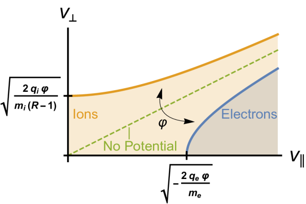
Figure 1: The passing region (shaded color) of midplane velocities $v_{\perp}$ and $v_{\parallel}$ for a magnetic mirror with mirror ratio $R$ and electrostatic potential drop $\varphi$. The passing region is given explicitly by Eq. 7, which can also be written as $v_{\perp}\leq\sqrt{(v_{\parallel}^{2}+2q_{s}\varphi/m_{s})/(R-1)}$; hence, the passing region generally takes the form depicted in the figure for $\varphi\geq 0$.

Let us consider a magnetic mirror field aligned along $\hat{x}$ in a two-dimensional ($2$-D) slab geometry with $\hat{z}$ an ignorable coordinate. Specifically, we take

$$\textbf{B}=B_{x}(x,y)\hat{x}+B_{y}(x,y)\hat{y}$$ (1)

such that

$$B_{x}(x,y)>0,\quad B_{y}(x,0)=0$$ (2a)

and for any $$x_{2}\geq x_{1}\geq 0$$,

$$|\textbf{B}(x_{2},y)|\geq|\textbf{B}(x_{1},y)|.$$ (2b)

We assume B to be sufficiently strong such that, neglecting collisions, the particle transport is dominated by dynamics along B. Let us also introduce a $1$-D electrostatic potential $\phi(x)$, which can either be externally imposed or be the ambipolar potential that arises from differential transport of electrons and ions. Finally, let us assume that the particle source is such that the distribution function is spatially confined near the mirror axis $y=0$ with a fixed velocity profile at $x=0$. Note that this initial condition implies that the particle dynamics are effectively $1$-D, with transverse drifts like the curvature drift and the $E\times B$ drift being negligible.

Suppose we are interested in the current associated with the passing particles at some plane $x=L$. For a single particle of species $s$ initialized on the mirror axis $y=0$, conservation of magnetic moment implies that Freidberg (2010)

$$\frac{v^{2}_{\perp,L}}{|\textbf{B}(L,0)|}=\frac{v^{2}_{\perp,0}}{|\textbf{B}(0,0)|},$$ (3)

while conservation of energy implies that

$$v^{2}_{\parallel,L}+v^{2}_{\perp,L}+\frac{2q_{s}}{m_{s}}\phi(L)=v^{2}_{\parallel,0}+v^{2}_{\perp,0}+\frac{2q_{s}}{m_{s}}\phi(0).$$ (4)

Here, $m_{s}$ and $q_{s}$ are respectively the mass and charge of species $s$, while $v_{\perp,x}$ and $v_{\parallel,x}$ denote respectively the perpendicular and parallel components of the particle velocity with respect to the magnetic field at position $x$.

Combining Eqs. 3 and 4 yields an expression for the exit velocity $v_{\parallel,L}$ in terms of the midplane velocities $v_{\parallel,0}$ and $v_{\perp,0}$ as

$$v_{\parallel,L}=\sqrt{v^{2}_{\parallel,0}-(R-1)v^{2}_{\perp,0}+\frac{2q_{s}}{m_{s}}\varphi},$$ (5)

where we have defined the mirror ratio and the potential drop along the mirror axis as respectively

$$R\doteq\frac{|\textbf{B}(L,0)|}{|\textbf{B}(0,0)|}\geq 1,\quad\varphi\doteq\phi(0)-\phi(L).$$ (6)

The ‘passing region’ is defined as the region of midplane velocities such that $v_{\parallel,L}$ is real, namely,

$$v^{2}_{\parallel,0}-(R-1)v^{2}_{\perp,0}+\frac{2q_{s}}{m_{s}}\varphi\geq 0.$$ (7)

As shown in Fig. 1, this is a region bounded by a hyperbolic curve which either intersects the $v_{\perp,0}$ axis ($q_{s}\varphi>0$), the $v_{\parallel,0}$ axis ($q_{s}\varphi<0$), or becomes a straight line intersecting the origin ($q_{s}\varphi=0$). See also Fig. 2 for a depiction of the passing region in midplane-energy space, rather than midplane-velocity space. Note that we require $x=L$ to be accessible, i.e., $v_{\parallel,x}\geq 0$ for all $0\leq x<L$ if $v_{\parallel,L}\geq 0$. This places constraints on the allowed spatial structure of $\phi(x)$.

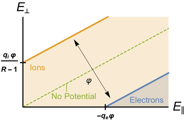
Figure 2: Same as Fig. 1 but for midplane energies $E_{\perp}=m_{s}v_{\perp}^{2}/2$ and $E_{\parallel}=m_{s}v_{\parallel}^{2}/2$. In these variables, the passing region (shaded) is simply $E_{\perp}\leq(E_{\parallel}+q_{s}\varphi)/(R-1)$.

Given the midplane velocity distribution $f_{s}(v_{\parallel,0},v_{\perp,0})$ for species $s$ (assumed to be gyrotropic for simplicity), the collected current of species $s$ at $x=L$ is obtained simply as the expectation value of Eq. 5:

$$\left\langle j_{s,L}\right\rangle =q_{s}\iint\limits_{\text{Passing}}\text{d}v_{\parallel,0}\,\text{d}v_{\perp,0}\,f_{s}\left(v_{\parallel,0},v_{\perp,0}\right)$$

$$\hskip 56.9055pt\times\sqrt{v^{2}_{\parallel,0}-(R-1)v^{2}_{\perp,0}+\frac{2q_{s}}{m_{s}}\varphi},$$ (8)

where the integration is taken over the passing region. When the distribution function is a Maxwellian with density $n_{s}$ and temperature $T_{s}$, given explicitly as

$$f_{s}\left(v_{\parallel,0},v_{\perp,0}\right) =n_{s}v_{\perp,0}\sqrt{\frac{m_{s}^{3}}{2\pi T_{s}^{3}}}$$

$$\hskip 11.38109pt\times\exp\left[-\frac{m_{s}}{2T_{s}}\left(v^{2}_{\parallel,0}+v^{2}_{\perp,0}\right)\right],$$ (9)

then Eq. 8 takes the form

$$\left\langle j_{s,L}\right\rangle=q_{s}n_{s}\sqrt{\frac{8T_{s}}{\pi m_{s}}}\mathcal{I}\left(\frac{q_{s}}{|q_{e}|}\frac{T_{e}}{T_{s}}\widetilde{\varphi};R\right),$$ (10)

where $\widetilde{\varphi}\doteq\frac{|q_{e}|\varphi}{T_{e}}$ is the potential drop normalized by the electron thermal energy and the (dimensionless) integral function $\mathcal{I}(X;R)$ is given as

$$\mathcal{I}(X;R) =\iint\limits_{\text{Passing}}\text{d}u\,\text{d}w\,w\sqrt{u^{2}-(R-1)w^{2}+X}$$

$$\hskip 62.59605pt\times\exp\left(-u^{2}-w^{2}\right).$$ (11)

In terms of the nondimensionalized velocities $u$ and $w$, the passing region is defined as the region such that

$$\text{Max}\left[0,\sqrt{(R-1)w^{2}-X}\right]\leq u<\infty,$$ (12a)

$$0\leq w\leq\sqrt{\frac{u^{2}+X}{R-1}}.$$ (12b)

Hence, $\mathcal{I}(X;R)$ can be written explicitly as

$$\mathcal{I}(X;R)=\left\{\begin{array}[]{lr}\int\limits_{0}^{\infty}\text{d}u\int\limits_{0}^{\sqrt{\frac{u^{2}+X}{R-1}}}\text{d}w\,w\sqrt{u^{2}-(R-1)w^{2}+X}\,\exp\left(-u^{2}-w^{2}\right)&X\geq 0\\[14.22636pt] \int\limits_{\sqrt{|X|}}^{\infty}\text{d}u\int\limits_{0}^{\sqrt{\frac{u^{2}-|X|}{R-1}}}\text{d}w~{}w\sqrt{u^{2}-(R-1)w^{2}-|X|}\,\exp\left(-u^{2}-w^{2}\right)&X<0\end{array}\right..$$ (13)

Then, as shown in Appendix A, $\mathcal{I}(X;R)$ can be simplified as

$$\mathcal{I}(X;R)=\left\{\begin{array}[]{lr}\frac{X}{8}\left[K_{1}\left(\frac{X}{2}\right)+K_{0}\left(\frac{X}{2}\right)\right]\exp\left(\frac{X}{2}\right)-\frac{\sqrt{X(R-1)}}{4}\,\mathcal{C}(X;R)\exp\left(\frac{X}{2}\right)&X>0\\[14.22636pt] \frac{1}{4}-\frac{R-1}{4\sqrt{R}}\,\operatorname{csch}^{-1}\left(\sqrt{R-1}\right)&X=0\\[14.22636pt] \frac{|X|}{8}\left[K_{1}\left(\frac{|X|}{2}\right)-K_{0}\left(\frac{|X|}{2}\right)\right]\exp\left(-\frac{|X|}{2}\right)-\frac{\sqrt{|X|(R-1)}}{4}\,\mathcal{S}(|X|;R)\exp\left(-\frac{|X|}{2}\right)&X<0\end{array}\right.,$$ (14)

where $K_{\nu}(X)$ is the modified Bessel function of the second kind Olver et al. (2010), and the auxiliary functions $\mathcal{C}$ and $\mathcal{S}$ are defined as

$$\mathcal{C}(X;R) =\int_{0}^{\infty}\text{d}t~{}\cosh\left(\frac{t}{2}\right)\mathcal{D}\left[\sqrt{\frac{X}{R-1}}\cosh\left(\frac{t}{2}\right)\right]\exp\left[-\frac{X}{2}\cosh(t)\right],$$ (15a)

$$\mathcal{S}(X;R) =\int_{0}^{\infty}\text{d}t~{}\sinh\left(\frac{t}{2}\right)\mathcal{D}\left[\sqrt{\frac{X}{R-1}}\sinh\left(\frac{t}{2}\right)\right]\exp\left[-\frac{X}{2}\cosh(t)\right],$$ (15b)

\begin{overpic}[width=433.62pt,trim=0.0pt 0.0pt 0.0pt 0.0pt,clip]{ISURF.pdf} \put(15.0,15.0){{\Large(a)}} \end{overpic}

\begin{overpic}[width=433.62pt,trim=0.0pt 0.0pt 0.0pt 0.0pt,clip]{phiSURF.pdf} \put(15.0,15.0){{\Large(b)}} \end{overpic}

Figure 3: (a) The integral function $\mathcal{I}(X;R)$, given explicitly in Eq. 14. (b) Ambipolar potential $\widetilde{\varphi}$ obtained from solving Eq. 16 over the depicted range of temperature ratio and mirror ratio $R$.

with $\mathcal{D}(z)$ being the Dawson function Olver et al. (2010); Press et al. (2007). In this form, $\mathcal{I}(X;R)$ can be tabulated for discrete values of $X$ and $R$ using standard quadrature and special functions packages for subsequent interpolations. Figure 3(a) shows $\mathcal{I}(X;R)$ for $X\in[-5,10]$ and $R\in[1,5]$.

Often, the potential drop $\widetilde{\varphi}$ is the ambipolar potential that ensures no net current is collected at the mirror exit $x=L$. For a two-component plasma, this means $\left\langle j_{i,L}\right\rangle+\left\langle j_{e,L}\right\rangle=0$, or equivalently for specific case of Maxwellian midplane distributions,

$$\sqrt{\frac{m_{e}}{m_{i}}\frac{T_{i}}{T_{e}}}\mathcal{I}\left(\frac{q_{i}}{|q_{e}|}\frac{T_{e}}{T_{i}}\widetilde{\varphi};R\right)-\mathcal{I}(-\widetilde{\varphi};R)=0,$$ (16)

after using the quasineutrality condition $q_{i}n_{i}=|q_{e}|n_{e}$. The resultant ambipolar potential $\widetilde{\varphi}$ can thus be obtained from Eq. 16 via standard root-finding methods. Figure 3(b) shows the ambipolar $\widetilde{\varphi}$ for Hydrogen plasma for $T_{i}/T_{e}\in[0.2,2]$ and $R\in[1,5]$.

The dependencies of the ambipolar potential on the mirror ratio as well as ion temperature can be physically understood as follows. When $R=1$, i.e., when there is no magnetic mirror, the ambipolar potential decreases with increasing ion temperature, since the difference between the ion and electron thermal speed decreases with increasing ion temperature. This trend reverses for $R>1$, however, where increasing the ion temperature increases the ambipolar potential. This seemingly counter-intuitive result arises because the passing ion fraction $\eta_{i}$ decreases exponentially with increasing ion temperature, as shown in Fig. 4. Details of the passing fraction calculation are included in Appendix B. Hence, the (now fewer) passing ions must be accelerated to higher velocities by a larger potential in order to balance the passing electron current. Lastly, at fixed ion and electron temperature, we observe that the ambipolar potential decreases with increasing $R$. This is simply because more electrons are trapped by the mirror field, resulting in a smaller electron passing current.

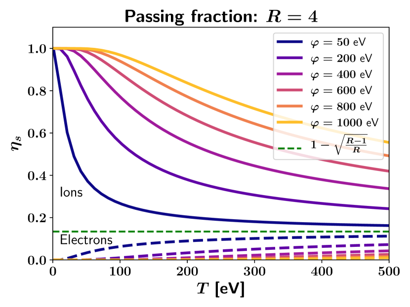
Figure 4: Passing particle fraction $\eta_{s}$ for ions (solid lines) and electrons (dashed lines) in a magnetic mirror with $R=4$ and various potential drops as the temperature is varied. The ion passing fraction is calculated with Eq. 35, while the electron passing fraction is calculated with Eq. 37.

Notably, the exponential dependence of the ion passing fraction on temperature has important consequences for ion confinement estimates. Although the particle passing fraction asymptotically approaches the oft-quoted neoclassical limit as $T/\varphi\to\infty$ (shown by the green dashed line in Fig. 4), this high temperature limit is rarely met in reality because $\varphi$ is typically comparable to $T_{e}$, being set by the ambipolar condition (Eq. 16 in our case) Stangeby (2000). Hence, the differences in estimated trapped particle fractions when using the neoclassical estimate versus the results of Fig. 4 can be significant.

For example, the LTX SOL plasma typically has $T_{e}=200$ eV, $T_{i}=40$ eV, $R=4$, and $\varphi=0.5\sim 3T_{e}=100\sim 600$ eV; we therefore estimate ion passing fraction as $\eta_{i}\gtrsim 0.8$. This is in drastic contradiction to the trapped fraction of $0.8-0.9$ (i.e., $\eta_{i}\lesssim 0.2$) from the neoclassical estimate which uses only the mirror ratio Majeski et al. (2017). This trend also holds for a more general SOL plasma with $T_{i}\approx T_{e}$ and low collisionality - $\eta_{i}$ will be moderately lower than the above LTX-based estimate, but is still expected to be significantly higher than the neoclassical estimate due to the presence of $\varphi$. Hence, we conclude that despite the relatively high mirror ratio of the ST magnetic geometry, the ions in a collisionless SOL are still not mirror-confined, and their main loss mechanism remains direct streaming to the limiters.

III Benchmarking the SOLFI full orbit particle code

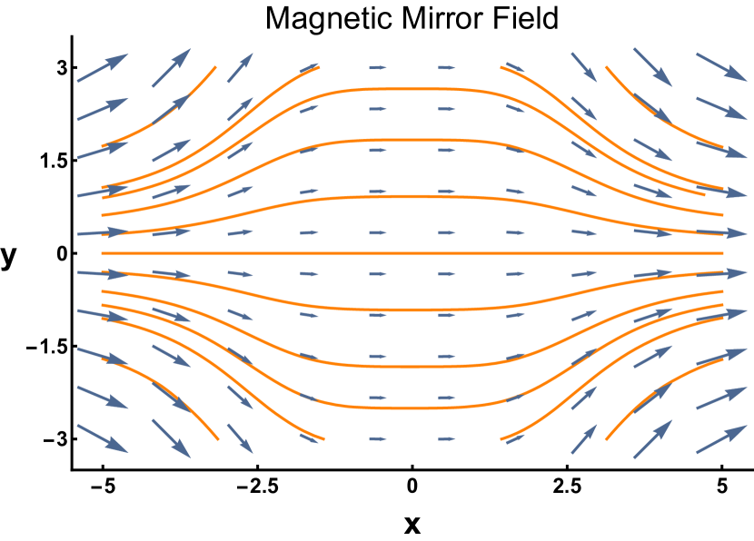
Figure 5: Magnetic mirror geometry used in the presented code benchmarking. The magnetic field lines obtained as the level sets of the stream function $\psi(x,y)$ [Eq. 17] are shown in orange, while the strength and orientation of the resulting magnetic field [Eqs. 18] is depicted by the blue arrows. For this particular case, $R=4$, $\ell=3$, and $B_{0}=3$.

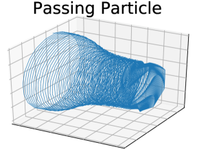
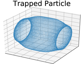
Figure 6: Sample orbits for passing (left) and trapped (right) particles in a magnetic mirror with no imposed electrostatic potential. Particle orbits are traced up to 1 million time steps or until particle hits the edge of computational domain. The first 5,000 steps are shown for the trapped particle.

SOLFI is a full-orbit Monte-Carlo particle tracer code that aims to simulate the fast ion orbits that traverse both the core and the SOL plasma in a tokamak. It is under development as a possible extension to the NBI code NUBEAM Pankin et al. (2004) to include SOL effects and aid better understanding of the influence of the SOL on fast particle confinement. That said, the particle tracer code itself is flexible in terms of magnetic geometry (Cartesian or toroidal) and is capable of simulating the dynamics of non-relativistic charged particles of arbitrary species in a variety of magnetic and electric field configurations. Here we benchmark the numerical methods of the code with the test case of particle losses in a collisionless magnetic mirror. (A more complete description of the SOLFI code will be reported elsewhere.)

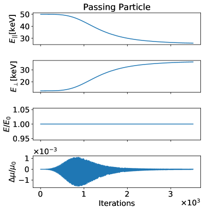
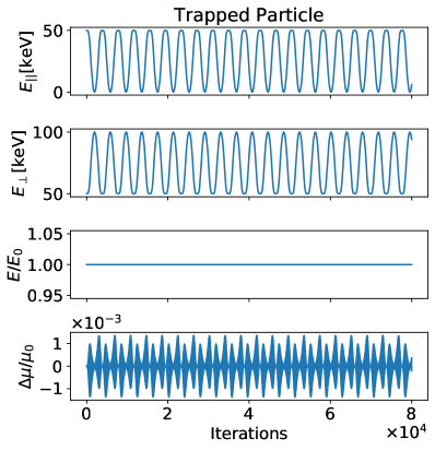
Figure 7: Example time evolution of energy and magnetic moment of a passing particle (left) and trapped particle (right) moving in the magnetic mirror field of Eq. 18 without an imposed electric potential, with energies typical for NBI ions in NSTX-U. The parallel, perpendicular, and total energy as well as the change in the magnetic moment of the particles are shown. The first 20 bounces are shown for the trapped particle. Energy is perfectly conserved as expected, while magnetic moment oscillates around a constant value. Simulations for other energies are qualitatively similar.

III.1 Magnetic field and electric potential profiles of a simple magnetic mirror

To perform the benchmarking, we require an analytical magnetic mirror field in 2-D slab geometry. Recall that if $\textbf{B}(x,y)$ is a two-component divergence-free vector field, then it can be described by a scalar stream function $\psi(x,y)$ such that $B_{x}(x,y)=\partial\psi/\partial y$ and $B_{y}(x,y)=-\partial\psi/\partial x$. As such, the level sets of $\psi(x,y)$ trace out the field lines of $\textbf{B}(x,y)$. For an ideal magnetic mirror, a possible stream function is given by the 2-parameter family

$$\psi(x,y;R,\ell)=B_{0}\,y\left[\frac{R-1}{\left(x/\ell\right)^{4}+1}+1\right]^{-1}.$$ (17)

The magnetic field components are therefore given as

$$B_{x}(x,y;R,\ell) =B_{0}\frac{1+\left(x/\ell\right)^{4}}{R+\left(x/\ell\right)^{4}},$$ (18a)

$$B_{y}(x,y;R,\ell) =-B_{0}\,(R-1)\frac{4\left(x/\ell\right)^{3}\left(y/\ell\right)}{\left[R+\left(x/\ell\right)^{4}\right]^{2}},$$ (18b)

where $R$ is the mirror ratio and $\ell$ roughly describes the width of the magnetic well. Notably, along the mirror axis ($y=0$) the ratio of the magnetic field intensities at midplane and at the mirror end is precisely given by $R$, i.e., $|\textbf{B}(\pm\infty,0;R,\ell)|/|\textbf{B}(0,0;R,\ell)|=R$. Sample field lines are shown in figure 5.

As for the imposed electric potential, it is sufficient for our purposes to choose the spatial profile

$$\phi(x)=\phi_{m}\cos^{6}\left(\pi x/6\ell\right),$$ (19)

where $\phi_{m}$ is potential at midplane $x=0$, and the length scale $\ell$ in Eq. 19 is the same $\ell$ that occurs in the magnetic field profile in Eq. 18. This specific functional form of $\phi$ is chosen to ensure that the collection plane $x=\pm 3\ell$ in our benchmarking study is accessible to all initialized particles (see Sec. II), although we note that it is not necessarily the self-consistent potential field that would result from the particle motion.

The simulation domain is chosen as $x\in[-3\ell,3\ell]$ and $y,z\in[-10\ell,10\ell]$, where the magnetic axis is along the $\hat{x}$ direction. The large size of domain in the perpendicular direction is chosen to allow the perpendicular scale length of the magnetic field to be much larger than the particle Larmor radius, such that all curvature and gradient drifts are negligible and cross field losses do not occur. The choice to have the collection plane at $x=\pm 3\ell$ is simply because $|\textbf{B}(3\ell,0;R,\ell)/\textbf{B}(0,0;R,\ell)|$ is satisfactorily close to the (desired) asymptotic mirror ratio $R$.

III.2 Charged particle dynamics

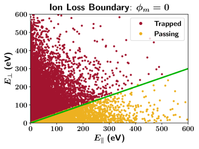
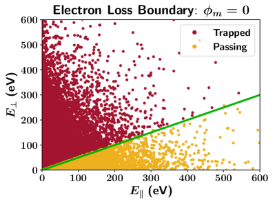
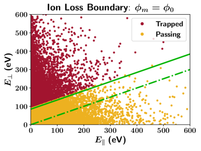
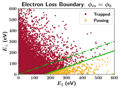
Figure 8: Ion and electron passing boundaries from full-orbit simulations. Particles are initialized according to the Maxwellian distribution of Eq. 9 with LTX-like thermal plasma parameters $T_{i}=T_{e}=100$ eV. Mirror ratio in this simulation is set to be $R=3$. Each point represents the initial energy-space location of a particle. Ten thousand particles are injected at the midplane and followed for up to 1 million time steps. Dashed green lines are the expected passing boundary in absence of electric potential, whereas solid green lines are the expected loss boundaries with ambipolar potential $\phi_{0}$ imposed, where $\phi_{0}$ satisfies Eq. 16. The simulated passing boundaries show excellent agreement with predictions. Number of particles is $N=20,000$. Note that simulations performed with NSTX-like thermal plasma parameters $T_{i}=T_{e}\approx 1000$ eV are qualitatively similar and therefore not presented.

The equations of motion for charged particles is simply the combination of Coulomb and Lorentz force:

$$\frac{\text{d}\textbf{x}}{\text{d}t} =\textbf{v},$$ (20a)

$$m_{s}\frac{\text{d}\textbf{v}}{\text{d}t} =-q_{s}\frac{\text{d}\phi(x)}{\text{d}x}\hat{x}+q_{s}\textbf{v}\times\textbf{B},$$ (20b)

where the electrostatic potential is assumed to vary only in the $\hat{x}$ direction. The equations of motion is numerically integrated with the Boris algorithm Boris (1970), which guarantees energy conservation Qin et al. (2013). Examples of passing and trapped particle orbits in the mirror field of Eq. 18 without an electrostatic potential drop are shown in Fig. 6. Figure 7 shows the corresponding time evolution of parallel, perpendicular, and total energy as well as the magnetic moments of the passing and trapped particles with energies similar to those of NBI ions in NSTX-U. It can be seen that while the parallel and perpendicular energies transfer back and forth between bounces, the total energy of the particles are conserved exactly. The magnetic moment is calculated as $E_{\perp}/B$, which exhibits small oscillations around a constant value. This small oscillation has been previously explained as the truncation error of the full adiabatic expansion Belova et al. (2003), which is an artifact of the simple $\mu=E_{\perp}/B$ representation and not cause for concern since the oscillation is also bounded.

To verify the passing/trapped boundary of sample particles, a collection of 20,000 particles are launched into the magnetic midplane $x=0$ with Maxwellian velocity distribution. The particles are pushed up to 1 million timesteps, with $\sim 5$ steps per Larmor period. Particles that reach the mirror end at $x=\pm 3\ell$ are flagged as “passing”, or “trapped” otherwise. Figure 8 shows the initial energy space distribution of the test particles and whether they are trapped or lost, with and without the ambipolar potential that satisfies Eq. 16. The simulated passing boundaries show excellent agreement with theoretical predictions. (Simulations were performed for a range of thermal plasma parameters, and the results are all qualitatively similar to those presented in Fig. 8.)

We shall now verify that the net passing current indeed vanishes for the ambipolar potential drop $\varphi$ that satisfies Eq. 16. To calculate the passing current, the parallel velocities of the particles when they reach the mirror end are recorded and then summed. This sum of velocities is proportional to the total passing particle current. Both electron and ion current are calculated as a function of the midplane potential with fixed electron temperature, but varying ion temperature and mirror ratio $R$. The resulting current is shown in Fig. 9, where the ion and electron currents are seen to converge as the midplane potential approaches the predicted ambipolar value $\phi_{0}$ in all cases.

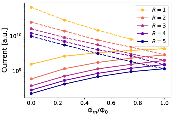
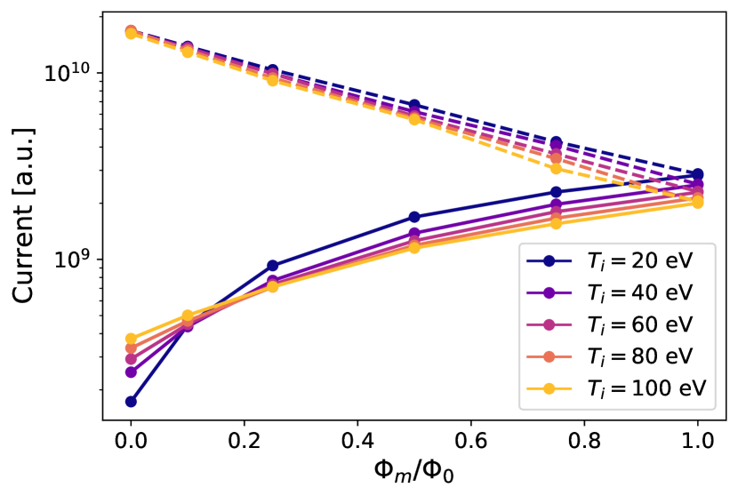
Figure 9: Convergence of electron (dashed lines) and ion (solid lines) passing current as the midplane potential $\phi_{m}$ approaches the theoretical value $\phi_{0}$ for the ambipolar potential that satisfies Eq. 16. (top) Mirror ratio $R$ is varied and $T_{i}=T_{e}$. (bottom) $T_{i}$ is varied, $T_{e}=100$ eV and $R=3$. The passing current is calculated as the sum of particle velocities for the passing particles as they escape the magnetic mirror. Note that $20,000$ particles are used to obtain each data point.

IV Conclusion

In this paper we present the benchmarking results of the full-orbit Monte Carlo particle code SOLFI in a simple magnetic mirror. The passing particle current and the resulting ambipolar potential are derived analytically and compared to the simulation results, which show excellent agreement. The conservation properties of energy and magnetic moment of the particle tracing algorithm is demonstrated, and example 3D particle orbits are presented. The simulated passing/trapped boundary with and without the ambipolar potential also show excellent agreement with predictions. Overall, the collisionless particle tracing algorithm of SOLFI is consistent with expectations.

The passing particle fraction $\eta_{s}$ and associated current density $j_{s}$ in the presence of a electrostatic potential drop $\varphi$ is also derived. For particle species with relatively low temperatures ($T/\varphi$ not too large), the passing fraction is exponentially modified by $\varphi$. In particular, the thermal SOL ions in STs such as LTX remain untrapped by magnetic mirror field even when collisions are neglected. The exponential dependence of $\eta_{s}$ on $\varphi$ suggests that even in the closed field line regions of tokamak plasmas, a strong electric field may have a significant effect on neoclassical particle confinement.

For example, strong radial electric fields are known to exist in the H-mode pedestal as a result of the pressure gradient Wang et al. (2001). The electrostatic potential drop associated with this radial electric field across a trapped ion banana orbit is typically on the order of $T_{i}$ Kagan and Catto (2010). Our results suggest that this electrostatic potential drop could have strong consequences for neoclassical processes where trapped particles play a significant role, such as the bootstrap current Kagan and Catto (2010); Watanabe et al. (1995). These effects along with fast ion transport in tokamak edge plasmas will be the subject of further studies. Numerical algorithms for collisions of the tracer particles with a thermal plasma background are being developed in parallel Zhang et al. (2020); Fu et al. (2020) and will be included in future versions of SOLFI, which will allow for more realistic predictions and aid physics understandings.

Data Availability

The data that support the findings of this study are available from the corresponding author upon reasonable request.

Appendix A Derivation of Eq. 14

Here we derive Eq. 14 from Eq. 13. Let us first consider the inner integration over $w$, which has the general form

$$\int_{0}^{\sqrt{a}}\text{d}w\,w\sqrt{a-w^{2}}~{}e^{-w^{2}}=e^{-a}\int_{0}^{\sqrt{a}}\text{d}t\,t^{2}e^{t^{2}},$$ (21)

where we transformed the integration variable from $w$ to $t\doteq\sqrt{a-w^{2}}$. Note that $a=(u^{2}+X)/(R-1)$ in terms of Eq. 13. Integration by parts then yields

$$e^{-a}\int_{0}^{\sqrt{a}}\text{d}t\,t^{2}e^{t^{2}} =\left.\frac{t}{2}e^{t^{2}-a}\right|_{0}^{\sqrt{a}}-\frac{1}{2}e^{-a}\int_{0}^{\sqrt{a}}\text{d}t~{}e^{t^{2}}$$

$$=\frac{\sqrt{a}}{2}-\frac{1}{2}\mathcal{D}(\sqrt{a}),$$ (22)

where $\mathcal{D}(z)$ is the Dawson function Olver et al. (2010); Press et al. (2007), defined as

$$\mathcal{D}(z)=e^{-z^{2}}\int_{0}^{z}\text{d}t~{}e^{t^{2}}.$$ (23)

Let us first consider the case when $X>0$. Substituting Eq. 22 into Eq. 13 yields

$$\mathcal{I}(X>0;R) =\int\limits_{0}^{\infty}\text{d}u\,\frac{\sqrt{u^{2}+X}}{2}\,e^{-u^{2}}$$

$$-\frac{\sqrt{R-1}}{2}\int\limits_{0}^{\infty}\text{d}u\,\mathcal{D}\left(\sqrt{\frac{u^{2}+X}{R-1}}\right)e^{-u^{2}}.$$ (24)

The variable transformation $u=\sqrt{X}\sinh(t/2)$ then yields

$$\mathcal{I}(X>0;R) =\int_{0}^{\infty}\text{d}t\,\frac{X\left[\cosh(t)+1\right]}{8}\exp\left[\frac{X}{2}-\frac{X}{2}\cosh\left(t\right)\right]$$

$$\hskip 11.38109pt-\frac{\sqrt{X(R-1)}}{4}\,\mathcal{C}(X;R)\exp\left(\frac{X}{2}\right),$$ (25)

where $\mathcal{C}(X;R)$ is defined in Eq. 15a. By recognizing the Sommerfeld integral representation Olver et al. (2010); Watson (1966):

$$K_{\nu}(z)=\int_{0}^{\infty}\text{d}t~{}\cosh\left(\nu t\right)\exp\left[-z\cosh(t)\right],$$ (26)

then Eq. 25 can be simplified to the top line of Eq. 14.

Let us next consider the case when $X<0$ and Eq. 13 takes the form

$$\mathcal{I}(X<0;R) =\int\limits_{\sqrt{|X|}}^{\infty}\text{d}u\,\frac{\sqrt{u^{2}-|X|}}{2}e^{-u^{2}}$$

$$-\frac{\sqrt{R-1}}{2}\int\limits_{\sqrt{|X|}}^{\infty}\text{d}u\,\mathcal{D}\left(\sqrt{\frac{u^{2}-|X|}{R-1}}\right)e^{-u^{2}}.$$ (27)

The variable transformation $u=\sqrt{|X|}\cosh(t/2)$ then yields

$$\mathcal{I}(X<0;R) =\int_{0}^{\infty}\text{d}t\,\frac{X\left[1-\cosh(t)\right]}{8}\exp\left[\frac{X}{2}+\frac{X}{2}\cosh\left(t\right)\right]$$

$$\hskip 11.38109pt-\frac{\sqrt{X(1-R)}}{4}\,\mathcal{S}(|X|;R)\exp\left(\frac{X}{2}\right),$$ (28)

where $\mathcal{S}(X;R)$ is defined in Eq. 15b. As before, invoking Eq. 26 simplifies Eq. 28 to the bottom line of Eq. 14.

Finally, let us consider $X=0$. After noting that

$$\int_{0}^{\infty}\text{d}u\,u\,e^{-u^{2}}=\frac{1}{2},$$ (29)

substitution of Eq. 22 into Eq. 13 yields

$$\mathcal{I}(0;R) =\frac{1}{4}-\frac{\sqrt{R-1}}{2}\int\limits_{0}^{\infty}\text{d}u\,\mathcal{D}\left(\frac{u}{\sqrt{R-1}}\right)e^{-u^{2}}.$$ (30)

By making use of the identity Oldham et al. (2009)

$$\int_{0}^{\infty}\text{d}u\,\mathcal{D}(au)e^{-bu^{2}}=\frac{\operatorname{csch}^{-1}\left(\frac{\sqrt{b}}{a}\right)}{2\sqrt{a^{2}+b}},\quad a,\,b>0,$$ (31)

one simplifies Eq. 30 to the middle line of Eq. 14.

Appendix B Passing particle fraction

Here, we derive the passing particle fraction in an ideal mirror with potential drop $\varphi$ for the gyrotropic Maxwellian distribution function provided in Eq. 9. By definition, the fraction of passing particles for species $s$ with respect to all particles with $v_{\parallel,0}\geq 0$, denoted $\eta_{s}$, is given when $q_{s}\varphi\geq 0$ as

$$\eta_{s}=\frac{4}{\sqrt{\pi}}\int_{0}^{\infty}\text{d}u\,e^{-u^{2}}\int_{0}^{\sqrt{a}}\text{d}w\,we^{-w^{2}},$$ (32)

or when $q_{s}\varphi<0$ as

$$\eta_{s}=\frac{4}{\sqrt{\pi}}\int_{\sqrt{\frac{|q_{s}\varphi|}{T_{s}}}}^{\infty}\text{d}u\,e^{-u^{2}}\int_{0}^{\sqrt{a}}\text{d}w\,we^{-w^{2}},$$ (33)

where we have introduced $a\doteq(u^{2}+q_{s}\varphi/T_{s})/(R-1)$. We readily evaluate

$$\int_{0}^{\sqrt{a}}\text{d}w\,w\,e^{-w^{2}}=\frac{1}{2}-\frac{1}{2}e^{-a}.$$ (34)

Hence, for $q_{s}\varphi\geq 0$ we obtain

$$\eta_{s} =\frac{2}{\sqrt{\pi}}\left\{1-\sqrt{\frac{R-1}{R}}\exp\left[-\frac{q_{s}\varphi_{s}}{T_{s}(R-1)}\right]\right\}$$

$$\hskip 11.38109pt\times\int_{0}^{\infty}\text{d}u\,\exp\left(-u^{2}\right)$$

$$=1-\sqrt{\frac{R-1}{R}}\exp\left[-\frac{q_{s}\varphi_{s}}{T_{s}(R-1)}\right].$$ (35)

Note that when $\varphi=0$, $\eta_{s}$ becomes independent of the species temperature $T_{s}$.

By making use of the identity

$$\int_{a}^{\infty}\text{d}x\,e^{-bx^{2}}=\frac{1}{2}\sqrt{\frac{\pi}{a}}\,\operatorname{erfc}\left(a\sqrt{b}\right),\quad a,\,b>0,$$ (36)

one can show that for $q_{s}\varphi<0$, $\eta_{s}$ takes the form

$$\eta_{s} =\text{erfc}\left(\sqrt{\frac{|q_{s}\varphi|}{T_{s}}}\right)$$

$$-\sqrt{\frac{R-1}{R}}\operatorname{erfc}\left(\sqrt{\frac{|q_{s}\varphi|}{T_{s}}\frac{R}{R-1}}\right)\exp\left[\frac{|q_{s}\varphi|}{T_{s}(R-1)}\right].$$ (37)

Representative traces of Eq. 35 and Eq. 37 are shown in Fig. 4 of the main text. Clearly, the fraction of passing ions $\eta_{i}$ decreases exponentially with increasing temperature. In fact, the passing fraction of both species approach the asymptotic value $1-\sqrt{(R-1)/R}$ as the temperature is increased.

References

- Peng and Strickler (1986) Y.-K. M. Peng and D. J. Strickler, Nucl. Fusion 26, 769 (1986).
- Peng (2000) Y.-K. M. Peng, Phys. Plasmas 7, 1681 (2000).
- Ono and Kaita (2015) M. Ono and R. Kaita, Phys. Plasmas 22, 040401 (2015).
- Kaye et al. (2019) S. M. Kaye, D. J. Battaglia, D. Baver, E. Belova, J. W. Berkery, V. N. Duarte, N. Ferraro, E. Fredrickson, N. Gorelenkov, W. Guttenfelder, and G. Z. Hao, Nucl. Fusion 59, 112007 (2019).
- Eriksson and Porcelli (2001) L. G. Eriksson and F. Porcelli, Plasma Phys. Control. Fusion 43, R145 (2001).
- Heidbrink and Sadler (1994) W. W. Heidbrink and G. J. Sadler, Nucl. Fusion 34, 535 (1994).
- Thomas et al. (1998) P. R. Thomas, P. Andrew, B. Balet, D. Bartlett, J. Bull, B. De Esch, A. Gibson, C. Gowers, H. Guo, G. Huysmans, and T. Jones, Phys. Rev. Lett. 80, 5548 (1998).
- Budny et al. (2016) R. V. Budny, J. G. Cordey, TFTR Team, and JET Contributors, Nucl. Fusion 56, 056002 (2016).
- Hao et al. (2018) G. Z. Hao, W. W. Heidbrink, D. Liu, M. Podesta, L. Stagner, R. E. Bell, A. Bortolon, and F. Scotti, Plasma Phys. Control. Fusion 60, 025026 (2018).
- Liu et al. (2018) D. Liu, W. W. Heidbrink, M. Podestà, G. Z. Hao, D. S. Darrow, E. D. Fredrickson, and D. Kim, Nucl. Fusion 58, 082028 (2018).
- Buangam et al. (2020) W. Buangam, J. Garcia, T. Onjun, and JET Contributors, Plasma Sci. Technol. 22, 065101 (2020).
- Lestz et al. (2021) J. Lestz, E. Belova, and N. N. Gorelenkov, Nucl. Fusion (2021).
- Belova et al. (2003) E. V. Belova, N. N. Gorelenkov, and C. Z. Cheng, Phys. Plasmas 10, 3240 (2003).
- Belova et al. (2019) E. V. Belova, E. D. Fredrickson, J. B. Lestz, N. A. Crocker, and NSTX-U Team, Phys. Plasmas 26, 092507 (2019).
- Van Zeeland et al. (2019) M. A. Van Zeeland, C. S. Collins, W. W. Heidbrink, M. E. Austin, X. D. Du, V. N. Duarte, A. Hyatt, G. Kramer, N. Gorelenkov, B. Grierson, and D. Lin, Nucl. Fusion 59, 086028 (2019).
- Van Zeeland et al. (2021) M. A. Van Zeeland, L. Bardoczi, J. G. Martin, W. W. Heidbrink, M. Podesta, M. E. Austin, C. Collins, X. Du, V. N. Duarte, M. Garcia-Munoz, and S. Munaretto, Nucl. Fusion 61, 066028 (2021).
- Yang et al. (2021) J. Yang, M. Podestà, and E. D. Fredrickson, Plasma Phys. Control. Fusion 63, 045003 (2021).
- Kim et al. (2019) D. Kim, M. Podesta, D. Liu, G. Hao, and F. M. Poli, Nucl. Fusion 59, 086007 (2019).
- Podesta et al. (2019) M. Podesta, L. Bardoczi, C. Collins, N. N. Gorelenkov, W. W. Heidbrink, V. N. Duarte, G. J. Kramer, E. D. Fredrickson, M. Gorelenkova, D. Kim, and D. Liu, Nucl. Fusion 59, 106013 (2019).
- McClements and Fredrickson (2017) K. G. McClements and E. D. Fredrickson, Plasma Phys. Control. Fusion 59, 053001 (2017).
- Jaworski et al. (2013) M. A. Jaworski, T. Abrams, J. P. Allain, M. G. Bell, R. E. Bell, A. Diallo, T. K. Gray, S. P. Gerhardt, R. Kaita, H. W. Kugel, and B. P. LeBlanc, Nucl. Fusion 53, 083032 (2013).
- Evtikhin et al. (2002) V. A. Evtikhin, I. E. Lyublinski, A. V. Vertkov, S. V. Mirnov, V. B. Lazarev, N. P. Petrova, S. M. Sotnikov, A. P. Chernobai, B. I. Khripunov, V. B. Petrov, and D. Y. Prokhorov, Plasma Phys. Control. Fusion 44, 955 (2002).
- Nagayama (2009) Y. Nagayama, Fusion Eng. Des. 84, 1380 (2009).
- Rognlien et al. (2019) T. D. Rognlien, M. E. Rensink, E. Emdee, R. J. Goldston, J. Schwartz, and D. Stotler, Nucl. Mater. Energy 18, 233 (2019).
- Poradziński et al. (2019) M. Poradziński, I. Ivanova-Stanik, G. Pełka, V. P. Ridolfini, and R. Zagórski, Fusion Eng. Des. 146, 1500 (2019).
- Ono and Raman (2020) M. Ono and R. Raman, J. Fusion Energy , 1 (2020).
- Emdee et al. (2019) E. D. Emdee, R. J. Goldston, J. A. Schwartz, M. Rensink, and T. D. Rognlien, Nucl. Fusion 59, 086043 (2019).
- Majeski et al. (2010) R. Majeski, H. Kugel, R. Kaita, S. Avasarala, M. G. Bell, R. E. Bell, L. Berzak, P. Beiersdorfer, S. P. Gerhardt, E. Granstedt, T. Gray, C. Jacobson, J. Kallman, S. Kaye, T. Kozub, B. P. LeBlanc, J. Lepson, D. P. Lundberg, R. Maingi, D. Mansfield, S. F. Paul, G. V. Pereverzev, H. Schneider, V. Soukhanovskii, T. Strickler, D. Stotler, J. Timberlake, L. E. Zakharov, and The NSTX and LTX Research Teams, Fusion Eng. Des. 85, 1283 (2010).
- Mansfield et al. (2001) D. K. Mansfield, D. W. Johnson, B. Grek, H. W. Kugel, M. G. Bell, R. E. Bell, R. V. Budny, C. E. Bush, E. D. Fredrickson, K. W. Hill, and D. L. Jassby, Nucl. Fusion 41, 1823 (2001).
- Mirnov et al. (2003) S. V. Mirnov, V. B. Lazarev, S. M. Sotnikov, T-11M Team, V. A. Evtikhin, I. E. Lyublinski, and A. V. Vertkov, Fusion Eng. Des. 65, 455 (2003).
- Apicella et al. (2007) M. L. Apicella, G. Mazzitelli, V. P. Ridolfini, V. Lazarev, A. Alekseyev, A. Vertkov, R. Zagorski, and FTU Team, J. Nucl. Mater. 363, 1346 (2007).
- Kugel et al. (2008) H. W. Kugel, M. G. Bell, J.-W. Ahn, J. P. Allain, R. Bell, J. Boedo, C. Bush, D. Gates, T. Gray, S. Kaye, and R. Kaita, Phys. Plasmas 15, 056118 (2008).
- Majeski et al. (2017) R. Majeski, R. E. Bell, D. P. Boyle, R. Kaita, T. Kozub, B. P. LeBlanc, M. Lucia, R. Maingi, E. Merino, Y. Raitses, J. C. Schmitt, J. P. Allain, F. Bedoya, J. Bialek, T. M. Biewer, J. M. Canik, L. Buzi, B. E. Koel, M. I. Patino, A. M. Capece, C. Hansen, T. Jarboe, S. Kubota, W. A. Peebles, and K. Tritz, Phys. Plasmas 24, 056110 (2017).
- Boyle et al. (2017) D. P. Boyle, R. Majeski, J. C. Schmitt, C. Hansen, R. Kaita, S. Kubota, M. Lucia, and T. D. Rognlien, Phys. Rev. Lett. 119, 015001 (2017).
- Zakharov et al. (2004) L. E. Zakharov, N. N. Gorelenkov, R. B. White, S. I. Krasheninnikov, and G. V. Pereverzev, Fusion Eng. Des. 72, 149 (2004).
- Krasheninnikov et al. (2003) S. I. Krasheninnikov, L. E. Zakharov, and G. V. Pereverzev, Phys. Plasmas 10, 1678 (2003).
- Zhang et al. (2019) X. Zhang, D. B. Elliott, A. Maan, D. P. Boyle, R. Kaita, and R. Majeski, Nucl. Mater. Energy 19, 250 (2019).
- Emdee et al. (2021) E. D. Emdee, R. J. Goldston, J. D. Lore, and X. Zhang, Nucl. Mater. Energy 27, 101004 (2021).
- Stangeby (2000) P. C. Stangeby, The plasma boundary of magnetic fusion devices, Vol. 224 (New York: Taylor and Francis, 2000).
- Goldston (2011) R. J. Goldston, Nucl. Fusion 52, 013009 (2011).
- Pankin et al. (2004) A. Pankin, D. McCune, R. Andre, G. Bateman, and A. Kritz, Comput. Phys. Commun. 159, 157 (2004).
- Majeski et al. (2009) R. Majeski, L. Berzak, T. Gray, R. Kaita, T. Kozub, F. Levinton, D. P. Lundberg, J. Manickam, G. V. Pereverzev, K. Snieckus, V. Soukhanovskii, J. Spaleta, D. Stotler, T. Strickler, J. Timberlake, J. Yoo, and L. Zakharov, Nucl. Fusion 49, 055014 (2009).
- Menard et al. (2012) J. E. Menard, S. Gerhardt, M. Bell, J. Bialek, A. Brooks, J. Canik, J. Chrzanowski, M. Denault, L. Dudek, D. A. Gates, N. Gorelenkov, W. Guttenfelder, R. Hatcher, J. Hosea, R. Kaita, S. Kaye, C. Kessel, E. Kolemen, H. Kugel, R. Maingi, M. Mardenfeld, D. Mueller, B. Nelson, C. Neumeyer, M. Ono, E. Perry, R. Ramakrishnan, R. Raman, Y. Ren, S. Sabbagh, M. Smith, V. Soukhanovskii, T. Stevenson, R. Strykowsky, D. Stutman, G. Taylor, P. Titus, K. Tresemer, K. Tritz, M. Viola, M. Williams, R. Woolley, H. Yuh, H. Zhang, Y. Zhai, A. Zolfaghari, and the NSTX Team, Nucl. Fusion 52, 083015 (2012).
- Freidberg (2010) J. P. Freidberg, Plasma Physics and Fusion Energy (Cambridge: Cambridge University Press, 2010).
- Olver et al. (2010) F. W. J. Olver, D. W. Lozier, R. F. Boisvert, and C. W. Clark, NIST Handbook of Mathematical Functions (Cambridge: Cambridge University Press, 2010).
- Press et al. (2007) W. H. Press, S. A. Teukolsky, W. T. Vetterling, and B. P. Flannery, Numerical Recipes, 3rd ed. (Cambridge: Cambridge University Press, 2007).
- Boris (1970) J. P. Boris, in Proc. Fourth Conf. Num. Sim. Plasmas (1970) pp. 3–67.
- Qin et al. (2013) H. Qin, S. Zhang, J. Xiao, J. Liu, Y. Sun, and W. M. Tang, Phys. Plasmas 20, 084503 (2013).
- Wang et al. (2001) W. X. Wang, F. L. Hinton, and S. K. Wong, Phys. Rev. Lett. 87, 055002 (2001).
- Kagan and Catto (2010) G. Kagan and P. J. Catto, Phys. Rev. Lett. 105, 045002 (2010).
- Watanabe et al. (1995) K. Y. Watanabe, N. Nakajima, M. Okamoto, K. Yamazaki, Y. Nakamura, and M. Wakatani, Nucl. Fusion 35, 335 (1995).
- Zhang et al. (2020) X. Zhang, Y. Fu, and H. Qin, Phys. Rev. E 102, 033302 (2020).
- Fu et al. (2020) Y. Fu, X. Zhang, and H. Qin, arXiv preprint arXiv:2010.12920 (2020).
- Watson (1966) G. N. Watson, A Treatise on the Theory of Bessel Functions, 2nd ed. (Cambridge: Cambridge University Press, 1966).
- Oldham et al. (2009) K. B. Oldham, J. C. Myland, and J. Spanier, An Atlas of Functions, 2nd ed. (New York: Springer, 2009).