Abstract

The scalar one-loop 4-point function with one massless vertex is evaluated analytically by employing the loop regularization method. According to the method a characteristic scale $\mu_{s}$ is introduced to regularize the divergent integrals. The infrared divergent parts, which take the form of $\ln^{2}(\lambda^{2}/\mu^{2}_{s})$ and $\ln(\lambda^{2}/\mu^{2}_{s})$ as $\mu_{s}\rightarrow 0$ where $\lambda$ is a constant and expressed in terms of masses and Mandelstam variables, and the infrared stable parts are well separated. The result is shown explicitly via $44$ dilogarithms in the kinematic sector in which our evaluation is valid.

$*$E-mail: jinzhang@yxnu.edu.cn

1 introduction

The precise tests of physics within the framework of the Standard Model(SM) of particle physics and finding new physics beyond the SM always need to evaluate amplitudes of some physical process at quark level to higher orders of some coupling constant via perturbation theory. Analytic results of Feynman diagrams play the key role in investigating the infrared and ultraviolet structure of a theory but also for ensuing numerical calculation. Ways approaching this goal involve the multi-loop or/and multi-point Feynman diagrams evaluation. Up to now the particle physics community has developed powerful methods for higher orders Feynman diagrams calculation, techniques in state-of-the-art including integrating by parts[1, 2], evaluating by Mellin-Barnes representation[3], differential equations method[4, 5, 6, 7, 8, 9, 10] and so on. Technical details of each approach and other rare methods, one can refer to Refs.[11, 12, 13, 14] and the references therein. In evaluating Feynman diagrams we should realize is that there is significant difference in expressing the final results between massless and massive theories. In massless theories, the Feynman integrals can be expressed in terms of polylogarithms[15, 16]. However, the evaluation of massive multiple loop Feynman integrals are more complicated than the massless cases since the results can not be expressed via polylogarithms, the elliptic generalization of polylogarithms, the so-called elliptic polylogarithms, are needed. Examples in this trend can be found in Refs.[17, 18, 19, 20, 21, 22, 23, 25, 24], mathematical ground of elliptic polylogarithms and other properties, in particular the analytic structures, see Refs.[26, 27, 28, 29, 30, 31].

The evaluation of one-loop integrals of Feynman diagrams holds a prominent position from both theoretical and experimental sides[32, 33, 34, 35]. It has been shown that the general $N$-point($N\geq 5$) scalar one-loop integrals can be recursively expressed in terms of combinations of $(N-1)$-point integrals. Hence an arbitrary $N$-point($N\geq 5$) integral can be reduced to sum of several scalar one-loop four-point integrals. Since tensor-type integrals can be reduced to scalar integrals by the Passarino-Veltman[36] scheme, then we can get the desired results from scalar integrals with including appropriate tensor structures which are formed by metric tensor $g_{\mu\nu}$ and external momenta. Consequently, all types one-loop integrals will be evaluated analytically in principle. In other words, scalar one-loop four-point integrals play the intermediate role that transits the intractable $N$-point($N\geq 5$) integrals to accessible ones. Therefore it is helpful to investigate the scalar four-point integrals carefully.

In the pioneering work by ’t Hooft and Veltman[41], scalar one-loop one-, two-, three- and four-point functions are studied generally, the scalar four-point function with real masses is expressed in terms of 24 dilogarithms, but for the case of complex masses it needs 108 dilogarithms. However, there is still long way to go before the results can be used in practical applications. Soon later by using the so-called projective transformation[41], it is found that the scalar one-loop four-point function can be reduced to 16 dilogarithms in some kinematical regions[42], generalization to tensor[43] and to pentagon integrals[38, 39] are also carried out. An important application is made in Ref.[44] which employe box integrals to study some electroweak processes in SM. A more complete work is given by Ref.[45] which calculates a set of scalar one-loop four-point integrals with massless internal lines and some massive external lines, the results obtained is convenient for analytic continuation. Scalar one-loop three- and four-point integrals for QCD are calculated in the space-like region in Ref.[40] where the ultraviolet, infrared and collinear divergent integrals are widely investigated. A thorough work in evaluating scalar four-point functions, which are valid for complex masses, is presented in Ref.[37], in which all the regular and soft- and/or collinear singular integrals are analyzed by making use of dimensional and mass regularization.

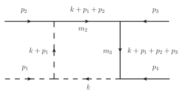
Nearly all the scalar four-point integrals mentioned above are evaluated with the dimensional regularization method[46]. An alternative way to extract singular parts in evaluating Feynman diagrams is loop regularization[50, 51], which has been successfully applied in some practical calculations in hadronic weak decays of $B$ mesons[52, 53, 54]. Motivated by the significant role played by the scalar one-loop four-point integral in reducing the tedious $N$-point($N\geq 5$) integrals to tractable ones, in this paper we will evaluate a typical infrared divergent scalar one-loop four-point integral as depicted in fig.1 using loop regularization method. The integral of fig.1, which corresponds to “Box $13$” of Ref.[40], is collinear divergent. As we know that the divergent structure of a amplitude is independent of the regularization scheme, but the expressions of the divergent part and the stable part may be distinct for different regularization scheme. Hence the purpose of the paper is, by a specific example, showing how the infrared divergent and infrared stable parts are extracted via loop regularization. We stress that in this paper we do not so ambitious as the aforementioned works on scalar one-loop four-point integrals which try to investigate the issue under various circumstances thoroughly, we only content ourselves on the diagram depicted in fig.1. In this sense we just present a case study on scalar one loop four-point integral by loop regularization. We hope that the results shed some light on the evaluation of scalar one loop four-point integrals, but also helpful in calculating some box diagram mediated decaying processes.

Before starting our evaluation, the following comments are in order.

(i)To perform the integrals over Feynman parameters, the Euler shift is adopted. Accordingly, two equations, i.e., Eq.(20) and Eq.(49), should be satisfied by the transforming parameters $\alpha$ and $\beta$. We assume that the two equations have two real roots, and one root of each equation lies in the range $(0,\,1)$ as stated in our evaluation. These requirements fix a kinematic allowed sector in the space spanned by the masses and external momentum, we call it sector I.

(ii)In our evaluation we need factorize 12 quadratic polynomials of $F$-type which are denoted by $F_{ij}(i=0,1;\,j=1,2,3)$ and of $G$-type which are denoted by $G_{ij}(i=0,1;\,j=1,2,3)$ into products of their roots. The $F$-type functions are in the denominator and the $G$-type functions are arguments of logarithms, the coefficients of the two type functions are formed by on-shell masses and masses of propagators as well as invariant combination of external momentum. It is obvious that the factorization should be careful since it depends on if the quadratic polynomials have two real roots. In other words, the validity of each factorization determines a kinematic sector where the quadratic polynomial has two real roots. Hence in all there are 12 kinematic sectors to be fixed, and the intersection of them is the kinematic sector where our evaluation is allowed, we call it as sector II. Figuring out sector II exactly is difficult in the complicated space established by the masses and external momentum. In order to get rid of the dilemma, we assume that there may be some kinematic sector in which all the factorizations are valid. A case-by-case analysis of the similar integrals one can refer to the appendix of Ref.[48] and appendix D of Ref.[49].

The overlap of sector I and II is the desired kinematic part where the results obtained in this paper can be correctly applied. We assume that there is some method by which the overlapping sector can be determined, although we do not find it explicitly in this paper. It is worth emphasizing that the required kinematic sector may be unphysical or even not existed, if it were this case, we just present a formal study on the infrared scalar one-loop four point integral.

The paper is organized as follows. After this short introduction we display some mathematical functions which are frequently used in our evaluation in section II. Then in Section III details of the evaluation and results are presented. Section IV contains our short summary. Some necessary formulae are listed in the appendix.

Figure 1: Scalar one-loop 4-point integral with one massless vertex. The dashed and solid lines are massless and massive, respectively. As usual all the external momenta are inward.

2 preliminaries

We define the following massive scalar one-loop 4-point integral with one massless vertex, as depicted in Fig.1

$$I=\int\frac{{\rm{d}}^{4}k}{(2\pi)^{4}}\frac{1}{\mathcal{D}_{1}\mathcal{D}_{2}\mathcal{D}_{3}\mathcal{D}_{4}},$$ (1)

where

$$\mathcal{D}_{1} = k^{2}+i\epsilon$$

$$\mathcal{D}_{2} = (k+p_{1})^{2}+i\epsilon$$

$$\mathcal{D}_{3} = (k+p_{1}+p_{2})^{2}-m_{2}^{2}+i\epsilon$$

$$\mathcal{D}_{4} = (k+p_{1}+p_{2}+p_{3})^{2}-m_{3}^{2}+i\epsilon,$$ (2)

The $i\epsilon$ will be systematically retained in our evaluation, $m_{2}$ and $m_{3}$ are the masses of the two massive internal lines. As usual we fix that the all the external momenta are inward, they are related by the energy conservation

$$p_{1}+p_{2}+p_{3}+p_{4}=0,$$ (3)

We assume that the four external momenta satisfy

$$p^{2}_{1}=0,\quad\quad p_{2}^{2}=\omega_{2}^{2},\quad\quad p_{3}^{2}=\omega_{3}^{2},\quad p_{4}^{2}=(p_{1}+p_{2}+p_{3})^{2}=\omega_{4}^{2},$$ (4)

for brevity we define

$$s_{ij}=p_{i}+p_{j}.$$ (5)

The results will be expressed in terms of logarithms and dilogarithms. As usual we choose the principal value of the logarithms lies in the negative axis, hence we find

$$\ln(x\pm i\epsilon)=\ln|x|\pm i\pi,\quad\quad x<0$$ (6)

In expanding logarithm of products one should take into account the convention[41]

$$\ln(ab)=\ln a+\ln b+\eta(a,b),$$ (7)

where the $\eta$ term is

$$\eta(a,b)=2\pi i\{\theta(-{\rm{Im}}\,a)\theta(-{\rm{Im}}\,b)\theta\big{(}{\rm{Im}}\,(ab)\big{)}-\theta({\rm{Im}}\,a)\theta({\rm{Im}}\,b)\theta\big{(}-{\rm{Im}}\,(ab)\big{)}\}.$$ (8)

following this rule it is easy to get

$$\ln(ab)=\ln a+\ln b,\quad\text{if ${\rm{Im}}(a)$ and ${\rm{Im}}(b)$ have different signs},$$

$$\ln\frac{a}{b}=\ln a-\ln b,\quad\text{if ${\rm{Im}}(a)$ and ${\rm{Im}}(b)$ have the same signs}.$$ (9)

As we know the dilogarithm develops an imaginary part for $x\geq 1$, then we have[45]

$${\rm{Li}}_{2}(x\pm i\epsilon)=-{\rm{Li}}_{2}\Big{(}\frac{1}{x}\Big{)}-\frac{1}{2}\ln^{2}x+\frac{\pi^{2}}{3}\pm i\pi\ln x,$$ (10)

Most of our results involve analytic continuation of dilogarithms of two variables

$${\rm{Li}}_{2}(1-x_{1}x_{2}),$$ (11)

this can be completed by the substitution[44, 37]

$${\rm{Li}}_{2}(1-x_{1}x_{2}) \rightarrow \mathcal{L}(x_{1},x_{2})$$ (12)

$$= {\rm{Li}}_{2}(1-x_{1}x_{2})+\eta(x_{1},x_{2})\ln(1-x_{1}x_{2}).$$

where $\eta(x_{1},x_{2})$ is given by Eq.(8).

3 calculation and results

3.1 basic formula

Firstly we notice that the first two denominators can be combined via Feynman parameterization

$$\frac{1}{(k^{2}+i\epsilon)[(k+p_{1})^{2}+i\epsilon]}=\int^{1}_{0}{\rm{d}}u\,\frac{1}{[(k+up_{1})^{2}+i\epsilon]^{2}},\,\quad\text{if}\quad p^{2}_{1}=0$$ (1)

Then primitive integral Eq.(1) becomes

$$I = \int\frac{{\rm{d}}^{4}k}{(2\pi)^{4}}\int^{1}_{0}{\rm{d}}u\,\frac{1}{[(k+up_{1})^{2}+i\epsilon]^{2}}$$ (2)

$$\times \frac{1}{[(k+p_{1}+p_{2})^{2}-m_{2}^{2}+i\epsilon][(k+p_{1}+p_{2}+p_{3})^{2}-m_{3}^{2}+i\epsilon]},$$

Then by using Feynman parameterization twice, Eq.(2) can be written in the form

$$I = 3\,!\int\frac{{\rm{d}}^{4}k}{(2\pi)^{4}}\int^{1}_{0}{\rm{d}}u\int^{1}_{0}{\rm{d}}x{\rm{d}}y{\rm{d}}z\,\delta(1-x-y-z)\,x$$ (3)

$$\times \Big{\{}x\big{[}(k+up_{1})^{2}+i\epsilon\big{]}+y\big{[}(k+p_{1}+p_{2})^{2}-m_{2}^{2}+i\epsilon\big{]}$$

$$+ z\big{[}(k+p_{1}+p_{2}+p_{3})^{2}-m_{3}^{2}+i\epsilon\big{]}\Big{\}}^{-4},$$

Sine there is infrared divergence in $I$, in order to carry out the integration over $k$, an appropriate regularization scheme must be employed. Instead of the most popular dimensional regularization, an alternative is loop regularization[50, 51]. According to the method, the loop momentum $k$ transforms as

$$k^{2}\rightarrow[k^{2}]_{l}=k^{2}-M_{l}^{2},$$

$$\int\frac{{\rm{d}}^{4}k}{(2\pi)^{4}}\rightarrow\int\Big{[}\frac{{\rm{d}}^{4}k}{(2\pi)^{4}}\Big{]}_{l}=\lim_{N,M_{i}^{2}\rightarrow\infty}\sum_{l=0}^{N}c^{N}_{l}\int\frac{d^{4}k}{(2\pi)^{4}},$$ (4)

which is constrained by

$$\lim_{N,M_{i}^{2}\rightarrow\infty}\sum_{l=0}^{N}c^{N}_{l}(M_{l}^{2})^{2}=0,\quad c_{0}^{N}=0\quad(i=0,1,...,N\,\,\text{and}\,\,n=0,1,..).$$ (5)

From Eq.(5) the coefficients $c_{l}^{N}$ can be worked out

$$c_{l}^{N}=(-1)^{l}\frac{N!}{l!(N-l)!},$$

and the regulator mass is given by

$$M^{2}_{l}=\mu^{2}_{s}+lM^{2}_{R},$$ (6)

Then it leads to the desired integration form over $k$

$$k^{2}\rightarrow k^{2}-\mu^{2}_{s}-lM^{2}_{R},$$

$$\int\frac{{\rm{d}}^{4}k}{(2\pi)^{4}}\rightarrow\lim_{N,M_{R}^{2}\rightarrow\infty}\sum_{l=0}^{N}(-1)^{l}\frac{N!}{l!(N-l)!}\int\frac{{\rm{d}}^{4}k}{(2\pi)^{4}}.$$ (7)

If there were only infrared divergence, when the integration over loop momentum is completed, terms involving $M_{R}$ will vanish after taking the limit, thus in this case it amounts to introduce a characteristic scale $\mu_{s}$ in the amplitudes. With this in mind, after the integration over $k$ is performed, we obtain

$$I=\frac{i}{(4\pi)^{2}}\int_{0}^{1}{\rm{d}}u\int_{0}^{1}{\rm{d}}x{\rm{d}}y{\rm{d}}z\,x\delta(1-x-y-z)\frac{1}{[Q(u,x,y,z)]^{2}},$$ (8)

where $Q$ is defined as

$$Q(u,x,y,z) = s_{12}^{2}y^{2}+\omega_{4}^{2}z^{2}+(s_{12}^{2}+\omega_{4}^{2}-\omega_{3}^{2})yz$$ (9)

$$+ \big{[}y(s_{12}^{2}-\omega_{2}^{2})+z(\omega_{4}^{2}-s_{23}^{2})\big{]}ux-y(s_{12}^{2}-m_{2}^{2})$$

$$- z(\omega_{4}^{2}-m_{3}^{2})-\mu_{s}^{2}-i\epsilon$$

The integration over $u$ is trivial thus we do it first

$$I=\frac{-i}{(4\pi)^{2}}\int_{0}^{1}{\rm{d}}x{\rm{d}}y{\rm{d}}z\,\delta(1-x-y-z)\frac{1}{B(y,z)}\Big{[}\frac{1}{Q(1,x,y,z)}-\frac{1}{Q(0,x,y,z)}\Big{]},$$ (10)

where

$$B(y,z)=y(s_{12}^{2}-\omega_{2}^{2})+z(\omega_{4}^{2}-s_{23}^{2}).$$ (11)

The integration over $z$ can be performed immediately, it leads to

$$I = \frac{-i}{(4\pi)^{2}}\int_{0}^{1}{\rm{d}}x\int_{0}^{1-x}{\rm{d}}y\,\frac{1}{B(y,1-x-y)}$$ (12)

$$\times \Big{[}\frac{1}{Q(1,x,y,1-x-y)}-\frac{1}{Q(0,x,y,1-x-y)}\Big{]}$$

To proceed we make the following transformation on $x$ and $y$

$$x=1-x^{\prime},\quad\quad y=x^{\prime}-y^{\prime}$$ (13)

this yields a convenient form for Eq.(12)

$$I=\frac{-i}{(4\pi)^{2}}\int_{0}^{1}{\rm{d}}x^{\prime}\int_{0}^{x^{\prime}}{\rm{d}}y^{\prime}\,\frac{1}{C(x^{\prime},y^{\prime})}\Big{[}\frac{1}{W_{1}(x^{\prime},y^{\prime})}-\frac{1}{W_{0}(x^{\prime},y^{\prime})}\Big{]},$$ (14)

where

$$C(x^{\prime},y^{\prime}) = (s_{12}^{2}-\omega_{2}^{2})x^{\prime}+(s_{13}^{2}-\omega_{3}^{2})y^{\prime},$$

$$W_{1}(x^{\prime},y^{\prime}) = \omega_{2}^{2}x^{\prime 2}+\omega_{3}^{2}y^{\prime 2}+(s_{12}^{2}-\omega_{2}^{2}-\omega_{3}^{2})x^{\prime}y^{\prime}-\omega_{2}^{2}x^{\prime},$$

$$+ (m_{3}^{2}-m_{2}^{2}-s_{23}^{2}+\omega_{2}^{2})y^{\prime}-\mu_{s}^{2}-i\epsilon,$$

$$W_{0}(x^{\prime},y^{\prime}) = s_{12}^{2}x^{\prime 2}+\omega_{3}^{2}y^{\prime 2}+(\omega_{4}^{2}-s_{12}^{2}-\omega_{3}^{2})x^{\prime}y^{\prime}$$ (15)

$$- (s_{12}^{2}-m_{2}^{2})x^{\prime}+(s_{12}^{2}-m_{2}^{2}-\omega_{4}^{2}+m_{3}^{2})y^{\prime}-\mu_{s}^{2}-i\epsilon.$$

For later convenience we split $I$ into two parts

$$I=I_{1}+I_{0},$$ (16)

where the two components are

$$I_{1} = \frac{-i}{(4\pi)^{2}}\int_{0}^{1}{\rm{d}}x^{\prime}\int_{0}^{x^{\prime}}{\rm{d}}y^{\prime}\,\frac{1}{C(x^{\prime},y^{\prime})W_{1}(x^{\prime},y^{\prime})}$$

$$I_{0} = \frac{i}{(4\pi)^{2}}\int_{0}^{1}{\rm{d}}x^{\prime}\int_{0}^{x^{\prime}}{\rm{d}}y^{\prime}\,\frac{1}{C(x^{\prime},y^{\prime})W_{0}(x^{\prime},y^{\prime})}$$ (17)

We will evaluate $I_{1}$ and $I_{0}$ in the forthcoming two subsections, respectively.

3.2 evaluation of $I_{1}$

Since the denominator $W_{1}$ is quadratic both in $x^{\prime}$ and $y^{\prime}$, in order to cope with terms involving $x^{2}$, we perform the so-called Euler shift on $y^{\prime}$

$$y^{\prime}=\rho+\alpha x^{\prime}$$ (18)

such that

$$\int_{0}^{1}{\rm{d}}x^{\prime}\int_{0}^{x^{\prime}}{\rm{d}}y^{\prime}=\int_{0}^{1-\alpha}{\rm{d}}\rho\int_{\rho/(1-\alpha)}^{1}{\rm{d}}x^{\prime}-\int_{0}^{-\alpha}{\rm{d}}\rho\int_{-\rho/\alpha}^{1}{\rm{d}}x^{\prime}$$ (19)

where the parameter $\alpha$ is chosen to obey the condition

$$\omega_{3}^{2}\alpha^{2}+\alpha(s_{23}^{2}-\omega_{2}^{2}-\omega_{3}^{2})+\omega_{2}^{2}=0$$ (20)

From Eq.(20) we find

$$\alpha = \frac{1}{2\omega_{3}^{2}}\Big{[}-(s_{23}^{2}-\omega_{2}^{2}-\omega_{3}^{2})\pm\lambda^{1/2}(s_{23}^{2},\omega_{2}^{2},\omega_{3}^{2})\Big{]},$$ (21)

where $\lambda(x,y,z)$ is the well-known K$\ddot{a}$llen function

$$\lambda(x,y,z)=(x+y+z)^{2}-2xy-2yz-2xz,$$ (22)

In our evaluation we take

$$\alpha=\frac{1}{2\omega_{3}^{2}}\Big{[}-(s_{23}^{2}-\omega_{2}^{2}-\omega_{3}^{2})+\lambda^{1/2}(s_{23}^{2},\omega_{2}^{2},\omega_{3}^{2})\Big{]}.$$ (23)

and assume $0<\alpha<1$. According to Eq.(20), all the $x^{\prime 2}$-dependent terms vanish, now $W_{1}$ is linear in $x^{\prime}$, we denote it as

$$Y_{1}(x^{\prime},\rho)=f_{1}(\rho)x^{\prime}+f_{2}(\rho)$$ (24)

where $f_{1}$ and $f_{2}$ only depend on $\rho$, the explicit expressions are

$$f_{1}(\rho) = A_{1}\rho+B_{1},$$

$$f_{2}(\rho) = A_{2}\rho^{2}+B_{2}\rho-\mu_{s}^{2}-i\epsilon,$$ (25)

All the coefficients in Eq.(25) are constants which are formed by on-shell masses in Eq.(LABEL:onshellmasses) and propagator masses $m_{i}(i=2,3)$ as well as combinations of external momentum $s_{ij}$ in Eq.(5)

$$A_{1} = s_{23}^{2}+(2\alpha-1)\omega_{3}^{2}-\omega_{2}^{2},$$

$$B_{1} = (m_{2}^{2}-\omega_{2}^{2})+\alpha(m_{3}^{2}-m_{2}^{2}+\omega_{2}^{2}-s_{23}^{2}),$$

$$A_{2} = \omega_{3}^{2},$$

$$B_{2} = m_{3}^{2}-m_{2}^{2}+\omega_{2}^{2}-s_{23}^{2},$$

$$D_{1} = s_{13}^{2}-\omega_{3}^{2}.$$ (26)

Under the transformation in Eq.(18), the function $C(x^{\prime},y^{\prime})$ besomes

$$X(x^{\prime},\rho)=g_{0}(\alpha)x^{\prime}+g_{1}(\rho)$$ (27)

where $g_{0}(\alpha)$ is constant and $g_{1}(\rho)$ is linear in $\rho$

$$g_{0}(\alpha)=s_{12}^{2}-\omega_{2}^{2}+\alpha(s_{13}^{2}-\omega_{3}^{2}),\quad g_{1}(\rho)=D_{1}\rho$$ (28)

This yields a compact form for $I_{1}$, which reads

$$I_{1} = \frac{-i}{(4\pi)^{2}}\Big{[}\int_{0}^{1-\alpha}{\rm{d}}\rho\int_{\rho/(1-\alpha)}^{1}{\rm{d}}x^{\prime}-\int_{0}^{-\alpha}{\rm{d}}\rho\int_{-\rho/\alpha}^{1}{\rm{d}}x^{\prime}\Big{]}\frac{1}{(g_{0}x^{\prime}+g_{1})(f_{1}x^{\prime}+f_{2})}$$ (29)

$$= \frac{-i}{(4\pi)^{2}}\Big{[}\int_{0}^{1-\alpha}{\rm{d}}\rho\int_{\rho/(1-\alpha)}^{1}{\rm{d}}x^{\prime}-\int_{0}^{-\alpha}{\rm{d}}\rho\int_{-\rho/\alpha}^{1}{\rm{d}}x^{\prime}\Big{]}\frac{1}{g_{0}f_{2}-g_{1}f_{1}}$$

$$\times \Big{(}\frac{g_{0}}{g_{0}x^{\prime}+g_{1}}-\frac{f_{1}}{f_{1}x^{\prime}+f_{2}}\Big{)}$$

$$= I_{A}+I_{B}$$

where we have split $I_{1}$ into two parts

$$I_{A} = \frac{-i}{(4\pi)^{2}}\int_{0}^{1-\alpha}{\rm{d}}\rho\int_{\rho/(1-\alpha)}^{1}{\rm{d}}x^{\prime}\frac{1}{g_{0}f_{2}-g_{1}f_{1}}\Big{(}\frac{g_{0}}{g_{0}x^{\prime}+g_{1}}-\frac{f_{1}}{f_{1}x^{\prime}+f_{2}}\Big{)},$$ (30)

$$I_{B} = \frac{i}{(4\pi)^{2}}\int_{0}^{-\alpha}{\rm{d}}\rho\int_{-\rho/\alpha}^{1}{\rm{d}}x^{\prime}\frac{1}{g_{0}f_{2}-g_{1}f_{1}}\Big{(}\frac{g_{0}}{g_{0}x^{\prime}+g_{1}}-\frac{f_{1}}{f_{1}x^{\prime}+f_{2}}\Big{)}.$$ (31)

The integration over $x^{\prime}$ in Eq.(30) and Eq.(31) is elementary, we can carry out it immediately, the results are

$$I_{A} = \frac{-i}{(4\pi)^{2}}\int_{0}^{1-\alpha}{\rm{d}}\rho\frac{1}{g_{0}f_{2}-g_{1}f_{1}}\Big{[}\ln\Big{(}g_{0}+g_{1}\Big{)}-\ln\Big{(}\frac{\rho}{1-\alpha}\,g_{0}+g_{1}\Big{)}$$ (32)

$$- \ln\Big{(}f_{1}+f_{2}\Big{)}+\ln\Big{(}\frac{\rho}{1-\alpha}\,f_{1}+f_{2}\Big{)}\Big{]},$$

and

$$I_{B} = \frac{i}{(4\pi)^{2}}\int_{0}^{-\alpha}{\rm{d}}\rho\frac{1}{g_{0}f_{2}-g_{1}f_{1}}\Big{[}\ln\Big{(}g_{0}+g_{1}\Big{)}-\ln\Big{(}-\frac{\rho}{\alpha}\,g_{0}+g_{1}\Big{)}$$ (33)

$$- \ln\Big{(}f_{1}+f_{2}\Big{)}+\ln\Big{(}-\frac{\rho}{\alpha}\,f_{1}+f_{2}\Big{)}\Big{]}.$$

Then we divide the upper limit of the integral of $I_{A}$ into two parts

$$I_{1} = \frac{-i}{(4\pi)^{2}}\Big{(}\int_{0}^{1}{\rm{d}}\rho+\int_{0}^{-\alpha}{\rm{d}}\rho\Big{)}\frac{1}{g_{0}f_{2}-g_{1}f_{1}}\Big{[}\ln\Big{(}g_{0}+g_{1}\Big{)}-\ln\Big{(}\frac{\rho}{1-\alpha}\,g_{0}+g_{1}\Big{)}$$ (34)

$$- \ln\Big{(}f_{1}+f_{2}\Big{)}+\ln\Big{(}\frac{\rho}{1-\alpha}\,f_{1}+f_{2}\Big{)}\Big{]},$$

Combining with Eq.(33), after some cancelation we find

$$I_{1}=\frac{-i}{(4\pi)^{2}}(I_{11}+I_{12}+I_{13})$$ (35)

The first component $I_{11}$ is given by

$$I_{11} = \int_{0}^{1}{\rm{d}}\rho\,\frac{1}{g_{0}f_{2}-g_{1}f_{1}}\Big{[}\ln(g_{0}+g_{1})-\ln(f_{1}+f_{2})\Big{]}$$ (36)

$$= \int_{0}^{1}{\rm{d}}\rho\frac{1}{F_{11}(\rho)}\Big{[}\ln(g_{0}+g_{1})-\ln G_{11}(\rho)\Big{]},$$

where

$$F_{11}(\rho) = (A_{2}g_{0}-A_{1}D_{1})\rho^{2}+(B_{2}g_{0}-B_{1}D_{1})\rho-g_{0}(\mu_{s}^{2}+i\epsilon)$$

$$G_{11}(\rho) = A_{2}\rho^{2}+(A_{1}+B_{2})\rho+B_{1}-\mu_{s}^{2}-i\epsilon.$$ (37)

The other two components are

$$I_{12} = \int_{0}^{1-\alpha}{\rm{d}}\rho\,\frac{1}{g_{0}f_{2}-g_{1}f_{1}}\Big{[}-\ln\Big{(}\frac{\rho}{1-\alpha}g_{0}+g_{1}\Big{)}+\ln\Big{(}\frac{\rho}{1-\alpha}f_{1}+f_{2}\Big{)}\Big{]},$$ (38)

$$I_{13} = \int_{0}^{-\alpha}{\rm{d}}\rho\,\frac{1}{g_{0}f_{2}-g_{1}f_{1}}\Big{[}\ln\Big{(}-\frac{\rho}{\alpha}g_{0}+g_{1}\Big{)}-\ln\Big{(}-\frac{\rho}{\alpha}f_{1}+f_{2}\Big{)}\Big{]}.$$ (39)

In order to regularize the upper limit of the integral in Eq.(38, we make the following variable substitution

$$\rho=(1-\alpha)\xi,$$ (40)

without confusion, we relabel $\xi$ as $\rho$, then the integral takes the form

$$I_{12}=(1-\alpha)\int_{0}^{1}{\rm{d}}\rho\,\frac{1}{F_{12}(\rho)}\Big{\{}-\ln\Big{[}\Big{(}g_{0}+(1-\alpha)D_{1}\Big{)}\rho\Big{]}+\ln G_{12}(\rho)\Big{\}},$$ (41)

where

$$F_{12}(\rho) = (1-\alpha)^{2}(A_{2}g_{0}-A_{1}D_{1})\rho^{2}+(1-\alpha)(B_{2}g_{0}-B_{1}D_{1})\rho-g_{0}(\mu_{s}^{2}+i\epsilon),$$

$$G_{12}(\rho) = (1-\alpha)[A_{1}+(1-\alpha)A_{2}]\rho^{2}+[B_{1}+(1-\alpha)B_{2}]\rho-\mu_{s}^{2}-i\epsilon,$$ (42)

Similarly, we make the following transformation in Eq.(39)

$$\rho=-\alpha\xi,$$ (43)

and relabel $\xi$ as $\rho$, this leads to

$$I_{13}=-\alpha\int_{0}^{1}{\rm{d}}\rho\,\frac{1}{F_{13}(\rho)}\Big{\{}\ln\Big{[}(g_{0}-D_{1}\alpha)\rho\Big{]}-\ln G_{13}(\rho)\Big{\}},$$ (44)

where

$$F_{13}(\rho) = \alpha^{2}(A_{2}g_{0}-A_{1}D_{1})\rho^{2}+\alpha(B_{1}D_{1}-B_{2}g_{0})\rho-g_{0}(\mu_{s}^{2}+i\epsilon)$$

$$G_{13}(\rho) = \alpha(\alpha A_{2}-A_{1})\rho^{2}-(\alpha B_{2}-B_{1})\rho-\mu_{s}^{2}-i\epsilon$$ (45)

The details of evaluating of $I_{11}$, $I_{12}$ and $I_{13}$ are presented in appendix C.

3.3 evaluation of $I_{0}$

The original expression of $I_{0}$ is

$$I_{0} = \frac{i}{(4\pi)^{2}}\int_{0}^{1}{\rm{d}}x^{\prime}\int_{0}^{x^{\prime}}{\rm{d}}y^{\prime}\,\frac{1}{C(x^{\prime},y^{\prime})W_{0}(x^{\prime},y^{\prime})},$$ (46)

To eliminate the awkward term depending on $x^{\prime 2}$, we also make the Euler shift on $y^{\prime}$

$$y^{\prime}=\rho+\beta x^{\prime}$$ (47)

such that

$$\int_{0}^{1}{\rm{d}}x^{\prime}\int_{0}^{x^{\prime}}{\rm{d}}y^{\prime}=\int_{0}^{1-\beta}{\rm{d}}\rho\int_{\rho/(1-\beta)}^{1}{\rm{d}}x^{\prime}-\int_{0}^{-\beta}{\rm{d}}\rho\int_{-\rho/\beta}^{1}{\rm{d}}x^{\prime}$$ (48)

where $\beta$ is chosen to obey the condition

$$\omega_{3}^{2}\beta^{2}+(\omega_{4}^{2}-s_{12}^{2}-\omega_{3}^{2})\beta+s_{12}^{2}=0$$ (49)

which renders that all the $x^{\prime 2}$-dependent terms vanish. The roots of Eq.(49) are

$$\beta=\frac{1}{2\omega_{3}^{2}}\Big{[}-(\omega_{4}^{2}-s_{12}^{2}-\omega_{3}^{2})\pm\lambda^{1/2}(\omega_{4}^{2},s_{12}^{2},\omega_{3}^{2})\,\Big{]}$$ (50)

where $\lambda(x,y,z)$ is the Kallen function defined in Eq.(22). In our evaluation we take

$$\beta=\frac{1}{2\omega_{3}^{2}}\Big{[}-(\omega_{4}^{2}-s_{12}^{2}-\omega_{3}^{2})+\lambda^{1/2}(\omega_{4}^{2},s_{12}^{2},\omega_{3}^{2})\,\Big{]}.$$ (51)

and assume $0<\beta<1$. Accordingly, $W_{0}$ is linear in $x^{\prime}$, we denote it as

$$Y_{0}(x^{\prime},\rho)=h_{1}(\rho)x^{\prime}+h_{2}(\rho),$$ (52)

where the two functions $h_{1}(\rho)$ and $h_{2}(\rho)$ only depend on $\rho$, they are given by

$$h_{1}(\rho) = K_{1}\rho+N_{1}$$

$$h_{2}(\rho) = K_{2}\rho^{2}+N_{2}\rho-\mu_{s}^{2}-i\epsilon,$$ (53)

all the coefficients in Eq.(53) are constants

$$K_{1} = 2(\beta-1)\omega_{3}^{2}+s_{13}^{2}+s_{23}^{2}-\omega_{2}^{2},$$

$$N_{1} = (\beta-1)(s_{12}^{2}-m_{2}^{2})-\beta(\omega_{4}^{2}-m_{3}^{2}),$$

$$K_{2} = \omega_{3}^{2},$$

$$N_{2} = s_{12}^{2}-m_{2}^{2}-\omega_{4}^{2}+m_{3}^{2}.$$ (54)

While $C(x^{\prime},y^{\prime})$ transform into

$$X(x^{\prime},\rho)=g_{0}(\beta)x^{\prime}+g_{1}(\rho),$$ (55)

where $g_{0}(\beta)$ and $g_{1}(\rho)$ is given by

$$g_{0}(\beta) = s_{12}^{2}-\omega_{2}^{2}+\beta(s_{13}^{2}-\omega_{3}^{2}),$$

$$g_{1}(\rho) = D_{1}\rho,$$ (56)

Then we rewrite $I_{0}$ in a compact form

$$I_{0} = \frac{i}{(4\pi)^{2}}\Big{[}\int_{0}^{1-\beta}{\rm{d}}\rho\int_{\rho/(1-\beta)}^{1}{\rm{d}}x^{\prime}-\int_{0}^{-\beta}{\rm{d}}\rho\int_{-\rho/\beta}^{1}{\rm{d}}x^{\prime}\Big{]}\frac{1}{(g_{0}x^{\prime}+g_{1})(h_{1}x^{\prime}+h_{2})}$$ (57)

$$= \frac{-i}{(4\pi)^{2}}\Big{[}\int_{0}^{1-\beta}{\rm{d}}\rho\int_{\rho/(1-\beta)}^{1}{\rm{d}}x^{\prime}-\int_{0}^{-\beta}{\rm{d}}\rho\int_{-\rho/\beta}^{1}{\rm{d}}x^{\prime}\Big{]}$$

$$\times \frac{1}{g_{0}h_{2}-g_{1}h_{1}}\Big{(}\frac{g_{0}}{g_{0}x^{\prime}+g_{1}}-\frac{h_{1}}{h_{1}x^{\prime}+h_{2}}\Big{)}.$$

After the trivial integration over $x^{\prime}$ is performed, we find

$$I_{0}=I_{C}+I_{D},$$ (58)

where

$$I_{C} = \frac{i}{(4\pi)^{2}}\int_{0}^{1-\beta}{\rm{d}}\rho\,\frac{1}{g_{0}h_{2}-g_{1}h_{1}}\Big{[}\ln\Big{(}g_{0}+g_{1}\Big{)}-\ln\Big{(}\frac{\rho}{1-\beta}g_{0}+g_{1}\Big{)}$$ (59)

$$- \ln\Big{(}h_{1}+h_{2}\Big{)}+\ln\Big{(}\frac{\rho}{1-\beta}h_{1}+h_{2}\Big{)}\Big{]}$$

$$= \frac{-i}{(4\pi)^{2}}\Big{(}\int_{0}^{1}{\rm{d}}\rho\,+\int_{0}^{-\beta}{\rm{d}}\rho\Big{)}\frac{1}{g_{0}h_{2}-g_{1}h_{1}}\Big{[}\ln\Big{(}g_{0}+g_{1}\Big{)}-\ln\Big{(}\frac{\rho}{1-\beta}g_{0}+g_{1}\Big{)}$$

$$- \ln\Big{(}h_{1}+h_{2}\Big{)}+\ln\Big{(}\frac{\rho}{1-\beta}h_{1}+h_{2}\Big{)}\Big{]},$$

and

$$I_{D} = \frac{i}{(4\pi)^{2}}\int_{0}^{-\beta}{\rm{d}}\rho\,\frac{1}{g_{0}h_{2}-g_{1}h_{1}}$$ (60)

$$\times \Big{[}\ln(g_{0}+g_{1})-\ln(-\frac{\rho}{\beta}g_{0}+g_{1})-\ln(h_{1}+h_{2})+\ln(-\frac{\rho}{\beta}h_{1}+h_{2})\Big{]}.$$

After some cancelation, we have

$$I_{0}=\frac{i}{(4\pi)^{2}}(I_{01}+I_{02}+I_{03}),$$ (61)

The first component is

$$I_{01} = \int_{0}^{1}{\rm{d}}\rho\,\frac{1}{g_{0}h_{2}-g_{1}h_{1}}\Big{[}\ln(g_{0}+g_{1})-\ln(h_{1}+h_{2})\Big{]}$$ (62)

$$= \int_{0}^{1}{\rm{d}}u\,\frac{1}{F_{01}(\rho)}\Big{[}\ln\Big{(}D_{1}u+g_{0}\Big{)}-\ln G_{01}(\rho)\Big{]},$$

where

$$F_{01}(\rho) = (K_{2}g_{0}-K_{1}D_{1})\rho^{2}+(g_{0}N_{2}-N_{1}D_{1})\rho-g_{0}(\mu_{s}^{2}+i\epsilon)$$

$$G_{01}(\rho) = K_{2}\rho^{2}+(K_{1}+N_{2})\rho+N_{1}-\mu_{s}^{2}-i\epsilon.$$ (63)

The second component is

$$I_{02}=\int_{0}^{1-\beta}{\rm{d}}\rho\,\frac{1}{g_{0}h_{2}-g_{1}h_{1}}\Big{[}-\ln\Big{(}\frac{\rho}{1-\beta}g_{0}+g_{1}\Big{)}+\ln\Big{(}\frac{\rho}{1-\beta}h_{1}+h_{2}\Big{)}\Big{]},$$ (64)

We make the following transform on $I_{02}$

$$\rho=(1-\beta)\xi,$$ (65)

and relabel $\xi$ as $\rho$, we obtain

$$I_{02}=(1-\beta)\int_{0}^{1}{\rm{d}}\rho\,\frac{1}{F_{02}(\rho)}\Big{\{}-\ln\Big{[}\Big{(}g_{0}+(1-\beta)D_{1}\Big{)}\rho\Big{]}+\ln G_{02}(\rho)\Big{\}},$$ (66)

where

$$F_{02}(\rho) = (1-\beta)^{2}(K_{2}g_{0}-K_{1}D_{1})\rho^{2}-(1-\beta)(N_{1}D_{1}-N_{2}g_{0})\rho-g_{0}(\mu_{s}^{2}+i\epsilon),$$

$$G_{02}(\rho) = (1-\beta)[K_{1}+(1-\beta)K_{2}]\rho^{2}+[N_{1}+(1-\beta)N_{2}]\rho-\mu_{s}^{2}-i\epsilon.$$ (67)

The last component is

$$I_{03}=\int_{0}^{-\beta}{\rm{d}}\rho\,\frac{1}{g_{0}h_{2}-g_{1}h_{1}}\Big{[}\ln\Big{(}-\frac{\rho}{\beta}g_{0}+g_{1}\Big{)}-\ln\Big{(}-\frac{u}{\beta}h_{1}+h_{2}\Big{)}\Big{]},$$ (68)

We make the following transformation

$$\rho=-\beta\xi,$$ (69)

and relabel $\xi$ as $\rho$, the

$$I_{03}=-\beta\int_{0}^{1}{\rm{d}}\rho\,\frac{1}{F_{03}(\rho)}\Big{\{}\ln\Big{[}\Big{(}g_{0}-\beta D_{1}\Big{)}\rho\Big{]}-\ln G_{03}(\rho)\Big{\}}$$ (70)

where

$$F_{03}(\rho) = \beta^{2}(K_{2}g_{0}-K_{1}D_{1})\rho^{2}+\beta(N_{1}D_{1}-N_{2}g_{0})\rho-g_{0}(\mu_{s}^{2}+i\epsilon),$$

$$G_{03}(\rho) = \beta(\beta K_{2}-K_{1})\rho^{2}-(\beta N_{2}-N_{1})\rho-\mu_{s}^{2}-i\epsilon.$$ (71)

The details of evaluating of $I_{01}$, $I_{02}$ and $I_{03}$ are given in appendix D.

3.4 results and discussions

Collecting the components in the appendix C and D, we arrive at the final results for $I$

$$I=I_{1}+I_{2},$$ (72)

where the manifest expressions of $I_{1}$ and $I_{1}$ are

$$I_{1} = \frac{-i}{(4\pi)^{2}}(I_{11}+I_{12}+I_{13})$$ (73)

$$= \frac{-i}{(4\pi)^{2}}\frac{1}{a_{1}[\rho^{(1)}_{+}-\rho^{(1)}_{-}]}\Big{\{}\ln\frac{\lambda_{1}^{2}}{\mu_{s}^{2}}+\ln\frac{\lambda_{1}^{2}}{\mu_{s}^{2}}\Big{[}\ln\alpha-\ln(1-\alpha)\Big{]}+\ln\Big{|}1-\frac{\lambda^{2}}{\mu_{s}^{2}}\Big{|}\ln\frac{g_{0}+D_{1}\rho^{(1)}_{+}}{G_{11}(1)}$$

$$- \ln\Big{|}1-\frac{(1-\alpha)\lambda^{2}}{\mu_{s}^{2}}\Big{|}\ln\frac{g_{0}+(1-\alpha)D_{1}}{G_{12}(1)}+\ln\Big{|}1+\frac{\alpha\lambda_{1}^{2}}{\mu_{s}^{2}}\Big{|}\ln\frac{g_{0}-\alpha D_{1}}{G_{13}(1)}+i\pi\ln\frac{\lambda_{1}^{2}}{\mu_{s}^{2}}$$

$$+ i\pi\Big{[}\ln\frac{g_{0}+D_{1}\rho^{(1)}_{+}}{G_{11}(1)}-\ln\frac{g_{0}+(1-\alpha)D_{1}}{G_{12}(1)}-\ln(1-\alpha)\Big{]}-\frac{\pi^{2}}{6}+\frac{1}{2}\Big{[}\ln^{2}\alpha-\ln^{2}(1-\alpha)\Big{]}$$

$$- \ln\Big{[}1-\frac{1}{\rho^{(1)}_{-}}\Big{]}\ln\frac{g_{0}+D_{1}\rho^{(1)}_{+}}{G_{11}(1)}+\ln\Big{[}1-\frac{1-\alpha}{\rho^{(1)}_{-}}\Big{]}\ln\frac{g_{0}+(1-\alpha)D_{1}}{G_{12}(1)}$$

$$- \ln\Big{[}1+\frac{\alpha}{\rho^{(1)}_{-}}\Big{]}\ln\frac{g_{0}-\alpha D_{1}}{G_{13}(1)}+{\rm{Li}}_{2}\Big{[}\frac{-D_{1}\rho^{(1)}_{+}}{-D_{1}\rho^{(1)}_{+}-g_{0}}\Big{]}-{\rm{Li}}_{2}\Big{[}\frac{D_{1}(1-\rho^{(1)}_{+})}{-D_{1}\rho^{(1)}_{+}-g_{0}}\Big{]}$$

$$- {\rm{Li}}_{2}\Big{[}\frac{-D_{1}\rho^{(1)}_{-}}{-D_{1}\rho^{(1)}_{-}-g_{0}}\Big{]}+{\rm{Li}}_{2}\Big{[}\frac{D_{1}(1-\rho^{(1)}_{-})}{-D_{1}\rho^{(1)}_{-}-g_{0}}\Big{]}$$

$$+ 2{\rm{Li}}_{2}(\frac{\mu_{s}^{2}}{\lambda_{1}^{2}})+{\rm{Li}}_{2}\Big{[}1-\frac{\rho^{(1)}_{+}}{1-\rho^{(1)}_{+}}\frac{\rho^{(1)}_{11}}{1-\rho^{(1)}_{11}}\Big{]}+{\rm{Li}}_{2}\Big{[}1-\frac{\rho^{(1)}_{+}}{1-\rho^{(1)}_{+}}\frac{\rho^{(2)}_{11}}{1-\rho^{(2)}_{11}}\Big{]}$$

$$+ 2{\rm{Li}}_{2}\Big{[}\frac{1}{\rho^{(1)}_{-}}\Big{]}-{\rm{Li}}_{2}\Big{[}1-\frac{\rho^{(1)}_{-}}{1-\rho^{(1)}_{-}}\frac{\rho^{(1)}_{11}}{1-\rho^{(1)}_{11}}\Big{]}-{\rm{Li}}_{2}\Big{[}1-\frac{\rho^{(1)}_{-}}{1-\rho^{(1)}_{-}}\frac{\rho^{(2)}_{11}}{1-\rho^{(2)}_{11}}\Big{]}$$

$$- {\rm{Li}}_{2}\Big{[}\frac{\mu_{s}^{2}}{(1-\alpha)\lambda_{1}^{2}}\Big{]}-{\rm{Li}}_{2}\Big{[}1-\frac{\rho^{(1)}_{+}}{1-\alpha-\rho^{(1)}_{+}}\frac{\rho^{(1)}_{12}}{1-\rho^{(1)}_{12}}\Big{]}-{\rm{Li}}_{2}\Big{[}1-\frac{\rho^{(1)}_{+}}{1-\alpha-\rho^{(1)}_{+}}\frac{\rho^{(2)}_{12}}{1-\rho^{(2)}_{12}}\Big{]}$$

$$- {\rm{Li}}_{2}\Big{[}\frac{1-\alpha}{\rho^{(1)}_{-}}\Big{]}+{\rm{Li}}_{2}\Big{[}1-\frac{\rho^{(1)}_{-}}{1-\alpha-\rho^{(1)}_{-}}\frac{\rho^{(1)}_{12}}{1-\rho^{(1)}_{12}}\Big{]}+{\rm{Li}}_{2}\Big{[}1-\frac{\rho^{(1)}_{-}}{1-\alpha-\rho^{(1)}_{-}}\frac{\rho^{(2)}_{12}}{1-\rho^{(2)}_{12}}\Big{]}$$

$$+ {\rm{Li}}_{2}\Big{[}-\frac{\mu_{s}^{2}}{\alpha\lambda_{1}^{2}}\Big{]}+{\rm{Li}}_{2}\Big{[}1+\frac{\rho^{(1)}_{+}}{\alpha+\rho^{(1)}_{+}}\frac{\rho^{(1)}_{13}}{1-\rho^{(1)}_{13}}\Big{]}+{\rm{Li}}_{2}\Big{[}1+\frac{\rho^{(1)}_{+}}{\alpha+\rho^{(1)}_{+}}\frac{\rho^{(2)}_{13}}{1-\rho^{(2)}_{13}}\Big{]}$$

$$+ {\rm{Li}}_{2}\Big{[}-\frac{\alpha}{\rho^{(1)}_{-}}\Big{]}-{\rm{Li}}_{2}\Big{[}1+\frac{\rho^{(1)}_{-}}{\alpha+\rho^{(1)}_{-}}\frac{\rho^{(1)}_{13}}{1-\rho^{(1)}_{13}}\Big{]}-{\rm{Li}}_{2}\Big{[}1+\frac{\rho^{(1)}_{-}}{\alpha+\rho^{(1)}_{-}}\frac{\rho^{(2)}_{13}}{1-\rho^{(2)}_{13}}\Big{]}\Big{\}},$$

and

$$I_{0} = \frac{i}{(4\pi)^{2}}(I_{01}+I_{02}+I_{03})$$ (74)

$$= \frac{i}{(4\pi)^{2}}\frac{1}{a_{0}[\rho^{(0)}_{+}-\rho^{(0)}_{-}]}\Big{\{}\ln^{2}\frac{\lambda_{0}^{2}}{\mu_{s}^{2}}+\ln\frac{\lambda_{0}^{2}}{\mu_{s}^{2}}\Big{[}\ln\beta-\ln(1-\beta)\Big{]}+\ln\Big{|}1-\frac{\lambda_{0}^{2}}{\mu_{s}^{2}}\Big{|}\ln\frac{g_{0}+D_{1}\rho_{+}^{(0)}}{G_{01}(1)}$$

$$- \ln\Big{|}1-\frac{(1-\beta)\lambda_{0}^{2}}{\mu_{s}^{2}}\Big{|}\ln\frac{g_{0}+(1-\beta)D_{1}}{G_{02}(1)}+\ln\Big{|}1+\frac{\beta\lambda_{0}^{2}}{\mu_{s}^{2}}\Big{|}\ln\frac{g_{0}-\beta D_{1}}{G_{03}(1)}$$

$$+ i\pi\ln\frac{\lambda_{0}^{2}}{\mu_{s}^{2}}+i\pi\Big{[}\ln\frac{g_{0}+D_{1}\rho_{+}^{(0)}}{G_{01}(1)}-\ln\frac{g_{0}+(1-\beta)D_{1}}{G_{02}(1)}-\ln(1-\beta)\Big{]}$$

$$- \frac{\pi^{2}}{6}+\frac{1}{2}\Big{[}\ln^{2}\beta-\ln^{2}(1-\beta)\Big{]}-\ln\Big{(}1-\frac{1}{\rho_{-}^{(0)}}\Big{)}\ln\frac{g_{0}+D_{1}\rho_{-}^{(0)}}{G_{01}(1)}$$

$$+ \ln\Big{(}1-\frac{1-\beta}{\rho_{-}^{(0)}}\Big{)}\ln\frac{g_{0}+(1-\beta)D_{1}}{G_{02}(1)}-\ln\Big{(}1+\frac{\beta}{\rho_{-}^{(0)}}\Big{)}\ln\frac{g_{0}-\beta D_{1}}{G_{03}(1)}$$

$$+ {\rm{Li}}_{2}\Big{[}\frac{-D_{1}\rho^{(0)}_{+}}{-D_{1}\rho^{(0)}_{+}-g_{0}}\Big{]}-{\rm{Li}}_{2}\Big{[}\frac{D_{1}(1-\rho^{(0)}_{+})}{-D_{1}\rho^{(0)}_{+}-g_{0}}\Big{]}$$

$$- {\rm{Li}}_{2}\Big{[}\frac{-D_{1}\rho^{(0)}_{-}}{-D_{1}\rho^{(0)}_{-}-g_{0}}\Big{]}+{\rm{Li}}_{2}\Big{[}\frac{D_{1}(1-\rho^{(0)}_{-})}{-D_{1}\rho^{(0)}_{-}-g_{0}}\Big{]}$$

$$+ 2{\rm{Li}}_{2}(\frac{\mu_{s}^{2}}{\lambda_{0}^{2}})+{\rm{Li}}_{2}\Big{[}1-\frac{\rho^{(0)}_{+}}{1-\rho^{(0)}_{+}}\frac{\rho^{(1)}_{01}}{1-\rho^{(1)}_{01}}\Big{]}+{\rm{Li}}_{2}\Big{[}1-\frac{\rho^{(0)}_{+}}{1-\rho^{(0)}_{+}}\frac{\rho^{(2)}_{01}}{1-\rho^{(2)}_{01}}\Big{]}$$

$$+ 2{\rm{Li}}_{2}\Big{[}\frac{1}{\rho^{(0)}_{-}}\Big{]}-{\rm{Li}}_{2}\Big{[}1-\frac{\rho^{(0)}_{-}}{1-\rho^{(0)}_{-}}\frac{\rho^{(1)}_{01}}{1-\rho^{(1)}_{01}}\Big{]}-{\rm{Li}}_{2}\Big{[}1-\frac{\rho^{(0)}_{-}}{1-\rho^{(0)}_{-}}\frac{\rho^{(2)}_{01}}{1-\rho^{(2)}_{01}}\Big{]}$$

$$- {\rm{Li}}_{2}\Big{[}\frac{\mu_{s}^{2}}{(1-\beta)\lambda_{0}^{2}}\Big{]}-{\rm{Li}}_{2}\Big{[}1-\frac{\rho^{(0)}_{+}}{1-\beta-\rho^{(0)}_{+}}\frac{\rho^{(1)}_{02}}{1-\rho^{(1)}_{02}}\Big{]}-{\rm{Li}}_{2}\Big{[}1-\frac{\rho^{(0)}_{+}}{1-\beta-\rho^{(0)}_{+}}\frac{\rho^{(2)}_{02}}{1-\rho^{(2)}_{02}}\Big{]}$$

$$- {\rm{Li}}_{2}\Big{[}\frac{1-\beta}{\rho^{(0)}_{-}}\Big{]}+{\rm{Li}}_{2}\Big{[}1-\frac{\rho^{(0)}_{-}}{1-\beta-\rho^{(0)}_{-}}\frac{\rho^{(1)}_{02}}{1-\rho^{(1)}_{02}}\Big{]}+{\rm{Li}}_{2}\Big{[}1-\frac{\rho^{(0)}_{-}}{1-\beta-\rho^{(0)}_{-}}\frac{\rho^{(2)}_{02}}{1-\rho^{(2)}_{02}}\Big{]}$$

$$+ {\rm{Li}}_{2}\Big{(}-\frac{\mu_{s}^{2}}{\beta\lambda_{0}^{2}}\Big{)}+{\rm{Li}}_{2}\Big{[}1+\frac{\rho^{(0)}_{+}}{\beta+\rho^{(0)}_{+}}\frac{\rho^{(1)}_{03}}{1-\rho^{(1)}_{03}}\Big{]}+{\rm{Li}}_{2}\Big{[}1+\frac{\rho^{(0)}_{+}}{\beta+\rho^{(0)}_{+}}\frac{\rho^{(2)}_{03}}{1-\rho^{(2)}_{03}}\Big{]}$$

$$+ {\rm{Li}}_{2}\Big{[}-\frac{\beta}{\rho^{(0)}_{-}}\Big{]}-{\rm{Li}}_{2}\Big{[}1+\frac{\rho^{(0)}_{-}}{\beta+\rho^{(0)}_{-}}\frac{\rho^{(1)}_{03}}{1-\rho^{(1)}_{03}}\Big{]}-{\rm{Li}}_{2}\Big{[}1+\frac{\rho^{(0)}_{-}}{\beta+\rho^{(0)}_{-}}\frac{\rho^{(2)}_{03}}{1-\rho^{(2)}_{03}}\Big{]}\Big{\}}.$$

Combining Eq.(73) and Eq.(74) we get the final result for the integral in Eq.(1). In dimensional regularization scheme, the infrared divergence in Eq.(1) can be expressed in a generic form as

$$\frac{A}{\epsilon^{2}_{{\rm{IR}}}}+\frac{B}{\epsilon_{{\rm{IR}}}},\quad\epsilon_{{\rm{IR}}}=d-4$$ (75)

where $d$ is the dimension of space-time, coefficient $A$ and $B$ are complex functions of kinematic variables. While in loop regularization scheme, the infrared divergence appears as terms proportional $\ln^{2}(\lambda_{i}^{2}/\mu_{s}^{2})$ or $\ln(\lambda_{i}^{2}/\mu_{s}^{2})(i=0,\,1)$ when the characteristic scale $\mu_{s}\rightarrow 0$. There are infrared divergent and finite imaginary terms, they are generated by analytic continuation of logarithms and dilogarithms, i.e., Eq.(6) and Eq.(10), respectively. Since we hold the $i\epsilon$ systematically in the evaluation, all the dilogarithms with two arguments of the form

$${\rm{Li}}_{2}(1-x_{1}x_{2}).$$ (76)

can be expedient to make analytic continuation via Eq.(12). But for brevity we retain the original expressions for every term like Eq.(76).

4 conclusions

In this paper the scalar one-loop 4-point function with a massless vertex are calculated analytically by loop regularization, infrared divergent and stable parts are well separated. The results may be convenient to analytically continue to other kinematic sectors which is beyond our assumption. Following the steps adopted in this paper, we may evaluate one loop tensor-type four-point integrals. We hope the results obtained in this paper are helpful for evaluating some box mediated processes.

5 acknowledgements

The author thanks H. E. Haber for helpful discussion on the properties of dilogarithms.

Appendix A Factorization of quadratic equation with two real roots

Suppose $f(x)$ is quadratic polynomial with imaginary part

$$f(x)=ax^{2}+bx-c(\mu_{s}^{2}+i\epsilon),\quad\quad b>0,\quad b^{2}-4ac\mu_{s}^{2}>0$$ (1)

where $\epsilon$ is real positive infinitesimal. The two zeros of Eq.(1) are

$$x = \frac{1}{2a}\Big{[}-b\pm\sqrt{b^{2}+4ac(\mu_{s}^{2}+i\epsilon)}\,\Big{]}$$ (2)

$$= \frac{1}{2a}\Big{\{}-b\pm\sqrt{b^{2}-4ac\mu_{s}^{2}}\Big{[}1+2ac\cdot i\epsilon+\mathcal{O}(\epsilon^{2})+...\Big{]}\Big{\}}$$

$$\approx \frac{1}{2a}\Big{[}-b\pm\sqrt{b^{2}-4ac\mu_{s}^{2}}\pm 2ac\cdot i\epsilon\Big{]},$$

where we have use the property that the product of any finite quantity with $\epsilon$ is still a real infinitesimal, we still denote it by $\epsilon$. Suppose $\mu_{s}^{2}<<1$ then we may expand the two zeros as power series of $\mu_{s}^{2}$

$$x=\frac{1}{2a}\Big{\{}-b\pm b\Big{[}1-\frac{2ac}{b^{2}}\mu_{s}^{2}+\mathcal{O}(\mu_{s}^{4})\Big{]}\pm 2ac\cdot i\epsilon\Big{\}},$$ (3)

then we get two roots

$$x^{(+)} = -\frac{c}{b}\mu_{s}^{2}+i\epsilon,$$

$$x^{(-)} = -\frac{b}{a}+\frac{c}{b}\mu_{s}^{2}-i\epsilon,$$ (4)

Now we would like to factorize Eq.(1) as

$$f(x)=a[x-x^{(+)}][x-x^{(-)}],$$ (5)

then we obtain

$$a=\frac{f(1)}{[1-x^{(+)}][1-x^{(-)}]},$$ (6)

This leads to an useful factorization on $f(x)$

$$f(x)=\frac{f(1)[x-x^{(+)}][x-x^{(-)}]}{[1-x^{(+)}][1-x^{(-)}]},$$ (7)

assuming $f(x)$ is real and $f(1)>0$, according to Eq.(9), we find useful expression below

$$\ln f(x)=\ln f(1)+\ln\frac{[x-x^{(+)}][x-x^{(-)}]}{[1-x^{(+)}][1-x^{(-)}]}.$$ (8)

Appendix B Useful auxiliary integrals

In this section we list some integral formula which are useful in the calculation, they are taken from Refs.[47, 40].

$$\int_{0}^{1}{\rm{d}}x\frac{\ln x}{a+bx}=\frac{1}{b}{\rm{Li}}_{2}\Big{(}-\frac{b}{a}\Big{)},$$ (1)

$$\int_{0}^{1}{\rm{d}}x\frac{\ln(c+ex)}{a+bx}=\frac{1}{b}\Big{\{}\ln\Big{(}\frac{bc-ae}{b}\Big{)}\ln\frac{a+b}{a}$$

$$-{\rm{Li}}_{2}\Big{[}\frac{e(a+b)}{ae-bc}\Big{]}+{\rm{Li}}_{2}\Big{(}\frac{ae}{ae-bc}\Big{)}\Big{\}},$$ (2)

$$\int_{0}^{1}{\rm{d}}x\frac{1}{x-x_{0}}\ln\Big{[}\frac{(x-x_{1})(x-x_{2})}{(1-x_{1})(1-x_{2})}\Big{]}$$

$$=-\,{\rm{Li}}_{2}\Big{(}1-\frac{x_{0}-1}{x_{0}}\frac{x_{1}}{x_{1}-1}\Big{)}-{\rm{Li}}_{2}\Big{(}1-\frac{x_{0}-1}{x_{0}}\frac{x_{2}}{x_{2}-1}\Big{)}$$

$$+\,{\rm{Li}}_{2}\Big{(}\frac{1}{1-x_{1}}\Big{)}+{\rm{Li}}_{2}\Big{(}\frac{1}{1-x_{2}}\Big{)}+2{\rm{Li}}_{2}\Big{(}\frac{1}{x_{0}}\Big{)},$$ (3)

Appendix C evaluating the three components of $I_{1}$

In this section we present the details of evaluation of the three component of $I_{1}$. In appendix C and appendix D, Eq.(10) is frequently employed. In principle, dilogarithms with two arguments can be analytically continued by using Eq.(12), but for brevity we do not make the analytic continuation and just retain the original form of them.

• evaluation of $I_{11}$

The integral is

$$I_{11} = \int_{0}^{1}{\rm{d}}\rho\,\frac{1}{g_{0}f_{2}-g_{1}f_{1}}\Big{[}\ln(g_{0}+g_{1})-\ln(f_{1}+f_{2})\Big{]}$$ (1)

$$= \int_{0}^{1}{\rm{d}}\rho\,\frac{1}{F_{11}(\rho)}\Big{[}\ln(D_{1}\rho+g_{0})-\ln G_{11}(\rho)\Big{]},$$

where the denominator $F_{11}(\rho)$ is quadratic in $\rho$

$$F_{11}(\rho) = (A_{2}g_{0}-A_{1}D_{1})\rho^{2}+(B_{2}g_{0}-B_{1}D_{1})\rho-g_{0}(\mu_{s}^{2}+i\epsilon)$$ (2)

$$= a_{11}[\rho-\rho^{(+)}_{11}][\rho-\rho^{(-)}_{11}],$$

The two zeros in Eq.(2) are

$$a_{11}=a_{1} = A_{2}g_{0}-A_{1}D_{1},$$

$$\rho^{(+)}_{11}=\rho^{(+)}_{1} = \frac{\mu_{s}^{2}}{\lambda_{1}^{2}}+i\epsilon,\quad\quad\rho^{(-)}_{11}=\rho^{(-)}_{1}=-\Big{(}\kappa_{1}+\frac{\mu_{s}^{2}}{\lambda_{1}^{2}}\Big{)}-i\epsilon,$$ (3)

where in order to simplifying the symbols, we have relabel $a_{11}$, $\rho^{(+)}_{11}$ and $\rho^{(-)}_{11}$ as $a_{1}$, $\rho^{(+)}_{1}$ and $\rho^{(-)}_{1}$, respectively. The dimensional $\lambda_{1}$ and dimensionless $\kappa_{1}$ are defined as follows

$$\lambda_{1}=\frac{B_{2}g_{0}-B_{1}D_{1}}{g_{0}},\quad\quad\kappa_{1}=\frac{B_{2}g_{0}-B_{1}D_{1}}{A_{2}g_{0}-A_{1}D_{1}},$$ (4)

The manifest expression of $G_{11}$ is

$$G_{11}(\rho)=A_{2}\rho^{2}+(A_{1}+B_{2})\rho+B_{1}-\mu_{s}^{2}-i\epsilon,$$ (5)

By employing the equations in appendix A, it is not difficult to factorize $G_{11}$ into the product of its roots

$$G_{11}(\rho)=\frac{G_{11}(1)\big{[}\rho-\rho^{(1)}_{11}\big{]}\big{[}\rho-\rho^{(2)}_{11}\big{]}}{\big{[}1-\rho^{(1)}_{11}\big{]}\big{[}1-\rho^{(2)}_{11}\big{]}},$$ (6)

where

$$G_{11}(1) = m_{3}^{2}-\omega_{2}^{2}+\alpha(m_{3}^{2}-m_{2}^{2}-\omega_{2}^{2}+s_{23}^{2})-\mu_{s}^{2}-i\epsilon$$

$$\rho^{(1)}_{11} = \frac{1}{2A_{2}}\big{[}-(A_{1}+B_{2})+\sqrt{\Delta_{11}}\big{]}$$

$$\rho^{(2)}_{11} = \frac{1}{2A_{2}}\big{[}-(A_{1}+B_{2})-\sqrt{\Delta_{11}}\big{]}$$

$$\Delta_{11} = (A_{1}+B_{2})^{2}-4A_{2}(B_{1}-\mu_{s}^{2}-i\epsilon),$$ (7)

By using the formula in appendix B, we obtain

$$I_{11} = \int_{0}^{1}{\rm{d}}\rho\,\frac{1}{a_{1}[\rho-\rho^{(+)}_{1}][\rho-\rho^{(-)}_{1}]}\Big{\{}\ln\Big{(}D_{1}\rho+g_{0}\Big{)}-\ln\frac{G_{11}(1)\big{[}\rho-\rho^{(1)}_{11}\big{]}\big{[}\rho-\rho^{(2)}_{11}\big{]}}{\big{[}1-\rho^{(1)}_{11}\big{]}\big{[}1-\rho^{(2)}_{11}\big{]}}\Big{\}}$$ (8)

$$= \frac{1}{a_{1}[\rho^{(+)}_{1}-\rho^{(-)}_{1}]}\int_{0}^{1}{\rm{d}}\rho\,\Big{[}\frac{1}{\rho-\rho^{(+)}_{1}}-\frac{1}{\rho-\rho^{(-)}_{1}}\Big{]}$$

$$\times \Big{\{}\ln\Big{(}D_{1}\rho+g_{0}\Big{)}-\ln\frac{G_{11}(1)}{\mu^{2}}-\ln\frac{\big{[}\rho-\rho^{(1)}_{11}\big{]}\big{[}\rho-\rho^{(2)}_{11}\big{]}}{\big{[}1-\rho^{(1)}_{11}\big{]}\big{[}1-\rho^{(2)}_{11}\big{]}}\Big{\}}$$

$$= \frac{1}{a_{1}[\rho^{(+)}_{1}-\rho^{(-)}_{1}]}\Big{\{}\ln^{2}\frac{\mu_{s}^{2}}{\lambda_{1}^{2}}+\ln\Big{|}1-\frac{\lambda_{1}^{2}}{\mu_{s}^{2}}\Big{|}\ln\frac{g_{0}+D_{1}\rho^{(+)}_{1}}{G_{1}(1)}+2i\pi\ln\frac{\lambda_{1}^{2}}{\mu_{s}^{2}}$$

$$+ i\pi\ln\frac{g_{0}+D_{1}\rho^{(+)}_{1}}{G_{1}(1)}-\frac{2\pi^{2}}{3}-\ln\Big{[}1-\frac{1}{\rho^{(-)}_{1}}\Big{]}\ln\frac{g_{0}+D_{1}\rho^{(-)}_{1}}{G_{1}(1)}$$

$$+ {\rm{Li}}_{2}\Big{[}\frac{-D_{1}\rho^{(+)}_{1}}{-D_{1}\rho^{(+)}_{1}-g_{0}}\Big{]}-{\rm{Li}}_{2}\Big{[}\frac{D_{1}(1-\rho^{(+)}_{1})}{-D_{1}\rho^{(+)}_{1}-g_{0}}\Big{]}$$

$$- {\rm{Li}}_{2}\Big{[}\frac{-D_{1}\rho^{(-)}_{1}}{-D_{1}\rho^{(-)}_{1}-g_{0}}\Big{]}+{\rm{Li}}_{2}\Big{[}\frac{D_{1}(1-\rho^{(-)}_{1})}{-D_{1}\rho^{(-)}_{1}-g_{0}}\Big{]}$$

$$+ 2{\rm{Li}}_{2}\Big{(}\frac{\mu_{s}^{2}}{\lambda_{1}^{2}}\Big{)}+{\rm{Li}}_{2}\Big{[}1-\frac{\rho^{(+)}_{1}}{1-\rho^{(+)}_{1}}\frac{\rho^{(1)}_{11}}{1-\rho^{(1)}_{11}}\Big{]}+{\rm{Li}}_{2}\Big{[}1-\frac{\rho^{(+)}_{1}}{1-\rho^{(+)}_{1}}\frac{\rho^{(2)}_{11}}{1-\rho^{(2)}_{11}}\Big{]}$$

$$+ 2{\rm{Li}}_{2}\Big{[}\frac{1}{\rho^{(-)}_{1}}\Big{]}-{\rm{Li}}_{2}\Big{[}1-\frac{\rho^{(-)}_{1}}{1-\rho^{(-)}_{1}}\frac{\rho^{(1)}_{11}}{1-\rho^{(1)}_{11}}\Big{]}-{\rm{Li}}_{2}\Big{[}1-\frac{\rho^{(-)}_{1}}{1-\rho^{(-)}_{1}}\frac{\rho^{(2)}_{11}}{1-\rho^{(2)}_{11}}\Big{]}\Big{\}}$$

• evaluation of $I_{12}$

After the variable substitution, the integral is

$$I_{12} = \int_{0}^{1-\alpha}{\rm{d}}\rho\,\frac{1}{g_{0}f_{2}-g_{1}f_{1}}\Big{[}-\ln\Big{(}\frac{\rho}{1-\alpha}g_{0}+g_{1}\Big{)}+\ln\Big{(}\frac{\rho}{1-\alpha}f_{1}+f_{2}\Big{)}\Big{]}$$ (9)

$$= (1-\alpha)\int_{0}^{1}{\rm{d}}\rho\,\frac{1}{F_{12}(\rho)}\Big{\{}-\ln\Big{[}\Big{(}g_{0}+(1-\alpha)D_{1}\Big{)}\rho\Big{]}+\ln G_{12}(\rho)\Big{\}},$$

where $F_{12}(\rho)$ is given by

$$F_{12}(\rho) = (1-\alpha)^{2}(A_{2}g_{0}-A_{1}D_{1})\rho^{2}+(1-\alpha)(B_{2}g_{0}-B_{1}D_{1})\rho-g_{0}(\mu_{s}^{2}+i\epsilon)$$ (10)

$$= a_{12}[\rho-\rho^{(+)}_{12}][\rho-\rho^{(-)}_{12}],$$

with

$$a_{12}=(1-\alpha)^{2}(A_{2}g_{0}-A_{1}D_{1}),\quad\rho^{(+)}_{12}=\frac{\rho^{(+)}_{1}}{1-\alpha},\quad\rho^{(-)}_{12}=\frac{\rho^{(-)}_{1}}{1-\alpha},$$ (11)

The argument of the second logarithm in the numerator is defined as

$$G_{12}(\rho) = (1-\alpha)[A_{1}+(1-\alpha)A_{2}]\rho^{2}+[B_{1}+(1-\alpha)B_{2}]\rho-\mu_{s}^{2}-i\epsilon$$ (12)

$$= \frac{G_{12}(1)\big{[}\rho-\rho^{(1)}_{12}\big{]}\big{[}\rho-\rho^{(2)}_{12}\big{]}}{\big{[}1-\rho^{(1)}_{12}\big{]}\big{[}1-\rho^{(2)}_{12}\big{]}},$$

with

$$G_{12}(1) = m_{3}^{2}-\mu_{s}^{2}-i\epsilon$$

$$\rho^{(1)}_{12} = \frac{1}{2(1-\alpha)[A_{1}+(1-\alpha)A_{2}]}\{-[B_{1}+(1-\alpha)B_{2}]+\sqrt{\Delta_{12}}\}$$

$$\rho^{(2)}_{12} = \frac{1}{2(1-\alpha)[A_{1}+(1-\alpha)A_{2}]}\{-[B_{1}+(1-\alpha)B_{2}]-\sqrt{\Delta_{12}}\}$$

$$\Delta_{12} = [B_{1}+(1-\alpha)B_{2}]^{2}+4(1-\alpha)[A_{1}+(1-\alpha)A_{2}](\mu_{s}^{2}-i\epsilon),$$ (13)

where Eq.(20) has been employed. By using the equation in appendix B, it is not difficult to get

$$I_{12} = (1-\alpha)\int_{0}^{1}{\rm{d}}\rho\,\frac{1}{a_{12}[\rho-\rho^{(+)}_{12}][\rho-\rho^{(-)}_{12}]}$$ (14)

$$\times \Big{\{}-\ln\Big{[}\Big{(}g_{0}+(1-\alpha)D_{1}\Big{)}\rho\Big{]}+\ln\frac{G_{12}(1)[\rho-\rho^{(1)}_{12}][\rho-\rho^{(2)}_{12}]}{[1-\rho^{(1)}_{12}][1-\rho^{(2)}_{12}]}\,\Big{\}}$$

$$= \frac{(1-\alpha)}{a_{12}[\rho^{(+)}_{12}-\rho^{(-)}_{12}]}\int_{0}^{1}{\rm{d}}\rho\,\Big{[}\frac{1}{\rho-\rho^{(+)}_{12}}-\frac{1}{\rho-\rho^{(-)}_{12}}\Big{]}$$

$$\times \Big{\{}-\ln\Big{[}\Big{(}g_{0}+(1-\alpha)D_{1}\Big{)}\rho\Big{]}+\ln\frac{G_{12}}{\mu^{2}}+\ln\frac{[\rho-\rho^{(1)}_{12}][\rho-\rho^{(2)}_{12}]}{[1-\rho^{(1)}_{12}][1-\rho^{(2)}_{12}]}\,\Big{\}}$$

$$= \frac{1}{a_{1}[\rho^{(+)}_{1}-\rho^{(-)}_{1}]}\Big{\{}-\frac{1}{2}\ln^{2}\frac{\lambda_{1}^{2}}{\mu_{s}^{2}}-\ln(1-\alpha)\ln\frac{\lambda_{1}^{2}}{\mu_{s}^{2}}-\frac{1}{2}\ln^{2}(1-\alpha)$$

$$- \ln\Big{|}1-\frac{(1-\alpha)\lambda_{1}^{2}}{\mu_{s}^{2}}\Big{|}\ln\frac{g_{0}+(1-\alpha)D_{1}}{G_{12}(1)}-i\pi\ln\frac{\lambda_{1}^{2}}{\mu_{s}^{2}}-i\pi\ln(1-\alpha)$$

$$- i\pi\ln\frac{g_{0}+(1-\alpha)D_{1}}{G_{12}(1)}+\frac{\pi^{2}}{3}+\ln\Big{[}1-\frac{1-\alpha}{\rho^{(-)}_{1}}\Big{]}\ln\frac{g_{0}+(1-\alpha)D_{1}}{G_{12}(1)}$$

$$- {\rm{Li}}_{2}\Big{[}\frac{\mu_{s}^{2}}{(1-\alpha)\lambda_{1}^{2}}\Big{]}-{\rm{Li}}_{2}\Big{[}1-\frac{\rho^{(+)}_{1}}{1-\alpha-\rho^{(+)}_{1}}\frac{\rho^{(1)}_{12}}{1-\rho^{(1)}_{12}}\Big{]}$$

$$- {\rm{Li}}_{2}\Big{[}1-\frac{\rho^{(+)}_{1}}{1-\alpha-\rho^{(+)}_{1}}\frac{\rho^{(2)}_{12}}{1-\rho^{(2)}_{12}}\Big{]}-{\rm{Li}}_{2}\Big{[}\frac{1-\alpha}{\rho^{(-)}_{1}}\Big{]}$$

$$+ {\rm{Li}}_{2}\Big{[}1-\frac{\rho^{(-)}_{1}}{1-\alpha-\rho^{(-)}_{1}}\frac{\rho^{(1)}_{12}}{1-\rho^{(1)}_{12}}\Big{]}+{\rm{Li}}_{2}\Big{[}1-\frac{\rho^{(-)}_{1}}{1-\alpha-\rho^{(-)}_{1}}\frac{\rho^{(2)}_{12}}{1-\rho^{(2)}_{12}}\Big{]}\Big{\}}.$$

• evaluation of $I_{13}$

The integral is

$$I_{13}=-\alpha\int_{0}^{1}{\rm{d}}\rho\,\frac{1}{F_{13}(\rho)}\Big{\{}\ln\Big{[}(g_{0}-D_{1}\alpha)\rho\Big{]}-\ln G_{13}(\rho)\Big{\}},$$ (15)

where

$$F_{13}(\rho) = \alpha^{2}(A_{2}g_{0}-A_{1}D_{1})\rho^{2}+\alpha(B_{1}D_{1}-B_{2}g_{0})\rho-g_{0}(\mu_{s}^{2}+i\epsilon)$$ (16)

$$= a_{13}[\rho-\rho^{(+)}_{13}][\rho-\rho^{(-)}_{13}],$$

with

$$a_{13}=\alpha^{2}(A_{2}g_{0}-A_{1}D_{1}),\quad\quad\rho^{(+)}_{13}=-\frac{\rho^{(+)}_{1}}{\alpha},\quad\quad\rho^{(-)}_{13}=-\frac{\rho^{(-)}_{1}}{\alpha},$$ (17)

The argument of second logarithm in the numerator is

$$G_{13}(u) = \alpha(\alpha A_{2}-A_{1})\rho^{2}-(\alpha B_{2}-B_{1})\rho-\mu_{s}^{2}-i\epsilon$$ (18)

$$= \frac{G_{13}(1)[\rho-\rho^{(1)}_{13}][\rho-\rho^{(2)}_{13}]}{[1-\rho^{(1)}_{13}][1-\rho^{(2)}_{13}]},$$

with

$$G_{13}(1) = m_{2}^{2}-\mu_{s}^{2}-i\epsilon$$

$$\rho^{(1)}_{13} = \frac{1}{2\alpha(\alpha A_{2}-A_{1})}\Big{[}-(B_{1}-\alpha B_{2})+\sqrt{\Delta_{13}}\Big{]}$$

$$\rho^{(2)}_{13} = \frac{1}{2\alpha(\alpha A_{2}-A_{1})}\Big{[}-(B_{1}-\alpha B_{2})-\sqrt{\Delta_{13}}\Big{]}$$

$$\Delta_{13} = (B_{1}-\alpha B_{2})^{2}+4\alpha(\alpha A_{2}-A_{1})(\mu_{s}^{2}+i\epsilon),$$ (19)

where Eq.(20) has been employed. By using the equations listed in appendix B, it is easily to obtain

$$I_{13} = -\alpha\int_{0}^{1}{\rm{d}}\rho\,\frac{1}{a_{13}[\rho-\rho^{(+)}_{13}][\rho-\rho^{(+)}_{13}]}\Big{\{}\ln\Big{[}(g_{0}-D_{1}\alpha)\rho\Big{]}-\ln\frac{G_{13}(1)\big{[}\rho-\rho^{(1)}_{13}\big{]}\big{[}\rho-\rho^{(2)}_{13}\big{]}}{\big{[}1-\rho^{(1)}_{13}\big{]}\big{[}1-\rho^{(2)}_{13}\big{]}}\Big{\}}$$ (20)

$$= \frac{-\alpha}{a_{13}\big{[}\rho^{(+)}_{13}-\rho^{(-)}_{13}\big{]}}\int_{0}^{1}{\rm{d}}\rho\,\Big{[}\frac{1}{\rho-\rho^{(+)}_{13}}-\frac{1}{\rho-\rho^{(-)}_{13}}\Big{]}$$

$$\times \Big{\{}\ln\Big{[}(g_{0}-D_{1}\alpha)\rho\Big{]}-\ln\frac{G_{13}(1)}{\mu^{2}}-\ln\frac{[\rho-\rho^{(1)}_{13}][\rho-\rho^{(2)}_{13}]}{[1-\rho^{(1)}_{13}][1-\rho^{(2)}_{13}]}\,\Big{\}}$$

$$= \frac{1}{a_{1}\big{[}\rho^{(+)}_{1}-\rho^{(-)}_{1}\big{]}}\Big{\{}\frac{1}{2}\ln^{2}\frac{\lambda^{2}}{\mu_{s}^{2}}+\ln\alpha\ln\frac{\lambda^{2}}{\mu_{s}^{2}}+\frac{1}{2}\ln^{2}\alpha+\ln\Big{(}1+\frac{\alpha\lambda^{2}}{\mu_{s}^{2}}\Big{)}\ln\frac{g_{0}-\alpha D_{1}}{G_{13}(1)}$$

$$+ \frac{\pi^{2}}{6}-\ln\Big{[}1+\frac{\alpha}{\rho^{(-)}_{1}}\Big{]}\ln\frac{g_{0}-\alpha D_{1}}{G_{13}(1)}$$

$$+ {\rm{Li}}_{2}\Big{(}-\frac{\mu_{s}^{2}}{\alpha\lambda^{2}}\Big{)}+{\rm{Li}}_{2}\Big{[}1+\frac{\rho^{(+)}_{1}}{\alpha+\rho^{(+)}_{1}}\frac{\rho^{(1)}_{13}}{1-\rho^{(1)}_{13}}\Big{]}+{\rm{Li}}_{2}\Big{[}1+\frac{\rho^{(+)}_{1}}{\alpha+\rho^{(+)}_{1}}\frac{\rho^{(2)}_{13}}{1-\rho^{(2)}_{13}}\Big{]}$$

$$+ {\rm{Li}}_{2}\Big{[}-\frac{\alpha}{\rho^{(-)}_{1}}\Big{]}-{\rm{Li}}_{2}\Big{[}1+\frac{\rho^{(-)}_{1}}{\alpha+\rho^{(-)}_{1}}\frac{\rho^{(1)}_{13}}{1-\rho^{(1)}_{13}}\Big{]}-{\rm{Li}}_{2}\Big{[}1+\frac{\rho^{(-)}_{1}}{\alpha+\rho^{(-)}_{1}}\frac{\rho^{(2)}_{13}}{1-\rho^{(2)}_{13}}\Big{]}\Big{\}}.$$

Appendix D evaluating the three components of $I_{0}$

• evaluation of $I_{01}$

The integral is

$$I_{01} = \int_{0}^{1}{\rm{d}}\rho\,\frac{1}{g_{0}h_{2}-g_{1}h_{1}}\Big{[}\ln(g_{0}+g_{1})-\ln(h_{1}+h_{2})\Big{]}$$ (1)

$$= \int_{0}^{1}{\rm{d}}\rho\,\frac{1}{F_{01}(\rho)}\Big{[}\ln\Big{(}D_{1}\rho+g_{0}\Big{)}-\ln G_{01}(\rho)\Big{]},$$

where the denominator is

$$F_{01}(u) = (K_{2}g_{0}-K_{1}D_{1})\rho^{2}+(g_{0}N_{2}-N_{1}D_{1})\rho-g_{0}(\mu_{s}^{2}+i\epsilon)$$ (2)

$$= a_{01}\big{[}\rho-\rho^{(+)}_{01}\big{]}\big{[}\rho-\rho^{(-)}_{01}\big{]},$$

with

$$a_{01}=a_{0} = K_{2}g_{0}-K_{1}D_{1}$$

$$\rho^{(+)}_{01}=\rho^{(+)}_{0} = \frac{\lambda_{0}^{2}}{\mu_{s}^{2}}+i\epsilon,\quad\quad\rho^{(-)}_{01}=\rho^{(-)}_{0}=-(\kappa_{0}+\frac{\lambda_{0}^{2}}{\mu_{s}^{2}})-i\epsilon,$$ (3)

where in order to simplifying the symbols, we have relabel $a_{01}$, $\rho^{(+)}_{01}$ and $\rho^{(-)}_{01}$ as $a_{0}$, $\rho^{(+)}_{0}$ and $\rho^{(-)}_{0}$, respectively. The dimensional $\lambda_{0}$ and dimensionless $\kappa_{0}$ are defined as follows

$$\lambda_{0}^{2}=\frac{N_{2}g_{0}-N_{1}D_{1}}{g_{0}},\quad\quad\kappa_{0}=\frac{N_{2}g_{0}-N_{1}D_{1}}{K_{2}g_{0}-K_{1}D_{1}},$$ (4)

The argument of the second logarithm in numerator is

$$G_{01}(\rho) = K_{2}\rho^{2}+(K_{1}+N_{2})\rho+N_{1}-\mu_{s}^{2}-i\epsilon$$ (5)

$$= \frac{G_{01}(1)\big{[}\rho-\rho^{(1)}_{01}\big{]}\big{[}\rho-\rho^{(2)}_{01}\big{]}}{\big{[}1-\rho^{(1)}_{01}\big{]}\big{[}1-\rho^{(2)}_{01}\big{]}},$$

with

$$G_{01}(1) = m_{3}^{2}-s_{12}^{2}+\beta(m_{3}^{2}+2\omega_{3}^{2}+s_{12}^{2}-m_{2}^{2}-m_{4}^{2})-\mu_{s}^{2}-i\epsilon$$

$$\rho^{(1)}_{01} = \frac{1}{2K_{2}}[-(K_{1}+N_{2})+\sqrt{\Delta_{01}}]$$

$$\rho^{(2)}_{01} = \frac{1}{2K_{2}}[-(K_{1}+N_{2})-\sqrt{\Delta_{01}}]$$

$$\Delta_{01} = (K_{1}+N_{2})^{2}-4K_{2}(N_{1}-\mu_{s}^{2}-i\epsilon),$$ (6)

With the help of equations listed in appendix B, we find

$$I_{01} = \int_{0}^{1}{\rm{d}}\rho\,\frac{1}{a_{0}\big{[}\rho-\rho^{(+)}_{0}\big{]}\big{[}\rho-\rho^{(-)}_{0}\big{]}}\Big{[}\ln\Big{(}D_{1}\rho+g_{0}\Big{)}-\ln G_{01}(\rho)\Big{]}$$ (7)

$$= \frac{1}{a_{0}\big{[}\rho^{(+)}_{0}-\rho^{(-)}_{0}\big{]}}\int_{0}^{1}{\rm{d}}\rho\,\Big{[}\frac{1}{\rho-\rho^{(+)}_{0}}-\frac{1}{\rho-\rho^{(-)}_{0}}\Big{]}$$

$$\times \Big{\{}\ln\Big{(}D_{1}\rho+g_{0}\Big{)}-\ln\frac{G_{01}(1)}{\mu^{2}}-\ln\frac{\big{[}\rho-\rho^{(1)}_{01}\big{]}\big{[}\rho-u^{(2)}_{01}\big{]}}{\big{[}1-\rho^{(1)}_{01}\big{]}\big{[}1-\rho^{(2)}_{01}\big{]}}\,\Big{\}}$$

$$= \frac{1}{a_{0}\big{[}\rho^{(+)}_{0}-\rho^{(-)}_{0}\big{]}}\Big{\{}\ln^{2}\frac{\lambda_{0}^{2}}{\mu_{s}^{2}}+\ln\Big{|}1-\frac{\lambda_{0}^{2}}{\mu_{s}^{2}}\Big{|}\ln\frac{g_{0}+D_{1}\rho^{(+)}_{0}}{G_{01}(1)}+2i\pi\ln\frac{\lambda_{0}^{2}}{\mu_{s}^{2}}$$

$$+ i\pi\ln\frac{g_{0}+D_{1}\rho^{(+)}_{0}}{G_{01}(1)}-\frac{2\pi^{2}}{3}-\ln\frac{g_{0}+D_{1}\rho^{(-)}_{0}}{G_{01}(1)}\ln\Big{[}1-\frac{1}{\rho^{(-)}_{0}}\Big{]}$$

$$+ {\rm{Li}}_{2}\Big{[}\frac{-D_{1}\rho^{(+)}_{0}}{-D_{1}\rho^{(+)}_{0}-g_{0}}\Big{]}-{\rm{Li}}_{2}\Big{[}\frac{D_{1}(1-\rho^{(+)}_{0})}{-D_{1}\rho^{(+)}_{0}-g_{0}}\Big{]}$$

$$- {\rm{Li}}_{2}\Big{[}\frac{-D_{1}\rho^{(-)}_{0}}{-D_{1}\rho^{(-)}_{0}-g_{0}}\Big{]}+{\rm{Li}}_{2}\Big{[}\frac{D_{1}(1-\rho^{(-)}_{0})}{-D_{1}\rho^{(-)}_{0}-g_{0}}\Big{]}$$

$$+ 2{\rm{Li}}_{2}\Big{(}\frac{\mu_{s}^{2}}{\lambda_{0}^{2}}\Big{)}+{\rm{Li}}_{2}\Big{[}1-\frac{\rho^{(+)}_{0}}{1-\rho^{(+)}_{0}}\frac{\rho^{(1)}_{01}}{1-\rho^{(1)}_{01}}\Big{]}+{\rm{Li}}_{2}\Big{[}1-\frac{\rho^{(+)}_{0}}{1-\rho^{(+)}_{0}}\frac{\rho^{(2)}_{01}}{1-\rho^{(2)}_{01}}\Big{]}$$

$$+ 2{\rm{Li}}_{2}\Big{[}\frac{1}{\rho^{(-)}_{0}}\Big{]}-{\rm{Li}}_{2}\Big{[}1-\frac{\rho^{(-)}_{0}}{1-\rho^{(-)}_{0}}\frac{\rho^{(1)}_{01}}{1-\rho^{(1)}_{01}}\Big{]}-{\rm{Li}}_{2}\Big{[}1-\frac{\rho^{(-)}_{0}}{1-\rho^{(-)}_{0}}\frac{\rho^{(2)}_{01}}{1-\rho^{(2)}_{01}}\Big{]}\Big{\}}.$$

• evaluation of $I_{02}$

The integral is

$$I_{02}=(1-\beta)\int_{0}^{1}{\rm{d}}\rho\,\frac{1}{F_{02}(\rho)}\Big{\{}-\ln\Big{[}\Big{(}g_{0}+(1-\beta)D_{1}\Big{)}\rho\Big{]}+\ln G_{02}(\rho)\Big{\}},$$ (8)

where the denominator is

$$F_{02}(\rho) = (1-\beta)^{2}(K_{2}g_{0}-K_{1}D_{1})\rho^{2}-(1-\beta)(N_{1}D_{1}-N_{2}g_{0})\rho-g_{0}(\mu_{s}^{2}+i\epsilon)$$ (9)

$$= a_{02}\big{[}\rho-\rho^{(+)}_{02}\big{]}\big{[}\rho-\rho^{(-)}_{02}\big{]},$$

with

$$a_{02}=(1-\beta)^{2}(K_{2}g_{0}-K_{1}D_{1}),\quad\quad\rho^{(+)}_{02}=\frac{\rho^{(+)}_{0}}{1-\beta},\quad\quad\rho^{(-)}_{02}=\frac{\rho^{(-)}_{0}}{1-\beta},$$ (10)

The argument of the second logarithm in the numerator is

$$G_{02}(\rho) = (1-\beta)[K_{1}+(1-\beta)K_{2}]\rho^{2}+[N_{1}+(1-\beta)N_{2}]\rho-\mu_{s}^{2}-i\epsilon$$ (11)

$$= \frac{G_{02}(1)\big{[}\rho-\rho^{(1)}_{02}\big{]}\big{[}\rho-\rho^{(2)}_{02}\big{]}}{\big{[}1-\rho^{(1)}_{02}\big{]}\big{[}1-\rho^{(2)}_{02}\big{]}},$$

with

$$G_{02}(1) = m_{3}^{2}-\mu_{s}^{2}-i\epsilon$$

$$\rho^{(1)}_{02} = \frac{1}{2(1-\beta)[K_{1}+(1-\beta)K_{2}]}\Big{\{}-[N_{1}+(1-\beta)N_{2}]+\sqrt{\Delta_{02}}\Big{\}}$$

$$\rho^{(2)}_{02} = \frac{1}{2(1-\beta)[K_{1}+(1-\beta)K_{2}]}\Big{\{}-[N_{1}+(1-\beta)N_{2}]-\sqrt{\Delta_{02}}\Big{\}}$$

$$\Delta_{02} = \Big{[}N_{1}+(1-\beta)N_{2}]^{2}+4(1-\beta)[K_{1}+(1-\beta)K_{2}](\mu_{s}^{2}+i\epsilon),$$ (12)

where Eq.(49) has been employed. By using the equations in the appendix B, it is not difficult to get the result

$$I_{02} = (1-\beta)\int_{0}^{1}{\rm{d}}\rho\,\frac{1}{a_{02}\big{[}\rho-\rho^{(+)}_{02}\big{]}\big{[}\rho-\rho^{(-)}_{02}\big{]}}\Big{\{}-\ln\Big{[}\Big{(}g_{0}+(1-\beta)D_{1}\Big{)}\rho\Big{]}+\ln G_{02}(\rho)\Big{\}}$$ (13)

$$= \frac{1-\beta}{a_{02}\big{[}\rho^{(+)}_{02}-\rho^{(-)}_{02}\big{]}}\int_{0}^{1}{\rm{d}}\rho\,\Big{[}\frac{1}{\rho-\rho^{(+)}_{02}}-\frac{1}{\rho-\rho^{(-)}_{02}}\Big{]}\Big{\{}-\ln\Big{[}\Big{(}g_{0}+(1-\beta)D_{1}\Big{)}\rho\Big{]}$$

$$+ \ln\frac{G_{02}(1)}{\mu^{2}}+\ln\frac{\big{[}\rho-\rho^{(1)}_{02}\big{]}\big{[}\rho-\rho^{(2)}_{02}\big{]}}{\big{[}1-\rho^{(1)}_{02}\big{]}\big{[}1-\rho^{(2)}_{02}\big{]}}\,\Big{\}}$$

$$= \frac{1}{a_{0}\big{[}\rho^{(+)}_{0}-\rho^{(-)}_{0}\big{]}}\Big{\{}-\frac{1}{2}\ln^{2}\frac{\lambda_{0}^{2}}{\mu_{s}^{2}}-\ln(1-\beta)\ln\frac{\lambda_{0}^{2}}{\mu_{s}^{2}}-\frac{1}{2}\ln^{2}(1-\beta)$$

$$- \ln\Big{|}1-\frac{(1-\beta)\lambda_{0}^{2}}{\mu_{s}^{2}}\Big{|}\ln\frac{g_{0}+(1-\beta)D_{1}}{G_{02}(1)}-i\pi\ln\frac{\lambda_{0}^{2}}{\mu_{s}^{2}}-i\pi\ln(1-\beta)$$

$$- i\pi\ln\frac{g_{0}+(1-\beta)D_{1}}{G_{02}(1)}+\frac{\pi^{2}}{3}+\ln\frac{g_{0}+(1-\beta)D_{1}}{G_{02}(1)}\ln\Big{[}1-\frac{1-\beta}{\rho^{(-)}_{0}}\Big{]}$$

$$- {\rm{Li}}_{2}\Big{[}\frac{\mu_{s}^{2}}{(1-\beta)\lambda_{0}^{2}}\Big{]}-{\rm{Li}}_{2}\Big{[}1-\frac{\rho^{(+)}_{0}}{1-\beta-\rho^{(+)}_{0}}\frac{\rho^{(1)}_{02}}{1-\rho^{(1)}_{02}}\Big{]}-{\rm{Li}}_{2}\Big{[}1-\frac{\rho^{(+)}_{0}}{1-\beta-\rho^{(+)}_{0}}\frac{\rho^{(2)}_{02}}{1-\rho^{(2)}_{02}}\Big{]}$$

$$- {\rm{Li}}_{2}\Big{[}\frac{1-\beta}{\rho^{(-)}_{0}}\Big{]}+{\rm{Li}}_{2}\Big{[}1-\frac{\rho^{(-)}_{0}}{1-\beta-\rho^{(-)}_{0}}\frac{\rho^{(1)}_{02}}{1-\rho^{(1)}_{02}}\Big{]}+{\rm{Li}}_{2}\Big{[}1-\frac{\rho^{(-)}_{0}}{1-\beta-\rho^{(-)}_{0}}\frac{\rho^{(2)}_{02}}{1-\rho^{(2)}_{02}}\Big{]}\Big{\}}.$$

• evaluation of $I_{03}$

The integral is

$$I_{03} = -\beta\int_{0}^{1}{\rm{d}}\rho\,\frac{1}{F_{03}(\rho)}\Big{\{}\ln\Big{[}\Big{(}g_{0}-\beta D_{1}\Big{)}\rho\Big{]}-\ln G_{03}(\rho)\Big{\}},$$ (14)

where we define

$$F_{03}(\rho) = \beta^{2}(K_{2}g_{0}-K_{1}D_{1})\rho^{2}+\beta(N_{1}D_{1}-N_{2}g_{0})\rho-g_{0}(\mu_{s}^{2}+i\epsilon)$$ (15)

$$= a_{03}\big{[}\rho-\rho^{(+)}_{03}\big{]}\big{[}\rho-\rho^{(-)}_{03}\big{]},$$

with

$$a_{03}=\beta^{2}(K_{2}g_{0}-K_{1}D_{1}),\quad\quad\rho^{(+)}_{03}=-\frac{\rho^{(+)}_{0}}{\beta},\quad\quad\rho^{(-)}_{03}=-\frac{\rho^{(-)}_{0}}{\beta},$$ (16)

The argument of the second logarithm in the numerator is

$$G_{03}(\rho) = \beta(\beta K_{2}-K_{1})\rho^{2}-(\beta N_{2}-N_{1})\rho-\mu_{s}^{2}-i\epsilon$$ (17)

$$= \frac{G_{03}(1)\big{[}\rho-\rho^{(1)}_{03}\big{]}\big{[}\rho-\rho^{(2)}_{03}\big{]}}{\big{[}1-\rho^{(1)}_{03}\big{]}\big{[}1-\rho^{(2)}_{03}\big{]}},$$

with

$$G_{03}(1) = m_{2}^{2}-\mu_{s}^{2}-i\epsilon$$

$$\rho^{(1)}_{03} = \frac{1}{2\beta(\beta K_{2}-K_{1})}[-(N_{1}-\beta N_{2})+\sqrt{\Delta_{03}}]$$

$$\rho^{(2)}_{03} = \frac{1}{2\beta(\beta K_{2}-K_{1})}[-(N_{1}-\beta N_{2})-\sqrt{\Delta_{03}}]$$

$$\Delta_{03} = (N_{1}-\beta N_{2})^{2}+4\beta(\beta K_{2}-K_{1})(\mu_{s}^{2}+i\epsilon),$$ (18)

where Eq.(49) has been used. By employing the equations in the appendix B we can get

$$I_{03} = -\beta\int_{0}^{1}{\rm{d}}\rho\,\frac{1}{a_{03}\big{[}\rho-\rho^{(+)}_{03}\big{]}\big{[}\rho-\rho^{(-)}_{03}\big{]}}\Big{\{}\ln\Big{[}\Big{(}g_{0}-\beta D_{1}\Big{)}\rho\Big{]}-\ln G_{03}(\rho)\Big{\}}$$ (19)

$$= \frac{-\beta}{a_{03}\big{[}\rho^{(+)}_{03}-\rho^{(-)}_{03}\big{]}}\int_{0}^{1}{\rm{d}}\rho\,\Big{[}\frac{1}{\rho-\rho^{(+)}_{03}}-\frac{1}{\rho-\rho^{(-)}_{03}}\Big{]}\Big{\{}\ln\Big{[}\Big{(}g_{0}-\beta D_{1}\Big{)}\rho\Big{]}$$

$$- \ln\frac{G_{03}(1)}{\mu^{2}}-\ln\frac{\big{[}\rho-\rho^{(1)}_{03}\big{]}\big{[}\rho-\rho^{(1)}_{03}\big{]}}{\big{[}1-\rho^{(1)}_{03}\big{]}\big{[}1-\rho^{(2)}_{03}\big{]}}\Big{\}}$$

$$= \frac{1}{a_{0}\big{[}\rho^{(+)}_{0}-\rho^{(-)}_{0}\big{]}}\Big{\{}\frac{1}{2}\ln^{2}\frac{\lambda_{0}^{2}}{\mu_{s}^{2}}+\ln\beta\ln\frac{\lambda_{0}^{2}}{\mu_{s}^{2}}+\frac{1}{2}\ln^{2}\beta+\ln\Big{|}1+\frac{\beta\lambda_{0}^{2}}{\mu_{s}^{2}}\Big{|}\ln\frac{g_{0}-\beta D_{1}}{G_{03}(1)}$$

$$+ \frac{\pi^{2}}{6}-\ln\Big{[}1+\frac{\beta}{\rho^{(-)}_{0}}\Big{]}\ln\frac{g_{0}-\beta D_{1}}{G_{03}(1)}+{\rm{Li}}_{2}\Big{(}-\frac{\mu_{s}^{2}}{\beta\lambda_{0}^{2}}\Big{)}$$

$$+ {\rm{Li}}_{2}\Big{[}1+\frac{\rho^{(+)}_{0}}{\beta+\rho^{(+)}_{0}}\ \frac{\rho^{(1)}_{03}}{1-\rho^{(1)}_{03}}\Big{]}+{\rm{Li}}_{2}\Big{[}1+\frac{\rho^{(+)}_{0}}{\beta+\rho^{(+)}_{0}}\frac{\rho^{(2)}_{03}}{1-\rho^{(2)}_{03}}\Big{]}$$

$$+ {\rm{Li}}_{2}\Big{[}-\frac{\beta}{\rho^{(-)}_{0}}\Big{]}-{\rm{Li}}_{2}\Big{[}1+\frac{\rho^{(-)}_{0}}{\beta+\rho^{(-)}_{0}}\frac{\rho^{(1)}_{03}}{1-\rho^{(1)}_{03}}\Big{]}-{\rm{Li}}_{2}\Big{[}1+\frac{\rho^{(-)}_{0}}{\beta+\rho^{(-)}_{0}}\frac{\rho^{(2)}_{03}}{1-\rho^{(2)}_{03}}\Big{]}\Big{\}}.$$

References

- [1] K. G. Chetyrkin and F. V. Tkachov, Integration by parts: The algorithm to calculate beta functions in 4 loops, Nucl. Phys. B 192 (1981) 159.
- [2] P. A. Baikov, Explicit solutions of the three loop vacuum integral recurrence relations, Phys. Lett. B 385 (1996)404 [arXiv:hep-ph/9603267 [hep-ph]].
- [3] E. E. Boos and A. I. Davydychev, A Method of evaluating massive Feynman integrals, Theor. Math. Phys. 89 (1991)1052.
- [4] A. V. Kotikov, Differential equations method: New technique for massive Feynman diagrams calculation, Phys. Lett. B 254 (1991)158.
- [5] A. V. Kotikov, Differential equation method: The calculation of N point Feynman diagrams, Phys. Lett. B 267 (1991)123 [erratum: Phys. Lett. B 295 (1992)409].
- [6] A. V. Kotikov, Differential equations method: The calculation of vertex type Feynman diagrams, Phys. Lett. B 259 (1991)314.
- [7] A. V. Kotikov, New method of massive Feynman diagrams calculation, Mod. Phys. Lett. A 6 (1991) 677.
- [8] E. Remiddi, Differential equations for Feynman graph amplitudes, Nuovo Cim. A 110 (1997)1435 [arXiv:hep-th/9711188 [hep-th]].
- [9] M. Argeri and P. Mastrolia, Feynman diagrams and differential equations, Int. J. Mod. Phys. A 22 (2007)4375 [arXiv:0707.4037 [hep-ph]].
- [10] J. M. Henn, Lectures on differential equations for Feynman integrals, J. Phys. A 48 (2015)153001 [arXiv:1412.2296 [hep-ph]].
- [11] V. A. Smirnov, Analytic tools for Feynman integrals, Springer, Berlin, 2012.
- [12] C. Buttar, et al. Les houches physics at TeV colliders 2005, standard model and Higgs working group: Summary report, [arXiv:hep-ph/0604120 [hep-ph]].
- [13] Z. Bern et al. [NLO Multileg Working Group], The NLO multileg working group: Summary report, [arXiv:0803.0494 [hep-ph]].
- [14] T. Binoth et al. [SM and NLO Multileg Working Group], The SM and NLO Multileg Working Group: Summary report, [arXiv:1003.1241 [hep-ph]].
- [15] L. Lewin, Polylogarithms and Associated Functions, Second Edition, North Holland, New York, 1981.
- [16] E. Remiddi and J. A. M. Vermaseren, Harmonic polylogarithms, Int. J. Mod. Phys. A 15 (2000)725 [arXiv:hep-ph/9905237 [hep-ph]].
- [17] S. Bloch and P. Vanhove, The elliptic dilogarithm for the sunset graph, J. Number Theor. 148(2015)328.
- [18] L. Adams, C. Bogner and S. Weinzierl, The two-loop sunrise graph in two space-time dimensions with arbitrary masses in terms of elliptic dilogarithms, J. Math. Phys. 55 (2014)102301 [arXiv:1405.5640 [hep-ph]].
- [19] L. Adams, C. Bogner and S. Weinzierl, The two-loop sunrise integral around four space-time dimensions and generalisations of the Clausen and Glaisher functions towards the elliptic case, J. Math. Phys. 56 (2015)072303 [arXiv:1504.03255 [hep-ph]].
- [20] J. Broedel, C. Duhr, F. Dulat and L. Tancredi, Elliptic polylogarithms and iterated integrals on elliptic curves. Part I: general formalism, JHEP 05 (2018)093 [arXiv:1712.07089 [hep-th]].
- [21] J. Broedel, C. Duhr, F. Dulat and L. Tancredi, Elliptic polylogarithms and iterated integrals on elliptic curves II: an application to the sunrise integral, Phys. Rev. D 97 (2018) 116009 [arXiv:1712.07095 [hep-ph]].
- [22] J. Broedel, C. Duhr, F. Dulat, B. Penante and L. Tancredi, Elliptic polylogarithms and Feynman parameter integrals, JHEP 05 (2019)120 [arXiv:1902.09971 [hep-ph]].
- [23] E. Remiddi and L. Tancredi, An elliptic generalization of multiple polylogarithms, Nucl. Phys. B 925 (2017)212 [arXiv:1709.03622 [hep-ph]].
- [24] M. A. Bezuglov, A. I. Onishchenko and O. L. Veretin, Massive kite diagrams with elliptics, Nucl. Phys. B 963 (2021)115302 [arXiv:2011.13337 [hep-ph]].
- [25] J. Blümlein, C. Schneider, P. Paule (Eds.), Elliptic integrals, elliptic functions and modular forms in quantum field theory, Springer, Switzerland, 2019.
- [26] A. Beilinson, A. Levin, Elliptic polylogarithms, Proc. Symp. Pure. Math. 55(1994)126.
- [27] A. Levin, Elliptic polylogarithms: an analytic theory, Compos. Math. 106(1997)267.
- [28] A. B. Goncharov, Multiple polylogarithms, cyclotomy and modular complexes, Math. Res. Lett. 5(1998)497.
- [29] A. Levin, G. Racinet, Towards multiple elliptic polylogarithms, arXiv: math/0703237.
- [30] F. C. S. Brown, A. Levin, Multiple elliptic polylogarithms, arxiv: math/1110.6917.
- [31] G. Passarino, Elliptic polylogarithms and basic hypergeometric functions, Eur. Phys. J. C 77 (2017)77 [arXiv:1610.06207 [math-ph]].
- [32] A. Denner, Techniques for calculation of electroweak radiative corrections at the one loop level and results for W physics at LEP-200, Fortsch. Phys. 41 (1993)307 [arXiv:0709.1075 [hep-ph]].
- [33] B. A. Kniehl, Higgs phenomenology at one loop in the standard model, Phys. Rept. 240 (1994)211.
- [34] D. Y. Bardin, G. Passarino, The standard model in the making: Precision study of the electroweak interactions, Oxford, UK: Clarendon, 1999.
- [35] A. Denner and S. Dittmaier, Electroweak radiative corrections for collider physics, Phys. Rept. 864 (2020)1 [arXiv:1912.06823 [hep-ph]].
- [36] G. Passarino and M. J. G. Veltman, One loop corrections for annihilation into in the Weinberg model, Nucl. Phys. B 160 (1979)151.
- [37] A. Denner and S. Dittmaier, Scalar one-loop 4-point integrals, Nucl. Phys. B 844 (2011)199 [arXiv:1005.2076 [hep-ph]].
- [38] Z. Bern, L. J. Dixon and D. A. Kosower, Dimensionally regulated one loop integrals, Phys. Lett. B 302 (1993)299 [erratum: Phys. Lett. B 318 (1993)649] [arXiv:hep-ph/9212308 [hep-ph]].
- [39] Z. Bern, L. J. Dixon and D. A. Kosower, Dimensionally regulated pentagon integrals, Nucl. Phys. B 412 (1994)751 [arXiv:hep-ph/9306240 [hep-ph]].
- [40] R. K. Ellis and G. Zanderighi, Scalar one-loop integrals for QCD, JHEP 02 (2008)002 [arXiv:0712.1851 [hep-ph]].
- [41] G. ’t Hooft and M. J. G. Veltman, Scalar one loop integrals, Nucl. Phys. B 153 (1979)365.
- [42] A. Denner, U. Nierste and R. Scharf, A compact expression for the scalar one loop four point function, Nucl. Phys. B 367 (1991)637.
- [43] G. J. van Oldenborgh and J. A. M. Vermaseren, New algorithms for one loop integrals, Z. Phys. C 46 (1990)425.
- [44] W. Beenakker and A. Denner, Infrared divergent scalar box integrals with applications in the electroweak standard model, Nucl. Phys. B 338 (1990)349.
- [45] G. Duplancic and B. Nizic, Dimensionally regulated one loop box scalar integrals with massless internal lines, Eur. Phys. J. C 20 (2001)357 [arXiv:hep-ph/0006249 [hep-ph]].
- [46] G. ’t Hooft and M. J. G. Veltman, Regularization and renormalization of gauge fields, Nucl. Phys. B 44 (1972)189.
- [47] A. Devoto and D. W. Duke, Table of integrals and formulae for Feynman diagram calculations, Riv. Nuovo Cim. 7N6 (1984)1.
- [48] H. E. Haber and G. L. Kane, Gluino decays and experimental signatures, Nucl. Phys. B 232 (1984)333.
- [49] H. E. Haber and D. Wyler, Radiative neutralino deacy, Nucl. Phys. B 323 (1989)267.
- [50] Y. L. Wu, Symmetry principle preserving and infinity free regularization and renormalization of quantum field theories and the mass gap, Int. J. Mod. Phys. A 18 (2003)5363 [arXiv:hep-th/0209021 [hep-th]].
- [51] Y. L. Wu, Symmetry preserving loop regularization and renormalization of QFTs, Mod. Phys. Lett. A 19 (2004)2191 [arXiv:hep-th/0311082 [hep-th]].
- [52] F. Su, Y. L. Wu, Y. B. Yang and C. Zhuang, Charmless decays based on the six-quark effective Hamiltonian with strong phase effects I, J. Phys. G 38 (2011)015006 [arXiv:1006.1100 [hep-ph]].
- [53] D. Huang, Y. Tang and Y. L. Wu, Note on Higgs decay into two photons , Commun. Theor. Phys. 57 (2012)427 [arXiv:1109.4846 [hep-ph]].
- [54] F. Su, Y. L. Wu, C. Zhuang and Y. B. Yang, Charmless decays based on the six-quark effective Hamiltonian with strong phase effects II, Eur. Phys. J. C 72 (2012)1914 [arXiv:1107.0136 [hep-ph]].