Fiducial Higgs and Drell-Yan distributions at N³LL^′+NNLO with RadISH

Abstract

We present state-of-the-art predictions for transverse observables relevant to colour-singlet production at the LHC, in particular the transverse momentum of the colour singlet in gluon-fusion Higgs production and in neutral Drell-Yan lepton-pair production, as well as the $\phi^{*}_{\eta}$ observable in Drell Yan. We perform a next-to-next-to-next-to-leading logarithmic (N³LL) resummation of such observables in momentum space according to the RadISH formalism, consistently including in our prediction all constant terms of relative order $\alpha_{s}^{3}$ with respect to the Born, thereby achieving N³LL^′ accuracy. The calculation is fully exclusive with respect to the Born kinematics, which allows the application of arbitrary fiducial selection cuts on the decay products of the colour singlet. We supplement our results with a transverse-recoil prescription, accounting for dominant classes of subleading-power corrections in a fiducial setup. The resummed predictions are matched with fixed-order differential spectra at next-to-next-to-leading order (NNLO) accuracy. A phenomenological comparison is carried out with 13 TeV LHC data relevant to the Higgs to di-photon channel, as well as to neutral Drell-Yan lepton-pair production. Overall, the inclusion of ${\cal O}(\alpha_{s}^{3})$ constant terms, and to a lesser extent of transverse-recoil effects, proves beneficial for the comparison of theoretical predictions to data, leaving a residual theoretical uncertainty in the resummation region at the 2 - 5% level for Drell-Yan observables, and 5 - 7% in Higgs production.

1 Introduction

The experimental data collected in Run I and II at the Large Hadron Collider (LHC) has so far shown no significant deviation from the predictions of the Standard Model (SM) of particle physics. Since signals of new physics could emerge as tiny distortions in the spectra of sensitive observables with respect to the SM baseline, the availability of very accurate theoretical calculations, chiefly at the differential level, is of paramount importance.

Processes featuring a colour-singlet system in the final state, such as Drell-Yan (DY) production or Higgs (H) gluon-fusion production, play a central role in the LHC precision programme. In particular, observables which depend only on the total transverse momentum of the associated QCD radiation represent an especially favourable environment both from the theoretical and the experimental viewpoint. On the one hand they feature comparatively low complexity, allowing one to push perturbation theory to its limits; on the other hand, their little sensitivity to multi-parton interactions and non-perturbative modelling allows a particularly clean comparison between the theoretical predictions and the extremely precise experimental data, thereby challenging the accuracy of the former.

QCD corrections for Drell-Yan production are available at very high accuracy. The total cross section is known fully differentially in the Born variables up to next-to-next-to-leading order (NNLO) accuracy Hamberg:1990np ; vanNeerven:1991gh ; Anastasiou:2003yy ; Melnikov:2006di ; Melnikov:2006kv ; Catani:2010en ; Catani:2009sm ; Gavin:2010az ; Anastasiou:2003ds ; the inclusive cross section has been recently computed at next-to-NNLO (N³LO) for neutral DY mediated by a virtual photon Duhr:2020seh , and for charged DY Duhr:2020sdp . Very recently, N³LO predictions within fiducial cuts have been presented in Camarda:2021ict . Differential distributions for the singlet’s transverse momentum $p_{t}$ and for the ${\phi^{*}_{\eta}}$ observable Banfi:2010cf are available up to NNLO QCD both for $Z$ and $W$ production Ridder:2015dxa ; Ridder:2016nkl ; Gehrmann-DeRidder:2016jns ; Gauld:2017tww ; Boughezal:2015ded ; Boughezal:2016isb ; Boughezal:2015dva ; Boughezal:2016dtm ; Gehrmann-DeRidder:2017mvr .

Fixed-order predictions for Higgs production in gluon fusion are also available at very high precision. The inclusive cross section is known at N³LO accuracy in QCD in the heavy-top-quark limit deFlorian:1999zd ; Harlander:2002wh ; Anastasiou:2002yz ; Ravindran:2003um ; Ravindran:2002dc ; Anastasiou:2015vya ; Anastasiou:2016cez ; Mistlberger:2018etf . Within this approximation, the Higgs rapidity distribution was computed at N³LO in Cieri:2018oms ; Dulat:2018bfe , and the first fully-differential computation at N³LO was presented in Ref. Chen:2021isd . Predictions for the fiducial cross section at N³LO also appeared lately Billis:2021ecs . The $p_{t}$ distribution is known at NNLO accuracy Boughezal:2015dra ; Boughezal:2015aha ; Caola:2015wna ; Chen:2016zka in the heavy-top-quark limit, and the impact of finite quark-mass effects has been computed at NLO Harlander:2012hf ; Melnikov:2017pgf ; Lindert:2017pky ; Lindert:2018iug ; Neumann:2018bsx ; Caola:2018zye ; Jones:2018hbb .

It is well know that fixed-order predictions must be supplemented with the all-order resummation of enhanced logarithmic contributions which arise in the phase-space region dominated by soft and/or collinear QCD radiation; by denoting with $v$ a generic dimensionless transverse observable, i.e. one not depending on the radiation’s rapidity (for instance $p_{t}/M$ or ${\phi^{*}_{\eta}}$, $M$ being the mass of the colour singlet), such a region corresponds to the $v\to 0$ limit. The resummation of $v$ spectra in colour-singlet production is customarily performed in impact-parameter $b$-space, where the phase-space constraints factorise Parisi:1979se ; Collins:1984kg . Using the $b$-space formalism, the $p_{t}$ distribution in Higgs production has been resummed at next-to-next-to-leading logarithmic (NNLL) accuracy in Refs. Bozzi:2003jy ; Bozzi:2005wk ; deFlorian:2012mx , within the approach of Collins:1984kg ; Catani:2000vq , and in Ref. Becher:2012yn using Soft-Collinear Effective Theory (SCET); N³LL resummation was considered in Ref. Chen:2018pzu ; Becher:2020ugp . As for DY, $p_{t}$ and ${\phi^{*}_{\eta}}$ have been resummed in $b$-space at NNLL in Refs. Bozzi:2010xn ; Becher:2010tm ; Banfi:2012du ; GarciaEchevarria:2011rb ; Kang:2017cjk and at next-to-NNLL (N³LL) accuracy in Refs. Becher:2019bnm ; Becher:2020ugp ; Bertone:2019nxa ; Bacchetta:2019sam ; Ebert:2020dfc .

As an alternative to $b$-space resummation, the RadISH framework for the resummation of transverse observables in momentum space has been introduced in Refs. Monni:2016ktx ; Bizon:2017rah , which bases the resummation on a flexible Monte Carlo (MC) formulation (see also Ref. Ebert:2016gcn for a study of direct-space $p_{t}$ resummation in SCET). Resummed predictions at N³LL accuracy within the RadISH formalism have been presented for Higgs production at the inclusive level in Ref. Bizon:2017rah and within fiducial cuts in Ref. Bizon:2018foh . For Drell-Yan production, N³LL RadISH predictions for both $p_{t}$ and ${\phi^{*}_{\eta}}$ have been achieved in Refs. Bizon:2018foh ; Bizon:2019zgf , and also considered in Alioli:2021qbf . N³LL results for generic colour-singlet production, see for instance Wiesemann:2020gbm , are available through the automated MATRIX+RadISH interface Grazzini:2017mhc ; Kallweit:2020gva . Moreover, the momentum-space formulation is at the core of recent applications in the context of matching NNLO calculations with parton-shower simulations (NNLO+PS) Monni:2019whf ; Monni:2020nks ; Alioli:2021qbf .

In this article we consider again the Higgs $p_{t}$ distribution in gluon fusion, and the di-lepton $p_{t}$ and ${\phi^{*}_{\eta}}$ distributions in DY, and present state-of-the-art resummed predictions in which we consistently supplement known N³LL results with the inclusion of all constant terms of relative order $\alpha_{s}^{3}$ in the resummation, reaching so-called ‘primed’ accuracy N³LL^′. While the N³LO hard functions for DY and for Higgs production in the $m_{\rm top}\rightarrow\infty$ limit have been known for some time Chetyrkin:1997un ; Schroder:2005hy ; Gehrmann:2010ue , reaching N³LL^′ accuracy for these processes requires, as also done in Billis:2021ecs ; Camarda:2021ict , to supplement the ingredients deduced in Catani:2011kr ; Catani:2012qa ; Gehrmann:2014yya ; Luebbert:2016itl ; Echevarria:2016scs ; Li:2016ctv ; Vladimirov:2016dll ; Moch:2017uml ; Moch:2018wjh ; Lee:2019zop ; Luo:2019bmw ; Henn:2019swt ; Bruser:2019auj ; Henn:2019rmi ; vonManteuffel:2020vjv with the quark and gluon transverse-momentum dependent (TMD) beam functions at N³LO, which were recently obtained via two independent calculations in Refs. Luo:2019szz ; Ebert:2020yqt ; Luo:2020epw . Our predictions are further improved by the inclusion of transverse-recoil effects, which we achieve by implementing in RadISH the prescription of Ref. Catani:2015vma .

We combine our resummed N³LL^′ results with fixed-order differential spectra at NNLO accuracy from NNLOjet Ridder:2015dxa ; Ridder:2016nkl ; Gehrmann-DeRidder:2016jns ; Chen:2016zka , and we present matched N³LL^′+NNLO predictions within fiducial cuts in comparison with 13 TeV LHC experimental data relevant to Drell-Yan di-lepton production Aad:2019wmn , and to Higgs di-photon production ATLAS-CONF-2019-029 .

This manuscript is structured as follows: in Sec. 2 we review the RadISH formalism for resummation in momentum space, up to N³LL order; Sec. 3 details the consistent inclusion of constant ${\cal O}(\alpha_{s}^{3})$ terms, necessary to reach N³LL^′ accuracy, and of transverse-recoil effects; in Sec. 4 we report on the tests we have performed to validate the correct implementation of the new contributions; phenomenological results at the LHC are presented in Sec. 5, and we give our conclusions in Sec. 6. We collect in Appendix A some formulae relevant for resummation up to N³LL^′, while Appendix B discusses subtleties related to the axial-vector structure of the three-loop DY form factor.

2 Momentum-space resummation in RadISH

The RadISH approach, developed in Refs. Monni:2016ktx ; Bizon:2017rah , is designed to resum recursively infrared and collinear (rIRC) safe observables Banfi:2004yd in momentum space. This is achieved by exploiting the factorisation properties of QCD squared matrix elements to devise a Monte Carlo formulation of the all-order calculation, effectively resumming large logarithms by generating soft and/or collinear radiation as an event generator of definite logarithmic accuracy.

The starting point is the cumulative probability for observable $V(\{\tilde{p}\},k_{1},\dots,k_{n})$ (which, without loss of generality we assume as dimensionless) to be smaller than a certain value $v$

$$\Sigma(v)\,\equiv\,\int_{0}^{v}{\rm d}V\;\frac{{\rm d}\Sigma(V)}{{\rm d}V}\,,$$ (1)

where $\{\tilde{p}\}=\tilde{p}_{1},\tilde{p}_{2}$ are the Born momenta of the incoming partons, and $k_{1},\dots,k_{n}$ are the momenta of radiated QCD partons. Even though the formalism is in principle extendible to generic rIRC safe observables, in the present article, as was done in Refs. Monni:2016ktx ; Bizon:2017rah , we focus on inclusive transverse observables: the former condition means $V(\{\tilde{p}\},k_{1},\dots,k_{n})=V(\{\tilde{p}\},k_{1}+\dots+k_{n})$, while the latter specifies that for a single soft emission $k$ collinear to leg $\ell$ the observable can be parametrised as

$$V(\{\tilde{p}\},k)\,\equiv\,V(k)\,=\,d_{\ell}\,g_{\ell}(\phi)\left(\frac{k_{t}}{M}\right)^{a}\,,$$ (2)

where $M$ is the mass of the considered colour singlet, $k_{t}$ is the transverse momentum of $k$ with respect to the beam axis, $g_{\ell}(\phi)$ is a generic function of the angle $\phi$ between $\vec{k}_{t}$ and a reference direction $\vec{n}$, orthogonal to the beam axis, $d_{\ell}$ is a normalisation factor, and $a>0$. For definiteness, the rescaled transverse momentum $p_{t}/M$ of the colour-singlet system features $d_{\ell}=g_{\ell}(\phi)=a=1$, while ${\phi^{*}_{\eta}}$ corresponds to $d_{\ell}=a=1$, $g_{\ell}(\phi)=|\sin(\phi)|$.

In the soft limit, the cumulative cross section in (1) can be cast to all orders as

$$\Sigma(v)\,=\,\int{\rm d}\Phi_{B}\,{\cal V}(\Phi_{B})\,\sum_{n=0}^{\infty}\int\prod_{i=1}^{n}[{\rm d}k_{i}]\,|{\cal M}(\{\tilde{p}\},k_{1},\dots,k_{n})|^{2}\,\Theta\big{(}v-V(\{\tilde{p}\},k_{1},\dots,k_{n})\big{)}\,,$$ (3)

where ${\cal M}$ is the renormalised matrix element for $n$ real emissions (the case with $n=0$ reduces to the Born contribution), $[{\rm d}k_{i}]$ denotes the phase space for the $i$-th emission with momentum $k_{i}$, and the $\Theta$ function represents the measurement function for the observable under study. By $\Phi_{B}$ we denote the Born phase space, while ${\cal V}(\Phi_{B})$ is the all-order virtual form factor relevant to the considered $q\bar{q}$ or $gg$ reaction.

The rIRC safety of the observable allows one to establish a well defined logarithmic counting for the squared amplitude Banfi:2004yd ; Banfi:2014sua , and to systematically identify the terms that contribute at a given logarithmic order. In particular, $|{\cal M}|^{2}$ can be conveniently expanded in $n$-particle-correlated ($n$PC) blocks Bizon:2017rah , defined as the contributions to the emission of $n$ partons that cannot be factorised in terms of lower-multiplicity squared amplitudes. $n$PC blocks with higher $n$ and loop order are logarithmically suppressed with respect to blocks with lower $n$ and number of loops, so that an $n$PC block at $l$ loops just enters at N^n+l-1LL accuracy.

The cumulative cross section in (3) contains exponentiated virtual IRC divergences in $\mathcal{V}(\Phi_{B})$, as well as real singularities in the multi-radiative squared matrix element. Such singularities are handled by introducing a resolution scale $q_{0}$ on the transverse momentum $k_{t}$ of radiation: rIRC safety ensures that blocks with total $k_{t}<q_{0}$, dubbed unresolved, contribute negligibly to the observable’s value, and can be discarded in the evaluation of the measurement function; unresolved radiation thus exponentiates and regularises the divergences contained in $\mathcal{V}(\Phi_{B})$ at all orders. On the other hand, blocks harder than the resolution scale, referred to as resolved, must be generated exclusively, as they are constrained by the measurement function. The dependence of the prediction upon $q_{0}$ is guaranteed by rIRC safety to be power-like, hence the $q_{0}\to 0$ limit can be safely taken. For the observables considered in this paper, which solely depend on the total transverse momentum of QCD radiation, it is convenient to set the resolution scale to $\epsilon k_{t1}$, where $0<\epsilon\ll 1$, while $k_{t1}$ is the total transverse momentum of the hardest resolved block. We point out that the same resolution scale can be applied for the resummation of different observables, thereby allowing a flexible Monte Carlo implementation where multiple different resummations can be performed in a single framework, such as for instance the recently-introduced double-differential resummation of Higgs and leading-jet transverse momentum in gluon fusion Monni:2019yyr .

After performing the above described set of operations, the all-order result for the cumulative cross section takes a particularly compact form in Mellin space, where convolutions with parton densities reduce to algebraic products. We introduce Mellin moments of generic functions $g(z)$ as $g_{N}=\int_{0}^{1}{\rm d}z\,\,z^{N-1}\,\,g(z)$, and define ${\bf f}$ as the array containing the $2n_{f}+1$ parton densities, ($n_{f}$ being the number of light flavours), whose DGLAP Gribov:1972ri ; Altarelli:1977zs ; Dokshitzer:1977sg evolution between scales $\mu_{0}$ and $\mu$ reads

$${\bf f}_{N}(\mu) = {\cal P}\exp\left[-\int_{\mu}^{\mu_{0}}\frac{{\rm d}k_{t}}{k_{t}}\,\frac{\alpha_{s}(k_{t})}{\pi}\,{\bf\Gamma}_{N}(\alpha_{s}(k_{t}))\right]\,{\bf f}_{N}(\mu_{0})\,,$$

$$\Big{[}{\bf\Gamma}_{N}(\alpha_{s})\Big{]}_{ab} = \int_{0}^{1}{\rm d}z\,z^{N-1}\,\hat{P}_{f(a)f(b)}(z,\alpha_{s})\,=\,\sum_{n=0}^{\infty}\left(\frac{\alpha_{s}}{2\pi}\right)^{n}\Big{[}{\bf\Gamma}^{(n)}_{N}(\alpha_{s})\Big{]}_{ab}\,,$$

$$\hat{P}_{ij}(z,\alpha_{s}) = \sum_{n=0}^{\infty}\left(\frac{\alpha_{s}}{2\pi}\right)^{n}\hat{P}^{(n)}_{ij}(z)\,,$$ (4)

with $\cal P$ the path-ordering symbol, $\hat{P}_{f(a)f(b)}$ the regularised collinear splitting functions, and $f(a)$ the flavour of the $a$-th entry of ${\bf f}$. For notational simplicity, for the time being we consider only flavour-conserving kernels, so to make the ${\bf\Gamma}$ matrix diagonal and drop the path ordering; we will relax this assumption by the end of the section.

The cumulative cross section differential in the Born variables can be written, with the convention of Bizon:2017rah , as

$$\frac{{\rm d}\Sigma(v)}{{\rm d}\Phi_{B}} = \int_{{\cal C}_{1}}\frac{{\rm d}N_{1}}{2\pi i}\int_{{\cal C}_{2}}\frac{{\rm d}N_{2}}{2\pi i}\,\,x_{1}^{-N_{1}}\,x_{2}^{-N_{2}}\sum_{c_{1},c_{2}}\frac{{\rm d}|{\cal M}_{B}|_{c_{1}c_{2}}^{2}}{{\rm d}\Phi_{B}}\,\,{\bf f}^{T}_{N_{1}}(\mu_{0})\,\hat{\bf\Sigma}^{c_{1},c_{2}}_{N_{1},N_{2}}(v)\,{\bf f}_{N_{2}}(\mu_{0})\,,$$

$$\frac{{\rm d}|{\cal M}_{B}|_{c_{1}c_{2}}^{2}}{{\rm d}\Phi_{B}} \equiv \int{{\rm d}}\Phi^{\prime}_{B}\,|{\cal M}_{B}|_{c_{1}c_{2}}^{2}\,\delta(x_{1}-x_{1}^{\prime})\,\delta(x_{2}-x_{2}^{\prime})\,\delta(\Omega_{B}-\Omega_{B}^{\prime})\,,$$ (5)

where $|{\cal M}_{B}|$ is the Born squared matrix element, the sum runs over all allowed Born flavour combinations, $\Omega_{B}$ denotes a set of internal phase-space variables of the colour-singlet system, and the integration contours ${\cal C}_{1}$ and ${\cal C}_{2}$ in the double inverse Mellin transform lie along the imaginary axis to the right of all singularities of the integrand.

The $\hat{\bf\Sigma}$ matrix encodes the effect of parton-density DGLAP evolution from scale $\mu_{0}$, as well as that of flavour-conserving radiation evolving the partonic cross section. For inclusive observables, its all-order expression under the above assumption on ${\bf\Gamma}_{N}$ is

$$\hat{\bf\Sigma}^{c_{1},c_{2}}_{N_{1},N_{2}}(v) = \bigg{[}{\bf C}^{c_{1};T}_{N_{1}}(\alpha_{s}(\mu_{0}))\,H(\mu_{R})\,{\bf C}^{c_{2}}_{N_{2}}(\alpha_{s}(\mu_{0}))\bigg{]}\,\int_{0}^{M}\frac{{\rm d}k_{t1}}{k_{t1}}\int_{0}^{2\pi}\frac{{\rm d}\phi_{1}}{2\pi}\,{\rm e}^{-{\bf R}(\epsilon k_{t1})}$$ (6)

$$\times\,\exp\left[-\sum_{\ell=1}^{2}\left(\int_{\epsilon k_{t1}}^{\mu_{0}}\frac{{\rm d}k_{t}}{k_{t}}\,\frac{\alpha_{s}(k_{t})}{\pi}{\bf\Gamma}_{N_{\ell}}(\alpha_{s}(k_{t}))+\int_{\epsilon k_{t1}}^{\mu_{0}}\frac{{\rm d}k_{t}}{k_{t}}\,{\bf\Gamma}_{N_{\ell}}^{({\rm C})}(\alpha_{s}(k_{t}))\right)\right]$$

$$\times\,\sum_{\ell_{1}=1}^{2}\left({\bf R}_{\ell_{1}}^{\prime}\left(k_{t1}\right)+\frac{\alpha_{s}(k_{t1})}{\pi}{\bf\Gamma}_{N_{\ell_{1}}}(\alpha_{s}(k_{t1}))+{\bf\Gamma}_{N_{\ell_{1}}}^{({\rm C})}(\alpha_{s}(k_{t1}))\right)$$

$$\times\,\sum_{n=0}^{\infty}\frac{1}{n!}\prod_{i=2}^{n+1}\int_{\epsilon k_{t1}}^{k_{t1}}\frac{{\rm d}k_{ti}}{k_{ti}}\int_{0}^{2\pi}\frac{{\rm d}\phi_{i}}{2\pi}\,\,\Theta\left(v-V(\{\tilde{p}\},k_{1},\dots,k_{n+1})\right)$$

$$\times\,\sum_{\ell_{i}=1}^{2}\left({\bf R}_{\ell_{i}}^{\prime}\left(k_{ti}\right)+\frac{\alpha_{s}(k_{ti})}{\pi}{\bf\Gamma}_{N_{\ell_{i}}}(\alpha_{s}(k_{ti}))+{\bf\Gamma}_{N_{\ell_{i}}}^{({\rm C})}(\alpha_{s}(k_{ti}))\right)\,.$$

$H(\mu_{R})$ represents the finite contribution to the virtual form factor, evaluated at the renormalisation scale $\mu_{R}$, and has a perturbative expansion of the form

$$H(\mu_{R}) = 1+\sum_{n=1}^{\infty}\left(\frac{\alpha_{s}(\mu_{R})}{2\pi}\right)^{n}\,H^{(n)}(\mu_{R})\,.$$ (7)

${\bf C}^{c_{\ell}}$ is a $(2n_{f}+1)\times(2n_{f}+1)$ diagonal matrix defined as $[{\bf C}^{c_{\ell}}]_{ab}=C_{c_{\ell}f(a)}\delta_{ab}$ in terms of the collinear coefficient functions $C_{ij}$. It satisfies a flavour-conserving renormalisation-group evolution equation stemming from the running of its coupling

$${\bf C}^{c_{\ell}}(\alpha_{s}(\mu)) = \exp\left[-\int_{\mu}^{\mu_{0}}\frac{{\rm d}k_{t}}{k_{t}}\,{\bf\Gamma}^{(\rm C)}(\alpha_{s}(k_{t}))\right]\,{\bf C}^{c_{\ell}}(\alpha_{s}(\mu_{0}))$$

$$= \delta(1-z)\,{\bf 1}+\sum_{n=1}^{\infty}\left(\frac{\alpha_{s}(\mu)}{2\pi}\right)^{n}{\bf C}^{(n)}(z)\,,$$

$${\bf\Gamma}^{({\rm C})}(\alpha_{s}(k_{t})) = 2\,\beta(\alpha_{s}(k_{t}))\,\frac{{\rm d}\ln{\bf C}^{c_{\ell}}(\alpha_{s}(k_{t}))}{{\rm d}\alpha_{s}(k_{t})}\,=\,\sum_{n=1}^{\infty}\left(\frac{\alpha_{s}(k_{t})}{2\pi}\right)^{n+1}{\bf\Gamma}^{({{\rm C}},n)}(\alpha_{s}(k_{t}))\,,$$ (8)

where we unambiguously dropped the $c_{\ell}$ index in ${\bf C}^{(n)}$ and in ${\bf\Gamma}^{({\rm C})}$, for the sake of brevity. The ${\bf R}_{\ell}^{\prime}$ function encodes the contribution from radiation off leg $\ell$ which conserves the momentum fraction of the incoming partons and the flavour $c_{\ell}$ of the emitter, namely $[{\bf R}_{\ell}^{\prime}]_{ab}=R_{\ell}^{\prime}\,\delta_{ab}$. It is related to the Sudakov radiator ${\bf R}$, with entries $[{\bf R}]_{ab}=R\,\delta_{ab}$, by

$$R(k_{t1})\,=\,\sum_{\ell=1}^{2}\,R_{\ell}(k_{t1}) = \int_{k_{t1}}^{M}\frac{{\rm d}k_{t}}{k_{t}}\,\sum_{\ell=1}^{2}\,{R}_{\ell}^{\prime}(k_{t})\,=\,\int_{k_{t1}}^{M}\frac{{\rm d}k_{t}}{k_{t}}\sum_{\ell=1}^{2}\,\left[A_{\ell}(\alpha_{s}(k_{t}))\ln\frac{M^{2}}{k_{t}^{2}}+B_{\ell}(\alpha_{s}(k_{t}))\right]\,,$$

$${R}^{\prime}(k_{t1}) = \sum_{\ell=1}^{2}\,{R}_{\ell}^{\prime}(k_{t1})\,,\qquad\quad{R}_{\ell}^{\prime}(k_{t1})\,=\,\frac{{\rm d}R_{\ell}(k_{t1})}{{\rm d}L}\,,\qquad\quad L\,=\,\ln\frac{M}{k_{t1}}\,.$$ (9)

Finally, the anomalous dimensions $A_{\ell}$ and $B_{\ell}$ encode the inclusive probability $|{\cal M}(k)|_{\rm inc}^{2}$ Bizon:2017rah for a correlated block of arbitrary multiplicity to have total transverse momentum $k_{t}$; they admit a perturbative expansion as

$$A_{\ell}(\alpha_{s})\,=\,\sum_{n=1}^{\infty}\left(\frac{\alpha_{s}}{2\pi}\right)^{n}\,A_{\ell}^{(n)}\,,\qquad B_{\ell}(\alpha_{s})\,=\,\sum_{n=1}^{\infty}\left(\frac{\alpha_{s}}{2\pi}\right)^{n}\,B_{\ell}^{(n)}\,.$$ (10)

The structure of (6) shows the different contributions of resolved and unresolved radiation. The former, encoded in the third to fifth line, is represented by an ensemble of emissions (more appropriately: of correlated blocks treated inclusively) harder than $\epsilon k_{t1}$, with contributions from flavour-diagonal radiation as well as from exclusive DGLAP-evolution steps. Conversely, the exponentiated unresolved emissions combine with the all-order virtual form factor giving rise to the Sudakov exponential ${\rm e}^{-{\bf R}(\epsilon k_{t1})}$. The factor ${\bf C}^{c_{1};T}_{N_{1}}(\alpha_{s}(\mu_{0}))\,H(\mu_{R})\,{\bf C}^{c_{2}}_{N_{2}}(\alpha_{s}(\mu_{0}))$ encodes the hard-virtual corrections to the form factor, and the collinear coefficient functions. The coupling of the latter is evaluated at scale $\mu_{0}$ and subsequently evolved inclusively up to $\epsilon k_{t1}$ by the operator containing ${\bf\Gamma}_{N_{\ell}}^{({\rm C})}$ in the second line of (6). Similarly, the parton densities are DGLAP-evolved from $\mu_{0}$ up to $\epsilon k_{t1}$ by ${\bf\Gamma}_{N_{\ell}}$.

As shown in Ref. Catani:2010pd , for gluon-fusion processes the structure in eq. (6) must be supplemented with the contribution from the (flavour-diagonal) ${\bf G}$ collinear coefficient functions, describing the azimuthal correlations with initial-state gluons. This contribution, starting at ${\cal O}(\alpha_{s}^{2})$, i.e. N³LL order, is included in the above formulation by adding to eq. (6) an analogous term where one performs the replacements

$$\left[{\bf C}^{c_{1};T}_{N_{1}}(\alpha_{s}(\mu_{0}))\,\,H(\mu_{R})\,\,{\bf C}^{c_{2}}_{N_{2}}(\alpha_{s}(\mu_{0}))\right] \quad\to\quad \left[{\bf G}^{c_{1};T}_{N_{1}}(\alpha_{s}(\mu_{0}))\,\,H(\mu_{R})\,\,{\bf G}^{c_{2}}_{N_{2}}(\alpha_{s}(\mu_{0}))\right]\,,$$

$${\bf\Gamma}_{N_{\ell}}^{({\rm C})}(\alpha_{s}(k_{t})) \quad\to\quad {\bf\Gamma}_{N_{\ell}}^{({\rm G})}(\alpha_{s}(k_{t}))\,,$$ (11)

where ${\bf\Gamma}_{N_{\ell}}^{({\rm G})}$ is defined in formal analogy with ${\bf\Gamma}_{N_{\ell}}^{({\rm C})}$ in (2). In the following, this contribution is understood whenever not explicitly reported.

The evaluation of eq. (6) at this point may be simplified by exploiting again rIRC safety. The latter ensures that the transverse momenta of all blocks in the resolved ensemble are parametrically of the same order, as blocks that are significantly softer than $k_{t1}$ do not contribute to the evaluation of the observable and are accounted for in the radiator. All resolved contributions in eq. (6) with argument $k_{ti}\,\equiv\,\zeta_{i}\,k_{t1}$ can thus be Taylor-expanded about $k_{t1}$, with subsequent terms in the expansion being more and more logarithmically suppressed, since $\zeta_{i}$ is of ${\cal O}(1)$. Analogously, unresolved quantities depending on $\epsilon k_{t1}$ can be expanded about $k_{t1}$: the ensuing logarithms $\ln(1/\epsilon)$ exactly cancel the logarithmic $\epsilon$-dependence of the corresponding terms in the resolved radiation, conveniently achieving an all-order subtraction of IRC divergences.

Aiming for N³LL accuracy, one needs to retain only the following terms in the Taylor expansion of the unresolved quantities

$$R(\epsilon k_{t1}) = \sum_{j=0}^{3}R^{(j)}(k_{t1})\,\frac{1}{j!}\,\ln^{j}\frac{1}{\epsilon}\,+\,\dots\,,$$

$$\int_{\epsilon k_{t1}}^{\mu_{0}}\frac{{\rm d}k_{t}}{k_{t}}\,\frac{\alpha_{s}(k_{t})}{\pi}\,{\bf\Gamma}_{N_{\ell}}(\alpha_{s}(k_{t})) = \sum_{j=0}^{2}\,\frac{{\rm d}^{j}}{{\rm d}L^{\,j}}\,\int_{k_{t1}}^{\mu_{0}}\frac{{\rm d}k_{t}}{k_{t}}\,\frac{\alpha_{s}(k_{t})}{\pi}\,{\bf\Gamma}_{N_{\ell}}(\alpha_{s}(k_{t}))\,\frac{1}{j!}\,\ln^{j}\frac{1}{\epsilon}\,+\,\dots\,,$$

$$\int_{\epsilon k_{t1}}^{\mu_{0}}\frac{{\rm d}k_{t}}{k_{t}}\,{\bf\Gamma}_{N_{\ell}}^{({\rm C})}(\alpha_{s}(k_{t})) = \sum_{j=0}^{1}\,\frac{{\rm d}^{j}}{{\rm d}L^{\,j}}\,\int_{k_{t1}}^{\mu_{0}}\frac{{\rm d}k_{t}}{k_{t}}\,{\bf\Gamma}_{N_{\ell}}^{({\rm C})}(\alpha_{s}(k_{t}))\,\frac{1}{j!}\,\ln^{j}\frac{1}{\epsilon}\,+\,\dots\,,$$

$$\int_{\epsilon k_{t1}}^{\mu_{0}}\frac{{\rm d}k_{t}}{k_{t}}\,{\bf\Gamma}_{N_{\ell}}^{({\rm G})}(\alpha_{s}(k_{t})) = \sum_{j=0}^{0}\,\frac{{\rm d}^{j}}{{\rm d}L^{\,j}}\,\int_{k_{t1}}^{\mu_{0}}\frac{{\rm d}k_{t}}{k_{t}}\,{\bf\Gamma}_{N_{\ell}}^{({\rm G})}(\alpha_{s}(k_{t}))\,\frac{1}{j!}\,\ln^{j}\frac{1}{\epsilon}\,+\,\dots\,,$$ (12)

as well as of the resolved contributions, which are suppressed by one logarithmic order with respect to the corresponding unresolved ones:

$$R^{\prime}(k_{ti}) = \sum_{j=0}^{2}R^{(j+1)}(k_{t1})\,\frac{1}{j!}\,\ln^{j}\frac{1}{\zeta_{i}}\,+\,\dots\,,$$

$$\frac{\alpha_{s}(k_{ti})}{\pi}\,{\bf\Gamma}_{N_{\ell}}(\alpha_{s}(k_{ti})) = \sum_{j=0}^{1}\,\frac{{\rm d}^{j}}{{\rm d}L^{\,j}}\,\frac{\alpha_{s}(k_{t1})}{\pi}\,{\bf\Gamma}_{N_{\ell}}(\alpha_{s}(k_{t1}))\,\frac{1}{j!}\,\ln^{j}\frac{1}{\zeta_{i}}\,+\,\dots\,,$$

$${\bf\Gamma}_{N_{\ell}}^{({\rm C})}(\alpha_{s}(k_{ti})) = \sum_{j=0}^{0}\,\frac{{\rm d}^{j}}{{\rm d}L^{\,j}}\,{\bf\Gamma}_{N_{\ell}}^{({\rm C})}(\alpha_{s}(k_{t1}))\,\frac{1}{j!}\,\ln^{j}\frac{1}{\zeta_{i}}\,+\,\dots\,,$$ (13)

where $R^{(j)}(k_{t1})={\rm d}^{j}R(k_{t1})/{\rm d}L^{\,j}$, $L=\ln(M/k_{t1})$, and the ellipses denote neglected N⁴LL terms. The loop expansion of the involved anomalous dimensions obeys an analogous perturbative counting. A further significant simplification stems from the fact that, at a given logarithmic accuracy, one needs to retain subleading terms in the above expansions only for a limited number of resolved blocks. For instance, at N^kLL, only up to $k-1$ resolved blocks need to feature a $\ln 1/{\zeta_{i}}$ correction in $R^{\prime}$, as the simultaneous correction of $k$ factors of $R^{\prime}$ affects N^k+1LL. Unresolved contributions are expanded correspondingly, in order to cancel the $\epsilon$ divergences of the modified resolved blocks to the given logarithmic order.

By means of the above expansions, the master formula (6), which is valid to all logarithmic orders, at N³LL (and, as we will show in the next section, at N³LL^′ as well) reduces to

$$\hat{\bf\Sigma}^{c_{1},c_{2}}_{N_{1},N_{2}}(v) = \bigg{[}{\bf C}^{c_{1};T}_{N_{1}}(\alpha_{s}(\mu_{0}))\,H(\mu_{R})\,{\bf C}^{c_{2}}_{N_{2}}(\alpha_{s}(\mu_{0}))\bigg{]}\,\int_{0}^{M}\frac{{\rm d}k_{t1}}{k_{t1}}\int_{0}^{2\pi}\frac{{\rm d}\phi_{1}}{2\pi}\,$$ (14)

$$\times\,{\rm e}^{-{\bf R}(k_{t1})-{\bf R}^{\prime}(k_{t1})\ln\frac{1}{\epsilon}-\frac{1}{2!}{\bf R}^{\prime\prime}(k_{t1})\ln^{2}\frac{1}{\epsilon}-\frac{1}{3!}{\bf R}^{\prime\prime\prime}(k_{t1})\ln^{3}\frac{1}{\epsilon}}$$

$$\times\,\exp\Bigg{[}-\sum_{\ell=1}^{2}\bigg{(}\int_{k_{t1}}^{\mu_{0}}\frac{{\rm d}k_{t}}{k_{t}}\,\frac{\alpha_{s}(k_{t})}{\pi}\,{\bf\Gamma}_{N_{\ell}}(\alpha_{s}(k_{t}))+\frac{{\rm d}}{{\rm d}L}\int_{k_{t1}}^{\mu_{0}}\frac{{\rm d}k_{t}}{k_{t}}\,\frac{\alpha_{s}(k_{t})}{\pi}\,{\bf\Gamma}_{N_{\ell}}(\alpha_{s}(k_{t}))\,\ln\frac{1}{\epsilon}$$

$$\hskip 28.45274pt+\,\frac{1}{2!}\frac{{\rm d}^{2}}{{\rm d}L^{2}}\int_{k_{t1}}^{\mu_{0}}\frac{{\rm d}k_{t}}{k_{t}}\,\frac{\alpha_{s}(k_{t})}{\pi}\,{\bf\Gamma}_{N_{\ell}}(\alpha_{s}(k_{t}))\,\ln^{2}\frac{1}{\epsilon}$$

$$\hskip 28.45274pt+\int_{k_{t1}}^{\mu_{0}}\frac{{\rm d}k_{t}}{k_{t}}\,{\bf\Gamma}_{N_{\ell}}^{({\rm C})}(\alpha_{s}(k_{t}))+\frac{{\rm d}}{{\rm d}L}\int_{k_{t1}}^{\mu_{0}}\frac{{\rm d}k_{t}}{k_{t}}\,{\bf\Gamma}_{N_{\ell}}^{({\rm C})}(\alpha_{s}(k_{t}))\,\ln\frac{1}{\epsilon}\bigg{)}\Bigg{]}$$

$$\times\,\sum_{\ell_{1}=1}^{2}\left({\bf R}_{\ell_{1}}^{\prime}(k_{t1})+\frac{\alpha_{s}(k_{t1})}{\pi}\,{\bf\Gamma}_{N_{\ell_{1}}}(\alpha_{s}(k_{t1}))+{\bf\Gamma}_{N_{\ell_{1}}}^{({\rm C})}(\alpha_{s}(k_{t1}))\right)$$

$$\times\,\sum_{n=0}^{\infty}\frac{1}{n!}\prod_{i=2}^{n+1}\int_{\epsilon}^{1}\frac{{\rm d}\zeta_{i}}{\zeta_{i}}\int_{0}^{2\pi}\frac{{\rm d}\phi_{i}}{2\pi}\sum_{\ell_{i}=1}^{2}\Bigg{[}{\bf R}_{\ell_{i}}^{\prime}(k_{t1})+{\bf R}_{\ell_{i}}^{\prime\prime}(k_{t1})\,\ln\frac{1}{\zeta_{i}}+\frac{1}{2!}{\bf R}_{\ell_{i}}^{\prime\prime\prime}(k_{t1})\,\ln^{2}\frac{1}{\zeta_{i}}$$

$$\hskip 28.45274pt+\,\frac{\alpha_{s}(k_{t1})}{\pi}{\bf\Gamma}_{N_{\ell_{i}}}(\alpha_{s}(k_{t1}))+\frac{{\rm d}}{{\rm d}L}\left(\frac{\alpha_{s}(k_{t1})}{\pi}{\bf\Gamma}_{N_{\ell_{i}}}(\alpha_{s}(k_{t1}))\right)\ln\frac{1}{\zeta_{i}}+{\bf\Gamma}_{N_{\ell_{i}}}^{({\rm C})}(\alpha_{s}(k_{t1}))\Bigg{]}$$

$$\times\,\Theta\left(v-V(\{\tilde{p}\},k_{1},\dots,k_{n+1})\right)~{}~{}+~{}~{}\Big{\{}{\bf C}\to{\bf G},~{}~{}{\bf\Gamma}^{({\rm C})}\to{\bf\Gamma}^{({\rm G})}\Big{\}}\,.$$

The final operation is to rewrite eq. (14) in direct (as opposed to Mellin) space, which requires little effort at this point, as a very limited number of exclusive evolutions steps have been retained in the above expression. In particular, at N³LL, only up to two hard-collinear resolved emissions are needed, and one can relax the above assumption of flavour-conserving real radiation by including flavour-changing kernels in the DGLAP-evolution contributions in momentum space. This amounts to the following identifications, valid at N³LL:

$$\frac{{\rm d}|{\cal M}_{B}|_{c_{1}c_{2}}^{2}}{{\rm d}\Phi_{B}}\,\,{\bf f}^{T}_{N_{1}}(k_{t1})\Bigg{[}\sum_{\ell=1}^{2}\frac{\alpha_{s}(k_{t1})}{\pi}{\bf\Gamma}_{N_{\ell}}(\alpha_{s}(k_{t1}))\Bigg{]}{\bf f}_{N_{2}}(k_{t1})$$

$$\qquad\longrightarrow~{}~{}\frac{\alpha_{s}(k_{t1})}{\pi}\,\hat{P}(z,\alpha_{s}(k_{t1}))\otimes{\cal L}_{\rm NLL}(k_{t1})~{}=~{}-\partial_{L}\,{\cal L}_{\rm NLL}(k_{t1})\,,$$

$$\frac{{\rm d}|{\cal M}_{B}|_{c_{1}c_{2}}^{2}}{{\rm d}\Phi_{B}}\,\,{\bf f}^{T}_{N_{1}}(k_{t1})\,{\bf C}^{c_{1};T}_{N_{1}}(\alpha_{s}(k_{t1}))\,H(\mu_{R})$$

$$\qquad\qquad\times\,\Bigg{[}\sum_{\ell=1}^{2}\left(\frac{\alpha_{s}(k_{t1})}{\pi}{\bf\Gamma}_{N_{\ell}}(\alpha_{s}(k_{t1}))+\,{\bf\Gamma}_{N_{\ell}}^{({\rm C})}(\alpha_{s}(k_{t1}))\right)\Bigg{]}{\bf C}^{c_{2}}_{N_{2}}(\alpha_{s}(k_{t1}))\,{\bf f}_{N_{2}}(k_{t1})$$

$$\qquad\longrightarrow~{}~{}-\,\partial_{L}\,{\cal L}(k_{t1})\,,$$

$$\frac{{\rm d}|{\cal M}_{B}|_{c_{1}c_{2}}^{2}}{d\Phi_{B}}\,\,{\bf f}^{T}_{N_{1}}(k_{t1})\Bigg{[}\sum_{\ell=1}^{2}\frac{{\rm d}}{{\rm d}L}\left(\frac{\alpha_{s}(k_{t1})}{\pi}{\bf\Gamma}_{N_{\ell}}(\alpha_{s}(k_{t1}))\right)\Bigg{]}{\bf f}_{N_{2}}(k_{t1})$$

$$\qquad\longrightarrow~{}~{}2\,\frac{\beta_{0}}{\pi}\,\alpha_{s}^{2}(k_{t1})\,\hat{P}^{(0)}\otimes{\cal L}_{\rm NLL}(k_{t1})\,,$$

$$\frac{{\rm d}|{\cal M}_{B}|_{c_{1}c_{2}}^{2}}{{\rm d}\Phi_{B}}\,\,{\bf f}^{T}_{N_{1}}(k_{t1})\Bigg{[}\sum_{\ell_{i}=1}^{2}\frac{\alpha_{s}(k_{t1})}{\pi}{\bf\Gamma}_{N_{\ell_{i}}}(\alpha_{s}(k_{t1}))\Bigg{]}\Bigg{[}\sum_{\ell_{j}=1}^{2}\frac{\alpha_{s}(k_{t1})}{\pi}{\bf\Gamma}_{N_{\ell_{j}}}(\alpha_{s}(k_{t1}))\Bigg{]}{\bf f}_{N_{2}}(k_{t1})$$

$$\qquad\longrightarrow~{}~{}\frac{\alpha_{s}^{2}(k_{t1})}{\pi^{2}}\,\hat{P}(z,\alpha_{s}(k_{t1}))\otimes\hat{P}(z,\alpha_{s}(k_{t1}))\otimes{\cal L}_{\rm NLL}(k_{t1})$$

$$\qquad\simeq\frac{\alpha_{s}^{2}(k_{t1})}{\pi^{2}}\,\hat{P}^{(0)}\otimes\hat{P}^{(0)}\otimes{\cal L}_{\rm NLL}(k_{t1})\,,$$ (15)

where we defined $\partial_{L}\,\equiv\,{\rm d}/{\rm d}L$, $L=\ln(M/k_{t1})$, $\beta_{0}$ is the lowest-order contribution to the QCD beta function, ${\cal L}$ is the parton luminosity (see Appendix A for its explicit expression at the various logarithmic orders, and Sec. 3.1 for a discussion about standard and improved luminosities in the context of N³LL^′-accurate predictions), and

$$\hat{P}^{(0)}\otimes{\cal L}_{\rm NLL}(k_{t1}) \equiv \sum_{c,c^{\prime}}\frac{{\rm d}|{\cal M}_{B}|_{cc^{\prime}}^{2}}{d\Phi_{B}}\,\bigg{[}\big{(}\hat{P}^{(0)}\otimes f\big{)}_{c}(k_{t1},x_{1})\,f_{c^{\prime}}(k_{t1},x_{2})$$

$$\hskip 56.9055pt+\,f_{c}(k_{t1},x_{1})\,\big{(}\hat{P}^{(0)}\otimes f\big{)}_{c^{\prime}}(k_{t1},x_{2})\bigg{]}\,,$$

$$\hat{P}^{(0)}\otimes\hat{P}^{(0)}\otimes{\cal L}_{\rm NLL}(k_{t1}) \equiv \sum_{c,c^{\prime}}\frac{{\rm d}|{\cal M}_{B}|_{cc^{\prime}}^{2}}{d\Phi_{B}}\,\bigg{[}\big{(}\hat{P}^{(0)}\otimes\hat{P}^{(0)}\otimes f\big{)}_{c}(k_{t1},x_{1})\,f_{c^{\prime}}(k_{t1},x_{2})$$

$$\hskip 56.9055pt+\,f_{c}(k_{t1},x_{1})\,\big{(}\hat{P}^{(0)}\otimes\hat{P}^{(0)}\otimes f\big{)}_{c^{\prime}}(k_{t1},x_{2})$$

$$\hskip 56.9055pt+\,2\,\big{(}\hat{P}^{(0)}\otimes f\big{)}_{c}(k_{t1},x_{1})\,\big{(}\hat{P}^{(0)}\otimes f\big{)}_{c^{\prime}}(k_{t1},x_{2})\bigg{]}\,.$$

After expressing the logarithms of $1/\epsilon$ as dummy radiative integrals Banfi:2014sua according to

$$\ln^{k}\frac{1}{\epsilon} = k\int_{\epsilon}^{1}\frac{{\rm d}\zeta}{\zeta}\,\ln^{k-1}\frac{1}{\zeta}\,,\qquad\quad k\geq 1\,,$$

and introducing the average of a function $G(\{\tilde{p}\},\{k_{i}\})$ over the measure ${\rm d}{\cal Z}$

$$\int{\rm d}{\cal Z}[\{R^{\prime},k_{i}\}]\,G(\{\tilde{p}\},\{k_{i}\}) = \epsilon^{R^{\prime}(k_{t1})}\,\sum_{n=0}^{\infty}\frac{1}{n!}\,\prod_{i=2}^{n+1}\int_{\epsilon}^{1}\frac{{\rm d}\zeta_{i}}{\zeta_{i}}\int_{0}^{2\pi}\frac{{\rm d}\phi_{i}}{2\pi}\,R^{\prime}(k_{t1})\,G(\{\tilde{p}\},k_{1},\dots,k_{n+1})\,,$$

in which the dependence upon the $\epsilon$ regulator exactly cancels to all orders, one finally gets at N³LL

$$\frac{{\rm d}\Sigma^{\rm N^{3}LL}(v)}{{\rm d}\Phi_{B}} = \int\frac{{\rm d}k_{t1}}{k_{t1}}\frac{{\rm d}\phi_{1}}{2\pi}\,\partial_{L}\left(-\,{\rm e}^{-R(k_{t1})}{\cal L}_{\rm N^{3}LL}(k_{t1})\right)\int{\rm d}{\cal Z}[\{R^{\prime},k_{i}\}]\,\Theta\left(v-V(\{\tilde{p}\},k_{1},\dots,k_{n+1})\right)$$ (18)

$$+\,\int\frac{{\rm d}k_{t1}}{k_{t1}}\frac{{\rm d}\phi_{1}}{2\pi}\,{\rm e}^{-R(k_{t1})}\int{\rm d}{\cal Z}[\{R^{\prime},k_{i}\}]\int_{0}^{1}\frac{{\rm d}\zeta_{s}}{\zeta_{s}}\frac{{\rm d}\phi_{s}}{2\pi}$$

$$\times\,\Bigg{\{}\bigg{(}R^{\prime}(k_{t1}){\cal L}_{\rm NNLL}(k_{t1})-\partial_{L}{\cal L}_{\rm NNLL}(k_{t1})\bigg{)}\bigg{(}R^{\prime\prime}(k_{t1})\ln\frac{1}{\zeta_{s}}+\frac{1}{2}R^{\prime\prime\prime}(k_{t1})\ln^{2}\frac{1}{\zeta_{s}}\bigg{)}$$

$$\qquad-\,R^{\prime}(k_{t1})\left(\partial_{L}{\cal L}_{\rm NNLL}(k_{t1})-2\,\frac{\beta_{0}}{\pi}\,\alpha_{s}^{2}(k_{t1})\hat{P}^{(0)}\otimes{\cal L}_{\rm NLL}(k_{t1})\ln\frac{1}{\zeta_{s}}\right)$$

$$\qquad+\,\frac{\alpha_{s}^{2}(k_{t1})}{\pi^{2}}\hat{P}^{(0)}\otimes\hat{P}^{(0)}\otimes{\cal L}_{\rm NLL}(k_{t1})\Bigg{\}}$$

$$\times\,\bigg{[}\Theta\left(v-V(\{\tilde{p}\},k_{1},\dots,k_{n+1},k_{s})\right)-\Theta\left(v-V(\{\tilde{p}\},k_{1},\dots,k_{n+1})\right)\bigg{]}$$

$$+\,\frac{1}{2}\int\frac{{\rm d}k_{t1}}{k_{t1}}\frac{{\rm d}\phi_{1}}{2\pi}{\rm e}^{-R(k_{t1})}\int{\rm d}{\cal Z}[\{R^{\prime},k_{i}\}]\int_{0}^{1}\frac{{\rm d}\zeta_{s1}}{\zeta_{s1}}\frac{{\rm d}\phi_{s1}}{2\pi}\int_{0}^{1}\frac{{\rm d}\zeta_{s2}}{\zeta_{s2}}\frac{{\rm d}\phi_{s2}}{2\pi}\,R^{\prime}(k_{t1})$$

$$\times\,\Bigg{\{}{\cal L}_{\rm NLL}(k_{t1})\big{(}R^{\prime\prime}(k_{t1})\big{)}^{2}\ln\frac{1}{\zeta_{s1}}\ln\frac{1}{\zeta_{s2}}-\partial_{L}{\cal L}_{\rm NLL}(k_{t1})R^{\prime\prime}(k_{t1})\bigg{(}\ln\frac{1}{\zeta_{s1}}+\ln\frac{1}{\zeta_{s2}}\bigg{)}$$

$$\qquad+\,\frac{\alpha_{s}^{2}(k_{t1})}{\pi^{2}}\hat{P}^{(0)}\otimes\hat{P}^{(0)}\otimes{\cal L}_{\rm NLL}(k_{t1})\Bigg{\}}$$

$$\times\,\bigg{[}\Theta\left(v-V(\{\tilde{p}\},k_{1},\dots,k_{n+1},k_{s1},k_{s2})\right)-\Theta\left(v-V(\{\tilde{p}\},k_{1},\dots,k_{n+1},k_{s1})\right)$$

$$\qquad-\,\Theta\left(v-V(\{\tilde{p}\},k_{1},\dots,k_{n+1},k_{s2})\right)+\Theta\left(v-V(\{\tilde{p}\},k_{1},\dots,k_{n+1})\right)\bigg{]}\,,$$

where the explicit factors of $\alpha_{s}(k_{t1})$ are defined as $\alpha_{s}(k_{t1})\,=\,\alpha_{s}/(1-2\alpha_{s}\beta_{0}L)$, and $\alpha_{s}=\alpha_{s}(\mu_{R})$ unless stated otherwise.

We conclude this review of the RadISH approach with two remarks on the master formula (18). First, we note that the logarithms resummed there are of the form $L=\ln(M/k_{t1})$. It is convenient to introduce the resummation scale $Q$, of order $M$, as an auxiliary scale to be varied in order to probe the size of neglected logarithmic corrections, and resum logarithms $\ln(Q/k_{t1})$. This is formally achieved by splitting $L=\ln(Q/k_{t1})+\ln(M/Q)$, by assuming the hierarchy $\ln(Q/k_{t1})\gg\ln(M/Q)$, valid in the IRC limit, and by expanding $L$ around $\ln(Q/k_{t1})$ at the relevant logarithmic accuracy. Second, when the resummed results are matched to a fixed-order prediction, it is desirable to enforce the former to vanish in the hard region $k_{t1}\gg Q$ of the $v$ spectrum, reliably described by the latter. This can be achieved by modifying the resummed logarithms $\ln(Q/k_{t1})$ by means of power-suppressed terms, negligible at small $k_{t1}$. A possible choice for modified logarithms $\tilde{L}$ is

$$\ln\frac{Q}{k_{t1}} ~{}\longrightarrow~{} \tilde{L}\,=\,\frac{1}{p}\ln\left[\left(\frac{Q}{k_{t1}}\right)^{p}+1\right]\,,$$ (19)

where $p$ is a positive real parameter chosen so that the resummed differential spectrum vanishes faster than the fixed-order one at large $v$. The above prescription induces a jacobian $\mathcal{J}(k_{t1})$,

$$\int\frac{{\rm d}k_{t1}}{k_{t1}} ~{}\longrightarrow~{} \int_{0}^{\infty}\frac{{\rm d}k_{t1}}{k_{t1}}\,{\cal J}(k_{t1})\,,$$

$${\cal J}(k_{t1}) = \frac{\left(Q/k_{t1}\right)^{p}}{1+\left(Q/k_{t1}\right)^{p}}\,=\,1-\left(\frac{k_{t1}}{Q}\right)^{p}+\dots\,,$$ (20)

which ensures the absence of subleading-power corrections with fractional $\alpha_{s}$ powers in the final distribution, still keeping the $k_{t1}\to 0$ region unmodified. We stress that the procedure of logarithmic modification is not just a change of variables, as it does not affect the observable’s measurement function. As a consequence, the final resummed result shows an explicit $p$ dependence through power-suppressed terms, which however, after matching, will cancel up to the accuracy of the fixed-order component.

In the following developments of the article we understand the procedure of logarithmic modification, which formally corresponds to considering the logarithmic region $k_{t1}<Q$ and working in the $p\to\infty$ limit of (19) and (2); moreover we redefine $L\,\equiv\,\ln(Q/k_{t1})$, in order not to unnecessarily clutter our formulae.

3 Consistent inclusion of N³LL^′ and recoil effects

In this section we discuss how the formalism detailed above can be upgraded to N³LL^′ accuracy, which amounts to supplementing the N³LL result with the complete set of constant contributions of relative order ${\cal O}(\alpha_{s}^{3})$ with respect to the Born. Such contributions formally pertain to the logarithmic tower $\alpha_{s}^{n}L^{n-3}$, namely they are a subset of the N⁴LL correction, however they are of particular relevance since their inclusion suffices for the perturbative expansion of the resummed cumulative cross section $\Sigma(v)$ to correctly encode all terms of order $\alpha_{s}^{n}\ln^{2n-6}(1/v)$.

The definition of ‘primed’ accuracy requires to specify more precisely how these constant terms are actually included in $\Sigma(v)$. In particular, at N^kLL^′ order, all choices leading to differences beyond $\alpha_{s}^{k}$ and N^kLL accuracy are legitimate, such as, for instance, the argument of the coupling constant multiplying the highermost-order coefficient functions present in the ‘primed’ luminosity factors. In this work we adopt as our default ‘primed’ predictions those obtained by evaluating such a coupling at the scale $k_{t1}$ of the hardest emission, which is the correct scale one would have to use for N^k+1LL accuracy. In Sec. 3.1 we will discuss this choice in more detail, and assess its impact in Sec. 5. We stress that, although in other formalisms ‘primed’ accuracy may correspond to encoding different subleading contributions with respect to ours, we decided not to introduce a new nomenclature for our improved predictions, given that, regardless of the formalism, N^kLL^′ results are anyway designed to upgrade N^kLL ones by the inclusion of the whole set of constant $\alpha_{s}^{k}$ terms.

The resummation formula presented in eq. (6) is formally valid to all logarithmic orders. However, the accuracy of its practical implementation is limited by the fact that the quantities it features, such as anomalous dimensions and coefficient functions, are known to finite perturbative order, and by the fact that, for computational convenience, the expansions detailed in eq. (2) and (2) have been performed to arrive at expression (14) in Mellin space and (18) in momentum space. Achieving full N³LL^′ amounts to lifting the subset of such approximations that affect third-order constant contributions.

Focusing on the structure of eq. (14), and recalling that the weight of the hardest resolved radiation $k_{t1}$ provides at least one power of $\alpha_{s}$, it is immediate to verify that the inclusion of further logarithmic derivatives in the exponent of the second line, as well as in the resolved ensemble, only affects ${\cal O}(\alpha_{s}^{4})$ terms. We conclude that the structure of eq. (14) is sufficient as is to achieve N³LL^′ accuracy: one just needs to evaluate its contributions to appropriate perturbative order, and to upgrade the conversions (2) to momentum space, which we address in turn in the next subsections.

3.1 ${\cal O}(\alpha_{s}^{3})$ constants from radiator, hard, and coefficient functions

The first source of constant ${\cal O}(\alpha_{s}^{3}$) terms we consider is the radiator defined in eq. (2), which can be rewritten as:

$$R(k_{t1}) = \int_{\lambda_{M}}^{\lambda}\frac{{\rm d}\tau}{\alpha_{s}\beta_{0}}\,\sum_{\ell=1}^{2}\bigg{[}\frac{2A_{\ell}\,\tau}{\alpha_{s}\beta_{0}}+B_{\ell}-2A_{\ell}\,L_{M}\bigg{]}\,\,=\,\,-L\,g_{1}\big{(}\lambda\big{)}-\sum_{n=0}^{\infty}\left(\frac{\alpha_{s}}{\pi}\right)^{n}g_{n+2}\big{(}\lambda\big{)}\,,$$ (21)

where $L\,=\,\ln(Q/k_{t1})$, $L_{M}\,=\,\ln(Q/M)$, $\lambda=\alpha_{s}\,\beta_{0}\,L$, $\lambda_{M}=\alpha_{s}\,\beta_{0}\,L_{M}$, and $\alpha_{s}=\alpha_{s}(\mu_{R})$. The $g_{k}$ functions encode the resummation of N^k-1LL logarithmic towers $\alpha_{s}^{n}L^{n+2-k}$; they are explicitly reported in Appendix B of Bizon:2017rah for $k\leq 4$. From the above integral expression one notes that all constant ${\cal O}(\lambda^{0})$ terms in the radiator vanish as $\lambda_{M}=0$, i.e. they are proportional to powers of $L_{M}$.

By introducing the expansion of the $g_{k}$ functions in powers of $\lambda$ as $g_{k}(\lambda)=\sum_{n=0}^{\infty}g_{k,n}\,\lambda^{n}$, with $g_{1,0}=g_{2,0}=0$, the constant $g_{k,0}$ can be inferred by solely analysing $g_{j}$ functions with $j<k$: this stems from the fact that $g_{k,0}$ is responsible for the cancellation of a well-defined part of the $Q$-dependence in the N^k-2LL radiator. At LL one has

$$L\,g_{1}(\lambda)\,=\,\sum_{n=1}^{\infty}g_{1,n}\,\alpha_{s}^{n}\,\beta_{0}^{n}\,L^{n+1}\,=\,\sum_{n=1}^{\infty}g_{1,n}\,\alpha_{s}^{n}\,\beta_{0}^{n}\,\Big{[}\ln(M/k_{t1})+L_{M}\Big{]}^{n+1}\,,$$ (22)

where the $Q$-dependence starts at NLL order, in the coefficient of the $\alpha_{s}^{n}\ln^{n}(M/k_{t1})$ term. The latter dependence is compensated by including $g_{2}$ in the radiator, so that the $L\,g_{1}+g_{2}$ sum features a $Q$-dependence starting at NNLL, in the coefficient of $\alpha_{s}^{n}\ln^{n-1}(M/k_{t1})$. In turn, the $Q$-dependence in the $\alpha_{s}\ln^{0}(M/k_{t1})$ term of the $L\,g_{1}+g_{2}$ sum is exactly compensated by the $g_{3,0}$ constant:

$$\frac{\alpha_{s}}{\pi}\,g_{3,0}\,=\,-\Big{[}L\,g_{1}+g_{2}\Big{]}_{\mathcal{O}(\alpha_{s}\ln^{0}(M/k_{t1}))}\,=\,-\,\alpha_{s}\beta_{0}\Big{(}g_{1,1}\,L_{M}^{2}+g_{2,1}\,L_{M}\Big{)}\,,$$ (23)

from which $g_{3,0}$ can be read off. We note that there is no other constant term contributing to $g_{3,0}$ since, as observed above, all constants $g_{k,0}$ are proportional to non-zero powers of $L_{M}$.

By generalising this argument, the analysis of the $\alpha_{s}^{k-2}\ln^{0}(M/k_{t1})$ term in the radiator including up to $g_{k-1}$ allows to deduce $g_{k,0}$, yielding the all-order expression

$$g_{k,0}\,=\,-\,g_{1,k-2}\,(\pi\beta_{0}L_{M})^{k-2}\,L_{M}-\,\sum_{n=2}^{k-1}g_{n,k-n}\,(\pi\beta_{0}L_{M})^{k-n}\,.$$ (24)

In our approach the constant part of the radiator, containing up to $g_{5,0}$ in the N³LL^′ case, is then expanded in powers of $\alpha_{s}$, which avoids the presence of any exponentiated constants. Such terms are included in the hard-virtual function $H$ contributing to the luminosity at the various perturbative orders, which thereby acquires an explicit $Q$-dependence, as detailed in Sec. 3.2.

Further ${\cal O}(\alpha_{s}^{3})$ constant terms in the one-emission contribution to eq. (14) originate from the use in RadISH of anomalous dimensions $A_{{\rm CSS},\ell}$, $B_{{\rm CSS},\ell}$ calculated for a $b$-space resummation, where the Sudakov radiator is usually defined as

$$R_{b}\,=\,\int_{0}^{M}\frac{{\rm d}k_{t}}{k_{t}}\,R_{{\rm CSS}}^{\prime}(k_{t})\,\Theta(k_{t}-b_{0}/b)\,,$$ (25)

with $b_{0}=2{\rm e}^{-\gamma_{E}}$, whereas the momentum-space radiator, re-expressed in $b$-space, reads (see Sec. 2.4 of Bizon:2017rah )

$$R_{b}\,=\,\int_{0}^{M}\frac{{\rm d}k_{t}}{k_{t}}\,R^{\prime}(k_{t})\,\Big{(}1-J_{0}(bk_{t})\Big{)}\,.$$ (26)

The conversion between the Heaviside and the Bessel function is absorbed into a redefinition of $A_{{\rm CSS},\ell}$, $B_{{\rm CSS},\ell}$, $H_{{\rm CSS}}$, and $C_{{\rm CSS}}$ by means of the relation Banfi:2012jm

$$1-J_{0}(bk_{t}) = \bigg{[}1+\frac{\zeta_{3}}{12}\frac{\partial^{\,3}}{\partial L_{b}^{3}}+{\cal O}\left(\frac{\partial^{\,5}}{\partial L_{b}^{5}}\right)\bigg{]}\,\Theta(k_{t}-b_{0}/b)\,,\qquad\quad L_{b}\,=\,\ln(bM/b_{0})\,,$$ (27)

which starts being non-trivial at N³LL Bizon:2017rah , involving the third logarithmic derivative $R^{\prime\prime\prime}$ of the LL radiator function $g_{1}$. In order to incorporate ${\cal O}(\alpha_{s}^{3})$ constant effects, it is necessary to extend this construction to the third derivative of function $g_{2}$, as well as to include the interference of the one-loop hard function $H^{(1)}$ with the third derivative of $g_{1}$. This results in a constant term $(\frac{\alpha_{s}}{2\pi})^{3}\delta H^{(3)}$ with

$$\delta H^{(3)} = \frac{8}{3}A^{(1)}\pi\beta_{0}\zeta_{3}\Big{[}H^{(1)}+2B^{(1)}L_{M}-2A^{(1)}L_{M}^{2}-4\pi d_{B}\beta_{0}\ln\frac{M}{\mu_{R}}\Big{]}$$ (28)

$$+\,\frac{16}{3}\pi\zeta_{3}\Big{[}\beta_{0}\Big{(}A^{(2)}+B^{(1)}\pi\beta_{0}\Big{)}+A^{(1)}\pi\beta_{1}-2A^{(1)}\pi\beta_{0}^{2}\,\Big{(}3\,L_{M}+2\ln\frac{M}{\mu_{R}}\Big{)}\Big{]}\,,$$

where $A^{(1)}=\sum_{\ell=1,2}A^{(1)}_{\ell}$, and $B^{(1)}=\sum_{\ell=1,2}B^{(1)}_{\ell}$, while $d_{B}$ is the strong-coupling order of the Born squared amplitude (e.g. $d_{B}=2$ for Higgs production, and $d_{B}=0$ for Drell-Yan production). We include the $\delta H^{(3)}$ constant in the three-loop hard-virtual function $H^{(3)}$, see Sec. 3.2.

The conversion described above for the Sudakov radiator applies analogously to the parton-density and to the coefficient-function evolution exponent in eq. (6). While the third derivatve of the latter starts contributing at ${\cal O}(\alpha_{s}^{4})$, the former generates an ${\cal O}(\alpha_{s}^{3})$ constant term $(\frac{\alpha_{s}}{2\pi})^{3}\delta C_{ij}^{(3)}$, with

$$\delta C_{ij}^{(3)}(z)\,=\,\frac{16}{3}\pi^{2}\beta_{0}^{2}\,\zeta_{3}\,\hat{P}_{ij}^{(0)}(z)\,,$$ (29)

that we include into the third-order coefficient function $C_{ij}^{(3)}$, see Sec. 3.2. Finally, we note that subleading terms in eq. (27) are proportional to the fifth logarithmic derivative of the Sudakov radiator, hence they start contributing at ${\cal O}(\alpha_{s}^{4})$, and are neglected in this article.

Blocks ${\bf C}^{c_{1};T}_{N_{1}}(\alpha_{s}(\mu_{0}))\,H(\mu_{R})\,{\bf C}^{c_{2}}_{N_{2}}(\alpha_{s}(\mu_{0}))$ and ${\bf G}^{c_{1};T}_{N_{1}}(\alpha_{s}(\mu_{0}))\,H(\mu_{R})\,{\bf G}^{c_{2}}_{N_{2}}(\alpha_{s}(\mu_{0}))$ of eq. (6) are another source of constant terms, included in the luminosity factors of eq. (18). The latter admit a perturbative expansion that, in turn, originates from the ones of the hard-virtual function $H$, and of the collinear coefficient functions $C$ and $G$. Such expansions, already introduced in Sec. 2, are reported here for convenience, using explicit flavour indices:

$$H(\mu_{R}) = 1\,+\,\sum_{n=1}^{3}\left(\frac{\alpha_{s}(\mu_{R})}{2\pi}\right)^{n}\,H^{(n)}(\mu_{R})\,,$$

$$C_{ij}(\alpha_{s}(\mu)) = \delta(1-z)\,\delta_{ij}\,+\,\sum_{n=1}^{3}\left(\frac{\alpha_{s}(\mu)}{2\pi}\right)^{n}\,C_{ij}^{(n)}(z)\,,$$

$$G_{gj}(\alpha_{s}(\mu)) = \sum_{n=1}^{2}\left(\frac{\alpha_{s}(\mu)}{2\pi}\right)^{n}\,G_{gj}^{(n)}(z)\,,$$ (30)

where $\mu$ is the same scale at which parton densities are evaluated, and $\mu_{R}$ is the renormalisation scale. In eq. (3.1) we only retained the perturbative orders needed to assemble an N³LL^′-accurate luminosity, where for the first time one needs the third-order coefficient and hard functions $C^{(3)}$ and $H^{(3)}$, respectively, and the second-order azimuthal coefficient function $G^{(2)}$, as discussed in the following.

At N^kLL order, the luminosity in the first line of the RadISH master formula (e.g. ${\cal L}_{\rm N^{3}LL}(k_{t1})$ in eq. (18)) contains all constant ${\cal O}(\alpha_{s}^{k-1})$ terms, which properly pertain to the N^kLL logarithmic tower, whence the subscript labelling ${\cal L}$. The coupling constants of the involved $C$ and $G$ coefficient functions have to be evaluated at the same scale at which the parton densities are evaluated, i.e. $\mu=k_{t1}$. On the other hand, when working at ${{\rm N}^{k}{\rm LL}^{\prime}}$ accuracy, one has the freedom to choose whether the ${\cal O}(\alpha_{s}^{k})$ constant terms included in ${\cal L}_{{\rm N}^{k}{\rm LL}^{\prime}}(k_{t1})$ are evaluated with a fixed scale, e.g. $\mu=\mu_{R}$, or a running scale, for instance $\mu=k_{t1}$: this ambiguity only affects terms starting from ${\cal O}(\alpha_{s}^{k+1}L)$, namely non-constant N^k+1LL contributions beyond accuracy.

The above discussion can be easily illustrated focusing on the lowest order at which it applies, namely NLL^′: the NNLL luminosity reads

$${\cal L}_{\rm NNLL}(k_{t1}) = \sum_{c,c^{\prime}}\frac{{\rm d}|{\cal M}_{B}|_{cc^{\prime}}^{2}}{{\rm d}\Phi_{B}}\,\sum_{i,j}\int_{x_{1}}^{1}\frac{{\rm d}z_{1}}{z_{1}}\int_{x_{2}}^{1}\frac{{\rm d}z_{2}}{z_{2}}\,f_{i}\Big{(}k_{t1},\frac{x_{1}}{z_{1}}\Big{)}\,f_{j}\Big{(}k_{t1},\frac{x_{2}}{z_{2}}\Big{)}$$

$$\times\,\Bigg{\{}\delta_{ci}\,\delta_{c^{\prime}j}\,\delta(1-z_{1})\,\delta(1-z_{2})\left(1+\frac{\alpha_{s}(\mu_{R})}{2\pi}H^{(1)}(\mu_{R})\right)$$

$$\quad+\,\frac{\alpha_{s}(\mu_{R})/(2\pi)}{1-2\alpha_{s}(\mu_{R})\beta_{0}\ln(\mu_{R}/k_{t1})}\Big{(}C_{ci}^{(1)}(z_{1})\delta(1-z_{2})\delta_{c^{\prime}j}+\,\{z_{1},c,i\,\leftrightarrow\,z_{2},c^{\prime},j\}\Big{)}\Bigg{\}}\,,$$

whereas, at NLL^′, one is allowed to define either ${\cal L}_{\rm NLL^{\prime}}={\cal L}_{\rm NNLL}$ or

$${\cal L}_{\rm NLL^{\prime}}(k_{t1}) = \sum_{c,c^{\prime}}\frac{{\rm d}|{\cal M}_{B}|_{cc^{\prime}}^{2}}{{\rm d}\Phi_{B}}\,\sum_{i,j}\int_{x_{1}}^{1}\frac{{\rm d}z_{1}}{z_{1}}\int_{x_{2}}^{1}\frac{{\rm d}z_{2}}{z_{2}}\,f_{i}\Big{(}k_{t1},\frac{x_{1}}{z_{1}}\Big{)}\,f_{j}\Big{(}k_{t1},\frac{x_{2}}{z_{2}}\Big{)}$$ (32)

$$\times\,\Bigg{\{}\delta_{ci}\,\delta_{c^{\prime}j}\,\delta(1-z_{1})\,\delta(1-z_{2})\left(1+\frac{\alpha_{s}(\mu_{R})}{2\pi}H^{(1)}(\mu_{R})\right)$$

$$\quad+\,\frac{\alpha_{s}(\mu_{R})}{2\pi}\Big{(}C_{ci}^{(1)}(z_{1})\delta(1-z_{2})\delta_{c^{\prime}j}+\,\{z_{1},c,i\,\leftrightarrow\,z_{2},c^{\prime},j\}\Big{)}\Bigg{\}}\,.$$

Other choices for the running coupling of the ${\cal O}(\alpha_{s}^{k})$ terms are of course equally allowed, and we consider these two as representative of the genuine perturbative ambiguity underlying ‘primed’ predictions. We refer to results obtained with these two different choices as with or without running coupling, respectively. At any order above NLL^′, ${\cal L}_{{\rm N}^{k}{\rm LL}^{\prime}}(k_{t1})$ features a similar ambiguity in constant terms of order ${\cal O}(\alpha_{s}^{j})$, with $j<k$, where one is allowed to run the coupling at arbitrary loop order, provided the latter is $\geq k-j$. For consistency, in the ${\cal L}_{{\rm N}^{k}{\rm LL}^{\prime}}(k_{t1})$ luminosity without running coupling, constant ${\cal O}(\alpha_{s}^{j})$ terms are evolved at $k-j$ loops, while with running coupling they are evolved at $k-j+1$ loops. Similar considerations apply to the luminosity factors appearing in the contributions with one and two special emissions, i.e. the lines beyond the first in eq. (18).

The full expressions for the upgraded luminosities up to N³LL^′, with and without running coupling, are given in Appendix A. For the phenomenological N³LL^′ presented in this paper, we have considered both options, choosing as our default the one with running coupling, as it includes a whole tower of correct N^k+1LL effects. We will show the effect of this choice quantitatively in Sec. 5.

3.2 Extraction of hard and collinear coefficient functions at ${\cal O}(\alpha_{s}^{3})$

In this subsection we discuss the extraction of the hard-virtual function $H$, and of the collinear coefficient functions $C$ and $G$ needed for N³LL^′ accuracy.

The $H^{(n)}$ coefficient of the hard-virtual function in eq. (3.1) is obtained from the quark and gluon form factors at $n$ loops. Except for $\zeta_{3}$-contributions analogous to (28), it coincides with the $n$-th term of the perturbative expansion of $C^{2}_{\rm\overline{MS}}(\alpha_{s}(M))\times|C(\alpha_{s}(M),M^{2},M^{2})|^{2}$, where $C_{\rm\overline{MS}}(\alpha_{s}(M))$ is the Wilson coefficient of the $ggH$ effective vertex in the $\rm\overline{MS}$ scheme Chetyrkin:1997un ; Schroder:2005hy and $C(\alpha_{s}(M),M^{2},M^{2})$ is the hard matching coefficient of Ref. Gehrmann:2010ue , evaluated with time-like virtuality. Explicit expressions for $n=1,2$ are reported in eqs. (3.30) and (3.31) of Ref. Bizon:2017rah . The third-order hard coefficients for Higgs and Drell-Yan production read

$$H_{g}^{(3)}(M) = 34369.2-3285.9\ n_{f}+19.9\ n_{f}^{2}+L_{t}\ (476.6+123.0\ n_{f}+0.7\ n_{f}^{2})$$

$$+\,L_{t}^{2}\ (52.2\ +11.5\ n_{f}-0.8\ n_{f}^{2})\,,$$

$$H_{q}^{(3)}(M) = 2507.51-309.17\ n_{f}+6.52\ n_{f}^{2}\,,$$ (33)

where $M$ is the mass of the colour singlet, and $L_{t}=\ln(M_{H}^{2}/m_{\rm top}^{2})$, being $M_{H}$ the Higgs mass. The above expression for $H_{q}^{(3)}(M)$ matches eq. (7.8) of Ref. Gehrmann:2010ue , without the term proportional to $N_{F,V}$: this term originates from the structure of the vector and axial-vector couplings of the neutral Drell-Yan process, and its presence implies that the Born matrix element cannot be exactly factored out of the hard-virtual coefficient at two and three loops. We discuss the physical reasons for this subtlety, and how we handle it, in Appendix B.

As discussed in Sec. 3.1, in the RadISH formalism the shift $\delta H^{(3)}$ defined in eq. (28), as well as the constant parts of the radiator in eq. (24), are absorbed in the hard coefficient $H^{(3)}$. After taking into account the explicit dependence of the hard function upon the renormalisation scale, the final expression for $H^{(3)}(\mu_{R},L_{M})$ reads

$$H^{(3)}(\mu_{R},L_{M}) = \left[H^{(3)}(M)\right]_{\rm{eq.}\,\eqref{eq:H3}}+\delta H^{(3)}$$ (34)

$$+\,\frac{4}{3}\left({g^{3}_{3,0}}+6{g_{3,0}}{g_{4,0}}+6{g_{5,0}}\right)+2{H^{(1)}(M)}\left({g^{2}_{3,0}}+2{g_{4,0}}\right)+2\,{g_{3,0}}\,{H^{(2)}(M)}$$

$$+\,{\ln^{[}{\frac{M^{2}}{\mu_{R}^{2}}}\!]}\bigg{[}-4\pi{d_{B}}\Big{(}\beta_{0}\left({g^{2}_{3,0}}+2{g_{4,0}}\right)+2\pi({\beta_{1}}{g_{3,0}}+\pi{\beta_{2}})\Big{)}$$

$$\qquad-\,4\pi({d_{B}}+1){H^{(1)}(M)}({\beta_{0}}{g_{3,0}}+\pi{\beta_{1}})-2\pi\beta_{0}({d_{B}}+2){H^{(2)}(M)}\bigg{]}$$

$$+\,{\ln^{[}{\frac{M^{2}}{\mu_{R}^{2}}}2]}\bigg{[}2\pi^{2}\beta_{0}^{2}({d_{B}}+1)({d_{B}}+2){H^{(1)}(M)}$$

$$\qquad+\,4\pi^{2}\beta_{0}\,{d_{B}}\,\Big{(}{\beta_{0}}({d_{B}}+1){g_{3,0}}+\pi{\beta_{1}}(2{d_{B}}+3)\Big{)}\bigg{]}$$

$$-\,{\ln^{[}{\frac{M^{2}}{\mu_{R}^{2}}}3]}\bigg{[}\frac{4}{3}\pi^{3}\beta_{0}^{3}{d_{B}}({d_{B}}+1)({d_{B}}+2)\bigg{]}\,,$$

where $H^{(1)}(M)$ and $H^{(2)}(M)$ are the hard coefficients as given in eqs. (3.30) and (3.31) of Ref. Bizon:2017rah , deprived of $\zeta_{3}$ contributions, and the $g_{k,0}$ constants defined in eq. (24) depend on $L_{M}=\ln(Q/M)$ and read:

$$g_{3,0} = B^{(1)}L_{M}-A^{(1)}L_{M}^{2},$$ (35)

$$g_{4,0} = -\,\frac{2}{3}\pi A^{(1)}\beta_{0}L_{M}^{3}+L_{M}^{2}\left(\pi A^{(1)}\beta_{0}\ln^{[}{\frac{Q^{2}}{\mu_{R}^{2}}}\!]+\pi B^{(1)}\beta_{0}-\frac{A^{(2)}}{2}\right)$$ (36)

$$+\,L_{M}\left(\frac{B^{(2)}}{2}-\pi B^{(1)}\beta_{0}\ln^{[}{\frac{Q^{2}}{\mu_{R}^{2}}}\!]\right),$$

$$g_{5,0} = -\frac{2}{3}\pi^{2}A^{(1)}\beta_{0}^{2}L_{M}^{4}+L_{M}^{3}\left[-\frac{2}{3}\left(\pi^{2}A^{(1)}\beta_{1}+\pi A^{(2)}\beta_{0}-2\pi^{2}B^{(1)}\beta_{0}^{2}\right)+\frac{4}{3}\pi^{2}A^{(1)}\beta_{0}^{2}\ln^{[}{\frac{Q^{2}}{\mu_{R}^{2}}}\!]\right]$$ (37)

$$+\,L_{M}^{2}\left[\ln^{[}{\frac{Q^{2}}{\mu_{R}^{2}}}\!]\left(\pi^{2}A^{(1)}\beta_{1}+\pi A^{(2)}\beta_{0}-2\pi^{2}B^{(1)}\beta_{0}^{2}\right)-\pi^{2}A^{(1)}\beta_{0}^{2}\ln^{[}{\frac{Q^{2}}{\mu_{R}^{2}}}2]\right.$$

$$\left.\hskip 31.2982pt+\left(-\frac{1}{4}A^{(3)}+\pi^{2}B^{(1)}\beta_{1}+\pi B^{(2)}\beta_{0}\right)\right]$$

$$+\,L_{M}\left[-\ln^{[}{\frac{Q^{2}}{\mu_{R}^{2}}}\!]\left(\pi^{2}B^{(1)}\beta_{1}+\pi B^{(2)}\beta_{0}\right)+\pi^{2}B^{(1)}\beta_{0}^{2}\ln^{[}{\frac{Q^{2}}{\mu_{R}^{2}}}2]+\frac{B^{(3)}}{4}\right].$$

Obviously, in eq. (34), the dependence of the hard coefficient $H^{(n)}(M)$ on the process at hand is understood, as is the case for the anomalous dimensions contained in $g_{k,0}$. The above expression matches exactly what we implemented in the RadISH code.

The collinear coefficient functions $C^{(3)}$ are extracted from the transverse-momentum-dependent (TMD) parton-density functions (PDFs). These, in turn, are obtained combining the TMD beam functions and the soft function, computed at third order in Luo:2019szz ; Ebert:2020yqt ; Luo:2020epw and Li:2016ctv ; Vladimirov:2016dll , respectively. The $G^{(2)}$ function can be instead extracted from the computation of the linearly-polarised gluon TMD PDFs at two loops Gutierrez-Reyes:2019rug ; Luo:2019bmw . Since our starting points for the extraction of $C^{(3)}$ and $G^{(2)}$ are Refs. Li:2016ctv ; Luo:2019bmw ; Luo:2019szz ; Luo:2020epw , in order to make contact with the notation used therein, we recall that, when expressed in terms of TMD beam and soft functions, the factorisation formula for transverse-momentum resummation in $b$-space has the schematic structure

$${\rm d}\Sigma^{\rm res}(p_{t}/M)\,\sim\,\sum_{c_{1},c_{2}}{\rm d}|{\cal M}_{B}|^{2}_{c_{1},c_{2}}\,H\int\frac{{\rm d}^{2}\vec{b}_{\bot}}{(2\pi)^{2}}\,{\rm e}^{i\vec{b}_{\bot}\cdot\vec{p_{t}}}\,[B\otimes B]_{c_{1},c_{2}}(\vec{b}_{\bot})\,S_{\bot}(\vec{b}_{\bot})\,,$$ (38)

where $H$, $B$, and $S_{\bot}$ are the hard, beam, and soft functions, respectively. Although the exact correspondence between the RadISH formalism and resummation in impact-parameter space has been discussed elsewhere Bizon:2017rah , by comparing eq. (6) with eq. (38) it is easy to see that the $C$ and $G$ functions are to be extracted from the combination $B(\vec{b}_{\bot})S^{1/2}_{\bot}(\vec{b}_{\bot})$. As explained in Refs. Luo:2019hmp ; Luo:2019bmw ; Luo:2019szz ; Luo:2020epw (for instance, eq. (3.8) of Ref. Luo:2020epw ) this is also the combination that allows one to define a TMD parton density that does not depend on either the rapidity regulator used for the computation of $B$ and $S_{\bot}$, or the rapidity scale.

The beam function $B$ admits an Operator Product Expansion (OPE) onto the collinear PDFs. After renormalisation, and after the remaining collinear divergences are reabsorbed into the collinear PDFs, the unpolarised quark and gluon beam function are defined by the coefficients of the OPE, i.e. by the so called perturbative matching coefficients ${\cal I}_{ij}(\xi,b_{\bot})$, that are reported, up to ${\cal O}(\alpha_{s}^{3})$, in eq. (A9) of Luo:2019szz for the quark case, and in eq. (3.4) of Ref. Luo:2020epw for both the quark and the gluon cases. In addition to the ${\cal I}_{gi}(\xi,b_{\bot})$ coefficient, the tensor structure of the gluon beam function contains a second term, associated to a linearly polarised gluon, whose coefficient is denoted by ${\cal I}^{\prime}_{gi}(\xi,b_{\bot})$ (see eq. (2.4) of Luo:2020epw ): such coefficient gives rise to the $G_{gi}$ collinear function.

The results of Refs. Luo:2019bmw ; Luo:2019szz ; Luo:2020epw and of Ref. Li:2016ctv contain the boundary conditions for the TMD soft and beam functions, as well as the complete scale-dependent expressions for $B$ and $S_{\bot}$, obtained solving their evolution equations. We are not interested in the latter, as the evolution of the coefficient functions is obtained in RadISH by means of the anomalous dimensions ${\bf\Gamma}^{({\rm C})}$ and ${\bf\Gamma}^{({\rm G})}$. According to the above discussion, the $C_{ij}^{(k)}(z)$ coefficient function is extracted by means of the identity

$$\left[\sum_{n=0}^{3}\left(\frac{\alpha_{s}}{4\pi}\right)^{n}I_{ij}^{(n)}(z)\right]\sqrt{\exp\left({\sum_{m=1}^{3}\left(\frac{\alpha_{s}}{4\pi}\right)^{m}c_{m}^{\bot}}\right)}\,=\,\sum_{k=0}^{3}\left(\frac{\alpha_{s}}{2\pi}\right)^{k}C_{ij}^{(k)}(z)\,+\,{\cal O}(\alpha_{s}^{4})\,,$$ (39)

where the $I_{ij}^{(n)}(z)$ functions (eq. (3.4) and supplemental material of Luo:2020epw ) are the boundary conditions for the TMD beam functions, and the coefficients $c_{m}^{\bot}$ (eqs. (10), (10S) and (11S) of Li:2016ctv ), whose overall colour factor is $C_{F}$ ($C_{A}$) for Drell-Yan (Higgs) production, are the boundary conditions for $S_{\bot}$. Similarly, the $G_{ij}^{(k)}(z)$ collinear coefficient function is extracted through

$$\left[\sum_{n=1}^{2}\left(\frac{\alpha_{s}}{4\pi}\right)^{n}I_{gj}^{\prime(n)}(z)\right]\sqrt{\exp\left({\sum_{m=1}^{2}\left(\frac{\alpha_{s}}{4\pi}\right)^{m}c_{m}^{\bot}}\right)}\,=\,\sum_{k=1}^{2}\left(\frac{\alpha_{s}}{2\pi}\right)^{k}G_{gj}^{(k)}(z)\,+\,{\cal O}(\alpha_{s}^{3})\,,$$ (40)

where the $I_{gj}^{\prime(n)}(z)$ functions are given in eqs. (2.21) and (2.22) of Luo:2019bmw .

We have extracted $C_{ij}^{(k)}(z)$ and $G_{gj}^{(k)}(z)$ from the auxiliary Mathematica notebooks provided in Refs. Luo:2019bmw ; Luo:2020epw , and we have inserted them in the RadISH code, following the conventions of Refs. Moch:2004pa ; Vogt:2004mw for the flavour-decomposition of coefficient functions. As a cross check, we have verified that we obtain for $C_{ij}^{(2)}(z)$ the same result we extracted in Ref. Bizon:2017rah . The $C_{ij}^{(3)}(z)$ expressions contain harmonic polylogarithms (HPLs) of weight up to $5$, which we efficiently evaluate via the fortran routine hplog5 Gehrmann:2001pz . As far as the numerical implementation is concerned, we perfectly reproduced Fig. (2) of Luo:2019szz , and we verified that our fortran implementation matches the numerical results obtained using Mathematica and the package HPL Maitre:2005uu . Moreover, we also checked our implementation by comparing against the N³LO TMD PDFs results obtained in Refs. Ebert:2020yqt , finding perfect agreement.

As discussed in Sec. 3.1, in the RadISH formalism we absorb in the third-order coefficient function the shift $\delta C_{ij}^{(3)}(z)$ defined in eq. (29). Furthermore, in order to match our resummed results to fixed-order calculations that feature $\alpha_{s}(\mu_{R})$ and $f(\mu_{F})$, we write the factors of $\alpha_{s}(k_{t1})$ and $f(k_{t1})$ appearing in the luminosities in terms of $\alpha_{s}(\mu_{R}\,{\rm e}^{-L})$ and $f(\mu_{F}\,{\rm e}^{-L})$, respectively, with $L=\ln(Q/k_{t1})$, absorbing the ensuing constant difference in the coefficient functions. This gives rise to an explicit $\mu_{F,R}$ dependence in the latter, which is reported in eq. (4.6) of Ref. Bizon:2017rah for ${C}_{ij}^{(1)}$ and ${C}_{ij}^{(2)}$. As for $C_{ij}^{(3)}$, we document such a dependence in the following equation:

$${C}_{ij}^{(3)}(z,\mu_{F},\mu_{R},Q) = \left[C_{ij}^{(3)}(z)\right]_{\rm{eq.}\,\eqref{eq:extr_C}}\,+\,\delta C_{ij}^{(3)}(z)$$ (41)

$$-\,4\pi\Big{(}\beta_{0}C^{(2)}_{ij}(z)+\pi\beta_{1}C^{(1)}_{ij}(z)\Big{)}\ln\frac{Q^{2}}{\mu_{R}^{2}}+4\pi^{2}\beta_{0}^{2}C^{(1)}_{ij}(z)\ln^{2}\frac{Q^{2}}{\mu_{R}^{2}}$$

$$+\,\ln\frac{Q^{2}}{\mu_{F}^{2}}\bigg{[}(C^{(2)}\otimes\hat{P}^{(0)})_{ij}(z)+(C^{(1)}\otimes\hat{P}^{(1)})_{ij}(z)+\hat{P}^{(2)}_{ij}(z)$$

$$\qquad-\,4\pi\Big{(}\beta_{0}(C^{(1)}\otimes\hat{P}^{(0)})_{ij}(z)+\beta_{0}\hat{P}^{(0)}_{ij}(z)+\pi\beta_{1}\hat{P}^{(0)}_{ij}(z)\Big{)}\ln\frac{Q^{2}}{\mu_{R}^{2}}$$

$$\qquad+\,4\pi^{2}\beta_{0}^{2}\hat{P}^{(0)}_{ij}(z)\ln^{2}\frac{Q^{2}}{\mu_{R}^{2}}\bigg{]}$$

$$+\,\ln^{2}\frac{Q^{2}}{\mu_{F}^{2}}\bigg{[}\frac{1}{2}(C^{(1)}\otimes\hat{P}^{(0)}\otimes\hat{P}^{(0)}+\hat{P}^{(1)}\otimes\hat{P}^{(0)}+\hat{P}^{(0)}\otimes\hat{P}^{(1)})_{ij}(z)$$

$$\qquad+\,\pi\beta_{0}(C^{(1)}\otimes\hat{P}^{(0)}+2\hat{P}^{(1)})_{ij}(z)+2\pi^{2}\beta_{1}\hat{P}^{(0)}_{ij}(z)$$

$$\qquad-\,2\pi\beta_{0}\Big{(}(\hat{P}^{(0)}\otimes\hat{P}^{(0)})_{ij}(z)+2\pi\beta_{0}\hat{P}^{(0)}_{ij}(z)\Big{)}\ln\frac{Q^{2}}{\mu_{R}^{2}}\bigg{]}$$

$$+\,\ln^{3}\frac{Q^{2}}{\mu_{F}^{2}}\bigg{[}\frac{1}{6}(\hat{P}^{(0)}\otimes\hat{P}^{(0)}\otimes\hat{P}^{(0)})_{ij}(z)+\pi\beta_{0}(\hat{P}^{(0)}\otimes\hat{P}^{(0)})_{ij}(z)$$

$$\qquad+\,\frac{4}{3}\pi^{2}\beta_{0}^{2}\hat{P}^{(0)}_{ij}(z)\bigg{]}\,.$$

Analogously, for $G_{gj}^{(2)}(z)$ one has

$${G}_{gj}^{(2)}(z,\mu_{F},\mu_{R},Q)\,=\,\left[G_{gj}^{(2)}(z)\right]_{\rm{eq.}\,\eqref{eq:extr_G}}+(G^{(1)}\otimes\hat{P}^{(0)})_{gj}(z)\ln\frac{Q^{2}}{\mu_{F}^{2}}-2\pi\beta_{0}\,G^{(1)}_{gj}(z)\ln\frac{Q^{2}}{\mu_{R}^{2}}\,.$$ (42)

The above equations exactly match the expressions implemented in the RadISH code. In order for the next section to be notationally consistent with the previous ones, we will still denote parton densities and coupling constant as $f(k_{t1})$ and $\alpha_{s}(k_{t1})$ in the following formulae, understanding the above discussion.

3.3 ${\cal O}(\alpha_{s}^{3})$ constants from multiple resolved emissions

We now turn to the description of ${\cal O}(\alpha_{s}^{3})$ terms stemming from the two-emission contribution to (14). The first immediate correction comes from the last identification in the list (2), where we now need to retain ${\bf\Gamma}^{(1)}_{N_{\ell}}$, and not just ${\bf\Gamma}^{(0)}_{N_{\ell}}$ as done for N³LL. This yields

$$\frac{{\rm d}|{\cal M}_{B}|_{c_{1}c_{2}}^{2}}{{\rm d}\Phi_{B}}\,\,{\bf f}^{T}_{N_{1}}(k_{t1})\,\frac{\alpha_{s}^{3}(k_{t1})}{2\pi^{3}}\sum_{\ell_{i},\ell_{j}=1}^{2}\bigg{[}{\bf\Gamma}^{(0)}_{N_{\ell_{i}}}\,{\bf\Gamma}^{(1)}_{N_{\ell_{j}}}+{\bf\Gamma}^{(1)}_{N_{\ell_{i}}}\,{\bf\Gamma}^{(0)}_{N_{\ell_{j}}}\bigg{]}{\bf f}_{N_{2}}(k_{t1})$$

$$\qquad\longrightarrow~{}~{}\frac{\alpha_{s}^{3}(k_{t1})}{2\pi^{3}}\bigg{[}\hat{P}^{(0)}\otimes\hat{P}^{(1)}+\hat{P}^{(1)}\otimes\hat{P}^{(0)}\bigg{]}\otimes{\cal L}_{\rm NLL}(k_{t1})\,,$$ (43)

where we defined

$$\hat{P}^{(0)}\otimes\hat{P}^{(1)}\otimes{\cal L}_{\rm NLL}(k_{t1}) \equiv \sum_{c,c^{\prime}}\frac{{\rm d}|{\cal M}_{B}|_{cc^{\prime}}^{2}}{{\rm d}\Phi_{B}}\,\bigg{[}\big{(}\hat{P}^{(0)}\otimes\hat{P}^{(1)}\otimes f\big{)}_{c}(k_{t1},x_{1})\,f_{c^{\prime}}(k_{t1},x_{2})$$ (44)

$$\hskip 56.9055pt+\,f_{c}(k_{t1},x_{1})\,\big{(}\hat{P}^{(0)}\otimes\hat{P}^{(1)}\otimes f\big{)}_{c^{\prime}}(k_{t1},x_{2})$$

$$\hskip 56.9055pt+\,\big{(}\hat{P}^{(0)}\otimes f\big{)}_{c}(k_{t1},x_{1})\,\big{(}\hat{P}^{(1)}\otimes f\big{)}_{c^{\prime}}(k_{t1},x_{2})$$

$$\hskip 56.9055pt+\,\big{(}\hat{P}^{(1)}\otimes f\big{)}_{c}(k_{t1},x_{1})\,\big{(}\hat{P}^{(0)}\otimes f\big{)}_{c^{\prime}}(k_{t1},x_{2})\bigg{]}\,.$$

The following correction features for the first time the contribution of ${\bf\Gamma}^{({{\rm C}})}$:

$$\frac{{\rm d}|{\cal M}_{B}|_{c_{1}c_{2}}^{2}}{d\Phi_{B}}\,\,{\bf f}^{T}_{N_{1}}(k_{t1})\,\frac{\alpha_{s}^{3}(k_{t1})}{4\pi^{3}}\sum_{\ell_{i},\ell_{j}=1}^{2}\bigg{[}{\bf\Gamma}^{(0)}_{N_{\ell_{i}}}\,{\bf\Gamma}^{({{\rm C}},1)}_{N_{\ell_{j}}}+{\bf\Gamma}^{({{\rm C}},1)}_{N_{\ell_{i}}}\,{\bf\Gamma}^{(0)}_{N_{\ell_{j}}}\bigg{]}{\bf f}_{N_{2}}(k_{t1})$$

$$\qquad\longrightarrow~{}~{}-\beta_{0}\frac{\alpha_{s}^{3}(k_{t1})}{\pi^{2}}\bigg{[}\hat{P}^{(0)}\otimes C^{(1)}+C^{(1)}\otimes\hat{P}^{(0)}\bigg{]}\otimes{\cal L}_{\rm NLL}(k_{t1})\,,$$ (45)

where we have used the evolution equation (2) to evaluate ${\bf\Gamma}^{({{\rm C}},1)}=-4\pi\beta_{0}{\bf C}^{(1)}$, and

$$\hat{P}^{(0)}\otimes{C}^{(1)}\otimes{\cal L}_{\rm NLL}(k_{t1}) \equiv \sum_{c,c^{\prime}}\frac{{\rm d}|{\cal M}_{B}|_{cc^{\prime}}^{2}}{{\rm d}\Phi_{B}}\,\bigg{[}\big{(}\hat{P}^{(0)}\otimes{C}^{(1)}\otimes f\big{)}_{c}(k_{t1},x_{1})\,f_{c^{\prime}}(k_{t1},x_{2})$$ (46)

$$\hskip 56.9055pt+\,f_{c}(k_{t1},x_{1})\,\big{(}\hat{P}^{(0)}\otimes{C}^{(1)}\otimes f\big{)}_{c^{\prime}}(k_{t1},x_{2})$$

$$\hskip 56.9055pt+\,\big{(}\hat{P}^{(0)}\otimes f\big{)}_{c}(k_{t1},x_{1})\,\big{(}{C}^{(1)}\otimes f\big{)}_{c^{\prime}}(k_{t1},x_{2})$$

$$\hskip 56.9055pt+\,\big{(}{C}^{(1)}\otimes f\big{)}_{c}(k_{t1},x_{1})\,\big{(}\hat{P}^{(0)}\otimes f\big{)}_{c^{\prime}}(k_{t1},x_{2})\bigg{]}\,.$$

Next, an ${\cal O}(\alpha_{s}^{3})$ contribution coming from the derivative of the DGLAP anomalous dimension in the last line of (14) reads

$$\frac{{\rm d}|M_{B}|_{c_{1}c_{2}}^{2}}{{\rm d}\Phi_{B}}\,{\bf f}^{T}_{N_{1}}(k_{t1})\,\frac{\alpha_{s}^{3}(k_{t1})}{\pi^{2}}\,2\,\beta_{0}\ln\frac{1}{\zeta_{i}}\sum_{\ell_{i},\ell_{j}=1}^{2}{\bf\Gamma}^{(0)}_{N_{\ell_{i}}}\,{\bf\Gamma}^{(0)}_{N_{\ell_{j}}}\,{\bf f}_{N_{2}}(k_{t1})$$

$$\qquad\longrightarrow~{}~{}\frac{\alpha_{s}^{3}(k_{t1})}{\pi^{2}}\,2\,\beta_{0}\ln\frac{1}{\zeta_{i}}\,\hat{P}^{(0)}\otimes\hat{P}^{(0)}\otimes{\cal L}_{\rm NLL}(k_{t1})\,.$$ (47)

Analogously, a constant ${\cal O}(\alpha_{s}^{3})$ term is induced by a luminosity upgrade ${\cal L}_{\rm NLL}(k_{t1})\to{\cal L}_{\rm NLL^{\prime}}(k_{t1})$ in the fifth line of eq. (18), where ${\cal L}_{\rm NLL^{\prime}}(k_{t1})$ was introduced in Sec. 3.1. Conversely, the three contributions

$$\frac{{\rm d}|M_{B}|_{c_{1}c_{2}}^{2}}{{\rm d}\Phi_{B}}\,{\bf f}^{T}_{N_{1}}(k_{t1})\,\frac{\alpha_{s}^{2}(k_{t1})}{2\pi^{2}}\ln\frac{1}{\zeta_{i}}\,\sum_{\ell_{i},\ell_{j}=1}^{2}{\bf\Gamma}_{N_{\ell_{j}}}^{(1)}{\bf R}_{\ell_{i}}^{\prime\prime}(k_{t1})\,{\bf f}_{N_{2}}(k_{t1})\,,$$

$$\frac{{\rm d}|M_{B}|_{c_{1}c_{2}}^{2}}{{\rm d}\Phi_{B}}\,{\bf f}^{T}_{N_{1}}(k_{t1})\,\frac{\alpha_{s}^{2}(k_{t1})}{4\pi^{2}}\ln\frac{1}{\zeta_{i}}\,\sum_{\ell_{i},\ell_{j}=1}^{2}{\bf\Gamma}^{({\rm C},1)}_{N_{\ell_{j}}}\,{\bf R}_{\ell_{i}}^{\prime\prime}(k_{t1})\,{\bf f}_{N_{2}}(k_{t1})\,,$$

$$\frac{{\rm d}|M_{B}|_{c_{1}c_{2}}^{2}}{{\rm d}\Phi_{B}}\,{\bf f}^{T}_{N_{1}}(k_{t1})\,\frac{\alpha_{s}(k_{t1})}{2\pi}\ln^{2}\frac{1}{\zeta_{i}}\sum_{\ell_{i},\ell_{j}=1}^{2}{\bf\Gamma}_{N_{\ell_{j}}}^{(0)}\,{\bf R}_{\ell_{i}}^{\prime\prime\prime}(k_{t1})\,{\bf f}_{N_{2}}(k_{t1})\,,$$ (48)

are already accounted for by the third line of eq. (18), and need not be added.

The final terms to be considered are corrections to the three-emission contributions. They feature a term with three lowest-order DGLAP-evolution matrices

$$\frac{{\rm d}|M_{B}|_{c_{1}c_{2}}^{2}}{{\rm d}\Phi_{B}}\,{\bf f}^{T}_{N_{1}}(k_{t1})\,\frac{\alpha_{s}^{3}(k_{t1})}{2\pi^{3}}\sum_{\ell_{i},\ell_{j},\ell_{k}=1}^{2}{\bf\Gamma}_{N_{\ell_{i}}}^{(0)}\,{\bf\Gamma}_{N_{\ell_{j}}}^{(0)}\,{\bf\Gamma}_{N_{\ell_{k}}}^{(0)}\,{\bf f}_{N_{2}}(k_{t1})$$

$$\qquad\longrightarrow~{}~{}\frac{\alpha_{s}^{3}(k_{t1})}{2\pi^{3}}\hat{P}^{(0)}\otimes\hat{P}^{(0)}\otimes\hat{P}^{(0)}\otimes{\cal L}_{\rm NLL}(k_{t1})\,,$$ (49)

where

$$\hat{P}^{(0)}\otimes\hat{P}^{(0)}\otimes\hat{P}^{(0)}\otimes{\cal L}_{\rm NLL}(k_{t1})\,\,=$$ (50)

$$= \sum_{c,c^{\prime}}\frac{{\rm d}|{\cal M}_{B}|_{cc^{\prime}}^{2}}{{\rm d}\Phi_{B}}\,\bigg{[}\big{(}\hat{P}^{(0)}\otimes\hat{P}^{(0)}\otimes\hat{P}^{(0)}\otimes f\big{)}_{c}(k_{t1},x_{1})\,f_{c^{\prime}}(k_{t1},x_{2})$$

$$\hskip 56.9055pt+\,f_{c}(k_{t1},x_{1})\,\big{(}\hat{P}^{(0)}\otimes\hat{P}^{(0)}\otimes\hat{P}^{(0)}\otimes f\big{)}_{c^{\prime}}(k_{t1},x_{2})$$

$$\hskip 56.9055pt+\,3\big{(}\hat{P}^{(0)}\otimes\hat{P}^{(0)}\otimes f\big{)}_{c}(k_{t1},x_{1})\,\big{(}\hat{P}^{(0)}\otimes f\big{)}_{c^{\prime}}(k_{t1},x_{2})$$

$$\hskip 56.9055pt+\,3\big{(}\hat{P}^{(0)}\otimes f\big{)}_{c}(k_{t1},x_{1})\,\big{(}\hat{P}^{(0)}\otimes\hat{P}^{(0)}\otimes f\big{)}_{c^{\prime}}(k_{t1},x_{2})\bigg{]}\,,$$

and two terms with the second derivative of the radiator

$$\frac{{\rm d}|M_{B}|_{c_{1}c_{2}}^{2}}{{\rm d}\Phi_{B}}\,{\bf f}^{T}_{N_{1}}(k_{t1})\,\frac{\alpha_{s}^{2}(k_{t1})}{2\pi^{2}}\left(\ln\frac{1}{\zeta_{i}}+\ln\frac{1}{\zeta_{j}}\right)\sum_{\ell_{i},\ell_{j},\ell_{k}=1}^{2}{\bf R}^{\prime\prime}_{\ell_{i}}\,{\bf\Gamma}_{N_{\ell_{j}}}^{(0)}\,{\bf\Gamma}_{N_{\ell_{k}}}^{(0)}\,{\bf f}_{N_{2}}(k_{t1})$$

$$\qquad\longrightarrow~{}~{}\frac{\alpha_{s}^{2}(k_{t1})}{2\pi^{2}}\left(\ln\frac{1}{\zeta_{i}}+\ln\frac{1}{\zeta_{j}}\right)R^{\prime\prime}(k_{t1})\,\hat{P}^{(0)}\otimes\hat{P}^{(0)}\otimes{\cal L}_{\rm NLL}(k_{t1})\,,$$ (51)

and

$$\frac{{\rm d}|M_{B}|_{c_{1}c_{2}}^{2}}{{\rm d}\Phi_{B}}\,{\bf f}^{T}_{N_{1}}(k_{t1})\,\frac{\alpha_{s}(k_{t1})}{2\pi}\,\ln\frac{1}{\zeta_{i}}\ln\frac{1}{\zeta_{j}}\sum_{\ell_{i},\ell_{j},\ell_{k}=1}^{2}{\bf R}^{\prime\prime}_{\ell_{i}}\,{\bf R}^{\prime\prime}_{\ell_{j}}\,{\bf\Gamma}_{N_{\ell_{k}}}^{(0)}\,{\bf f}_{N_{2}}(k_{t1})$$

$$\qquad\longrightarrow~{}~{}-\frac{1}{2}\ln\frac{1}{\zeta_{i}}\ln\frac{1}{\zeta_{j}}(R^{\prime\prime}(k_{t1}))^{2}\,\,\partial_{L}\,{\cal L}_{\rm NLL}(k_{t1})\,.$$ (52)

Collecting all contributions, our final formula for direct-space resummation at N³LL^′ reads

$$\frac{{\rm d}\Sigma^{\rm N^{3}LL^{\prime}}(v)}{{\rm d}\Phi_{B}} = \int\frac{{\rm d}k_{t1}}{k_{t1}}\frac{{\rm d}\phi_{1}}{2\pi}\,\partial_{L}\left(-\,{\rm e}^{-R(k_{t1})}{\cal L}_{\rm N^{3}LL^{\prime}}(k_{t1})\right)\int{\rm d}{\cal Z}[\{R^{\prime},k_{i}\}]\,\Theta\left(v-V(\{\tilde{p}\},k_{1},\dots,k_{n+1})\right)$$ (53)

$$+\,\int\frac{{\rm d}k_{t1}}{k_{t1}}\frac{{\rm d}\phi_{1}}{2\pi}\,{\rm e}^{-R(k_{t1})}\int{\rm d}{\cal Z}[\{R^{\prime},k_{i}\}]\int_{0}^{1}\frac{{\rm d}\zeta_{s}}{\zeta_{s}}\frac{{\rm d}\phi_{s}}{2\pi}$$

$$\times\,\Bigg{\{}\bigg{(}R^{\prime}(k_{t1}){\cal L}_{\rm NNLL}(k_{t1})-\partial_{L}{\cal L}_{\rm NNLL}(k_{t1})\bigg{)}\bigg{(}R^{\prime\prime}(k_{t1})\ln\frac{1}{\zeta_{s}}+\frac{1}{2}R^{\prime\prime\prime}(k_{t1})\ln^{2}\frac{1}{\zeta_{s}}\bigg{)}$$

$$\qquad-\,R^{\prime}(k_{t1})\left(\partial_{L}{\cal L}_{\rm NNLL}(k_{t1})-2\,\frac{\beta_{0}}{\pi}\,\alpha_{s}^{2}(k_{t1})\hat{P}^{(0)}\otimes{\cal L}_{\rm NLL}(k_{t1})\ln\frac{1}{\zeta_{s}}\right)$$

$$\qquad+\,\frac{\alpha_{s}^{2}(k_{t1})}{\pi^{2}}\hat{P}^{(0)}\otimes\hat{P}^{(0)}\otimes{\cal L}_{\rm NLL^{\prime}}(k_{t1})$$

$$\qquad+\,\frac{\alpha_{s}^{3}(k_{t1})}{2\pi^{3}}\,\bigg{[}\hat{P}^{(0)}\otimes\hat{P}^{(1)}+\hat{P}^{(1)}\otimes\hat{P}^{(0)}\bigg{]}\otimes{\cal L}_{\rm NLL}(k_{t1})$$

$$\qquad-\,\beta_{0}\frac{\alpha_{s}^{3}(k_{t1})}{\pi^{2}}\,\bigg{[}\hat{P}^{(0)}\otimes C^{(1)}+C^{(1)}\otimes\hat{P}^{(0)}\bigg{]}\otimes{\cal L}_{\rm NLL}(k_{t1})$$

$$\qquad+\,\frac{\alpha_{s}^{3}(k_{t1})}{\pi^{2}}\,2\,\beta_{0}\ln\frac{1}{\zeta_{s}}\,\hat{P}^{(0)}\otimes\hat{P}^{(0)}\otimes{\cal L}_{\rm NLL}(k_{t1})\Bigg{\}}$$

$$\times\,\bigg{[}\Theta\left(v-V(\{\tilde{p}\},k_{1},\dots,k_{n+1},k_{s})\right)-\Theta\left(v-V(\{\tilde{p}\},k_{1},\dots,k_{n+1})\right)\bigg{]}$$

$$+\,\frac{1}{2}\int\frac{{\rm d}k_{t1}}{k_{t1}}\frac{{\rm d}\phi_{1}}{2\pi}{\rm e}^{-R(k_{t1})}\int{\rm d}{\cal Z}[\{R^{\prime},k_{i}\}]\int_{0}^{1}\frac{{\rm d}\zeta_{s1}}{\zeta_{s1}}\frac{{\rm d}\phi_{s1}}{2\pi}\int_{0}^{1}\frac{{\rm d}\zeta_{s2}}{\zeta_{s2}}\frac{{\rm d}\phi_{s2}}{2\pi}\,$$

$$\times\,\Bigg{\{}R^{\prime}(k_{t1})\Bigg{[}{\cal L}_{\rm NLL}(k_{t1})\big{(}R^{\prime\prime}(k_{t1})\big{)}^{2}\ln\frac{1}{\zeta_{s1}}\ln\frac{1}{\zeta_{s2}}$$

$$\qquad-\,\partial_{L}{\cal L}_{\rm NLL}(k_{t1})R^{\prime\prime}(k_{t1})\bigg{(}\ln\frac{1}{\zeta_{s1}}+\ln\frac{1}{\zeta_{s2}}\bigg{)}$$

$$\qquad+\,\frac{\alpha_{s}^{2}(k_{t1})}{\pi^{2}}\hat{P}^{(0)}\otimes\hat{P}^{(0)}\otimes{\cal L}_{\rm NLL}(k_{t1})\Bigg{]}$$

$$\qquad+\,\frac{\alpha_{s}^{2}(k_{t1})}{\pi^{2}}\,\left(\ln\frac{1}{\zeta_{s1}}+\ln\frac{1}{\zeta_{s2}}\right)R^{\prime\prime}(k_{t1})\,\hat{P}^{(0)}\otimes\hat{P}^{(0)}\otimes{\cal L}_{\rm NLL}(k_{t1})$$

$$\qquad-\,\ln\frac{1}{\zeta_{s1}}\ln\frac{1}{\zeta_{s2}}(R^{\prime\prime}(k_{t1}))^{2}\,\partial_{L}{\cal L}_{\rm NLL}(k_{t1})$$

$$\qquad+\,\frac{\alpha_{s}^{3}(k_{t1})}{\pi^{3}}\,\hat{P}^{(0)}\otimes\hat{P}^{(0)}\otimes\hat{P}^{(0)}\otimes{\cal L_{\rm NLL}}(k_{t1})\Bigg{\}}$$

$$\times\,\bigg{[}\Theta\left(v-V(\{\tilde{p}\},k_{1},\dots,k_{n+1},k_{s1},k_{s2})\right)-\Theta\left(v-V(\{\tilde{p}\},k_{1},\dots,k_{n+1},k_{s1})\right)$$

$$\qquad-\,\Theta\left(v-V(\{\tilde{p}\},k_{1},\dots,k_{n+1},k_{s2})\right)+\Theta\left(v-V(\{\tilde{p}\},k_{1},\dots,k_{n+1})\right)\bigg{]}\,.$$

We stress that the comments on the modified logarithms and jacobian factor reported below eq. (18) apply unchanged to eq. (53) as well.

3.4 Transverse-recoil effects

In order to realistically simulate the kinematics of the singlet’s decay products, we have implemented in our framework the default transverse-recoil prescription of Catani:2015vma to account for the singlet recoiling against initial-state QCD radiation. The procedure amounts to considering the differential spectrum with respect to observable $v$, and to boosting its underlying Born kinematics from a rest frame of the singlet (specifically, the Collins-Soper one Collins:1977iv in the default prescription) to the laboratory frame: there the singlet has transverse momentum equal to $q_{t}(v)$, where $q_{t}(v)=Mv$ (or $q_{t}(v)=Mv/|\sin\phi|$, with $\phi$ the singlet’s azimuthal angle) if $v=p_{t}/M$ (or $v={\phi^{*}_{\eta}}$). Fiducial selection cuts are then applied on the boosted Born kinematics.

As argued in Ebert:2020dfc , see also Becher:2020ugp , the inclusion of recoil effects via the prescriptions of Catani:2015vma is sufficient to account for all linear power corrections in presence of fiducial cuts, together with their resummation with the same accuracy as the leading-power terms, for observables which are azimuthally symmetric at leading power, such as $p_{t}/M$.

Let us briefly discuss the technical implementation of recoil effects in the RadISH code. For each $m$-parton contribution to eq. (53), as defined by the $\Theta(v-V(\{\tilde{p}\},k_{1},\dots,k_{m}))$ measurement functions, we evaluate the transverse momentum $q_{t}(v)$ of the colour singlet and its azimuthal angle $\phi$, and we apply the above mentioned boost. In order to enforce fiducial cuts on the boosted Born system, we modify each measurement function in eq. (53) as

$$\Theta(v-V(\{\tilde{p}\},k_{1},\dots,k_{m}))\,\,\longrightarrow\,\,\Theta(v-V(\{\tilde{p}\},k_{1},\dots,k_{m}))\,\Theta_{\rm cuts}(\Phi_{B},\{k_{1},\dots,k_{m}\})\,,$$ (54)

where the dependence on $k_{1},\dots,k_{m}$ in $\Theta_{\rm cuts}$ encodes the effect of the boost (i.e. $\Theta_{\rm cuts}$ equals 1 or 0 if the boosted Born configuration passes or not the cuts). On the contrary, in absence of recoil effects, the action of the cuts does not depend on momenta $k_{1},\dots,k_{m}$: the constraint $\Theta_{\rm cuts}(\Phi_{B},\{k_{1},\dots,k_{m}\})$ reduces to $\Theta_{\rm cuts}(\Phi_{B})$ and factorises out of the resummation formula, therefore eq. (53) is calculated only for the points which pass the fiducial cuts.

Finally, in order to match the resummed result with fixed-order predictions, when transverse-recoil effects are included we also need to modify the perturbative expansion of the resummation. As detailed in Ref. Bizon:2017rah (see in particular Sec. 4.2), in the default code the latter expansion is computed at the cumulative level, and expressed as a combination of classes of ‘master’ integrals. Since the recoil procedure entails boosts on the differential spectrum, we now first compute the derivative of the expansion at a given value $v$, and then apply fiducial cuts on the boosted kinematics, consistently with what is done in the resummation component.

4 Validation

In this section we discuss the tests we performed to validate our implementation of N³LL^′ effects in the RadISH code.

A first robust check is achieved by comparing the $\alpha_{s}^{3}$ expansion of the momentum-space resummation formula for $p_{t}$ with the analogous expression derived starting from the cumulative $p_{t}$ cross section in $b$-space:

$$\frac{{\rm d}\Sigma^{\rm N^{3}LL^{\prime}}(p_{t})}{{\rm d}\Phi_{B}}\,=\,\int_{0}^{\infty}{\rm d}b\,p_{t}\,J_{1}(bp_{t})\,{\rm e}^{-R_{b}}\,{\cal L}_{\rm N^{3}LL^{\prime}}(b_{0}/b)\,,$$ (55)

where $J_{1}$ is the second Bessel function, and $R_{b}$ is the radiator as written in (25) in terms of anomalous dimensions $A_{{\rm CSS},\ell}$, $B_{{\rm CSS},\ell}$. We stress that this test has the virtue of allowing to assess at the analytic level the correctness of the $\delta H^{(3)}$ and $\delta C_{ij}^{(3)}$ terms derived in Sec. 3.1.

The inverse Fourier transform (55) can be calculated by Taylor-expanding the radiator and the luminosity factor around $b=b_{0}/p_{t}$ at the appropriate order. This allows to write the cumulative cross section as

$$\frac{{\rm d}\Sigma^{\rm N^{3}LL^{\prime}}(p_{t})}{{\rm d}\Phi_{B}}\,=\,\sum_{n}\,c_{n}(p_{t})\int_{0}^{\infty}{\rm d}b\,p_{t}\,J_{1}(bp_{t})\,\ln^{n}(bp_{t}/b_{0})\,\left(\frac{bp_{t}}{b_{0}}\right)^{-R^{\prime}_{\rm CSS}(p_{t})}\,,$$ (56)

where $R_{\rm CSS}^{\prime}$ was introduced in eq. (25), and $c_{n}(p_{t})$ are coefficients encoding luminosity and radiator information. The integrals in eq. (56) are then readily obtained as derivatives with respect to $R^{\prime}_{\rm CSS}(p_{t})$ of the generating functional

$${\cal F}\big{[}R_{\rm CSS}^{\prime}(p_{t})\big{]}\,=\,\int_{0}^{\infty}{\rm d}b\,p_{t}\,J_{1}(bp_{t})\,\left(\frac{bp_{t}}{b_{0}}\right)^{-R_{\rm CSS}^{\prime}(p_{t})}\,=\,{\rm e}^{-\gamma_{E}R_{\rm CSS}^{\prime}(p_{t})}\,\frac{\Gamma\Big{[}1-R_{\rm CSS}^{\prime}(p_{t})/2\Big{]}}{\Gamma\Big{[}1+R_{\rm CSS}^{\prime}(p_{t})/2\Big{]}}\,.$$ (57)

This procedure provides an analytic expression to be directly compared with the momentum-space expansion, which is written (see the discussion in Sec. 4.2 of Ref. Bizon:2017rah ) as a linear combination of classes of ‘master’ integrals. Such master integrals are evaluated analytically up to ${\cal O}(\alpha_{s}^{2})$, while we resorted to high-accuracy numerical integration for those entering at ${\cal O}(\alpha_{s}^{3})$. By comparing the two expressions for each relevant combination of $A_{\ell}^{(n)}$ and $B_{\ell}^{(n)}$ anomalous dimensions, and retaining full renormalisation, factorisation, and resummation scale dependence, we achieved complete analytic agreement at order $\alpha_{s}^{2}$, and numerical agreement at or below the permyriad level for all terms entering at $\alpha_{s}^{3}$, which is the numerical accuracy level of the master integrals. An analogous check was performed in the case of the ${\phi^{*}_{\eta}}$ expansion, finding similar agreement.

As a further stringent test, we have numerically checked that the $\mu_{R}$, $\mu_{F}$, and $Q$ dependence of our N^kLL^′ cumulative results cancels exactly at order ${\cal O}(\alpha_{s}^{k})$, and is of relative order ${\cal O}(\alpha_{s}^{k+1}L)$ with respect to the Born, i.e. a pure N^k+1LL effect. In order to perform this test, we evaluate our expressions in the small-coupling regime $\alpha_{s}\ll 1$ with a set of analytic toy PDFs Vogt:2004ns . If the dependence on e.g. the renormalisation scale $\mu_{R}$ is implemented correctly, one must obtain

$$\Delta_{{\rm N}^{k}{\rm LL}^{\prime}}(v;\alpha_{s})\,\equiv\,\Sigma_{{\rm N}^{k}{\rm LL}^{\prime}}(v;\alpha_{s};\mu_{R}=\lambda M)-\Sigma_{{\rm N}^{k}{\rm LL}^{\prime}}(v;\alpha_{s};\mu_{R}=M)\,=\,{\cal O}(\alpha_{s}^{d_{B}+k+1}L),$$ (58)

where $d_{B}=2$ ($d_{B}=0$) for Higgs (DY) production, and $\lambda$ is an ${\cal O}(1)$ rescaling factor. For sufficiently small $\alpha_{s}$ values, we have tested the exact cancellation of the scale dependence by confronting the ratio $\Delta_{{\rm N}^{k}{\rm LL}^{\prime}}(v;\kappa\alpha_{s})/\Delta_{{\rm N}^{k}{\rm LL}^{\prime}}(v;\alpha_{s})$ against its expected scaling $\kappa^{d_{B}+k+1}$. A similar test has been successfully performed on the expansion of the resummation formula in powers of $\alpha_{s}$. We have also explicitly checked that the artificial introduction of small bugs in the coefficients of the scale-dependent terms results in clearly visible violations of the test, whose successful outcome then strongly corroborates the robustness of our implementation.

Finally, as an internal self-consistency test, we compare the resummed result for $\Sigma_{{\rm N}^{k}{\rm LL}^{\prime}}(v)$ to its ${\cal O}(\alpha_{s}^{k})$ expansion in the asymptotic $v\gg 1$ limit. Owing to the presence of modified logarithms, the two expressions are expected and numerically checked to coincide in such a limit, which also ensures the absence of residual exponentiated constants in the resummed expressions.

5 Phenomenological results at the LHC

In this section we present predictions up to N³LL^′ ​​+NNLO relevant for neutral Drell-Yan lepton-pair production, and for gluon-fusion Higgs production and decay to a photon pair, at the 13 TeV LHC. For both processes we consider inclusive and fiducial setups, the latter allowing a direct comparison with experimental data, without relying on Monte Carlo modelling for acceptances. We stress that the availability of theoretical results at the fiducial level is guaranteed by the fact that our resummmation formalism is fully differential with respect to the Born phase-space variables.

In principle, the availability of an N³LL^′ resummation would allow us to obtain results for the N³LO fiducial Drell-Yan and Higgs cross sections by means of a slicing technique such as $q_{T}$-subtraction Catani:2007vq . It is however well-known that, especially in presence of symmetric cuts on the $p_{t}$ of the singlet’s decay products, such a technique requires to push the slicing parameter down to very small values, requiring an extreme control on the stability of the numerical calculation in the far IRC regime. This in turn translates into the necessity of dedicated high-statistics fixed-order predictions, to minimise possible numerical fluctuations. We thus refrain from quoting fiducial cross sections at N³LO in this article, and leave this development for future studies.

Aiming at reliable predictions across the entire $v$ phase space, we match our resummed results with fixed-order differential spectra computed with the NNLOjet code, and used in previous works Bizon:2018foh ; Bizon:2019zgf . The matching is designed to reproduce the resummed prediction in the $v\to 0$ region, dominated by soft/collinear QCD radiation, while reducing to the fixed-order calculation in the hard tails $v\gg 1$.

In Bizon:2018foh we adopted a multiplicative matching at the cumulative level. Besides an improved numerical stability in the $v\rightarrow 0$ limit, where the cancellation between the fixed-order result and the perturbative expansion of the resummation can be delicate, a cumulative multiplicative scheme had the advantage, for processes with known total N³LO cross section, of extracting the constant ${\cal O}(\alpha_{s}^{3})$ terms from the fixed-order result trough matching. Since such terms are now included directly in the resummation at N³LL^′ accuracy, a multiplicative scheme is no longer advantageous in this particular respect. Moreover, as discussed in Sec. 3.4, we now include in our framework a transverse-recoil prescription to improve the kinematical description of the singlet’s decay products, which is implemented at the level of the differential $v$ spectrum.

For these reasons, in this phenomenological study we adopt as our default a differential matching belonging to the additive family, defined as

$$\frac{{\rm d}\Sigma^{{\rm N}^{k}{\rm LL}^{(\prime)}}_{\rm add}(v)}{{\rm d}v}\,=\,\left(\frac{{\rm d}\Sigma^{{\rm N}^{k}{\rm LL}^{(\prime)}}(v)}{{\rm d}v}-\frac{{\rm d}\Sigma^{{\rm N}^{k}{\rm LL}^{(\prime)}}_{\rm exp}(v)}{{\rm d}v}\right)Z(v)+\frac{{\rm d}\Sigma^{{\rm N}^{k-1}{\rm LO}}(v)}{{\rm d}v}\,,$$ (59)

where $v$ is $p_{t}/M$ or ${\phi^{*}_{\eta}}$, ${\rm d}\Sigma^{{\rm N}^{k-1}{\rm LO}}(v)/{\rm d}v$ is the fixed-order differential spectrum with respect to $v$ at ${\cal O}(\alpha_{s}^{k})$, while ${\rm d}\Sigma^{{\rm N}^{k}{\rm LL}^{(\prime)}}_{\rm exp}/{\rm d}v$ represents the perturbative expansion of the resummed spectrum at the same order. The $Z(v)$ factor, that we choose as Bizon:2017rah

$$Z(v)\,=\,\Big{[}1-(v/v_{0})^{u}\Big{]}^{h}\,\Theta(v_{0}-v)\,,$$ (60)

is designed to enforce a dampening of the resummation component in the hard region of the spectrum, while leaving the $v\to 0$ limit unaffected. We set $u=2$ (we stress that $u$ must be $>1$ not to induce linear power corrections), and $h=3$ as our defaults; we take a central $v_{0}=1$ ($v_{0}=1/2$) for $v=p_{t}/M$ ($v={\phi^{*}_{\eta}}$), and consider a variation of $v_{0}$ in the range $[2/3,3/2]$ around its central value in order to reliably estimate matching systematics. Our reference value for the parameter $p$ appearing in the definition (19) of modified logarithms is $p=4$; we have checked that a variation of $p$ by one unit does not induce significant differences. We also present results obtained through a multiplicative matching at the differential level, defined as

$$\frac{{\rm d}\Sigma^{{\rm N}^{k}{\rm LL}^{(\prime)}}_{\rm mult}(v)}{{\rm d}v}\,=\,\left(\frac{{\rm d}\Sigma^{{\rm N}^{k}{\rm LL}^{(\prime)}}(v)/{\rm d}v}{{\rm d}\Sigma^{{\rm N}^{k}{\rm LL}^{(\prime)}}_{\rm exp}(v)/{\rm d}v}\right)^{Z(v)}\frac{{\rm d}\Sigma^{{\rm N}^{k-1}{\rm LO}}(v)}{{\rm d}v}\,,$$ (61)

where $Z(v)$ is the same function introduced for the additive matching. Analogously to the additive case, the matching in eq. (61) only acts at the level of quadratic power corrections for $u=2$.

We stress that all of our resummed calculations feature a Landau singularity arising from configurations where QCD radiation takes place at transverse-momentum scales $k_{t}\sim M{\rm e}^{-1/(2\beta_{0}\alpha_{s}(M))}\sim 0.1$ GeV. In the predictions we present in the following, we set our results to zero when the hardest radiation’s transverse momentum is below the singularity. This prescription has a negligible impact on differential spectra for typical values of $M$ as, due to the vectorial nature of the considered observables Parisi:1979se ; Bizon:2017rah , the $v\to 0$ limit is dominated by radiation at the few-GeV scale, significantly harder than the Landau scale. We however stress that for a precise description of this kinematic regime, a thorough study of the impact of non-perturbative corrections, not included in the present article, would be necessary.

We finally recall that in all predictions shown in the following we adopt the NNLO DGLAP evolution for parton densities. Although the NNLO corrections to the evolution are formally of N³LL order, we include them also in the NLL and NNLL results to ensure an identical treatment of heavy-quark thresholds. Parton densities are evolved from a scale $\mu_{0}\sim 1$ GeV upwards by means of the Hoppet package Salam:2008qg , which is used as well to handle all parton-density and coefficient-function convolutions.

5.1 Drell-Yan results

For Drell-Yan phenomenology, we consider $pp$ collisions at $13$ TeV centre-of-mass energy, and we use the NNLO NNPDF3.1 PDF set Ball:2017nwa with $\alpha_{s}(M_{Z})=0.118$ through the LHAPDF interface Buckley:2014ana . We adopt the $G_{\mu}$ scheme with electro-weak parameters taken from the PDG Tanabashi:2018oca , namely

$$M_{Z}\,=\,91.1876\,\;\mathrm{GeV}\,,\qquad{\rm\Gamma}_{Z}\,=\,2.4952\,\;\mathrm{GeV}\,,\qquad G_{F}\,=\,1.1663787\times 10^{-5}\,\;\mathrm{GeV}^{-2}\,.$$ (62)

The fiducial volume is defined by applying the following set of selection cuts on the lepton pair Aad:2019wmn :

$$p_{t}^{\ell^{\pm}}\,>\,27\,\;\mathrm{GeV}\,,\qquad|\eta^{\ell^{\pm}}|\,<\,2.5\,,\qquad 66\,\;\mathrm{GeV}\,<\,M_{\ell\ell}\,<\,116\,\;\mathrm{GeV}\,,$$ (63)

where $p_{t}^{\ell^{\pm}}$ are the transverse momenta of the leptons, $\eta^{\ell^{\pm}}$ are their pseudo-rapidities in the hadronic centre-of-mass frame, and $M_{\ell\ell}$ is the invariant mass of the di-lepton system. We also define an ‘inclusive’ setup by dropping in eq. (63) the cuts on $p_{t}^{\ell^{\pm}}$ and $\eta^{\ell^{\pm}}$.

Factorisation and renormalisation scales are chosen as $\mu_{R}=\kappa_{R}\,M_{t}$, $\mu_{F}=\kappa_{F}\,M_{t}$, with $M_{t}=\sqrt{M_{\ell\ell}^{2}+{p_{t}^{\ell\ell}}^{2}}$, and $p_{t}^{\ell\ell}$ the di-lepton-system transverse momentum, while the resummation scale is set to $Q=\kappa_{Q}\,M_{\ell\ell}$. For the resummed results, the definition of $M_{t}$ is actually approximated by $M_{\ell\ell}$, which is appropriate up to quadratic power corrections. We assess the impact of missing higher-order contributions by performing a variation of $\mu_{R}$ and $\mu_{F}$ by a factor of 2 around their respective central values whilst keeping $1/2\leq\mu_{R}/\mu_{F}\leq 2$. In addition, for central $\mu_{R}$ and $\mu_{F}$ we vary the resummation scale $Q$ by a factor of 2 in either direction. The final uncertainty for resummed results is built as the envelope of the resulting 9-scale variation, while in the case of matched results, as anticipated above, the envelope also includes variations of the $v_{0}$ parameter in eq. (60).

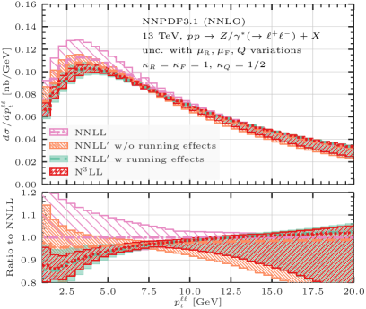
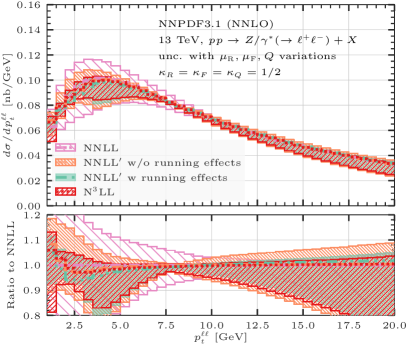
Figure 1: Resummed $p_{t}^{\ell\ell}$ spectrum in the inclusive setup at NNLL, NNLL^′, N³LL. Left panel: central scales $\kappa_{R}=\kappa_{F}=1$, $\kappa_{Q}=1/2$. Right panel: central scales $\kappa_{R}=\kappa_{F}=\kappa_{Q}=1/2$.

In Fig. 1 we show a comparison of pure resummed results for the di-lepton transverse-momentum $p_{t}^{\ell\ell}$ distribution in the inclusive setup at NNLL (pink), NNLL^′ without running-coupling effects (orange), NNLL^′ with running-coupling effects (green), and N³LL (red). The plot on the left panel displays variations around central scales $\kappa_{R}=\kappa_{F}=1$, $\kappa_{Q}=1/2$, while the right panel features central scales $\kappa_{R}=\kappa_{F}=\kappa_{Q}=1/2$. Both plots clearly show the benefits of the inclusion of ‘primed’ effects on the NNLL predictions at the level of central value and theoretical-uncertainty bands, especially in terms of shapes. We note that NNLL^′ predictions, both with and without running-coupling effects, are significantly closer to the full N³LL result than the NNLL one is, although the pattern of comparison somewhat depends on the chosen central-scale setup, with the running-coupling option closer to full N³LL on the left, and the opposite on the right panel. The uncertainty band of the NNLL^′ predictions is also significantly reduced below 10 GeV with respect to the NNLL one. The band relevant to the running-coupling option is smaller than the the non-running one, which is generally expected since the former encodes correct higher-order running-coupling information, absent in the latter. We note that across the entire $p_{t}^{\ell\ell}$ range the former band is also very similar to the N³LL one, and moreover, in all cases does it contain the central N³LL prediction, yielding a reliable estimate of the impact of missing higher-order terms. The difference between the two NNLL^′ results may become non negligible at very small $p_{t}^{\ell\ell}$ for certain scale setups (especially so when the central $\kappa_{Q}$ is different from the central $\kappa_{R}$, $\kappa_{F}$ values), which is also qualitatively expected as due to the approaching to a strong-coupling regime; in all cases the discrepancy is covered by the uncertainty band of the NNLL^′ with running-coupling option, which faithfully assesses the ambiguity related to the inclusion of beyond-accuracy running-coupling effects. In the following we choose the running-coupling option of ‘primed’ results as the default for our phenomenological study.

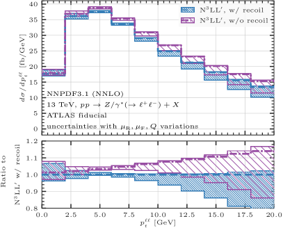
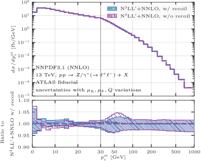
Figure 2: N³LL^′ (left) and N³LL^′ ​​+NNLO (right) $p_{t}^{\ell\ell}$ spectra in the fiducial ATLAS setup with (blue) and without (purple) recoil effects. In the right plot, the $x$ axis is linear up to 30 GeV and logarithmic above.

In Fig. 2 we assess the effect of the recoil prescription detailed in Sec. 3.4 on fiducial $p_{t}^{\ell\ell}$ predictions at N³LL^′ accuracy (where not explicitly stated, we employ the running-coupling option), both without (left panel) and with (right panel) additive matching (59) to the fixed NNLO differential result. The uncertainty band stems from variations around central scales $\kappa_{R}=\kappa_{F}=1$, $\kappa_{Q}=1/2$, while the matched result includes variation of $v_{0}$ as well. The inclusion of recoil (blue, as opposed to purple not featuring recoil effects) gives rise to an expected linear power correction in the pure resummed case, as can be specifically checked in the lower inset of the left panel. After matching to fixed order, recoil induces a marginal $\mp 1$% distortion of the spectrum below 20 GeV, which is the leftover effect after the ${\cal O}(\alpha_{s}^{3})$ cancellation taking place between resummation and its expansion in (59). The uncertainty bands are also very similar across the whole phase space.

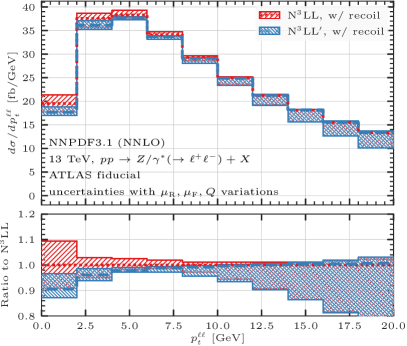
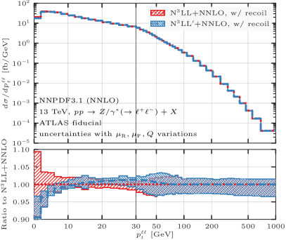
Figure 3: Left: resummed predictions at N³LL (red) and N³LL^′ (blue) for $p_{t}^{\ell\ell}$ in the fiducial ATLAS setup. Right: matched prediction at N³LL ​+NNLO (red) and N³LL^′ ​​+NNLO (blue). In the right plot, the $x$ axis is linear up to 30 GeV and logarithmic above.

Figure 3 displays a comparison, at the fiducial level and including recoil effects, between resummed results (left panel) at N³LL (red) and at N³LL^′ (blue) accuracy, and between matched results (right panel) at N³LL ​+NNLO (red) and at N³LL^′ ​​+NNLO (blue) accuracy. All variations are relevant to central-scale values $\kappa_{R}=\kappa_{F}=1$, $\kappa_{Q}=1/2$. The inclusion of ‘primed’ effects on the pure resummed prediction induces a distortion in the spectrum which is less than 2% above 5 GeV, and that can be as large as a few percent below, which is qualitatively consistent with (and quantitatively less pronounced than) what is shown for the NNLL^′ versus NNLL comparison in the left panel of Fig. 1, featuring the same central-scale setup. The uncertainty band undergoes a significant reduction below 10 GeV in passing from N³LL to N³LL^′ accuracy, by up to a factor of 2 towards $p_{t}^{\ell\ell}\to 0$. The matched results shown on the right panel largely inherit the features just described in the phase-space region dominated by resummation effects, whereas for $p_{t}^{\ell\ell}$ above 50 GeV the prediction is dominated by the fixed-order component, which is common to both. Overall, the N³LL^′ ​​+NNLO residual uncertainty band is at the level of 2 - 3% below 30 GeV (barring the first bin), and around 5% above 30 GeV.

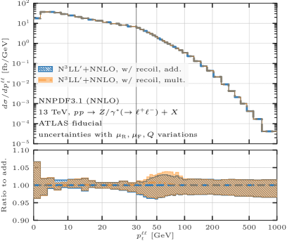
Figure 4: Comparison of additive (blue) and multiplicative (orange) matching prescriptions at N³LL^′ ​+NNLO, with recoil effects. The $x$ axis is linear up to 30 GeV and logarithmic above.

Fig. 4 shows a comparison of the default additive-matching prescription defined in eq. (59) (blue) with the multiplicative matching defined in eq. (61) (orange) at the N³LL^′ ​​+NNLO level, where both predictions include transverse-recoil effects. For reference, the central-scale setup is $\kappa_{R}=\kappa_{F}=1$, $\kappa_{Q}=1/2$, and the additive prediction is the same as in the right panel of Fig. 3. The theoretical systematics related to the choice of matching family results fairly negligible at this order, with the two predictions being essentially indistinguishable both at central scales, and with respect to uncertainty bands. As the envelope of the two different schemes essentially coincides with the single uncertainty bands, we refrain from adopting it as an estimate of matching systematics, and rather insist on the variation of parameter $v_{0}$ in a sensible range, such as [2/3, 3/2] around the central $v_{0}$ value, as better suited to this aim. This variation is responsible for the slight widening of the band between 30 GeV and 100 GeV, which we believe to reflect a genuine matching uncertainty in this region.

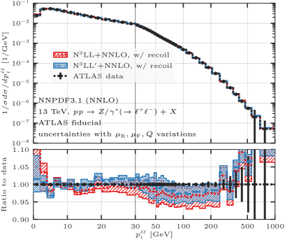
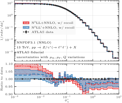
Figure 5: Comparison of matched predictions at N³LL ​+NNLO (red) and N³LL^′ +NNLO (blue) with ATLAS data Aad:2019wmn for $p_{t}^{\ell\ell}$ (left panel) and ${\phi^{*}_{\eta}}$ (right panel). The fixed-order component is turned off below ${\phi^{*}_{\eta}}=3.4\cdot 10^{-2}$ in the right panel, see main text for details. In the left plot, the $x$ axis is linear up to 30 GeV and logarithmic above.

In Fig. 5 we finally compare matched predictions in the fiducial setup to ATLAS data Aad:2019wmn , both for $p_{t}^{\ell\ell}$ (left panel) and for ${\phi^{*}_{\eta}}$ (right panel). The left panel includes the same theoretical predictions shown in the right panel of Fig. 3 (keeping the same colour code), which are here normalised to their cross section in order to match the convention of the shown data. The matched N³LL^′ ​​+NNLO predictions for $p_{t}^{\ell\ell}$ show a remarkable agreement with experimental data, with a theoretical-uncertainty band down to the 2 - 5% level, essentially overlapping with data in all bins form 0 to 200 GeV (barring one low-$p_{t}^{\ell\ell}$ bin, where the cancellation between the fixed-order and the expanded components is particularly delicate, and few middle-$p_{t}^{\ell\ell}$ bins where the agreement is only marginal). The inclusion of ‘primed’ effects tends to align the shape of the theoretical prediction to data, so that the former never departs more than 1 - 2% from the latter below 200 GeV, as opposed to the more visible relative distortion of the N³LL ​+NNLO below 5 GeV and above 50 GeV. The ${\phi^{*}_{\eta}}$ results on the right panel follow by and large the same pattern just seen for $p_{t}^{\ell\ell}$, with ‘primed’ effects being relevant to improve the data-theory agreement over the entire range, expecially at very small ${\phi^{*}_{\eta}}$, and theoretical uncertainties at or below the $\pm 3\%$ level.

We incidentally note that, due to the extremely soft and collinear regime probed by ${\phi^{*}_{\eta}}$ data, the fixed-order component features some fluctuations at small ${\phi^{*}_{\eta}}$; consequently, we have opted to turn it off in the first bins (up to ${\phi^{*}_{\eta}}=3.4\cdot 10^{-2}$), which implies that the matching formula in that region corresponds to the sole resummation output, multiplied by $Z(v)$. On the one hand this shows that resummation alone is capable of predicting data remarkably well both in shape and in normalisation at very small ${\phi^{*}_{\eta}}$; on the other hand it highlights the necessity of dedicated high-statistics fixed-order runs in order to reliably extract information on fiducial cross sections at N³LO by means of slicing techniques, especially in presence of symmetric lepton $p_{t}^{\ell^{\pm}}$ cuts.

5.2 Higgs results

For Higgs phenomenology we consider hadro-production at the 13 TeV LHC in an inclusive setup, with an un-decayed Higgs boson and no cuts, as well as in a fiducial setup, where we focus on the $H\to\gamma\gamma$ decay channel. We employ an effective-field-theoretical (HEFT) description of the gluon-fusion process where the the top quark running in the loops is integrated out, giving rise to an effective $ggH$ coupling. As seen above, the hard-function coefficients $H^{(2)}_{g}$ and $H^{(3)}_{g}$ encode the $m_{\rm top}$ dependence arising from the Wilson coefficient of the effective vertex. The fiducial volume is defined by the following set of cuts Aaboud:2018xdt

$$\min(p_{t}^{\gamma_{1}},p_{t}^{\gamma_{2}})>31.25~{}{\rm GeV}\,,\qquad\max(p_{t}^{\gamma_{1}},p_{t}^{\gamma_{2}})>43.75~{}{\rm GeV}\,,$$

$$0<|\eta^{\gamma_{1,2}}|<1.37\quad{\rm or}\quad 1.52<|\eta^{\gamma_{1,2}}|<2.37\,,\qquad|Y_{\gamma\gamma}|<2.37\,,$$ (64)

where $p_{t}^{\gamma_{i}}$ are the transverse momenta of the two photons, $\eta^{\gamma_{i}}$ are their pseudo-rapidities in the hadronic centre-of-mass frame, and $Y_{\gamma\gamma}$ is the photon-pair rapidity. In the definition of the fiducial phase-space cuts we do not include the photon-isolation requirement of Aaboud:2018xdt , since this would introduce additional non-global logarithmic corrections in the problem, spoiling the formal accuracy of the resummation. However, we point out that the photon-isolation is quite mild in this particular setup, hence it could faithfully be included at fixed order. The photon decay is predicted in the narrow-width approximation applying a branching ratio of $2.35\times 10^{-3}$.

For fiducial predictions we employ parton densities from the PDF4LHC15_nnlo_mc set Ball:2014uwa ; Butterworth:2015oua ; Dulat:2015mca ; Harland-Lang:2014zoa ; Carrazza:2015hva ; Watt:2012tq . Central renormalisation, factorisation, and resummation scales are set as $\mu_{R}=\kappa_{R}M_{H}$, $\mu_{F}=\kappa_{F}M_{H}$, $Q=\kappa_{Q}M_{H}$, respectively. Theoretical-uncertainty bands are obtained as explained in section 5.1 for the Drell-Yan case. In the inclusive setup, used solely to show the impact of running-coupling effects on ‘primed’ results, we employ the NNLO NNPDF3.1 PDF set Ball:2017nwa with $\alpha_{s}(M_{Z})=0.118$.

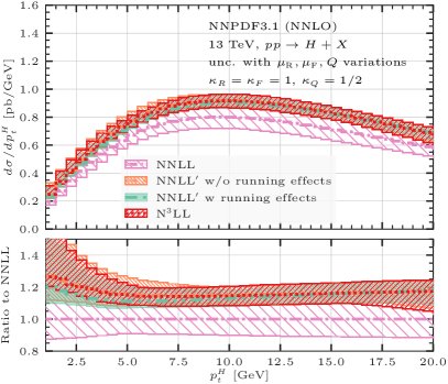
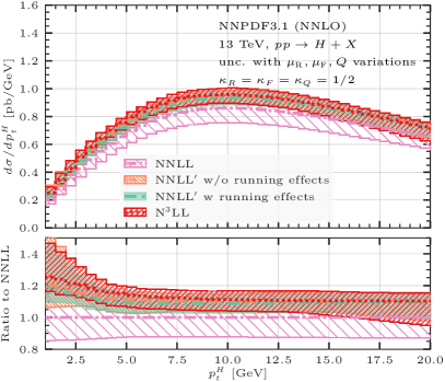
Figure 6: Resummed $p_{t}^{H}$ spectrum for inclusive Higgs production at NNLL, NNLL^′, N³LL. Left panel: central scales $\kappa_{R}=\kappa_{F}=1$, $\kappa_{Q}=1/2$. Right panel: central scales $\kappa_{R}=\kappa_{F}=\kappa_{Q}=1/2$.

In Fig. 6 we consider inclusive Higgs production, and show pure resummed predictions for the Higgs transverse momentum $p_{t}^{H}$ at NNLL, NNLL^′, and N³LL with central-scale choices $\kappa_{R}=\kappa_{F}=1$, $\kappa_{Q}=1/2$ (left panel), and $\kappa_{R}=\kappa_{F}=\kappa_{Q}=1/2$ (right panel). This figure, which is the exact analogue of Fig. 1 discussed above, aims at assessing the effect of including or not running-coupling effects in ‘primed’ results relevant for Higgs production. The benefit of including ‘primed’ predictions proves significant in this case as well, but with a different pattern with respect to Drell-Yan production. The shape distortion in passing from NNLL to NNLL^′ has a slightly more limited range, mainly extending up to 5 GeV in $p_{t}^{H}$; however, the normalisation of the theoretical curves is significantly affected, with ‘primed’ predictions correctly capturing the large $K$-factor, at the level of 15% at this perturbative order, which is known to arise in Higgs production. We note the the two different NNLL^′ predictions are fairly similar, and remarkably closer (in shape and normalisation) to the N³LL one than the bare NNLL is, both in terms of central value, and of uncertainty-band estimate. The central NNLL^′ prediction without running coupling tends to be slightly closer to the central N³LL one, while NNLL^′ with running coupling is slightly more similar to N³LL in terms of uncertainty band. In all cases does the central N³LL prediction lie well within the NNLL^′ running-coupling band, which we use as our default for the fiducial study.

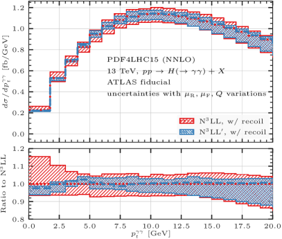
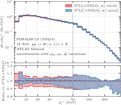
Figure 7: Left: resummed predictions at N³LL (red) and N³LL^′ (blue) for $p_{t}^{\gamma\gamma}$ in the fiducial ATLAS setup. Right: matched prediction at N³LL ​+NNLO (red) and N³LL^′ ​​+NNLO (blue). In the right plot, the $x$ axis is linear up to $p_{t}^{\gamma\gamma}=50$ GeV and logarithmic above.

Fig. 7 displays a comparison, relevant to the fiducial di-photon $p_{t}^{\gamma\gamma}$ spectrum, of N³LL^′ curves (blue) agains N³LL predictions (red), both without (left panel) and with (right panel) additive matching to NNLO. All predictions include recoil effects, so that this figure represents the Higgs-production analogue of Fig. 3, but referred to central scales $\kappa_{R}=\kappa_{F}=\kappa_{Q}=1/2$. The shape distortion with respect to N³LL predictions is more modest in the Higgs case with respect to Drell-Yan production, partly owing to the chosen central-scale setup; moreover, the induced $K$-factor is fairly close to unity at this order, which is sign of a good perturbative convergence. Overall, N³LL^′ predictions feature a significant reduction in theoretical uncertainty in comparison to N³LL ones, especially in the low-$p_{t}^{\gamma\gamma}$ region dominated by resummation. Residual uncertainty is as low as 5 - 7% below 10 GeV, and in the matched case it never exceeds 10% below 40 GeV.

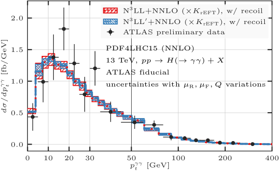
Figure 8: ATLAS data ATLAS-CONF-2019-029 against matched predictions at N³LL ​+NNLO (red) and N³LL^′ ​​+NNLO (blue) for the fiducial $p_{t}^{\gamma\gamma}$ spectrum. Theoretical predictions are rescaled by $K_{\rm rEFT}=1.06584$. The $x$ axis is linear up to $p_{t}^{\gamma\gamma}=50$ GeV and logarithmic above.

Finally, in Figure 8 we show a comparison of theoretical predictions for the fiducial $p_{t}^{\gamma\gamma}$ spectrum at N³LL ​+NNLO (red) and N³LL^′ ​​+NNLO (blue) level, with recoil effects, against ATLAS preliminary data ATLAS-CONF-2019-029 . Theoretical predictions, based on central scales $\kappa_{R}=\kappa_{F}=\kappa_{Q}=1/2$, have been rescaled by a factor $K_{\rm rEFT}=1.06584$ to account for the exact top-quark mass dependence at LO.

6 Conclusion

In this article we have presented state-of-the-art differential predictions relevant for colour-singlet hadro-production at the LHC within the RadISH framework, up to N³LL^′ ​​+NNLO order. Such a level of accuracy in the resummed component is reached by supplementing the previously available N³LL result with the complete set of constant terms of relative order ${\cal O}(\alpha_{s}^{3})$ with respect to the Born level. We have documented in detail how the inclusion of such terms is achieved in RadISH, as well as the validation we have performed to confirm the correctness of their numerical implementation. In this article we have focused on neutral Drell-Yan and Higgs production, although we stress that the formalism used here can be straightforwardly applied to the charged Drell-Yan case as well.

We have assessed the behaviour of ‘primed’ predictions in inclusive Drell-Yan and Higgs production in a comparison of two different NNLL^′ prescriptions (including or not higher-order running-coupling effects, respectively) with N³LL. This has given us confidence on the mutual consistency of the two ‘primed’ results, and on the reliability of their quoted uncertainty bands, in view of comparing results based on N³LL^′ predictions with experimental data. In particular, in all considered cases are the NNLL^′ uncertainty bands capable of encompassing the N³LL central prediction, and to correctly estimate the higher-order running-coupling ambiguity underlying the definition of ‘primed’ accuracy.

The results presented here are fully exclusive with respect to the Born phase-space variables, lending themselves to be flexibly adapted to the fiducial volumes considered in realistic experimental analyses. In order to more accurately simulate the kinematics of the colour-singlet decay products (we considered a lepton pair in the case of Drell-Yan production, and a photon pair in the case of Higgs production), we have consistently encoded in our prediction a prescription for the treatment of the singlet’s transverse recoil against soft and collinear QCD initial-state radiation. This includes in our results the full set of linear next-to-leading-power corrections for azimuthally symmetric observables, such as the transverse momentum of the singlet.

The inclusion of transverse-recoil effects, which is performed at the level of differential (as opposed to cumulative) cross sections, and the availability of ${\cal O}(\alpha_{s}^{3})$ constant terms in the resummed component, has led to the definition of two differential matching prescriptions, belonging to the additive and multiplicative families, respectively. We have compared the two schemes in Drell-Yan production, and found very good agreement between them, showing that matching systematics are well under control. Variation of matching parameters has anyway been conservatively included in the estimate of the theoretical uncertainties.

Although the ingredients presented above would immediately allow us to quote numbers for the N³LO fiducial Drell-Yan and Higgs cross sections, we refrain from doing so in the present article, as in our opinion such a high-precision prediction requires dedicated high-statistics fixed-order runs in order to avoid potential numerical biases. This is especially the case in the context of a slicing technique in presence of symmetric cuts on the transverse momentum of the singlet’s decay products. We leave this development for future work.

As a general upshot of the present work, which we have documented both in Drell-Yan and in Higgs production, the inclusion of ‘primed’ effects is highly beneficial for the stability of the theoretical prediction, leading to a significant reduction in the residual theoretical uncertainty. In the case of our highest-accuracy result, N³LL^′ ​​+NNLO, such a reduction can be as large as a factor of 2 in the region dominated by resummation.

For the di-lepton $p_{t}^{\ell\ell}$ spectrum in Drell-Yan production, the N³LL^′ ​​+NNLO prediction is shown to improve the comparison to ATLAS data with respect to N³LL ​+NNLO. The theory-data agreement is now at a remarkable level of 1 - 2% below 200 GeV, and the residual theory uncertainty is at or below the 2 - 5% level in that phase-space region. Same considerations hold for the ${\phi^{*}_{\eta}}$ observable, with the N³LL^′ ​​+NNLO band nicely overlapping with data over the entire range, with leftover uncertainty below $\pm 3\%$. For Higgs production we find a similar qualitative pattern, with N³LL^′ predictions featuring an uncertainty at the level of 5% at very low di-photon $p_{t}^{\gamma\gamma}$, and matched N³LL^′ ​​+NNLO results well below $\pm 10\%$ accuracy over the entire $p_{t}^{\gamma\gamma}$ range.

The RadISH code used for the predictions shown in this paper will be made public in due time, and the results are available from the authors upon request.

Appendix A Parton luminosities up to N³LL^′

We report the explicit expression for the parton luminosities employed in the main text, up to N³LL^′ accuracy. By defining the coupling factors

$$\bar{\alpha}_{s(0)} = \alpha_{s}(\mu_{R})\,,\qquad\bar{\alpha}_{s(1)}\,=\,\frac{\alpha_{s}(\mu_{R})}{\xi}\,,\qquad\bar{\alpha}_{s(2)}\,=\,\frac{\alpha_{s}(\mu_{R})}{\xi}\bigg{[}1-\alpha_{s}(\mu_{R})\,\frac{\beta_{1}}{\beta_{0}}\,\frac{\ln\xi}{\xi}\bigg{]}\,,$$

$$\bar{\alpha}_{s(3)} = \frac{\alpha_{s}(\mu_{R})}{\xi}\bigg{[}1-\alpha_{s}(\mu_{R})\,\frac{\beta_{1}}{\beta_{0}}\,\frac{\ln\xi}{\xi}+\,\alpha_{s}^{2}(\mu_{R})\,\frac{\beta_{1}^{2}}{\beta_{0}^{2}}\,\frac{\ln^{2}\xi-\ln\xi-(1-\xi)(1-\beta_{0}\beta_{2}/\beta_{1}^{2})}{\xi^{2}}\bigg{]}\,,$$ (65)

with $\xi=1-2\alpha_{s}(\mu_{R})\beta_{0}\ln(\mu_{R}/k_{t1})$, which correspond to $\alpha_{s}(k_{t1})$ written in terms of $\alpha_{s}(\mu_{R})$ at 0, 1, 2, 3 loops, and

$$\beta_{0} = \frac{11C_{A}-2n_{f}}{12\pi}\,,\qquad\beta_{1}\,=\,\frac{17C_{A}^{2}-5C_{A}n_{f}-3C_{F}n_{f}}{24\pi^{2}}\,,$$

$$\beta_{2} = \frac{2857C_{A}^{3}+(54C_{F}^{2}-615C_{F}C_{A}-1415C_{A}^{2})n_{f}+(66C_{F}+79C_{A})n_{f}^{2}}{3456\pi^{3}}\,,$$ (66)

the standard luminosities can be compactly written as

$${\cal L}_{\rm NLL}(k_{t1}) = \sum_{c,c^{\prime}}\frac{{\rm d}|{\cal M}_{B}|_{cc^{\prime}}^{2}}{{\rm d}\Phi_{B}}\,f_{c}(k_{t1},x_{1})\,f_{c^{\prime}}(k_{t1},x_{2})\,,$$ (67)

$${\cal L}_{\rm NNLL}(k_{t1}) = \sum_{c,c^{\prime}}\frac{{\rm d}|{\cal M}_{B}|_{cc^{\prime}}^{2}}{{\rm d}\Phi_{B}}\,\sum_{i,j}\int_{x_{1}}^{1}\frac{{\rm d}z_{1}}{z_{1}}\int_{x_{2}}^{1}\frac{{\rm d}z_{2}}{z_{2}}\,f_{i}\Big{(}k_{t1},\frac{x_{1}}{z_{1}}\Big{)}\,f_{j}\Big{(}k_{t1},\frac{x_{2}}{z_{2}}\Big{)}$$ (68)

$$\times\,\Bigg{\{}\delta_{ci}\,\delta_{c^{\prime}j}\,\delta(1-z_{1})\,\delta(1-z_{2})\sum_{k=0}^{1}\Big{(}\frac{\bar{\alpha}_{s(0)}}{2\pi}\Big{)}^{k}H^{(k)}(\mu_{R})$$

$$\quad+\,\frac{\bar{\alpha}_{s(1)}}{2\pi}\Big{(}C_{ci}^{(1)}(z_{1})\delta(1-z_{2})\delta_{c^{\prime}j}+\,\{z_{1},c,i\,\leftrightarrow\,z_{2},c^{\prime},j\}\Big{)}\Bigg{\}}\,,$$

$${\cal L}_{\rm N^{3}LL}(k_{t1}) = \sum_{c,c^{\prime}}\frac{{\rm d}|{\cal M}_{B}|_{cc^{\prime}}^{2}}{{\rm d}\Phi_{B}}\,\sum_{i,j}\int_{x_{1}}^{1}\frac{{\rm d}z_{1}}{z_{1}}\int_{x_{2}}^{1}\frac{{\rm d}z_{2}}{z_{2}}\,f_{i}\Big{(}k_{t1},\frac{x_{1}}{z_{1}}\Big{)}\,f_{j}\Big{(}k_{t1},\frac{x_{2}}{z_{2}}\Big{)}$$ (69)

$$\times\,\Bigg{\{}\delta_{ci}\,\delta_{c^{\prime}j}\,\delta(1-z_{1})\,\delta(1-z_{2})\sum_{k=0}^{2}\Big{(}\frac{\bar{\alpha}_{s(0)}}{2\pi}\Big{)}^{k}H^{(k)}(\mu_{R})$$

$$\quad+\,\frac{\bar{\alpha}_{s(2)}}{2\pi}\Big{(}C_{ci}^{(1)}(z_{1})\,\delta(1-z_{2})\,\delta_{c^{\prime}j}+\,\{z_{1},c,i\,\leftrightarrow\,z_{2},c^{\prime},j\}\Big{)}$$

$$\quad+\,\Big{(}\frac{\bar{\alpha}_{s(1)}}{2\pi}\Big{)}^{2}\Big{(}C_{ci}^{(2)}(z_{1})\,\delta(1-z_{2})\,\delta_{c^{\prime}j}+\{z_{1},c,i\,\leftrightarrow\,z_{2},c^{\prime},j\}$$

$$\hskip 56.9055pt+\,C_{ci}^{(1)}(z_{1})\,C_{c^{\prime}j}^{(1)}(z_{2})+G_{ci}^{(1)}(z_{1})\,G_{c^{\prime}j}^{(1)}(z_{2})\Big{)}$$

$$\quad+\,\frac{\bar{\alpha}_{s(0)}\bar{\alpha}_{s(1)}}{(2\pi)^{2}}H^{(1)}(\mu_{R})\Big{(}C_{ci}^{(1)}(z_{1})\,\delta(1-z_{2})\,\delta_{c^{\prime}j}+\{z_{1},c,i\,\leftrightarrow\,z_{2},c^{\prime},j\}\Big{)}\Bigg{\}}\,,$$

$${\cal L}_{\rm N^{4}LL}(k_{t1}) = \sum_{c,c^{\prime}}\frac{{\rm d}|{\cal M}_{B}|_{cc^{\prime}}^{2}}{{\rm d}\Phi_{B}}\,\sum_{i,j}\int_{x_{1}}^{1}\frac{{\rm d}z_{1}}{z_{1}}\int_{x_{2}}^{1}\frac{{\rm d}z_{2}}{z_{2}}\,f_{i}\Big{(}k_{t1},\frac{x_{1}}{z_{1}}\Big{)}\,f_{j}\Big{(}k_{t1},\frac{x_{2}}{z_{2}}\Big{)}$$ (70)

$$\times\,\Bigg{\{}\delta_{ci}\,\delta_{c^{\prime}j}\,\delta(1-z_{1})\,\delta(1-z_{2})\sum_{k=0}^{3}\Big{(}\frac{\bar{\alpha}_{s(0)}}{2\pi}\Big{)}^{k}H^{(k)}(\mu_{R})$$

$$\quad+\,\frac{\bar{\alpha}_{s(3)}}{2\pi}\Big{(}C_{ci}^{(1)}(z_{1})\,\delta(1-z_{2})\,\delta_{c^{\prime}j}+\,\{z_{1},c,i\,\leftrightarrow\,z_{2},c^{\prime},j\}\Big{)}$$

$$\quad+\,\Big{(}\frac{\bar{\alpha}_{s(2)}}{2\pi}\Big{)}^{2}\Big{(}C_{ci}^{(2)}(z_{1})\,\delta(1-z_{2})\,\delta_{c^{\prime}j}+\{z_{1},c,i\,\leftrightarrow\,z_{2},c^{\prime},j\}$$

$$\hskip 56.9055pt+\,C_{ci}^{(1)}(z_{1})\,C_{c^{\prime}j}^{(1)}(z_{2})+G_{ci}^{(1)}(z_{1})\,G_{c^{\prime}j}^{(1)}(z_{2})\Big{)}$$

$$\quad+\,\frac{\bar{\alpha}_{s(0)}\bar{\alpha}_{s(2)}}{(2\pi)^{2}}H^{(1)}(\mu_{R})\Big{(}C_{ci}^{(1)}(z_{1})\,\delta(1-z_{2})\,\delta_{c^{\prime}j}+\{z_{1},c,i\,\leftrightarrow\,z_{2},c^{\prime},j\}\Big{)}$$

$$\quad+\,\Big{(}\frac{\bar{\alpha}_{s(1)}}{2\pi}\Big{)}^{3}\Big{(}C_{ci}^{(3)}(z_{1})\,\delta(1-z_{2})\,\delta_{c^{\prime}j}+C_{ci}^{(2)}(z_{1})\,C_{c^{\prime}j}^{(1)}(z_{2})$$

$$\hskip 56.9055pt+\,G_{ci}^{(2)}(z_{1})\,G_{c^{\prime}j}^{(1)}(z_{2})+\{z_{1},c,i\,\leftrightarrow\,z_{2},c^{\prime},j\}\Big{)}$$

$$\quad+\,\frac{\bar{\alpha}_{s(0)}\bar{\alpha}_{s(1)}^{2}}{(2\pi)^{3}}H^{(1)}(\mu_{R})\Big{(}C_{ci}^{(2)}(z_{1})\,\delta(1-z_{2})\,\delta_{c^{\prime}j}+\{z_{1},c,i\,\leftrightarrow\,z_{2},c^{\prime},j\}$$

$$\hskip 56.9055pt+\,C_{ci}^{(1)}(z_{1})\,C_{c^{\prime}j}^{(1)}(z_{2})+G_{ci}^{(1)}(z_{1})\,G_{c^{\prime}j}^{(1)}(z_{2})\Big{)}$$

$$\quad+\,\frac{\bar{\alpha}^{2}_{s(0)}\bar{\alpha}_{s(1)}}{(2\pi)^{3}}H^{(2)}(\mu_{R})\Big{(}C_{ci}^{(1)}(z_{1})\,\delta(1-z_{2})\,\delta_{c^{\prime}j}+\{z_{1},c,i\,\leftrightarrow\,z_{2},c^{\prime},j\}\Big{)}\Bigg{\}}\,,$$

where $H^{(0)}(\mu_{R})=1$, $x_{1,2}={\rm e}^{\pm Y}M/\sqrt{s}$, and $Y$ is the Born-level rapidity of the colour singlet in the centre-of-mass frame of the collision, with energy $\sqrt{s}$.

As for the luminosities relevant for ‘primed’ predictions, they assume a different functional form for the running or non-running options, described in the main text. In the running case, we just set ${\cal L}_{{\rm N}^{k}{\rm LL}^{\prime}}={\cal L}_{{\rm N}^{k+1}{\rm LL}}$; in the non-running case, ${\cal L}_{{\rm N}^{k}{\rm LL}^{\prime}}=\hat{\cal L}_{{\rm N}^{k+1}{\rm LL}}$, where the $\hat{\cal L}_{{\rm N}^{k+1}{\rm LL}}$ corresponds to a luminosity ${\cal L}_{{\rm N}^{k+1}{\rm LL}}$ with the replacement $\bar{\alpha}_{s(j)}\to\bar{\alpha}_{s(j-1)}$ for $j>0$.

Appendix B V-A structure of the form factor in the neutral Drell-Yan process

In this subsection we discuss the subtleties arising in the extraction of the hard-virtual corrections to the form factor for the neutral-current Drell-Yan process

$$q(p_{1})\ \bar{q}(p_{2})\,\to\,Z/\gamma^{*}\,\to\,\ell^{-}(p_{3})\ \ell^{+}(p_{4})\,,$$ (71)

that we will denote with the shortcut $Z/\gamma^{*}$, although in the following the dependence upon the final-state leptonic momenta is explicitly taken into account.

Before discussing how the hard-virtual coefficients in eq. (3.1) are extracted from the loop corrections to the form factor, it is useful to recall the structure of the Drell-Yan tree-level amplitude expressed in terms of spinor currents. The fermion-antifermion-photon, and fermion-antifermion-$Z$ vertices are defined as

$$-i|e|Q_{f}\gamma^{\mu}\,,\hskip 28.45274pt-i|e|(V_{f}+A_{f}\gamma_{5})\gamma^{\mu}\,,$$ (72)

respectively, where $Q_{f}$ is the charge of the fermion in units of the positron charge $|e|$, and

$$V_{f}\,=\,\frac{T^{3}_{f}-2Q_{f}\sin^{2}\theta_{W}}{2\sin\theta_{W}\cos\theta_{W}}\,,\qquad A_{f}\,=\,\frac{T^{3}_{f}}{2\sin\theta_{W}\cos\theta_{W}}\,,$$ (73)

$\theta_{W}$ being the weak mixing angle and $T^{3}_{f}=\pm 1/2$ the weak isospin quantum number of the fermion type $f$. The fermionic currents relevant for the process in eq. (71) are

$$J_{V;A}^{\mu(0)}(f)\,=\,\bar{F}\ [1;\gamma_{5}]\gamma^{\mu}F\,,$$ (74)

where, for the initial-state quark current ($f=q$), the Dirac spinors read $\bar{F}=\bar{v}(p_{2})$ and ${F}=u(p_{1})$, whereas, for the leptonic current ($f=\ell$), $\bar{F}=\bar{u}(p_{3})$ and ${F}=v(p_{4})$.

The tree-level amplitude can be written as

$$\mathcal{M}^{(0)} = \frac{1}{q^{2}}(Q_{q}J^{(0)}_{V}(q))\cdot(Q_{\ell}J^{(0)}_{V}(\ell))$$ (75)

$$+\,\frac{1}{(q^{2}-M_{Z}^{2})+iM_{Z}\Gamma_{Z}}\Big{(}V_{q}J^{(0)}_{V}(q)+A_{q}J^{(0)}_{A}(q)\Big{)}\cdot\Big{(}V_{\ell}J^{(0)}_{V}(\ell)+A_{\ell}J^{(0)}_{A}(\ell)\Big{)}\,,$$

where $q=p_{1}+p_{2}$, and the symbol ‘$\cdot$’ represents the Lorentz dot product (among currents, in this case). The superscript on the currents indicates the loop order at which they are computed. By denoting the products of currents of fermion line $f$ with

$$[JJ^{(ij)}_{XY}(f)]^{\bar{\mu}\mu}\,=\,[J^{\bar{\mu}(i)}_{X}(f)]^{{\dagger}}\,[J^{\mu(j)}_{Y}(f)]\,,\qquad XY\,\in\,\left\{VV,\,AA,\,AV,\,VA\right\}\,,$$ (76)

the tree-level squared amplitude reads (up to global factors not relevant for the present discussion)

$$|\mathcal{M}^{(0)}|^{2}\,\propto\,|A_{\gamma}|^{2}+|A_{Z}|^{2}+2\Re(A_{\gamma}^{*}\,A_{Z})\,,$$ (77)

where

$$|A_{\gamma}|^{2}\,=\,\frac{1}{q^{4}}\ Q_{q}^{2}Q_{\ell}^{2}\ [JJ^{(00)}_{VV}(q)]^{\bar{\mu}\mu}[JJ^{(00)}_{VV}(\ell)]_{\bar{\mu}\mu}\,,$$

$$|A_{Z}|^{2}\,=\,\frac{1}{(q^{2}-M_{Z}^{2})^{2}+(M_{Z}\Gamma_{Z})^{2}}$$

$$\hskip 56.9055pt\left[V_{q}^{2}[JJ^{(00)}_{VV}(q)]+A_{q}^{2}[JJ^{(00)}_{AA}(q)]+A_{q}V_{q}\Big{(}[JJ^{(00)}_{VA}(q)]+[JJ^{(00)}_{AV}(q)]\Big{)}\right]^{\bar{\mu}\mu}$$

$$\hskip 56.9055pt\left[V_{\ell}^{2}[JJ^{(00)}_{VV}(\ell)]+A_{\ell}^{2}[JJ^{(00)}_{AA}(\ell)]+A_{\ell}V_{\ell}\Big{(}[JJ^{(00)}_{VA}(\ell)]+[JJ^{(00)}_{AV}(\ell)]\Big{)}\right]_{\bar{\mu}\mu}$$

$$\phantom{|A_{Z}|^{2}}\,=\,\frac{1}{(q^{2}-M_{Z}^{2})^{2}+(M_{Z}\Gamma_{Z})^{2}}\Big{\{}\left(V_{q}^{2}+A_{q}^{2}\right)\left(V_{\ell}^{2}+A_{\ell}^{2}\right)[JJ^{(00)}_{VV}(q)]^{\bar{\mu}\mu}[JJ^{(00)}_{VV}(\ell)]_{\bar{\mu}\mu}$$

$$\hskip 150.79968pt+\,4A_{q}V_{q}A_{\ell}V_{\ell}\,[JJ^{(00)}_{VA}(q)]^{\bar{\mu}\mu}[JJ^{(00)}_{VA}(\ell)]_{\bar{\mu}\mu}\Big{\}}\,,$$

$$2\Re(A_{\gamma}^{*}\,A_{Z})\,=\,\frac{2(q^{2}-M_{Z}^{2})}{q^{2}[(q^{2}-M_{Z}^{2})^{2}+(M_{Z}\Gamma_{Z})^{2}]}\ \Big{[}Q_{q}V_{q}[JJ^{(00)}_{VV}(q)]+Q_{q}A_{q}[JJ^{(00)}_{VA}(q)]\Big{]}^{\bar{\mu}\mu}$$

$$\hskip 179.25244pt\Big{[}Q_{\ell}V_{\ell}[JJ^{(00)}_{VV}(\ell)]+Q_{\ell}A_{\ell}[JJ^{(00)}_{VA}(\ell)]\Big{]}_{\bar{\mu}\mu}$$

$$\phantom{2\Re(A_{\gamma}^{*}A_{Z})}=\frac{2(q^{2}-M_{Z}^{2})}{q^{2}[(q^{2}-M_{Z}^{2})^{2}+(M_{Z}\Gamma_{Z})^{2}]}\Big{\{}Q_{q}V_{q}Q_{\ell}V_{\ell}[JJ^{(00)}_{VV}(q)]^{\bar{\mu}\mu}[JJ^{(00)}_{VV}(\ell)]_{\bar{\mu}\mu}$$

$$\hskip 179.25244pt+\,Q_{q}A_{q}Q_{\ell}A_{\ell}[JJ^{(00)}_{VA}(q)]^{\bar{\mu}\mu}[JJ^{(00)}_{VA}(\ell)]_{\bar{\mu}\mu}\Big{\}}\,.$$ (78)

The $H^{(n)}(\mu_{R})$ coefficients in eq. (3.1) are of pure hard-virtual origin, and they are obtained from the finite parts of the $\rm\overline{MS}$-renormalised loop corrections (‘r,f’ in the equations below) to the tree-level amplitude. For $Z/\gamma^{*}$ production, if one solely considers loop diagrams where the external quark line is directly connected to the $Z/\gamma^{*}$ vertex, the full tree-level squared amplitude (77) can be factored in front of the hard function, namely up to three loops one has

$$\Big{|}\sum_{n=0}^{3}\left(\frac{\alpha_{s}}{2\pi}\right)^{n}\,\mathcal{M}^{(n)}\Big{|}^{2}_{\text{r,f}}=|\mathcal{M}^{(0)}|^{2}\,\sum_{n=0}^{3}\left(\frac{\alpha_{s}}{2\pi}\right)^{n}\,H^{(n)}+{\cal O}(\alpha_{s}^{4})\,,$$ (79)

where $\mathcal{M}^{(n)}$ has the same structure as the one given in (75), but it includes the ${\cal O}(\alpha_{s}^{n})$ vertex corrections to the fermionic currents $J_{V;A}^{\mu}(q)$,

$$J_{V;A}^{\mu}(q)\,=\,\sum_{n=0}^{3}\left(\frac{\alpha_{s}}{2\pi}\right)^{n}J^{(n)}_{V;A}(q)\,.$$ (80)

To convince oneself that this is indeed the case, one can consider the first-order coefficient $H^{(1)}$ of the hard-virtual function, that is given by $\{2\Re({\mathcal{M}^{(0)}}^{*}\mathcal{M}^{(1)})\}_{\text{r,f}}$. Within this contribution, the hadronic tensor features Dirac traces involving the product of two quark vector currents $[JJ^{(01)}_{VV}(q)]$, of two quark axial-vector currents $[JJ^{(01)}_{AA}(q)]$, and mixed terms, such as $[JJ^{(01)}_{VA}(q)]$. The radiative corrections to these three current correlators are the same, and they can be extracted from the quark form factor, despite the latter quantity is defined as the coupling of a virtual photon to a massless quark-antiquark pair, and hence, by definition, it contains the radiative corrections to $J_{V}^{\mu}(q)$, i.e. to the vector form factor. The physical reason why the radiative corrections to the massless vector and axial-vector form factor are the same ultimately stems from chirality conservation in QCD. Algorithmically, this a consequence of the properties of the $\gamma_{5}$ matrix: the Dirac trace in $[JJ^{(01)}_{AA}(q)]$ gives the same result as the one in $[JJ^{(01)}_{VV}(q)]$, therefore the $A_{q}^{2}$ term receives exactly the same radiative corrections of, e.g., the term $Q_{q}^{2}$ Hamberg:1990np . The computation of the radiative corrections to the terms proportional to $V_{q}A_{q}$ and $Q_{q}A_{q}$ is more delicate, as they involve a fermionic trace with just one $\gamma_{5}$ matrix, hence they require a consistent treatment of the axial-vector current in $d$ dimensions, which requires care from two loops Melnikov:2006kv ; Larin:1993tq . Eventually, as happens at tree level, the only non-vanishing contraction of $[JJ^{(01)}_{VA}(q)]$ is with $[JJ^{(00)}_{VA}(\ell)]$, yielding terms proportional to $V_{q}A_{q}V_{\ell}A_{\ell}$ (and $Q_{q}A_{q}Q_{\ell}A_{\ell}$) and with exactly the same radiative correction as the term $[JJ^{(01)}_{VV}(q)]$ $[JJ^{(00)}_{VV}(\ell)]$. The same property holds also at two and three loops.

In the light of the above discussion, for $Z/\gamma^{*}$ production, the tree-level squared amplitude (77) can be factored out, as in eq. (79), and the $H^{(n)}$ coefficient can be obtained from the quark form factor at $n$ loops.

Starting from NNLO, the vertex corrections to $Z/\gamma^{*}$ production contain graphs where the external off-shell gauge boson does not couple directly to the external quark line with flavour $f=q$, but rather to an internal closed fermion loop.

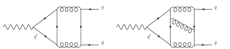
Figure 9: Example of Feynman diagrams contributing to the ‘singlet’ contribution at two and three loops.

In Fig. 9 we show representative diagrams at two and three loops. For such terms, customarily referred to as ‘singlet’ contributions, the factorisation in (79) is violated. Up to N³LO, $Z/\gamma^{*}$ production features two singlet contributions, namely

• non-vanishing finite corrections entering the axial-vector current but not the vector one, starting from two loops;

• corrections to the vector and axial-vector currents not factorising the tree-level form factor, at three loops.

As for contribution (a), at two loops the singlet correction to the vector current vanishes identically for each quark running in the fermion loop, by means of Furry’s theorem. Since the axial-vector coupling is proportional to $T^{3}_{f}$, within a given generation, the singlet correction to the latter also vanishes, provided the two quarks are degenerate in mass. Such a cancellation does not take place exactly in the third family. The leftover contribution, finite owing to the fact that the Standard Model is anomaly free, and vanishing in the $m_{\rm top}\to m_{\rm bottom}$ limit, has been computed in ref. Dicus:1985wx . For a given external quark line $q$, the radiative correction is proportional to $A_{q}\sum_{q^{\prime}}A_{q^{\prime}}J(m_{q^{\prime}},M_{Z})$ (eq. (7), Ref. Dicus:1985wx ). As this is a correction to $H^{(2)}$ that is proportional to $[JJ^{(00)}_{AA}(q)]$ but whose coupling is not proportional to $A_{q}^{2}$, it does not factorise $|\mathcal{M}^{(0)}|^{2}$. To our knowledge, these contributions are typically not included in resummed calculations. In our implementation, we have not included these axial corrections to the vertex.

We also stress that at ${\cal O}(\alpha_{s}^{2})$ there are other terms of this type arising from the ‘real-virtual’ interference of the $\ell^{+}\ell^{-}$+1 jet matrix elements. Similarly to the two-loop singlet axial corrections to the vertex, these terms are UV- and IR-finite, and vanish for each mass-degenerate quark family running in the fermion loop. Such ‘real-virtual’ corrections are also absent from our prediction.

The singlet contribution (b) to the quark form factor at three-loops has been computed in Refs. Baikov:2009bg ; Lee:2010cga ; Gehrmann:2010ue . In our notation, it contributes to the third-order expansion of $J^{\mu}_{V}(q)$ as

$$\left(\frac{\alpha_{s}}{2\pi}\right)^{3}J^{(3)}_{V}(q)\,\,\ni\,\,\left(\frac{\alpha_{s}}{2\pi}\right)^{3}J^{(3s)}_{V}(q)\,\,\equiv\,\,\left(\frac{\alpha_{s}}{2\pi}\right)^{3}C_{3}^{s}\,J_{V}(q)\,,$$ (81)

where

$$C_{3}^{s} = C_{F}\frac{N_{c}^{2}-4}{8N_{c}}\,\left(4-\frac{80}{3}\zeta_{5}+\frac{14}{3}\zeta_{3}+10\zeta_{2}-\frac{2}{5}\zeta_{2}^{2}\right)\,.$$ (82)

The $J^{(3s)}_{V}(q)$ current couples to the external quark line in the loop amplitude through $\sum_{q^{\prime}}Q_{q^{\prime}}$ (or $\sum_{q^{\prime}}V_{q^{\prime}}$) for $\gamma^{*}$ (or $Z$) exchange, where index $q^{\prime}$ labels all possible quark flavours running in the closed fermion loop. The singlet contribution enters the hard-virtual coefficient through the interference term $2\Re({\mathcal{M}^{(0)}}^{*}\mathcal{M}^{(3s)})$ (we drop the subscript r,f as $J^{(3s)}_{V}(q)$ is UV- and IR-finite), where

$$\mathcal{M}^{(3s)} = \frac{\sum_{q^{\prime}}Q_{q^{\prime}}Q_{\ell}}{q^{2}}J^{(3s)}_{V}(q)\cdot J_{V}(\ell)+$$ (83)

$$+\,\frac{\sum_{q^{\prime}}V_{q^{\prime}}}{(q^{2}-M_{Z}^{2})+iM_{Z}\Gamma_{Z}}J^{(3s)}_{V}(q)\cdot\Big{(}V_{\ell}J_{V}(\ell)+A_{\ell}J_{A}(\ell)\Big{)}\,.$$

We note that, in case of $\gamma^{*}$ production alone, one could collect a term $\sum_{q^{\prime}}Q_{q^{\prime}}/Q_{q}$ in the first line of eq. (83), thereby expressing the full result in a factorised form, as done in refs. Baikov:2009bg ; Lee:2010cga ; Gehrmann:2010ue , which is not possible when considering both $\gamma^{*}$ and $Z$ channels.

By taking the interference with the tree-level amplitude (75), one gets

$$2\Re({\mathcal{M}^{(0)}}^{*}\mathcal{M}^{(3s)})\,=\,2\left\{|A^{(03s)}_{\gamma}|^{2}+|A^{(03s)}_{Z}|^{2}+I^{(03s)}_{\gamma^{*}/Z}\right\}\,,$$ (84)

where

$$|A^{(03s)}_{\gamma}|^{2} = \frac{C_{3}^{s}\sum_{q^{\prime}}Q_{q^{\prime}}}{q^{4}}\ Q_{q}Q_{\ell}^{2}\ [JJ^{(00)}_{VV}(q)]^{\bar{\mu}\mu}[JJ^{(00)}_{VV}(\ell)]_{\bar{\mu}\mu}\,,$$ (85)

$$|A^{(03s)}_{Z}|^{2} = \frac{C_{3}^{s}\sum_{q^{\prime}}V_{q^{\prime}}}{(q^{2}-M_{Z}^{2})^{2}+M_{Z}^{2}\Gamma_{Z}^{2}}\,\Big{\{}V_{q}\left(V_{\ell}^{2}+A_{\ell}^{2}\right)[JJ^{(00)}_{VV}(q)]^{\bar{\mu}\mu}\,[JJ^{(00)}_{VV}(\ell)]_{\bar{\mu}\mu}$$

$$\hskip 99.58464pt+\,2A_{q}A_{\ell}V_{\ell}\,[JJ^{(00)}_{VA}(q)]^{\bar{\mu}\mu}\,[JJ^{(00)}_{VA}(\ell)]_{\bar{\mu}\mu}\Big{\}}\,,$$

$$I^{(03s)}_{\gamma^{*}/Z} = \frac{C_{3}^{s}(q^{2}-M_{Z}^{2})}{q^{2}[(q^{2}-M_{Z}^{2})^{2}+M_{Z}^{2}\Gamma_{Z}^{2}]}\ \Big{\{}Q_{\ell}V_{\ell}\Big{(}Q_{q}\sum_{q^{\prime}}V_{q^{\prime}}+V_{q}\sum_{q^{\prime}}Q_{q^{\prime}}\Big{)}[JJ^{(00)}_{VV}(q)]^{\bar{\mu}\mu}[JJ^{(00)}_{VV}(\ell)]_{\bar{\mu}\mu}$$ (86)

$$\hskip 99.58464pt+\,Q_{\ell}A_{q}A_{\ell}\sum_{q^{\prime}}Q_{q^{\prime}}\,[JJ^{(00)}_{VA}(q)]^{\bar{\mu}\mu}[JJ^{(00)}_{VA}(\ell)]_{\bar{\mu}\mu}\Big{\}}\,.$$

In our implementation we included, at ${\cal O}(\alpha_{s}^{3})$ the singlet contribution as in eq. (84), with the sum over $q^{\prime}$ running over the 5 massless flavours. We have not included in our calculation the singlet contribution to the massless axial-vector quark form factor at three loops, that has been computed very recently in Gehrmann:2021ahy . We leave this update for a future development, as this contribution is expected to be numerically negligible for the results presented in this article.

References

• (1) R. Hamberg, W. L. van Neerven and T. Matsuura, A complete calculation of the order $\alpha_{s}^{2}$ correction to the Drell-Yan $K$ factor, Nucl. Phys. B359 (1991) 343–405.
• (2) W. L. van Neerven and E. B. Zijlstra, The $O(\alpha_{s}^{2})$ corrected Drell-Yan $K$ factor in the DIS and MS scheme, Nucl. Phys. B382 (1992) 11–62.
• (3) C. Anastasiou, L. J. Dixon, K. Melnikov and F. Petriello, Dilepton rapidity distribution in the Drell-Yan process at NNLO in QCD, Phys. Rev. Lett. 91 (2003) 182002, [hep-ph/0306192].
• (4) K. Melnikov and F. Petriello, The $W$ boson production cross section at the LHC through $O(\alpha^{2}_{s})$, Phys. Rev. Lett. 96 (2006) 231803, [hep-ph/0603182].
• (5) K. Melnikov and F. Petriello, Electroweak gauge boson production at hadron colliders through O(alpha(s)**2), Phys. Rev. D 74 (2006) 114017, [hep-ph/0609070].
• (6) S. Catani, G. Ferrera and M. Grazzini, W boson production at hadron colliders: The lepton charge asymmetry in NNLO QCD, JHEP 05 (2010) 006, [1002.3115].
• (7) S. Catani, L. Cieri, G. Ferrera, D. de Florian and M. Grazzini, Vector boson production at hadron colliders: a fully exclusive QCD calculation at NNLO, Phys. Rev. Lett. 103 (2009) 082001, [0903.2120].
• (8) R. Gavin, Y. Li, F. Petriello and S. Quackenbush, FEWZ 2.0: A code for hadronic Z production at next-to-next-to-leading order, Comput. Phys. Commun. 182 (2011) 2388–2403, [1011.3540].
• (9) C. Anastasiou, L. J. Dixon, K. Melnikov and F. Petriello, High precision QCD at hadron colliders: Electroweak gauge boson rapidity distributions at NNLO, Phys. Rev. D69 (2004) 094008, [hep-ph/0312266].
• (10) C. Duhr, F. Dulat and B. Mistlberger, Drell-Yan Cross Section to Third Order in the Strong Coupling Constant, Phys. Rev. Lett. 125 (2020) 172001, [2001.07717].
• (11) C. Duhr, F. Dulat and B. Mistlberger, Charged current Drell-Yan production at N3LO, JHEP 11 (2020) 143, [2007.13313].
• (12) S. Camarda, L. Cieri and G. Ferrera, Drell–Yan lepton-pair production: $q_{T}$ resummation at N3LL accuracy and fiducial cross sections at N3LO, 2103.04974.
• (13) A. Banfi, S. Redford, M. Vesterinen, P. Waller and T. R. Wyatt, Optimisation of variables for studying dilepton transverse momentum distributions at hadron colliders, Eur. Phys. J. C71 (2011) 1600, [1009.1580].
• (14) A. Gehrmann-De Ridder, T. Gehrmann, E. W. N. Glover, A. Huss and T. A. Morgan, Precise QCD predictions for the production of a Z boson in association with a hadronic jet, Phys. Rev. Lett. 117 (2016) 022001, [1507.02850].
• (15) A. Gehrmann-De Ridder, T. Gehrmann, E. W. N. Glover, A. Huss and T. A. Morgan, The NNLO QCD corrections to Z boson production at large transverse momentum, JHEP 07 (2016) 133, [1605.04295].
• (16) A. Gehrmann-De Ridder, T. Gehrmann, E. W. N. Glover, A. Huss and T. A. Morgan, NNLO QCD corrections for Drell-Yan $p_{T}^{Z}$ and $\phi^{*}$ observables at the LHC, JHEP 11 (2016) 094, [1610.01843].
• (17) R. Gauld, A. Gehrmann-De Ridder, T. Gehrmann, E. W. N. Glover and A. Huss, Precise predictions for the angular coefficients in Z-boson production at the LHC, JHEP 11 (2017) 003, [1708.00008].
• (18) R. Boughezal, J. M. Campbell, R. K. Ellis, C. Focke, W. T. Giele, X. Liu et al., Z-boson production in association with a jet at next-to-next-to-leading order in perturbative QCD, Phys. Rev. Lett. 116 (2016) 152001, [1512.01291].
• (19) R. Boughezal, X. Liu and F. Petriello, Phenomenology of the Z-boson plus jet process at NNLO, Phys. Rev. D94 (2016) 074015, [1602.08140].
• (20) R. Boughezal, C. Focke, X. Liu and F. Petriello, $W$-boson production in association with a jet at next-to-next-to-leading order in perturbative QCD, Phys. Rev. Lett. 115 (2015) 062002, [1504.02131].
• (21) R. Boughezal, X. Liu and F. Petriello, W-boson plus jet differential distributions at NNLO in QCD, Phys. Rev. D94 (2016) 113009, [1602.06965].
• (22) A. Gehrmann-De Ridder, T. Gehrmann, E. W. N. Glover, A. Huss and D. M. Walker, NNLO QCD corrections to the transverse momentum distribution of weak gauge bosons, Phys. Rev. Lett. 120 (2018) 122001, [1712.07543].
• (23) D. de Florian, M. Grazzini and Z. Kunszt, Higgs production with large transverse momentum in hadronic collisions at next-to-leading order, Phys.Rev.Lett. 82 (1999) 5209–5212, [hep-ph/9902483].
• (24) R. V. Harlander and W. B. Kilgore, Next-to-next-to-leading order Higgs production at hadron colliders, Phys.Rev.Lett. 88 (2002) 201801, [hep-ph/0201206].
• (25) C. Anastasiou and K. Melnikov, Higgs boson production at hadron colliders in NNLO QCD, Nucl.Phys. B646 (2002) 220–256, [hep-ph/0207004].
• (26) V. Ravindran, J. Smith and W. L. van Neerven, NNLO corrections to the total cross-section for Higgs boson production in hadron hadron collisions, Nucl.Phys. B665 (2003) 325–366, [hep-ph/0302135].
• (27) V. Ravindran, J. Smith and W. Van Neerven, Next-to-leading order QCD corrections to differential distributions of Higgs boson production in hadron-hadron collisions, Nucl. Phys. B634 (2002) 247–290, [hep-ph/0201114].
• (28) C. Anastasiou, C. Duhr, F. Dulat, F. Herzog and B. Mistlberger, Higgs Boson Gluon-Fusion Production in QCD at Three Loops, Phys. Rev. Lett. 114 (2015) 212001, [1503.06056].
• (29) C. Anastasiou, C. Duhr, F. Dulat, E. Furlan, T. Gehrmann, F. Herzog et al., High precision determination of the gluon fusion Higgs boson cross-section at the LHC, JHEP 05 (2016) 058, [1602.00695].
• (30) B. Mistlberger, Higgs boson production at hadron colliders at N3LO in QCD, JHEP 05 (2018) 028, [1802.00833].
• (31) L. Cieri, X. Chen, T. Gehrmann, E. W. N. Glover and A. Huss, Higgs boson production at the LHC using the $q_{T}$ subtraction formalism at N3LO QCD, JHEP 02 (2019) 096, [1807.11501].
• (32) F. Dulat, B. Mistlberger and A. Pelloni, Precision predictions at N3LO for the Higgs boson rapidity distribution at the LHC, Phys. Rev. D 99 (2019) 034004, [1810.09462].
• (33) X. Chen, X. Chen, T. Gehrmann, E. W. N. Glover, A. Huss, B. Mistlberger et al., Fully Differential Higgs Boson Production to Third Order in QCD, 2102.07607.
• (34) G. Billis, B. Dehnadi, M. A. Ebert, J. K. L. Michel and F. J. Tackmann, The Higgs $p_{T}$ Spectrum and Total Cross Section with Fiducial Cuts at N3LL+N3LO, 2102.08039.
• (35) R. Boughezal, F. Caola, K. Melnikov, F. Petriello and M. Schulze, Higgs boson production in association with a jet at next-to-next-to-leading order, Phys. Rev. Lett. 115 (2015) 082003, [1504.07922].
• (36) R. Boughezal, C. Focke, W. Giele, X. Liu and F. Petriello, Higgs boson production in association with a jet at NNLO using jettiness subtraction, Phys. Lett. B748 (2015) 5–8, [1505.03893].
• (37) F. Caola, K. Melnikov and M. Schulze, Fiducial cross sections for Higgs boson production in association with a jet at next-to-next-to-leading order in QCD, Phys. Rev. D92 (2015) 074032, [1508.02684].
• (38) X. Chen, J. Cruz-Martinez, T. Gehrmann, E. W. N. Glover and M. Jaquier, NNLO QCD corrections to Higgs boson production at large transverse momentum, JHEP 10 (2016) 066, [1607.08817].
• (39) R. V. Harlander, T. Neumann, K. J. Ozeren and M. Wiesemann, Top-mass effects in differential Higgs production through gluon fusion at order $\alpha_{s}^{4}$, JHEP 08 (2012) 139, [1206.0157].
• (40) K. Melnikov, L. Tancredi and C. Wever, Two-loop amplitudes for $qg\to Hq$ and $q\bar{q}\to Hg$ mediated by a nearly massless quark, Phys. Rev. D95 (2017) 054012, [1702.00426].
• (41) J. M. Lindert, K. Melnikov, L. Tancredi and C. Wever, Top-bottom interference effects in Higgs plus jet production at the LHC, 1703.03886.
• (42) J. M. Lindert, K. Kudashkin, K. Melnikov and C. Wever, Higgs bosons with large transverse momentum at the LHC, Phys. Lett. B782 (2018) 210–214, [1801.08226].
• (43) T. Neumann, NLO Higgs+jet at Large Transverse Momenta Including Top Quark Mass Effects, J. Phys. Comm. 2 (2018) 095017, [1802.02981].
• (44) F. Caola, J. M. Lindert, K. Melnikov, P. F. Monni, L. Tancredi and C. Wever, Bottom-quark effects in Higgs production at intermediate transverse momentum, JHEP 09 (2018) 035, [1804.07632].
• (45) S. P. Jones, M. Kerner and G. Luisoni, NLO QCD corrections to Higgs boson plus jet production with full top-quark mass dependence, Phys. Rev. Lett. 120 (2018) 162001, [1802.00349].
• (46) G. Parisi and R. Petronzio, Small Transverse Momentum Distributions in Hard Processes, Nucl. Phys. B154 (1979) 427–440.
• (47) J. C. Collins, D. E. Soper and G. F. Sterman, Transverse Momentum Distribution in Drell-Yan Pair and W and Z Boson Production, Nucl. Phys. B250 (1985) 199–224.
• (48) G. Bozzi, S. Catani, D. de Florian and M. Grazzini, The q(T) spectrum of the Higgs boson at the LHC in QCD perturbation theory, Phys. Lett. B564 (2003) 65–72, [hep-ph/0302104].
• (49) G. Bozzi, S. Catani, D. de Florian and M. Grazzini, Transverse-momentum resummation and the spectrum of the Higgs boson at the LHC, Nucl. Phys. B737 (2006) 73–120, [hep-ph/0508068].
• (50) D. de Florian, G. Ferrera, M. Grazzini and D. Tommasini, Higgs boson production at the LHC: transverse momentum resummation effects in the $H\to\gamma\gamma$, $H\to WW\to l\nu l\nu$ and $H\to ZZ\to 4l$ decay modes, JHEP 06 (2012) 132, [1203.6321].
• (51) S. Catani, D. de Florian and M. Grazzini, Universality of nonleading logarithmic contributions in transverse momentum distributions, Nucl. Phys. B596 (2001) 299–312, [hep-ph/0008184].
• (52) T. Becher, M. Neubert and D. Wilhelm, Higgs-Boson Production at Small Transverse Momentum, JHEP 05 (2013) 110, [1212.2621].
• (53) X. Chen, T. Gehrmann, E. W. N. Glover, A. Huss, Y. Li, D. Neill et al., Precise QCD Description of the Higgs Boson Transverse Momentum Spectrum, Phys. Lett. B 788 (2019) 425–430, [1805.00736].
• (54) T. Becher and T. Neumann, Fiducial $q_{T}$ resummation of color-singlet processes at N3LL+NNLO, JHEP 03 (2021) 199, [2009.11437].
• (55) G. Bozzi, S. Catani, G. Ferrera, D. de Florian and M. Grazzini, Production of Drell-Yan lepton pairs in hadron collisions: Transverse-momentum resummation at next-to-next-to-leading logarithmic accuracy, Phys. Lett. B696 (2011) 207–213, [1007.2351].
• (56) T. Becher and M. Neubert, Drell-Yan Production at Small $q_{T}$, Transverse Parton Distributions and the Collinear Anomaly, Eur. Phys. J. C71 (2011) 1665, [1007.4005].
• (57) A. Banfi, M. Dasgupta, S. Marzani and L. Tomlinson, Predictions for Drell-Yan $\phi^{*}$ and $Q_{T}$ observables at the LHC, Phys. Lett. B715 (2012) 152–156, [1205.4760].
• (58) M. G. Echevarria, A. Idilbi and I. Scimemi, Factorization Theorem For Drell-Yan At Low $q_{T}$ And Transverse Momentum Distributions On-The-Light-Cone, JHEP 07 (2012) 002, [1111.4996].
• (59) D. Kang, C. Lee and V. Vaidya, A fast and accurate method for perturbative resummation of transverse momentum-dependent observables, JHEP 04 (2018) 149, [1710.00078].
• (60) T. Becher and M. Hager, Event-Based Transverse Momentum Resummation, Eur. Phys. J. C 79 (2019) 665, [1904.08325].
• (61) V. Bertone, I. Scimemi and A. Vladimirov, Extraction of unpolarized quark transverse momentum dependent parton distributions from Drell-Yan/Z-boson production, JHEP 06 (2019) 028, [1902.08474].
• (62) A. Bacchetta, V. Bertone, C. Bissolotti, G. Bozzi, F. Delcarro, F. Piacenza et al., Transverse-momentum-dependent parton distributions up to N3LL from Drell-Yan data, JHEP 07 (2020) 117, [1912.07550].
• (63) M. A. Ebert, J. K. L. Michel, I. W. Stewart and F. J. Tackmann, Drell-Yan $q_{T}$ Resummation of Fiducial Power Corrections at N3LL, 2006.11382.
• (64) P. F. Monni, E. Re and P. Torrielli, Higgs transverse-momentum resummation in direct space, Phys. Rev. Lett. 116 (2016) 242001, [1604.02191].
• (65) W. Bizon, P. F. Monni, E. Re, L. Rottoli and P. Torrielli, Momentum-space resummation for transverse observables and the Higgs p at N3LL+NNLO, JHEP 02 (2018) 108, [1705.09127].
• (66) M. A. Ebert and F. J. Tackmann, Resummation of Transverse Momentum Distributions in Distribution Space, JHEP 02 (2017) 110, [1611.08610].
• (67) W. Bizoń, X. Chen, A. Gehrmann-De Ridder, T. Gehrmann, N. Glover, A. Huss et al., Fiducial distributions in Higgs and Drell-Yan production at N3LL+NNLO, JHEP 12 (2018) 132, [1805.05916].
• (68) W. Bizon, A. Gehrmann-De Ridder, T. Gehrmann, N. Glover, A. Huss, P. F. Monni et al., The transverse momentum spectrum of weak gauge bosons at N 3 LL + NNLO, Eur. Phys. J. C 79 (2019) 868, [1905.05171].
• (69) S. Alioli, A. Broggio, A. Gavardi, S. Kallweit, M. A. Lim, R. Nagar et al., Matching NNLO to parton shower using N3LL colour-singlet transverse momentum resummation in GENEVA, 2102.08390.
• (70) M. Wiesemann, L. Rottoli and P. Torrielli, The Z$\gamma$ transverse-momentum spectrum at NNLO+N3LL, Phys. Lett. B 809 (2020) 135718, [2006.09338].
• (71) M. Grazzini, S. Kallweit and M. Wiesemann, Fully differential NNLO computations with MATRIX, Eur. Phys. J. C 78 (2018) 537, [1711.06631].
• (72) S. Kallweit, E. Re, L. Rottoli and M. Wiesemann, Accurate single- and double-differential resummation of colour-singlet processes with MATRIX+RADISH: W+W- production at the LHC, JHEP 12 (2020) 147, [2004.07720].
• (73) P. F. Monni, P. Nason, E. Re, M. Wiesemann and G. Zanderighi, MiNNLOPS: a new method to match NNLO QCD to parton showers, JHEP 05 (2020) 143, [1908.06987].
• (74) P. F. Monni, E. Re and M. Wiesemann, MiNNLO${}_{\text{PS}}$: optimizing $2\rightarrow 1$ hadronic processes, Eur. Phys. J. C 80 (2020) 1075, [2006.04133].
• (75) K. G. Chetyrkin, B. A. Kniehl and M. Steinhauser, Decoupling relations to O ($\alpha_{s}^{3}$) and their connection to low-energy theorems, Nucl. Phys. B510 (1998) 61–87, [hep-ph/9708255].
• (76) Y. Schroder and M. Steinhauser, Four-loop decoupling relations for the strong coupling, JHEP 01 (2006) 051, [hep-ph/0512058].
• (77) T. Gehrmann, E. W. N. Glover, T. Huber, N. Ikizlerli and C. Studerus, Calculation of the quark and gluon form factors to three loops in QCD, JHEP 06 (2010) 094, [1004.3653].
• (78) S. Catani and M. Grazzini, Higgs Boson Production at Hadron Colliders: Hard-Collinear Coefficients at the NNLO, Eur. Phys. J. C72 (2012) 2013, [1106.4652].
• (79) S. Catani, L. Cieri, D. de Florian, G. Ferrera and M. Grazzini, Vector boson production at hadron colliders: hard-collinear coefficients at the NNLO, Eur. Phys. J. C72 (2012) 2195, [1209.0158].
• (80) T. Gehrmann, T. Luebbert and L. L. Yang, Calculation of the transverse parton distribution functions at next-to-next-to-leading order, JHEP 06 (2014) 155, [1403.6451].
• (81) T. Lübbert, J. Oredsson and M. Stahlhofen, Rapidity renormalized TMD soft and beam functions at two loops, JHEP 03 (2016) 168, [1602.01829].
• (82) M. G. Echevarria, I. Scimemi and A. Vladimirov, Unpolarized Transverse Momentum Dependent Parton Distribution and Fragmentation Functions at next-to-next-to-leading order, JHEP 09 (2016) 004, [1604.07869].
• (83) Y. Li and H. X. Zhu, Bootstrapping Rapidity Anomalous Dimensions for Transverse-Momentum Resummation, Phys. Rev. Lett. 118 (2017) 022004, [1604.01404].
• (84) A. A. Vladimirov, Correspondence between Soft and Rapidity Anomalous Dimensions, Phys. Rev. Lett. 118 (2017) 062001, [1610.05791].
• (85) S. Moch, B. Ruijl, T. Ueda, J. A. M. Vermaseren and A. Vogt, Four-Loop Non-Singlet Splitting Functions in the Planar Limit and Beyond, JHEP 10 (2017) 041, [1707.08315].
• (86) S. Moch, B. Ruijl, T. Ueda, J. A. M. Vermaseren and A. Vogt, On quartic colour factors in splitting functions and the gluon cusp anomalous dimension, Phys. Lett. B782 (2018) 627–632, [1805.09638].
• (87) R. N. Lee, A. V. Smirnov, V. A. Smirnov and M. Steinhauser, Four-loop quark form factor with quartic fundamental colour factor, JHEP 02 (2019) 172, [1901.02898].
• (88) M.-X. Luo, T.-Z. Yang, H. X. Zhu and Y. J. Zhu, Transverse Parton Distribution and Fragmentation Functions at NNLO: the Gluon Case, JHEP 01 (2020) 040, [1909.13820].
• (89) J. M. Henn, G. P. Korchemsky and B. Mistlberger, The full four-loop cusp anomalous dimension in $\mathcal{N}=4$ super Yang-Mills and QCD, JHEP 04 (2020) 018, [1911.10174].
• (90) R. Brüser, A. Grozin, J. M. Henn and M. Stahlhofen, Matter dependence of the four-loop QCD cusp anomalous dimension: from small angles to all angles, JHEP 05 (2019) 186, [1902.05076].
• (91) J. M. Henn, T. Peraro, M. Stahlhofen and P. Wasser, Matter dependence of the four-loop cusp anomalous dimension, Phys. Rev. Lett. 122 (2019) 201602, [1901.03693].
• (92) A. von Manteuffel, E. Panzer and R. M. Schabinger, Cusp and collinear anomalous dimensions in four-loop QCD from form factors, Phys. Rev. Lett. 124 (2020) 162001, [2002.04617].
• (93) M.-x. Luo, T.-Z. Yang, H. X. Zhu and Y. J. Zhu, Quark Transverse Parton Distribution at the Next-to-Next-to-Next-to-Leading Order, Phys. Rev. Lett. 124 (2020) 092001, [1912.05778].
• (94) M. A. Ebert, B. Mistlberger and G. Vita, Transverse momentum dependent PDFs at N3LO, JHEP 09 (2020) 146, [2006.05329].
• (95) M.-x. Luo, T.-Z. Yang, H. X. Zhu and Y. J. Zhu, Unpolarized Quark and Gluon TMD PDFs and FFs at N3LO, 2012.03256.
• (96) S. Catani, D. de Florian, G. Ferrera and M. Grazzini, Vector boson production at hadron colliders: transverse-momentum resummation and leptonic decay, JHEP 12 (2015) 047, [1507.06937].
• (97) ATLAS collaboration, G. Aad et al., Measurement of the transverse momentum distribution of Drell–Yan lepton pairs in proton–proton collisions at $\sqrt{s}=13$ TeV with the ATLAS detector, Eur. Phys. J. C 80 (2020) 616, [1912.02844].
• (98) ATLAS collaboration, Measurements and interpretations of Higgs-boson fiducial cross sections in the diphoton decay channel using 139 fb-1 of $pp$ collision data at $\sqrt{s}$ = 13 TeV with the ATLAS detector, https://cds.cern.ch/record/2682800, .
• (99) A. Banfi, G. P. Salam and G. Zanderighi, Principles of general final-state resummation and automated implementation, JHEP 03 (2005) 073, [hep-ph/0407286].
• (100) A. Banfi, H. McAslan, P. F. Monni and G. Zanderighi, A general method for the resummation of event-shape distributions in $e^{+}e^{-}$ annihilation, JHEP 05 (2015) 102, [1412.2126].
• (101) P. F. Monni, L. Rottoli and P. Torrielli, Higgs transverse momentum with a jet veto: a double-differential resummation, Phys. Rev. Lett. 124 (2020) 252001, [1909.04704].
• (102) V. N. Gribov and L. N. Lipatov, Deep inelastic e p scattering in perturbation theory, Sov. J. Nucl. Phys. 15 (1972) 438–450.
• (103) G. Altarelli and G. Parisi, Asymptotic Freedom in Parton Language, Nucl. Phys. B126 (1977) 298–318.
• (104) Y. L. Dokshitzer, Calculation of the Structure Functions for Deep Inelastic Scattering and e+ e- Annihilation by Perturbation Theory in Quantum Chromodynamics., Sov. Phys. JETP 46 (1977) 641–653.
• (105) S. Catani and M. Grazzini, QCD transverse-momentum resummation in gluon fusion processes, Nucl. Phys. B845 (2011) 297–323, [1011.3918].
• (106) A. Banfi, P. F. Monni, G. P. Salam and G. Zanderighi, Higgs and Z-boson production with a jet veto, Phys. Rev. Lett. 109 (2012) 202001, [1206.4998].
• (107) D. Gutierrez-Reyes, S. Leal-Gomez, I. Scimemi and A. Vladimirov, Linearly polarized gluons at next-to-next-to leading order and the Higgs transverse momentum distribution, JHEP 11 (2019) 121, [1907.03780].
• (108) M.-X. Luo, X. Wang, X. Xu, L. L. Yang, T.-Z. Yang and H. X. Zhu, Transverse Parton Distribution and Fragmentation Functions at NNLO: the Quark Case, JHEP 10 (2019) 083, [1908.03831].
• (109) S. Catani, L. Cieri, D. de Florian, G. Ferrera and M. Grazzini, Universality of transverse-momentum resummation and hard factors at the NNLO, Nucl. Phys. B 881 (2014) 414–443, [1311.1654].
• (110) S. Moch, J. A. M. Vermaseren and A. Vogt, The three-loop splitting functions in QCD: The nonsinglet case, Nucl. Phys. B688 (2004) 101–134, [hep-ph/0403192].
• (111) A. Vogt, S. Moch and J. A. M. Vermaseren, The three-loop splitting functions in QCD: The singlet case, Nucl. Phys. B691 (2004) 129–181, [hep-ph/0404111].
• (112) T. Gehrmann and E. Remiddi, Numerical evaluation of harmonic polylogarithms, Comput. Phys. Commun. 141 (2001) 296–312, [hep-ph/0107173].
• (113) D. Maitre, HPL, a mathematica implementation of the harmonic polylogarithms, Comput. Phys. Commun. 174 (2006) 222–240, [hep-ph/0507152].
• (114) J. C. Collins and D. E. Soper, Angular Distribution of Dileptons in High-Energy Hadron Collisions, Phys. Rev. D 16 (1977) 2219.
• (115) A. Vogt, Efficient evolution of unpolarized and polarized parton distributions with QCD-PEGASUS, Comput. Phys. Commun. 170 (2005) 65–92, [hep-ph/0408244].
• (116) S. Catani and M. Grazzini, An NNLO subtraction formalism in hadron collisions and its application to Higgs boson production at the LHC, Phys. Rev. Lett. 98 (2007) 222002, [hep-ph/0703012].
• (117) G. P. Salam and J. Rojo, A Higher Order Perturbative Parton Evolution Toolkit (HOPPET), Comput. Phys. Commun. 180 (2009) 120–156, [0804.3755].
• (118) NNPDF collaboration, R. D. Ball et al., Parton distributions from high-precision collider data, Eur. Phys. J. C77 (2017) 663, [1706.00428].
• (119) A. Buckley, J. Ferrando, S. Lloyd, K. Nordström, B. Page, M. Rüfenacht et al., LHAPDF6: parton density access in the LHC precision era, Eur. Phys. J. C 75 (2015) 132, [1412.7420].
• (120) Particle Data Group collaboration, M. Tanabashi et al., Review of Particle Physics, Phys. Rev. D 98 (2018) 030001.
• (121) ATLAS collaboration, M. Aaboud et al., Measurements of Higgs boson properties in the diphoton decay channel with 36 fb-1 of $pp$ collision data at $\sqrt{s}=13$ TeV with the ATLAS detector, Phys. Rev. D98 (2018) 052005, [1802.04146].
• (122) NNPDF collaboration, R. D. Ball et al., Parton distributions for the LHC Run II, JHEP 04 (2015) 040, [1410.8849].
• (123) J. Butterworth et al., PDF4LHC recommendations for LHC Run II, J. Phys. G43 (2016) 023001, [1510.03865].
• (124) S. Dulat, T.-J. Hou, J. Gao, M. Guzzi, J. Huston, P. Nadolsky et al., New parton distribution functions from a global analysis of quantum chromodynamics, Phys. Rev. D93 (2016) 033006, [1506.07443].
• (125) L. A. Harland-Lang, A. D. Martin, P. Motylinski and R. S. Thorne, Parton distributions in the LHC era: MMHT 2014 PDFs, Eur. Phys. J. C75 (2015) 204, [1412.3989].
• (126) S. Carrazza, J. I. Latorre, J. Rojo and G. Watt, A compression algorithm for the combination of PDF sets, Eur. Phys. J. C75 (2015) 474, [1504.06469].
• (127) G. Watt and R. S. Thorne, Study of Monte Carlo approach to experimental uncertainty propagation with MSTW 2008 PDFs, JHEP 08 (2012) 052, [1205.4024].
• (128) S. A. Larin, The Renormalization of the axial anomaly in dimensional regularization, Phys. Lett. B 303 (1993) 113–118, [hep-ph/9302240].
• (129) D. A. Dicus and S. S. D. Willenbrock, Radiative Corrections to the Ratio of $Z$ and $W$ Boson Production, Phys. Rev. D 34 (1986) 148.
• (130) P. A. Baikov, K. G. Chetyrkin, A. V. Smirnov, V. A. Smirnov and M. Steinhauser, Quark and gluon form factors to three loops, Phys. Rev. Lett. 102 (2009) 212002, [0902.3519].
• (131) R. N. Lee, A. V. Smirnov and V. A. Smirnov, Analytic Results for Massless Three-Loop Form Factors, JHEP 04 (2010) 020, [1001.2887].
• (132) T. Gehrmann and A. Primo, The three-loop singlet contribution to the massless axial-vector quark form factor, Phys. Lett. B 816 (2021) 136223, [2102.12880].