Effect of Post-processing on Contextualized Word Representations
Abstract
Post-processing of static embedding has been shown to improve their performance on both lexical and sequence-level tasks. However, post-processing for contextualized embeddings is an under-studied problem. In this work, we question the usefulness of post-processing for contextualized embeddings obtained from different layers of pre-trained language models. More specifically, we standardize individual neuron activations using z-score, min-max normalization, and by removing top principal components using the all-but-the-top method. Additionally, we apply unit length normalization to word representations. On a diverse set of pre-trained models, we show that post-processing unwraps vital information present in the representations for both lexical tasks (such as word similarity and analogy) and sequence classification tasks. Our findings raise interesting points in relation to the research studies that use contextualized representations, and suggest z-score normalization as an essential step to consider when using them in an application.
1 Introduction
Contextualized word embeddings have been central to the recent revolution in NLP, achieving state-of-the-art performance for many tasks. They are commonly used in the form of fine-tuning based transfer learning and feature extraction Peters et al. (2018, 2019).111We have used feature-based transfer learning for this approach in the paper. Feature-based approach generates contextualized embedding vectors and that are used as frozen features in a classifier towards a downstream task. A similar pipeline is used for static embedding except that here a word acquires different embeddings depending on the context it appears in. While fine-tuning based is the more commonly used method, feature-based approach has shown to be a viable alternative with many applications Peters et al. (2019). For example, it has been used as a tool to analyze the inner learning of pre-trained contextualized models Dalvi et al. (2017); Liu et al. (2019a); Belinkov et al. (2020).
The literature on static embedding has emphasized the usefulness of post-processing of embeddings to maximize their performance on the downstream tasks. For example, Mu and Viswanath (2018) showed that making static embedding isotropic is beneficial to lexical and sentence-level tasks. Similarly, Levy et al. (2015); Wilson and Schakel (2015) showed that using normalized word vectors improve performance on word similarity and word relation tasks.
While the efficacy of post-processing has been empirically demonstrated for static embedding, it has not been studied whether it can be beneficial when applied to the representations extracted from the contextualized models such as BERT Devlin et al. (2019), GPT2 Radford et al. (2018, 2019), etc. Ethayarajh (2019) found contextualized word representations to be anisotropic. Given that isotropy is a desirable property with proven benefits in the static embedding arena, would encouraging isotropism in the contextualized embeddings also result in performance gains?
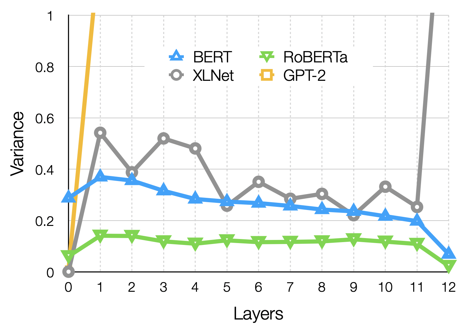
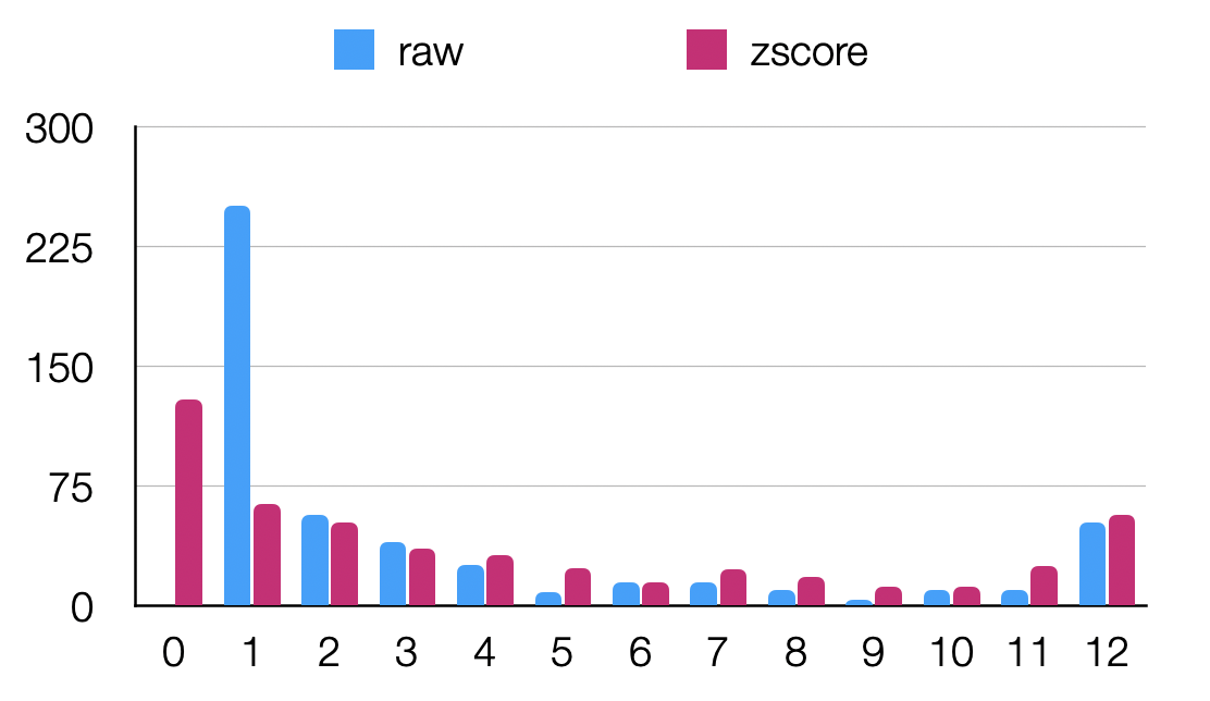
Similarly, different layers of a pre-trained model exhibit different variance patterns, particularly the first and last layers (see Figure 1222The variance of the middle layers of GPT-2 was very high. We limit the y-axis to show the pattern of variance of other models. where we plot this for several pre-trained models). When used for feature-based transfer learning, a high variance in features may result in sub-optimal and misleading results Kaufman and Rousseeuw (1990). Would normalizing the variance in contextualized embeddings be beneficial for their applications? It is important to address these questions to unwrap the full potential of contextualized embeddings when used for feature-based learning. In the context of analyzing pre-trained models, they enable a fair comparison between different layers and models.
In this paper, we make a pioneering attempt on the realm of post-processing contextual representation. To this end, we analyze the effect of four post-processing methods on contextualized embeddings. More specifically, we standardize features (individual neurons) using (i) z-score normalization (zscore), (ii) min-max normalization (minmax), and (iii) all-but-the-top (abtt) post-processing method Mu and Viswanath (2018). We also post-process word representations using unit length normalization (ulen). The first two are standard feature normalization methods shown to be an effective pre-processing step in building a successful machine learning model Jiawei Han (2011). abtt removes top principal components of contextualization representations Ethayarajh (2019) and improve isotropy of the representations. ulen has shown to be effective in improving the performance of static embedding for word similarity and analogy tasks Levy et al. (2015).
We consider contextualized embeddings of a variety of pre-trained models covering both auto-encoder and auto-regressive in design. We evaluate the effect of post-processing contextualized embeddings using various lexical-level tasks such as word similarity, word analogy, and using several sequence classification tasks from the GLUE benchmark. Our results show that:
-
•
Post-processing helps to unwrap the information present in the representations
-
•
The major improvement achieved for the last layer shows that while it is optimized for the objective function, it still possesses most of the knowledge learned in the previous layers
-
•
z-score and all-but-the-top are orthogonal and results in best performance when used in tandem for lexical tasks
-
•
z-score achieves substantial improvement on the sequence classification tasks, particularly using the representations from the middle and higher layers
We further discuss the relation between post-processing of contextualized embeddings and the research on representation analysis. In a preliminary experiment on analyzing individual neurons in pre-trained models, we show that post-processing enables a fair comparison among neurons of various layers. For example, after post-processing, we find that the last layer of BERT also has a substantial contribution towards the top neurons learning part of speech properties. Supported by our results, we recommend that normalization of a layer representation should be considered as an essential first step before using contextualized embeddings for end applications such as transfer learning and interpretation of representations.
The paper is organized as follows: Section 2 accounts for related work. Section 3 describes our approach and post-processing strategies. Section 4 presents the experimental setup. Section 5 reports our findings. We carry out the discussion supported by an application in Section 6. Section 7 concludes the paper.
2 Related Work
Static Embedding Normalization
A number of post-processing methods have been proposed to improve the performance of static embedding such as, length normalization Levy et al. (2015), centering the mean Sahlgren et al. (2016), and removing the top principal components Mu and Viswanath (2018); Arora et al. (2017). Arora et al. (2017) removed the first principal component where components are dataset specific as they compute the representations for the entire dataset. On the other hand Mu and Viswanath (2018) removed the top components by computing such representations on the entire vocabulary. They assume that higher variance components are corrupted by the information which is different than lexical semantics. Wang et al. (2019) proposed two normalization methods (i) variance normalization – normalizes the principle components of the pre-trained word vectors, (ii) dynamic embedding – learns the orthogonal latent variables from the ordered input sequence. The post-processed static representations are then evaluated on both intrinsic and extrinsic tasks, which demonstrates the effectiveness of these methods.
Contextualized Embeddings
In the context of representations of contextual pre-trained models, the effectiveness of post-processing methods have not been explored. Most of the work that uses contextualized representations use them without any pre-processing. In this work, we explore the usefulness of two commonly used post-processing methods on the embeddings extracted from pre-trained models.
Peters et al. (2018, 2019) used contextualized embeddings in feature-based setting for several sequence classification tasks. Similar to static embedding, the contextualized embeddings are used as input to an LSTM-based classifier. However, a word can have different embedding depending on the context. In addition, a plethora of work on the analysis and interpretation of deep models used feature-based approach to probe the linguistic information encoded in the representations Belinkov et al. (2017b); Conneau et al. (2018b); Liu et al. (2019a); Tenney et al. (2019b, a); Voita et al. (2019); Durrani et al. (2019); Arps et al. (2022). The most common approach uses probing classifiers Ettinger et al. (2016); Belinkov et al. (2017a); Adi et al. (2017); Conneau et al. (2018a); Hupkes et al. (2018), where a classifier is trained on a corpus of linguistic annotations using representations from the model under investigation. For example, Liu et al. (2019a) used this methodology for investigating the representations of contextual word representations on 16 linguistic tasks. Dalvi et al. (2019); Durrani et al. (2020) expanded the work on representation analysis333Please see Belinkov and Glass (2019); Sajjad et al. (2022a) for comprehensive surveys on representation analysis. to neuron-level analysis. Similar to probing classifier used in the representation analysis, they used a linear classifier with ElasticNet regularization. Recently, Sajjad et al. (2022b); Dalvi et al. (2022) introduced an unsupervised method that clusters contextualized representations of words to analyze the representations.
An orthogonal analysis comparing models and their representations relies on similarities between model representations. Bau et al. (2019) used this approach to analyze the role of individual neurons in neural machine translation. Wu et al. (2020) compared representations of several pre-trained models using various similarity methods. Another class of work on understanding the contextualized representations looked at the social bias encoded in the representations Bommasani et al. (2020).
Ethayarajh (2019) provided a different angle to the analysis of contextualized embeddings and explored the geometry of the embedding space. They showed that contextualized embeddings are anistropic and questioned the effectiveness of contextualized representations given the well known benefits of isotropic representations.
The work of Ethayarajh (2019) is in-line with ours where they studied the geometry of contextualized representations. Our work builds on top of their analysis and provides an empirical evidence supporting post-processing of embeddings. In relevance to the above mentioned studies on analyzing representation of deep models, our work has direct implications on their findings. The effect of post-processing is dependent on various factors such as, the model used for feature-based transfer learning, and the goal of the task. We suggest that post-processing particularly the z-score normalization should be considered as an essential step while designing experiments using the contextualized embeddings.
3 Approach
Consider a pre-trained model with layers .444We consider each transformer block as a layer. Let be a dataset composed of words of interest, . Our model encodes input tokens depending on their context. We first normalize each contextualized embedding using various post-processing methods. For each word , we then form a single representation, similar to a static embedding, for every layer in . We evaluate the word representation on lexical-level tasks and sequence classification tasks. In the latter, we train a BiLSTM classifier pre-initialized with our processed embedding.
3.1 Word Representations
Let be a sentence containing the word . Let represents the contextual embedding from layer of model for the word , with the given context , specifically,
| (1) |
where is a shorthand for the contextual embeddings for all tokens in , from which we pick only one that is relevant to the word of interest , and further index into a specific layer . is the number of features (i.e., size of the hidden dimension in a layer), which is per layer in the models analyzed in this paper.
In order to form a single representation for each word,555We form a single representation to limit the number of tokens. In Section 6, we use contextualized embedding of a word in the application. Our results show that our findings generalize to both static and contextualized embeddings. we first extract contextual embeddings for each word in at least contexts. These contexts are derived from a large corpus of sentences,666We used Wikipedia dump collected on 3rd February 2020. and are randomly chosen from all sentences containing the word . We also employ an upper limit for the maximum number of contexts used for any word, to avoid the dominance of frequent words such as closed class words. In our analysis, is set to and is set to . Thus, each word in our dataset will then have between and contextual embeddings extracted from the model . We then aggregate these contextual embeddings by mean pooling each dimension:
| (2) |
where is the number of contexts (sentences) the word was present in.
3.2 Post-processing Methods
We perform four kinds of post-processing on the representations before aggregating them into . They are; (i) z-score normalization, (ii) min-max normalization, (iii) unit length, and (iv) all-but-the-top normalization. The former two are common feature normalization methods used in machine learning.777https://en.wikipedia.org/wiki/Feature_scaling The latter two have shown to be effective in post-processing static embedding. All of these post-processing methods except unit length are applied at the feature-level which is a neuron (single dimension) in our case. The unit length is applied for each word representation.
Let represents the set of all word occurrence embeddings ’s for all words in the dataset .
z-score Normalization (zscore)
Centering and scaling input vectors to have zero-mean and unit-variance is a common pre-processing practice in many machine learning pipelines. Concretely, each feature’s (in our case 1 of 768 dimensions from each layer’s representation) mean and variance is computed across all words in our dataset , followed by subtraction of the mean and division of the standard deviation for each of the feature’s value for each embedding .
| (3) |
where is the post-processed representation of word in context from layer .
Min-max Normalization (minmax)
The min-max normalization rescales each feature range between 0 and 1. Given values of a feature, minmax is calculated as follows:
| (4) |
where and represent the minimum and maximum values of feature .
Unit Length (ulen)
The normalization of word vectors to unit length is shown to be effective for static embedding Levy et al. (2015). Here, we evaluate its efficacy for contextualized embeddings. Different from other post-processing methods mentioned in this work where we normalize each feature, ulen is applied at each word vector i.e., a set of features that represent a vector. We normalize vectors using norm.
All-but-the-top (abtt)
Mu and Viswanath (2018) showed that all word representations share a large common vector and similar dominating directions which influence them. Eliminating such directions yields isotropic word representations with better self-normalization properties.
We hypothesize that contextualized embeddings belonging to different layers might be influenced by various design factors e.g., initial layers of BERT may have a strong influence of position embedding, Kovaleva et al. (2019) showed that the last layer of BERT is optimized for the objective function. These factors if dominating the contextual representations may result in sub-optimal performance. We apply abtt to eliminate such kind of dominating directions.
4 Training and Evaluation Setup
Data
We used the Wikipedia dump of 124 million sentences collected on 3rd February 2020. We tokenized the text using the Moses tokenizer Koehn et al. (2007). Given a pretrained model, we extracted the contextualized embedding of words from the Wikipedia corpus and generated a single word representation as described in Section 3.1.
Contextualized models
Lexical-level tasks
We used seven word similarity datasets: WordSim353 split into similarity and relatedness Zesch et al. (2008); Agirre et al. (2009), MEN Bruni et al. (2012), Mechanical Turk Radinsky et al. (2011), Rare Words Luong et al. (2013), SimLex-999 Hill et al. (2015) and RG65 Rubenstein and Goodenough (1965). The datasets contain a word pair with their human annotated similarity scores. The quality of a word embedding is calculated based on the cosine similarity score between a given pair of words, in comparison with their human-provided scores.
Moreover, we used three analogy datasets: MSR Mikolov et al. (2013b), Google Mikolov et al. (2013a) and SemEval2012-2 Jurgens et al. (2012). The analogy tasks involve predicting a word given an analogy relationship like “a is to b” as “c is to d” where d is the word to predict. For more details on each task, we refer the reader to Levy et al. (2015). We used the word embedding benchmark toolkit888https://github.com/kudkudak/word-embeddings-benchmarks to evaluate word representations on the word analogy and word similarity tasks.
Sequence classification tasks
We evaluated using six General Language Understanding Evaluation (GLUE) tasks (Wang et al., 2018):999See Appendix for data statistics and download link. SST-2 for sentiment analysis with the Stanford sentiment treebank Socher et al. (2013), MNLI for natural language inference Williams et al. (2018), QNLI for Question NLI Rajpurkar et al. (2016), RTE for recognizing textual entailment Bentivogli et al. (2009), MRPC for Microsoft Research paraphrase corpus Dolan and Brockett (2005), and STS-B for the semantic textual similarity benchmark Cer et al. (2017). We compute statistical significance in performance differences using McNemar test.
We trained a BiLSTM model using Jiant Phang et al. (2020), with the following parameters settings: vocabulary size 30k, sequence length 150 words, batch size 32, dropout 0.2, hidden layer size 1024, number of layers 2, AMSGRAD, learning rate decay 0.99, minimum learning rate 1e-06. The embedding layer is of size 768 for all experiments.

5 Analysis and Findings
We experiment with four post-processing methods as mentioned in Section 3.2. We analyze the effect of each post-processing using lexical and sequence classification tasks. Due to limited space, we present the average results of three models only. The task-wise results of all models including GPT2 are provided in Appendix D and C. We did not observe any difference in task-specific trends compared to the average trend present in the paper.
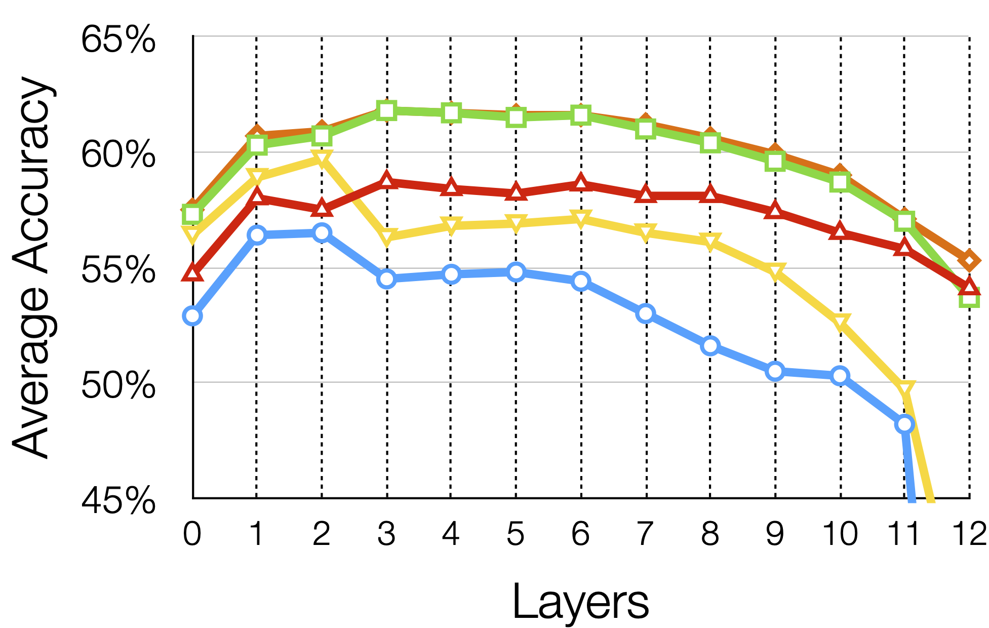
5.1 Lexical-level Tasks
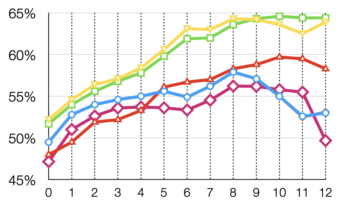
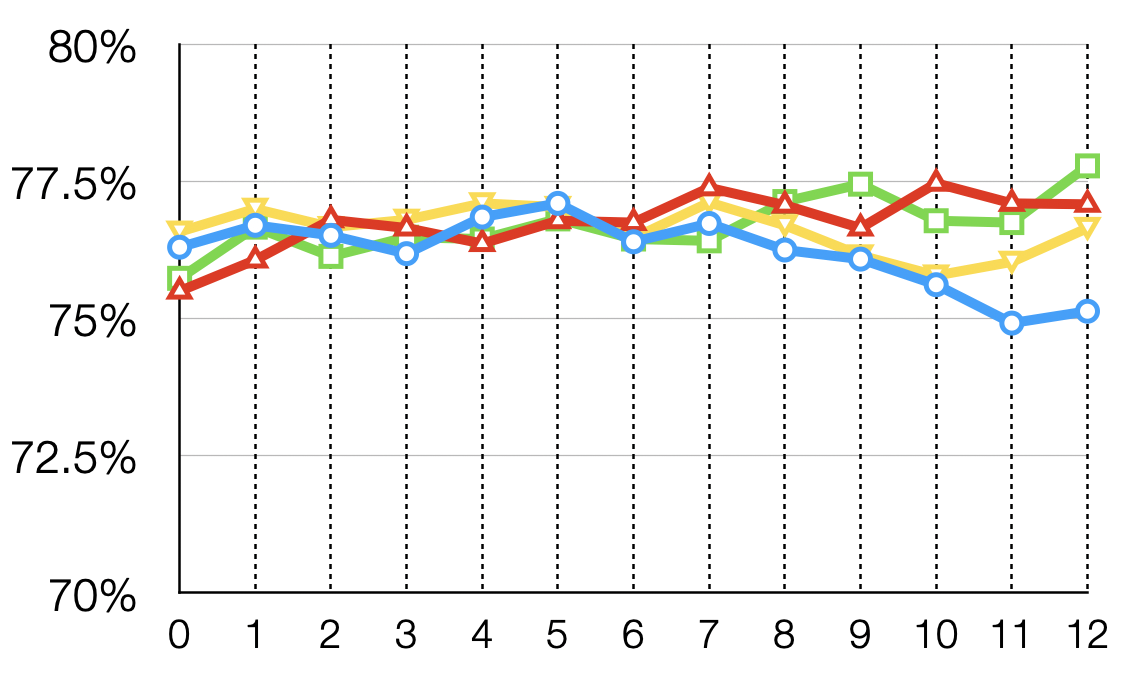
Figure 2 presents the average layer-wise results using the lexical tasks. raw represents the embedding before applying any post-processing.
Post-processing is generally helpful. Comparing raw (blue line) with the rest, other than a few exceptions, layers of all models benefited from the post-processing steps. Surprisingly, ulen did not result in any change in the performance compared to raw.101010The results of ulen and raw were identical up to two decimal points. The line of ulen is not visible because it is hidden behind raw in the figure. minmax resulted in poor performance than raw. The two promising post-processing methods are zscore and abtt. In the following, we mainly discuss the results of zscore and abtt.
Higher layers achieve major improvements in performance. The general performance trend from lower layers to higher layers suggest that it is essential to post-process the representations of higher layers in order to unwrap the information present in those layers for the lexical tasks. In other words, the higher layer representations though optimized for the objective function still possess similar or better lexical-level information compared to the lower layers.
Comparing post-processing combinations. With the exception of the lower layers of BERT and the last two layers of RoBERTa, zscore (red line) achieved competitive or better performance than using the raw (blue line) representations. Comparing the variance of each layer (Figure 1), zscore is very effective for high variance layers such as the last layer of XLNet and most of the layers of GPT2 (see Appendix B). While RoBERTa has the most smooth variance curve, zscore is still quite effective in improving the performance from layer 1 to 10. The sudden drop in the performance of the last two layers is surprising. The reason could be an extremely low variance of these layers as can be seen in Figure 1 and applying zscore alone amplifies the amount of noise.
abtt outperformed or is competitive to the best performing individual post-processing methods (yellow line in Figure 2). The consistent improvement across all models for the lower layers reflects that the lower layer representations consist of top principle components that negatively influence the representations in the context of lexical tasks. For example, the representations from the lower layers of BERT might have a strong influence of position embeddings which may be harmful for word similarity and analogy tasks. On the top two layers, abtt does not seem to be very effective on RoBERTa and XLNet suggesting fewer dominating principle components in the higher layers.
Since zscore and abtt targets different properties in the representation, we apply them in succession. Using both methods in any order resulted in better representation quality especially for the higher layers (see green line abtt+zscore that outperformed or has competitive performance to the best result on all layers). These results show the potential of combining various post-processing methods, like abtt+zscore, in achieving better performance on the lexical tasks.
Comparing models. While post-processing methods benefited all models, XLNet showed the most increase in the performance with lower-middle layers (3,4) and higher layers outperforming all layers across all models. BERT also showed similar gains with more consistent trend i.e. an increase in performance with every higher layer. We did observe gains for RoBERTa. However, they are less substantial compared to BERT and the results on last layer dropped compared to other layers.

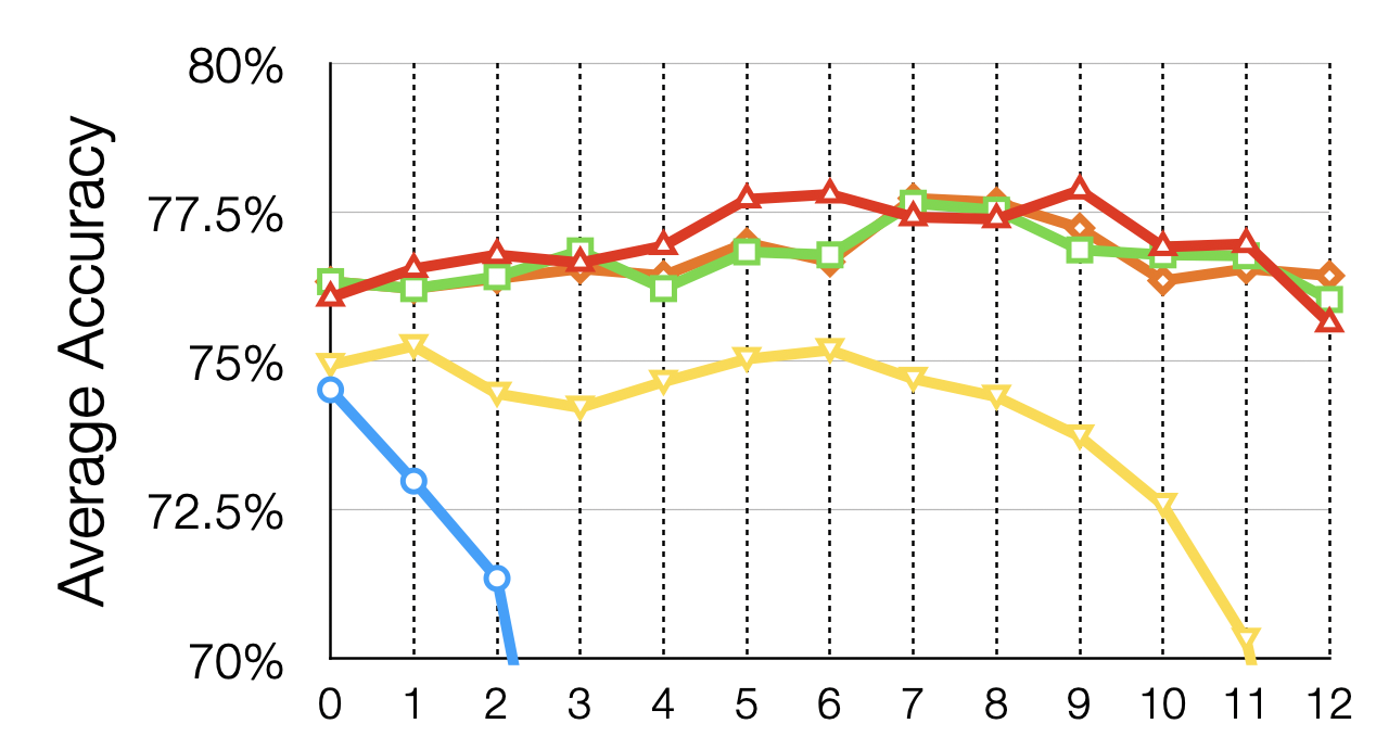
5.2 Sequence classification Tasks
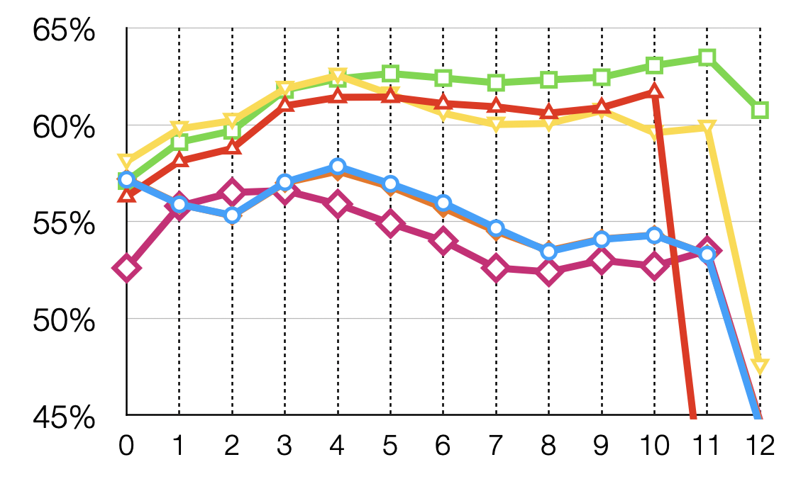
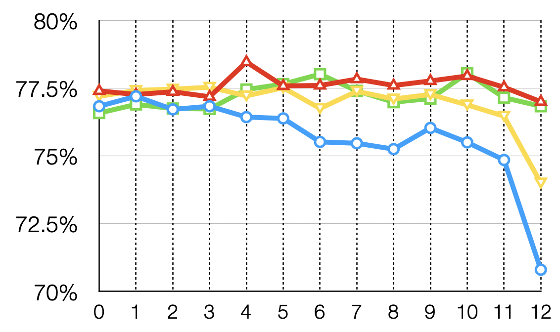
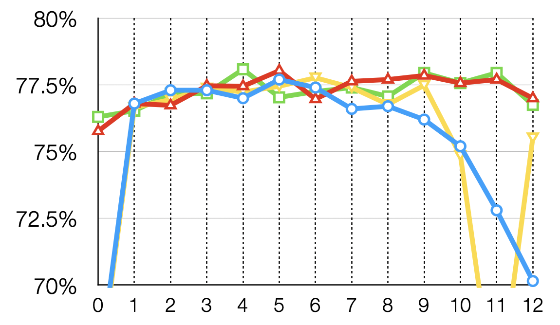
Figure 3 presents the average layer-wise results using six GLUE tasks.111111We observed similar trends for GPT2 (see Appendix B). The performance improvements when post-processing the higher layers are found to be statistically significant at p=0.05. Additionally, the embedding layer of XLNet and middle to higher layers of RoBERTa achieved statistically significant improvements. Due to the poor performance of ulen and minmax, we did not report and discuss their results.
Post-processing is generally helpful. Similar to the performance on the lexical tasks, we observed that zscore and abtt post-processing methods resulted in competitive or better performance than raw. Particularly, zscore substantially improved the performance of the middle and higher layers (see red line and blue line representing zscore and raw respectively). abtt has comparable or better results than raw, although it never outperformed zscore. An interesting observation is the embedding layer where abtt resulted in similar performance to raw across all models. The embedding layer may encode information related to word identity and position, as in the case of BERT and RoBERTa which is neither useful nor harmful for the downstream tasks. abtt removed these high principle components while maintaining the performance of the embedding layer. Combining both post-processings did not result in any consistent benefit over using zscore alone.
All layers possess information about the tasks. In contrast to the common notion Kovaleva et al. (2019) that the last layer is optimized for the objective function, and hence it is sub-optimal to use for down-stream tasks, we found that after zscore, the results of the last layers substantially improved, showing competitive results to the best performing layer for each model.
Task-wise performance Overall, majority of the tasks showed significant improvement with the post-processing of higher-layers. Additionally the embedding layer of XLNet benefited substantially with zscore. For example, the QNLI performance improved from 69.6 to 80.7 for the embedding layer, and 66.6 to 82.2 for the last layer. The only exception is the SST task that showed minimum benefit of the post-processing methods across all models. The performance differences between raw and post-processing methods are within 1% range, and are found to be insignificant.
6 Application and Discussion
The effectiveness of the post-processing of representations, particularly zscore, raises several interesting points in relation to the studies that use contextualized representations like feature-based transfer learning Dalvi et al. (2020) and analysis/interpretation of deep models. For example, the work on probing layer representations typically builds a linear classifier and uses the classifier’s performance as a proxy to judge how much linguistic information is learned in the representation. Our results show that even when using a strong classification model based on BiLSTM, it is essential to normalize the representations before training. A linear classifier is likely to be more vulnerable to the variance in the features and may not capture the true potential present in the representation. Similarly, feature-based transfer learning is directly affected by this post-processing and is likely to improve performance as shown by our sequence classification results.
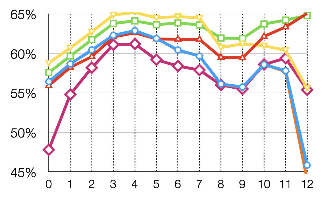
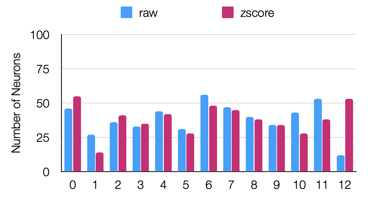
In order to probe whether the post-processing of representations would impact representation analysis, we conducted a preliminary experiment on analyzing individual neurons in pre-trained models. Durrani et al. (2020) used the Linguistic Correlation Analysis (LCA) method to identify a set of neurons with respect to a linguistic property. The method trains a linear classifier on the linguistic property of interest while using neurons of the pre-trained model as features (12 layers x 768 dimensions = 9984 features). The output of the method results in a list of salient neurons with respect to the property in hand. We consider part-of-speech tagging (POS) as our linguistic property of interest and reproduce their results using the raw and the zscore post-processed contextualized embeddings of BERT and XLNet. Since LCA considers contextualized embeddings, we did not aggregate the contextualized embeddings of a word into a single word embedding as describe in Section 3.1. Thus, we use the contextualized embedding extracted from pre-trained models directly in the training of the linear classifier.
Figure 4 presents the layer-wise distribution of salient neurons identified by the algorithm using raw and zscore contextualized embeddings. On BERT, the most surprising result is the contribution of last layer which was minimum in the case of raw but after zscore, it is among the top contributing layers from which the most salient POS neurons are selected. The results of XLNet are also interesting. The contribution of embedding layer’s neuron (0 index on x-axis) is zero in the case of raw contextualized embeddings while the first layer dominates the distribution. The zscore contextualized embedding picked the most number of salient neurons from the embedding layer and selected relatively less neurons from the first layer. This result shows that any analysis obtained by applying external probes on the features generated from pre-trained models needs to consider the effect of normalization into account as it provides an alternative view. In the future, we plan to extend this investigation further by analyzing the effect of post-processing on various other similarity and interpretation analysis works.
While the benefits of post-processing is evident in our experiments, the choice of when to use post-processing is application dependent. In analyzing representations of a network using a classification model, it is recommended to have standardized features to learn the best model. The choice of learned model architecture also plays a role here. The methods invariant to affine transformations would be least effected by the variability of features Kaufman and Rousseeuw (1990). For other applications e.g., identifying the importance of a neuron in a pre-trained model, the variance in the values of a neuron can be a signal of its importance and post-processing like zscore would result in the loss of such information.
7 Conclusion
We analyzed the effect of four post-processing methods on the contextualized representations using both the lexical and sequence classification tasks. We showed that for lexical tasks, post-processing methods zscore and abtt are essential to achieve better performance. On the sequence classification tasks, zscore alone outperformed all post-processing methods and raw. The most astonishing results are the large improvements in the performance of the last layers which reflect that they also possess equal amount of information about the lexical and classification tasks but the information is not readily available when used in feature-based transfer learning.
Our work opens several interesting frontiers with respect to the work that uses contextualized representations. In a preliminary experiment on representation analysis, we showed that post-processing the representations resulted in different findings. We suggested zscore as an essential step to consider when using contextualized embeddings for the feature-based transfer learning.
Ethics and Broader Impact
We used publicly available datasets, following their terms in the licenses. This includes seven datasets for similarity tasks, three datasets for analogy tasks, and six GLUE datasets. We do not see any harm or ethical issues resulting from our study and findings. Our study benefits the feature-based transfer learning at large and has direct implications towards the work on interpreting and analyzing deep models.
References
- Adi et al. (2017) Yossi Adi, Einat Kermany, Yonatan Belinkov, Ofer Lavi, and Yoav Goldberg. 2017. Fine-grained analysis of sentence embeddings using auxiliary prediction tasks. In Proceedings of the Internaltional Confernece for Learning Representations (ICLR).
- Agirre et al. (2009) Eneko Agirre, Enrique Alfonseca, Keith Hall, Jana Kravalova, Marius Paşca, and Aitor Soroa. 2009. A study on similarity and relatedness using distributional and WordNet-based approaches. In Proceedings of Human Language Technologies: The 2009 Annual Conference of the North American Chapter of the Association for Computational Linguistics, pages 19–27, Boulder, Colorado. Association for Computational Linguistics.
- Arora et al. (2017) Sanjeev Arora, Yingyu Liang, and Tengyu Ma. 2017. A simple but tough-to-beat baseline for sentence embeddings. In Proceedings of the International Conference on Learning Representations.
- Arps et al. (2022) David Arps, Younes Samih, Laura Kallmeyer, and Hassan Sajjad. 2022. Probing for constituency structure in neural language models.
- Bau et al. (2019) D. Anthony Bau, Yonatan Belinkov, Hassan Sajjad, Nadir Durrani, Fahim Dalvi, and James Glass. 2019. Identifying and controlling important neurons in neural machine translation. In International Conference on Learning Representations (ICLR).
- Belinkov et al. (2017a) Yonatan Belinkov, Nadir Durrani, Fahim Dalvi, Hassan Sajjad, and James Glass. 2017a. What do Neural Machine Translation Models Learn about Morphology? In Proceedings of the 55th Annual Meeting of the Association for Computational Linguistics (ACL), Vancouver. Association for Computational Linguistics.
- Belinkov et al. (2020) Yonatan Belinkov, Nadir Durrani, Fahim Dalvi, Hassan Sajjad, and James Glass. 2020. On the linguistic representational power of neural machine translation models. Computational Linguistics, 46(1):1–52.
- Belinkov and Glass (2019) Yonatan Belinkov and James Glass. 2019. Analysis methods in neural language processing: A survey. Transactions of the Association for Computational Linguistics, 7:49–72.
- Belinkov et al. (2017b) Yonatan Belinkov, Lluís Màrquez, Hassan Sajjad, Nadir Durrani, Fahim Dalvi, and James Glass. 2017b. Evaluating layers of representation in neural machine translation on part-of-speech and semantic tagging tasks. In Proceedings of the Eighth International Joint Conference on Natural Language Processing (Volume 1: Long Papers), pages 1–10, Taipei, Taiwan. Asian Federation of Natural Language Processing.
- Bentivogli et al. (2009) Luisa Bentivogli, Ido Dagan, Hoa Trang Dang, Danilo Giampiccolo, and Bernardo Magnini. 2009. The fifth pascal recognizing textual entailment challenge. In In Proc Text Analysis Conference (TAC’09.
- Bommasani et al. (2020) Rishi Bommasani, Kelly Davis, and Claire Cardie. 2020. Interpreting Pretrained Contextualized Representations via Reductions to Static Embeddings. In Proceedings of the 58th Annual Meeting of the Association for Computational Linguistics, pages 4758–4781, Online. Association for Computational Linguistics.
- Bruni et al. (2012) Elia Bruni, Gemma Boleda, Marco Baroni, and Nam-Khanh Tran. 2012. Distributional semantics in technicolor. In Proceedings of the 50th Annual Meeting of the Association for Computational Linguistics (Volume 1: Long Papers), pages 136–145, Jeju Island, Korea. Association for Computational Linguistics.
- Cer et al. (2017) Daniel Cer, Mona Diab, Eneko Agirre, Iñigo Lopez-Gazpio, and Lucia Specia. 2017. SemEval-2017 task 1: Semantic textual similarity multilingual and crosslingual focused evaluation. In Proceedings of the 11th International Workshop on Semantic Evaluation (SemEval-2017), pages 1–14, Vancouver, Canada. Association for Computational Linguistics.
- Conneau et al. (2018a) Alexis Conneau, German Kruszewski, Guillaume Lample, Loïc Barrault, and Marco Baroni. 2018a. What you can cram into a single $&!#* vector: Probing sentence embeddings for linguistic properties. In Proceedings of the 56th Annual Meeting of the Association for Computational Linguistics (Volume 1: Long Papers), pages 2126–2136, Melbourne, Australia. Association for Computational Linguistics.
- Conneau et al. (2018b) Alexis Conneau, German Kruszewski, Guillaume Lample, Loïc Barrault, and Marco Baroni. 2018b. What you can cram into a single vector: Probing sentence embeddings for linguistic properties. In Proceedings of the 56th Annual Meeting of the Association for Computational Linguistics (ACL).
- Dalvi et al. (2019) Fahim Dalvi, Nadir Durrani, Hassan Sajjad, Yonatan Belinkov, D. Anthony Bau, and James Glass. 2019. What is one grain of sand in the desert? analyzing individual neurons in deep nlp models. In Proceedings of the Thirty-Third AAAI Conference on Artificial Intelligence (AAAI, Oral presentation).
- Dalvi et al. (2017) Fahim Dalvi, Nadir Durrani, Hassan Sajjad, Yonatan Belinkov, and Stephan Vogel. 2017. Understanding and improving morphological learning in the neural machine translation decoder. In Proceedings of the Eighth International Joint Conference on Natural Language Processing (Volume 1: Long Papers), pages 142–151, Taipei, Taiwan. Asian Federation of Natural Language Processing.
- Dalvi et al. (2022) Fahim Dalvi, Abdul Rafae Khan, Firoj Alam, Nadir Durrani, Jia Xu, and Hassan Sajjad. 2022. Discovering latent concepts learned in BERT. In International Conference on Learning Representations.
- Dalvi et al. (2020) Fahim Dalvi, Hassan Sajjad, Nadir Durrani, and Yonatan Belinkov. 2020. Analyzing redundancy in pretrained transformer models. In Proceedings of the 2020 Conference on Empirical Methods in Natural Language Processing (EMNLP), pages 4908–4926, Online. Association for Computational Linguistics.
- Devlin et al. (2019) Jacob Devlin, Ming-Wei Chang, Kenton Lee, and Kristina Toutanova. 2019. BERT: pre-training of deep bidirectional transformers for language understanding. In Proceedings of the 2019 Conference of the North American Chapter of the Association for Computational Linguistics: Human Language Technologies, NAACL-HLT 2019, Minneapolis, MN, USA, June 2-7, 2019, Volume 1 (Long and Short Papers), pages 4171–4186. Association for Computational Linguistics.
- Dolan and Brockett (2005) William B. Dolan and Chris Brockett. 2005. Automatically constructing a corpus of sentential paraphrases. In Proceedings of the Third International Workshop on Paraphrasing (IWP2005).
- Durrani et al. (2019) Nadir Durrani, Fahim Dalvi, Hassan Sajjad, Yonatan Belinkov, and Preslav Nakov. 2019. One size does not fit all: Comparing NMT representations of different granularities. In Proceedings of the 2019 Conference of the North American Chapter of the Association for Computational Linguistics: Human Language Technologies, Volume 1 (Long and Short Papers), pages 1504–1516, Minneapolis, Minnesota. Association for Computational Linguistics.
- Durrani et al. (2020) Nadir Durrani, Hassan Sajjad, Fahim Dalvi, and Yonatan Belinkov. 2020. Analyzing individual neurons in pretrained language models. In Proceedings of the 2020 Conference on Empirical Methods in Natural Language Processing (EMNLP-2020), Online. Association for Computational Linguistics.
- Ethayarajh (2019) Kawin Ethayarajh. 2019. How contextual are contextualized word representations? comparing the geometry of BERT, ELMo, and GPT-2 embeddings. In Proceedings of the 2019 Conference on Empirical Methods in Natural Language Processing and the 9th International Joint Conference on Natural Language Processing (EMNLP-IJCNLP), pages 55–65, Hong Kong, China. Association for Computational Linguistics.
- Ettinger et al. (2016) Allyson Ettinger, Ahmed Elgohary, and Philip Resnik. 2016. Probing for semantic evidence of composition by means of simple classification tasks. In Proceedings of the 1st Workshop on Evaluating Vector-Space Representations for NLP, pages 134–139, Berlin, Germany. Association for Computational Linguistics.
- Hill et al. (2015) Felix Hill, Roi Reichart, and Anna Korhonen. 2015. SimLex-999: Evaluating semantic models with (genuine) similarity estimation. Computational Linguistics, 41(4):665–695.
- Hupkes et al. (2018) Dieuwke Hupkes, Sara Veldhoen, and Willem Zuidema. 2018. Visualisation and ‘diagnostic classifiers’ reveal how recurrent and recursive neural networks process hierarchical structure. Journal of Artificial Intelligence Research, 61:907–926.
- Jiawei Han (2011) Micheline Kamber Jiawei Han, Jian Pei. 2011. Data Mining: Concepts and Techniques. Elsevier Science Ltd.
- Jurgens et al. (2012) David A. Jurgens, Peter D. Turney, Saif M. Mohammad, and Keith J. Holyoak. 2012. Semeval-2012 task 2: Measuring degrees of relational similarity. In Proceedings of the First Joint Conference on Lexical and Computational Semantics - Volume 1: Proceedings of the Main Conference and the Shared Task, and Volume 2: Proceedings of the Sixth International Workshop on Semantic Evaluation, SemEval ’12, page 356–364, USA. Association for Computational Linguistics.
- Kaufman and Rousseeuw (1990) Leonard Kaufman and Peter J. Rousseeuw. 1990. Finding Groups in Data: An Introduction to Cluster Analysis. John Wiley.
- Koehn et al. (2007) Philipp Koehn, Hieu Hoang, Alexandra Birch, Chris Callison-Burch, Marcello Federico, Nicola Bertoldi, Brooke Cowan, Wade Shen, Christine Moran, Richard Zens, et al. 2007. Moses: Open source toolkit for statistical machine translation. In Proceedings of the 45th annual meeting of the ACL on interactive poster and demonstration sessions, pages 177–180. Association for Computational Linguistics.
- Kovaleva et al. (2019) Olga Kovaleva, Alexey Romanov, Anna Rogers, and Anna Rumshisky. 2019. Revealing the dark secrets of BERT. In Proceedings of the 2019 Conference on Empirical Methods in Natural Language Processing and the 9th International Joint Conference on Natural Language Processing (EMNLP-IJCNLP), pages 4365–4374, Hong Kong, China. Association for Computational Linguistics.
- Levy et al. (2015) Omer Levy, Yoav Goldberg, and Ido Dagan. 2015. Improving distributional similarity with lessons learned from word embeddings. Transactions of the Association for Computational Linguistics, 3:211–225.
- Liu et al. (2019a) Nelson F. Liu, Matt Gardner, Yonatan Belinkov, Matthew E. Peters, and Noah A. Smith. 2019a. Linguistic knowledge and transferability of contextual representations. In Proceedings of the 2019 Conference of the North American Chapter of the Association for Computational Linguistics: Human Language Technologies, Volume 1 (Long and Short Papers), pages 1073–1094, Minneapolis, Minnesota. Association for Computational Linguistics.
- Liu et al. (2019b) Yinhan Liu, Myle Ott, Naman Goyal, Jingfei Du, Mandar Joshi, Danqi Chen, Omer Levy, Mike Lewis, Luke Zettlemoyer, and Veselin Stoyanov. 2019b. RoBERTa: A robustly optimized BERT pretraining approach. CoRR, abs/1907.11692.
- Luong et al. (2013) Thang Luong, Richard Socher, and Christopher Manning. 2013. Better word representations with recursive neural networks for morphology. In Proceedings of the Seventeenth Conference on Computational Natural Language Learning, pages 104–113, Sofia, Bulgaria. Association for Computational Linguistics.
- Mikolov et al. (2013a) Tomas Mikolov, Kai Chen, Greg S. Corrado, and Jeffrey Dean. 2013a. Efficient estimation of word representations in vector space.
- Mikolov et al. (2013b) Tomas Mikolov, Scott Wen-tau Yih, and Geoffrey Zweig. 2013b. Linguistic regularities in continuous space word representations. In Proceedings of the 2013 Conference of the North American Chapter of the Association for Computational Linguistics: Human Language Technologies (NAACL-HLT-2013). Association for Computational Linguistics.
- Mu and Viswanath (2018) Jiaqi Mu and Pramod Viswanath. 2018. All-but-the-top: Simple and effective postprocessing for word representations. In International Conference on Learning Representations.
- Peters et al. (2018) Matthew Peters, Mark Neumann, Mohit Iyyer, Matt Gardner, Christopher Clark, Kenton Lee, and Luke Zettlemoyer. 2018. Deep contextualized word representations. In Proceedings of the 2018 Conference of the North American Chapter of the Association for Computational Linguistics: Human Language Technologies, Volume 1 (Long Papers), pages 2227–2237, New Orleans, Louisiana. Association for Computational Linguistics.
- Peters et al. (2019) Matthew E. Peters, Sebastian Ruder, and Noah A. Smith. 2019. To tune or not to tune? adapting pretrained representations to diverse tasks. In Proceedings of the 4th Workshop on Representation Learning for NLP (RepL4NLP-2019), pages 7–14, Florence, Italy. Association for Computational Linguistics.
- Phang et al. (2020) Jason Phang, Phil Yeres, Jesse Swanson, Haokun Liu, Ian F. Tenney, Phu Mon Htut, Clara Vania, Alex Wang, and Samuel R. Bowman. 2020. jiant 2.0: A software toolkit for research on general-purpose text understanding models. http://jiant.info/.
- Radford et al. (2018) Alec Radford, Karthik Narasimhan, Tim Salimans, and Ilya Sutskever. 2018. Improving language understanding by generative pre-training.
- Radford et al. (2019) Alec Radford, Jeffrey Wu, Rewon Child, David Luan, Dario Amodei, and Ilya Sutskever. 2019. Language models are unsupervised multitask learners. OpenAI blog, 1(8):9.
- Radinsky et al. (2011) Kira Radinsky, Eugene Agichtein, Evgeniy Gabrilovich, and Shaul Markovitch. 2011. A word at a time: Computing word relatedness using temporal semantic analysis. In Proceedings of the 20th International Conference on World Wide Web, WWW ’11, page 337–346, New York, NY, USA. Association for Computing Machinery.
- Rajpurkar et al. (2016) Pranav Rajpurkar, Jian Zhang, Konstantin Lopyrev, and Percy Liang. 2016. SQuAD: 100,000+ questions for machine comprehension of text. In Proceedings of the 2016 Conference on Empirical Methods in Natural Language Processing, pages 2383–2392, Austin, Texas. Association for Computational Linguistics.
- Rubenstein and Goodenough (1965) Herbert Rubenstein and John B. Goodenough. 1965. Contextual correlates of synonymy. Commun. ACM, 8(10):627–633.
- Sahlgren et al. (2016) Magnus Sahlgren, Amaru Cuba Gyllensten, Fredrik Espinoza, Ola Hamfors, Jussi Karlgren, Fredrik Olsson, Per Persson, Akshay Viswanathan, and Anders Holst. 2016. The gavagai living lexicon. In Proceedings of the Tenth International Conference on Language Resources and Evaluation (LREC’16), pages 344–350, Portorož, Slovenia. European Language Resources Association (ELRA).
- Sajjad et al. (2022a) Hassan Sajjad, Nadir Durrani, and Fahim Dalvi. 2022a. Neuron-level Interpretation of Deep NLP Models: A Survey. Transactions of the Association for Computational Linguistics.
- Sajjad et al. (2022b) Hassan Sajjad, Nadir Durrani, Fahim Dalvi, Firoj Alam, Abdul Rafae Khan, and Jia Xu. 2022b. Analyzing encoded concepts in transformer language models. In Proceedings of the 2022 Conference of the North American Chapter of the Association for Computational Linguistics, NAACL ’22, Seattle, Washington, USA. Association for Computational Linguistics.
- Socher et al. (2013) Richard Socher, Alex Perelygin, Jean Wu, Jason Chuang, Christopher D. Manning, Andrew Ng, and Christopher Potts. 2013. Recursive deep models for semantic compositionality over a sentiment treebank. In Proceedings of the 2013 Conference on Empirical Methods in Natural Language Processing, pages 1631–1642, Seattle, Washington, USA. Association for Computational Linguistics.
- Tenney et al. (2019a) Ian Tenney, Dipanjan Das, and Ellie Pavlick. 2019a. BERT rediscovers the classical NLP pipeline. In Proceedings of the 57th Annual Meeting of the Association for Computational Linguistics, pages 4593–4601, Florence, Italy. Association for Computational Linguistics.
- Tenney et al. (2019b) Ian Tenney, Patrick Xia, Berlin Chen, Alex Wang, Adam Poliak, R Thomas McCoy, Najoung Kim, Benjamin Van Durme, Samuel R. Bowman, Dipanjan Das, and Ellie Pavlick. 2019b. What do you learn from context? probing for sentence structure in contextualized word representations.
- Voita et al. (2019) Elena Voita, David Talbot, Fedor Moiseev, Rico Sennrich, and Ivan Titov. 2019. Analyzing multi-head self-attention: Specialized heads do the heavy lifting, the rest can be pruned. In Proceedings of the 57th Annual Meeting of the Association for Computational Linguistics, pages 5797–5808, Florence, Italy. Association for Computational Linguistics.
- Wang et al. (2018) Alex Wang, Amanpreet Singh, Julian Michael, Felix Hill, Omer Levy, and Samuel Bowman. 2018. GLUE: A multi-task benchmark and analysis platform for natural language understanding. In Proceedings of the 2018 EMNLP Workshop BlackboxNLP: Analyzing and Interpreting Neural Networks for NLP, pages 353–355, Brussels, Belgium. Association for Computational Linguistics.
- Wang et al. (2019) B. Wang, F. Chen, A. Wang, and C. . J. Kuo. 2019. Post-processing of word representations via variance normalization and dynamic embedding. In 2019 IEEE International Conference on Multimedia and Expo (ICME), pages 718–723.
- Williams et al. (2018) Adina Williams, Nikita Nangia, and Samuel Bowman. 2018. A broad-coverage challenge corpus for sentence understanding through inference. In Proceedings of the 2018 Conference of the North American Chapter of the Association for Computational Linguistics: Human Language Technologies, Volume 1 (Long Papers), pages 1112–1122, New Orleans, Louisiana. Association for Computational Linguistics.
- Wilson and Schakel (2015) Benjamin J. Wilson and Adriaan M. J. Schakel. 2015. Controlled experiments for word embeddings. CoRR, abs/1510.02675.
- Wu et al. (2020) John Wu, Yonatan Belinkov, Hassan Sajjad, Nadir Durrani, Fahim Dalvi, and James Glass. 2020. Similarity Analysis of Contextual Word Representation Models. In Proceedings of the 58th Annual Meeting of the Association for Computational Linguistics (ACL), Seattle. Association for Computational Linguistics.
- Yang et al. (2019) Zhilin Yang, Zihang Dai, Yiming Yang, Jaime Carbonell, Russ R Salakhutdinov, and Quoc V Le. 2019. Xlnet: Generalized autoregressive pretraining for language understanding. In Advances in neural information processing systems, pages 5753–5763.
- Zesch et al. (2008) Torsten Zesch, Christof Müller, and Iryna Gurevych. 2008. Using wiktionary for computing semantic relatedness. In Proceedings of the 23rd National Conference on Artificial Intelligence - Volume 2, AAAI’08, page 861–866. AAAI Press.
Appendix
Appendix A Data Statistics
In table 1, we present statistics of the different datasets that we used for the experiments.
| Task | Train | Dev | Task | Train | Dev |
|---|---|---|---|---|---|
| SST-2 | 67,349 | 872 | QQP | 363,846 | 40,430 |
| MRPC | 3,668 | 408 | RTE | 2,490 | 277 |
| MNLI | 392,702 | 9,815 | STS-B | 5,749 | 1,500 |
| QNLI | 104,743 | 5,463 |
Appendix B GPT-2 Average Results on GLUE
In Figure 5(a) and 5(b), we report the average results for different GLUE and lexical tasks across different L/Ns, respectively.
Appendix C Sequence Classification Results
In the following tables, we provide results obtained from raw embedding, z-socre normalization and all-but-the-top, for BERT: 2, 3, 4; XLNet: 5, 6, 7; RoBERTa: 9, 10 and GPT2: 11, 12, 13.
| L/N | QNLI | MNLI | MRPC | SST | STS | RTE | RTE |
|---|---|---|---|---|---|---|---|
| 0 | 0.82 | 0.724 | 0.775 | 0.88 | 0.801 | 0.578 | 0.578 |
| 1 | 0.815 | 0.724 | 0.797 | 0.885 | 0.8 | 0.581 | 0.581 |
| 2 | 0.816 | 0.712 | 0.784 | 0.89 | 0.808 | 0.581 | 0.581 |
| 3 | 0.805 | 0.716 | 0.779 | 0.894 | 0.807 | 0.57 | 0.57 |
| 4 | 0.818 | 0.734 | 0.775 | 0.89 | 0.806 | 0.588 | 0.588 |
| 5 | 0.824 | 0.74 | 0.779 | 0.901 | 0.804 | 0.578 | 0.578 |
| 6 | 0.813 | 0.739 | 0.777 | 0.896 | 0.799 | 0.56 | 0.56 |
| 7 | 0.821 | 0.735 | 0.777 | 0.888 | 0.802 | 0.581 | 0.581 |
| 8 | 0.813 | 0.733 | 0.784 | 0.882 | 0.8 | 0.563 | 0.563 |
| 9 | 0.8 | 0.726 | 0.784 | 0.896 | 0.799 | 0.56 | 0.56 |
| 10 | 0.794 | 0.725 | 0.787 | 0.889 | 0.8 | 0.542 | 0.542 |
| 11 | 0.773 | 0.716 | 0.772 | 0.898 | 0.794 | 0.542 | 0.542 |
| 12 | 0.805 | 0.728 | 0.77 | 0.878 | 0.785 | 0.542 | 0.542 |
| L/N | QNLI | MNLI | MRPC | SST | STS corr | RTE | uvar |
|---|---|---|---|---|---|---|---|
| 0 | 0.801 | 0.705 | 0.77 | 0.881 | 0.792 | 0.581 | 0.755 |
| 1 | 0.802 | 0.727 | 0.765 | 0.885 | 0.797 | 0.588 | 0.761 |
| 2 | 0.818 | 0.728 | 0.784 | 0.886 | 0.804 | 0.588 | 0.768 |
| 3 | 0.809 | 0.71 | 0.775 | 0.885 | 0.81 | 0.61 | 0.767 |
| 4 | 0.807 | 0.727 | 0.762 | 0.886 | 0.804 | 0.596 | 0.764 |
| 5 | 0.813 | 0.729 | 0.772 | 0.896 | 0.812 | 0.585 | 0.768 |
| 6 | 0.816 | 0.726 | 0.775 | 0.901 | 0.813 | 0.574 | 0.768 |
| 7 | 0.822 | 0.726 | 0.799 | 0.892 | 0.816 | 0.588 | 0.774 |
| 8 | 0.813 | 0.742 | 0.787 | 0.892 | 0.816 | 0.574 | 0.771 |
| 9 | 0.811 | 0.734 | 0.77 | 0.897 | 0.82 | 0.567 | 0.767 |
| 10 | 0.812 | 0.734 | 0.797 | 0.894 | 0.819 | 0.592 | 0.775 |
| 11 | 0.808 | 0.733 | 0.789 | 0.901 | 0.817 | 0.578 | 0.771 |
| 12 | 0.808 | 0.733 | 0.799 | 0.883 | 0.821 | 0.581 | 0.771 |
| L/N | QNLI | MNLI | MRPC | SST | STS corr | RTE | abtt |
|---|---|---|---|---|---|---|---|
| 0 | 0.82 | 0.72 | 0.772 | 0.872 | 0.801 | 0.61 | 0.766 |
| 1 | 0.823 | 0.729 | 0.779 | 0.882 | 0.811 | 0.596 | 0.770 |
| 2 | 0.808 | 0.727 | 0.777 | 0.881 | 0.811 | 0.596 | 0.767 |
| 3 | 0.817 | 0.732 | 0.784 | 0.886 | 0.815 | 0.574 | 0.768 |
| 4 | 0.819 | 0.724 | 0.789 | 0.885 | 0.81 | 0.599 | 0.771 |
| 5 | 0.824 | 0.73 | 0.775 | 0.89 | 0.807 | 0.596 | 0.770 |
| 6 | 0.822 | 0.73 | 0.775 | 0.888 | 0.81 | 0.563 | 0.765 |
| 7 | 0.829 | 0.729 | 0.784 | 0.886 | 0.814 | 0.585 | 0.771 |
| 8 | 0.817 | 0.734 | 0.775 | 0.896 | 0.82 | 0.56 | 0.767 |
| 9 | 0.813 | 0.737 | 0.775 | 0.891 | 0.811 | 0.542 | 0.762 |
| 10 | 0.815 | 0.732 | 0.772 | 0.896 | 0.801 | 0.531 | 0.758 |
| 11 | 0.814 | 0.726 | 0.779 | 0.894 | 0.807 | 0.542 | 0.760 |
| 12 | 0.824 | 0.746 | 0.782 | 0.885 | 0.813 | 0.549 | 0.767 |
| L/N | QNLI | MNLI | MRPC | SST | STS corr | RTE |
|---|---|---|---|---|---|---|
| 0 | 0.696 | 0.705 | 0.691 | 0.853 | 0.52 | 0.531 |
| 1 | 0.81 | 0.717 | 0.789 | 0.892 | 0.812 | 0.588 |
| 2 | 0.81 | 0.735 | 0.797 | 0.891 | 0.814 | 0.592 |
| 3 | 0.803 | 0.736 | 0.777 | 0.898 | 0.82 | 0.603 |
| 4 | 0.791 | 0.735 | 0.777 | 0.893 | 0.824 | 0.599 |
| 5 | 0.803 | 0.729 | 0.801 | 0.888 | 0.818 | 0.625 |
| 6 | 0.813 | 0.734 | 0.787 | 0.901 | 0.805 | 0.606 |
| 7 | 0.812 | 0.733 | 0.784 | 0.901 | 0.807 | 0.556 |
| 8 | 0.782 | 0.726 | 0.814 | 0.896 | 0.79 | 0.596 |
| 9 | 0.794 | 0.723 | 0.797 | 0.893 | 0.803 | 0.563 |
| 10 | 0.76 | 0.724 | 0.772 | 0.897 | 0.791 | 0.57 |
| 11 | 0.722 | 0.669 | 0.777 | 0.884 | 0.75 | 0.563 |
| 12 | 0.666 | 0.641 | 0.733 | 0.892 | 0.732 | 0.545 |
| L/N | QNLI | MNLI | MRPC | SST | STS corr | RTE |
|---|---|---|---|---|---|---|
| 0 | 0.807 | 0.722 | 0.775 | 0.885 | 0.805 | 0.552 |
| 1 | 0.806 | 0.727 | 0.792 | 0.896 | 0.809 | 0.578 |
| 2 | 0.807 | 0.733 | 0.777 | 0.897 | 0.816 | 0.574 |
| 3 | 0.815 | 0.742 | 0.772 | 0.898 | 0.822 | 0.599 |
| 4 | 0.816 | 0.736 | 0.77 | 0.894 | 0.828 | 0.603 |
| 5 | 0.821 | 0.733 | 0.792 | 0.896 | 0.826 | 0.614 |
| 6 | 0.813 | 0.715 | 0.782 | 0.896 | 0.827 | 0.585 |
| 7 | 0.815 | 0.738 | 0.787 | 0.894 | 0.825 | 0.599 |
| 8 | 0.815 | 0.735 | 0.797 | 0.9 | 0.823 | 0.592 |
| 9 | 0.808 | 0.735 | 0.799 | 0.9 | 0.823 | 0.606 |
| 10 | 0.809 | 0.733 | 0.806 | 0.89 | 0.82 | 0.596 |
| 11 | 0.821 | 0.746 | 0.799 | 0.89 | 0.828 | 0.578 |
| 12 | 0.822 | 0.74 | 0.792 | 0.886 | 0.824 | 0.556 |
| L/N | QNLI | MNLI | MRPC | SST | STS corr | RTE |
|---|---|---|---|---|---|---|
| 0 | 0.661 | 0.708 | 0.703 | 0.853 | 0.509 | 0.542 |
| 1 | 0.803 | 0.724 | 0.77 | 0.891 | 0.815 | 0.596 |
| 2 | 0.823 | 0.735 | 0.76 | 0.899 | 0.819 | 0.581 |
| 3 | 0.823 | 0.731 | 0.794 | 0.89 | 0.824 | 0.581 |
| 4 | 0.813 | 0.744 | 0.794 | 0.888 | 0.825 | 0.57 |
| 5 | 0.824 | 0.736 | 0.792 | 0.897 | 0.824 | 0.574 |
| 6 | 0.824 | 0.733 | 0.789 | 0.892 | 0.829 | 0.599 |
| 7 | 0.827 | 0.732 | 0.801 | 0.891 | 0.826 | 0.567 |
| 8 | 0.817 | 0.729 | 0.799 | 0.893 | 0.812 | 0.556 |
| 9 | 0.824 | 0.726 | 0.809 | 0.892 | 0.813 | 0.585 |
| 10 | 0.789 | 0.693 | 0.779 | 0.891 | 0.812 | 0.527 |
| 11 | 0.657 | 0.6 | 0.721 | 0.876 | 0.536 | 0.527 |
| 12 | 0.805 | 0.696 | 0.77 | 0.89 | 0.828 | 0.542 |
| L/N | QNLI | MNLI | MRPC | SST | STS corr | RTE |
|---|---|---|---|---|---|---|
| 0 | 0.817 | 0.742 | 0.784 | 0.875 | 0.818 | 0.574 |
| 1 | 0.814 | 0.724 | 0.806 | 0.891 | 0.809 | 0.588 |
| 2 | 0.812 | 0.726 | 0.789 | 0.893 | 0.809 | 0.574 |
| 3 | 0.813 | 0.74 | 0.787 | 0.882 | 0.803 | 0.585 |
| 4 | 0.807 | 0.722 | 0.775 | 0.884 | 0.806 | 0.592 |
| 5 | 0.804 | 0.722 | 0.775 | 0.896 | 0.798 | 0.588 |
| 6 | 0.794 | 0.725 | 0.775 | 0.892 | 0.785 | 0.56 |
| 7 | 0.795 | 0.72 | 0.782 | 0.883 | 0.788 | 0.56 |
| 8 | 0.792 | 0.726 | 0.775 | 0.878 | 0.784 | 0.56 |
| 9 | 0.789 | 0.732 | 0.775 | 0.883 | 0.787 | 0.596 |
| 10 | 0.793 | 0.716 | 0.792 | 0.893 | 0.791 | 0.545 |
| 11 | 0.783 | 0.715 | 0.782 | 0.892 | 0.785 | 0.534 |
| 12 | 0.732 | 0.708 | 0.755 | 0.865 | 0.643 | 0.545 |
| L/N | QNLI | MNLI | MRPC | SST | STS corr | RTE |
|---|---|---|---|---|---|---|
| 0 | 0.824 | 0.735 | 0.789 | 0.89 | 0.803 | 0.603 |
| 1 | 0.815 | 0.729 | 0.792 | 0.903 | 0.816 | 0.581 |
| 2 | 0.819 | 0.729 | 0.787 | 0.901 | 0.814 | 0.592 |
| 3 | 0.824 | 0.73 | 0.772 | 0.901 | 0.823 | 0.581 |
| 4 | 0.825 | 0.728 | 0.804 | 0.905 | 0.829 | 0.617 |
| 5 | 0.817 | 0.734 | 0.792 | 0.9 | 0.824 | 0.588 |
| 6 | 0.815 | 0.73 | 0.799 | 0.894 | 0.826 | 0.592 |
| 7 | 0.818 | 0.732 | 0.804 | 0.9 | 0.824 | 0.592 |
| 8 | 0.815 | 0.73 | 0.804 | 0.884 | 0.824 | 0.599 |
| 9 | 0.821 | 0.742 | 0.792 | 0.901 | 0.825 | 0.585 |
| 10 | 0.81 | 0.739 | 0.794 | 0.897 | 0.823 | 0.614 |
| 11 | 0.817 | 0.73 | 0.797 | 0.894 | 0.826 | 0.588 |
| 12 | 0.814 | 0.737 | 0.792 | 0.89 | 0.827 | 0.56 |
| L/N | QNLI | MNLI | MRPC | SST | STS corr | RTE |
|---|---|---|---|---|---|---|
| 0 | 0.814 | 0.734 | 0.797 | 0.876 | 0.826 | 0.585 |
| 1 | 0.821 | 0.744 | 0.809 | 0.891 | 0.813 | 0.567 |
| 2 | 0.819 | 0.727 | 0.799 | 0.908 | 0.81 | 0.585 |
| 3 | 0.826 | 0.738 | 0.797 | 0.889 | 0.817 | 0.585 |
| 4 | 0.823 | 0.737 | 0.787 | 0.888 | 0.817 | 0.581 |
| 5 | 0.824 | 0.736 | 0.806 | 0.89 | 0.821 | 0.574 |
| 6 | 0.813 | 0.733 | 0.792 | 0.896 | 0.808 | 0.563 |
| 7 | 0.818 | 0.739 | 0.797 | 0.885 | 0.812 | 0.592 |
| 8 | 0.817 | 0.738 | 0.794 | 0.884 | 0.815 | 0.578 |
| 9 | 0.816 | 0.741 | 0.789 | 0.884 | 0.814 | 0.592 |
| 10 | 0.817 | 0.74 | 0.787 | 0.896 | 0.799 | 0.574 |
| 11 | 0.813 | 0.733 | 0.789 | 0.881 | 0.805 | 0.567 |
| 12 | 0.794 | 0.716 | 0.767 | 0.876 | 0.745 | 0.542 |
| L/N | QNLI | MNLI | MRPC | SST | STS corr | RTE |
|---|---|---|---|---|---|---|
| 0 | 0.804 | 0.719 | 0.75 | 0.868 | 0.763 | 0.567 |
| 1 | 0.705 | 0.706 | 0.748 | 0.885 | 0.79 | 0.545 |
| 2 | 0.707 | 0.695 | 0.713 | 0.882 | 0.714 | 0.57 |
| 3 | 0.674 | 0.663 | 0.696 | 0.892 | 0.388 | 0.534 |
| 4 | 0.667 | 0.633 | 0.672 | 0.884 | 0.429 | 0.556 |
| 5 | 0.667 | 0.648 | 0.699 | 0.901 | 0.414 | 0.563 |
| 6 | 0.65 | 0.655 | 0.689 | 0.901 | 0.428 | 0.542 |
| 7 | 0.662 | 0.649 | 0.708 | 0.898 | 0.252 | 0.57 |
| 8 | 0.655 | 0.665 | 0.672 | 0.896 | 0.376 | 0.581 |
| 9 | 0.658 | 0.584 | 0.686 | 0.894 | 0.268 | 0.567 |
| 10 | 0.665 | 0.663 | 0.676 | 0.893 | 0.313 | 0.538 |
| 11 | 0.666 | 0.647 | 0.689 | 0.892 | 0.353 | 0.531 |
| 12 | 0.638 | 0.623 | 0.703 | 0.847 | 0.274 | 0.538 |
| L/N | QNLI | MNLI | MRPC | SST | STS corr | RTE |
|---|---|---|---|---|---|---|
| 0 | 0.805 | 0.724 | 0.784 | 0.891 | 0.811 | 0.549 |
| 1 | 0.801 | 0.738 | 0.777 | 0.89 | 0.817 | 0.57 |
| 2 | 0.805 | 0.742 | 0.789 | 0.881 | 0.82 | 0.57 |
| 3 | 0.803 | 0.734 | 0.789 | 0.888 | 0.818 | 0.567 |
| 4 | 0.809 | 0.722 | 0.804 | 0.885 | 0.818 | 0.578 |
| 5 | 0.817 | 0.743 | 0.792 | 0.898 | 0.821 | 0.592 |
| 6 | 0.816 | 0.73 | 0.804 | 0.898 | 0.824 | 0.596 |
| 7 | 0.81 | 0.738 | 0.787 | 0.892 | 0.822 | 0.596 |
| 8 | 0.81 | 0.72 | 0.806 | 0.889 | 0.822 | 0.596 |
| 9 | 0.812 | 0.736 | 0.784 | 0.9 | 0.819 | 0.621 |
| 10 | 0.804 | 0.728 | 0.794 | 0.888 | 0.813 | 0.588 |
| 11 | 0.798 | 0.726 | 0.787 | 0.892 | 0.809 | 0.606 |
| 12 | 0.796 | 0.717 | 0.779 | 0.881 | 0.802 | 0.563 |
| L/N | QNLI | MNLI | MRPC | SST | STS corr | RTE |
|---|---|---|---|---|---|---|
| 0 | 0.803 | 0.732 | 0.765 | 0.865 | 0.786 | 0.545 |
| 1 | 0.752 | 0.71 | 0.787 | 0.89 | 0.802 | 0.574 |
| 2 | 0.722 | 0.685 | 0.784 | 0.897 | 0.812 | 0.567 |
| 3 | 0.757 | 0.708 | 0.76 | 0.881 | 0.795 | 0.552 |
| 4 | 0.754 | 0.712 | 0.765 | 0.888 | 0.804 | 0.556 |
| 5 | 0.763 | 0.713 | 0.767 | 0.892 | 0.8 | 0.567 |
| 6 | 0.77 | 0.717 | 0.762 | 0.89 | 0.812 | 0.56 |
| 7 | 0.754 | 0.716 | 0.762 | 0.888 | 0.806 | 0.556 |
| 8 | 0.756 | 0.714 | 0.752 | 0.891 | 0.791 | 0.56 |
| 9 | 0.739 | 0.697 | 0.765 | 0.893 | 0.774 | 0.556 |
| 10 | 0.726 | 0.683 | 0.748 | 0.884 | 0.769 | 0.545 |
| 11 | 0.722 | 0.67 | 0.708 | 0.893 | 0.688 | 0.538 |
| 12 | 0.677 | 0.599 | 0.713 | 0.85 | 0.47 | 0.531 |
Appendix D Lexical task-wise Results
In the following tables we provide task-wise results across different results for different models: BERT: 14, 15, 16; XLNet: 17, 18, 19.
| L/N | MEN | WS353 | WS353R | WS353S | SimLex999 | RW | RG65 | MTurk | MSR | SemEval2012_2 | Average | |
|---|---|---|---|---|---|---|---|---|---|---|---|---|
| L0 | 0.617 | 0.543 | 0.606 | 0.326 | 0.445 | 0.539 | 0.515 | 0.609 | 0.324 | 0.706 | 0.220 | 0.495 |
| L1 | 0.671 | 0.530 | 0.635 | 0.369 | 0.462 | 0.600 | 0.575 | 0.671 | 0.341 | 0.729 | 0.222 | 0.528 |
| L2 | 0.683 | 0.514 | 0.639 | 0.390 | 0.481 | 0.617 | 0.590 | 0.689 | 0.364 | 0.749 | 0.222 | 0.540 |
| L3 | 0.678 | 0.508 | 0.672 | 0.406 | 0.488 | 0.624 | 0.593 | 0.710 | 0.369 | 0.733 | 0.224 | 0.546 |
| L4 | 0.679 | 0.482 | 0.719 | 0.419 | 0.499 | 0.620 | 0.569 | 0.734 | 0.379 | 0.721 | 0.233 | 0.550 |
| L5 | 0.677 | 0.463 | 0.768 | 0.441 | 0.502 | 0.612 | 0.535 | 0.744 | 0.395 | 0.748 | 0.233 | 0.556 |
| L6 | 0.666 | 0.454 | 0.777 | 0.440 | 0.508 | 0.587 | 0.494 | 0.723 | 0.395 | 0.754 | 0.242 | 0.549 |
| L7 | 0.687 | 0.472 | 0.789 | 0.449 | 0.524 | 0.608 | 0.514 | 0.741 | 0.397 | 0.765 | 0.239 | 0.562 |
| L8 | 0.713 | 0.498 | 0.822 | 0.464 | 0.539 | 0.636 | 0.558 | 0.751 | 0.397 | 0.767 | 0.229 | 0.579 |
| L9 | 0.710 | 0.478 | 0.844 | 0.457 | 0.537 | 0.613 | 0.543 | 0.708 | 0.399 | 0.774 | 0.220 | 0.571 |
| L10 | 0.686 | 0.444 | 0.825 | 0.444 | 0.500 | 0.579 | 0.513 | 0.666 | 0.398 | 0.772 | 0.221 | 0.550 |
| L11 | 0.654 | 0.406 | 0.824 | 0.414 | 0.479 | 0.528 | 0.477 | 0.605 | 0.402 | 0.781 | 0.215 | 0.526 |
| L12 | 0.643 | 0.406 | 0.771 | 0.413 | 0.488 | 0.558 | 0.517 | 0.620 | 0.406 | 0.820 | 0.188 | 0.530 |
| Average | 0.674 | 0.477 | 0.746 | 0.418 | 0.496 | 0.594 | 0.538 | 0.690 | 0.382 | 0.755 | 0.224 | 0.545 |
| Max | 0.713 | 0.543 | 0.844 | 0.464 | 0.539 | 0.636 | 0.593 | 0.751 | 0.406 | 0.820 | 0.242 | 0.579 |
| L/N | MEN | WS353 | WS353R | WS353S | SimLex999 | RW | RG65 | MTurk | MSR | SemEval2012_2 | Average | |
|---|---|---|---|---|---|---|---|---|---|---|---|---|
| L0 | 0.588 | 0.513 | 0.606 | 0.263 | 0.432 | 0.511 | 0.505 | 0.562 | 0.326 | 0.706 | 0.215 | 0.480 |
| L1 | 0.632 | 0.529 | 0.619 | 0.302 | 0.444 | 0.558 | 0.552 | 0.610 | 0.342 | 0.729 | 0.222 | 0.495 |
| L2 | 0.655 | 0.540 | 0.620 | 0.347 | 0.459 | 0.586 | 0.564 | 0.644 | 0.365 | 0.751 | 0.223 | 0.519 |
| L3 | 0.656 | 0.536 | 0.662 | 0.376 | 0.467 | 0.593 | 0.560 | 0.663 | 0.368 | 0.731 | 0.218 | 0.522 |
| L4 | 0.670 | 0.541 | 0.675 | 0.410 | 0.480 | 0.597 | 0.546 | 0.692 | 0.379 | 0.721 | 0.225 | 0.533 |
| L5 | 0.689 | 0.541 | 0.706 | 0.461 | 0.490 | 0.620 | 0.546 | 0.737 | 0.394 | 0.748 | 0.231 | 0.561 |
| L6 | 0.697 | 0.555 | 0.717 | 0.490 | 0.511 | 0.629 | 0.542 | 0.747 | 0.397 | 0.751 | 0.235 | 0.567 |
| L7 | 0.711 | 0.561 | 0.719 | 0.502 | 0.524 | 0.648 | 0.563 | 0.759 | 0.398 | 0.761 | 0.227 | 0.570 |
| L8 | 0.742 | 0.562 | 0.748 | 0.514 | 0.541 | 0.692 | 0.622 | 0.791 | 0.397 | 0.768 | 0.227 | 0.583 |
| L9 | 0.762 | 0.563 | 0.773 | 0.516 | 0.544 | 0.712 | 0.650 | 0.790 | 0.400 | 0.778 | 0.220 | 0.588 |
| L10 | 0.769 | 0.570 | 0.775 | 0.511 | 0.534 | 0.725 | 0.667 | 0.797 | 0.400 | 0.778 | 0.222 | 0.597 |
| L11 | 0.763 | 0.562 | 0.778 | 0.500 | 0.527 | 0.716 | 0.660 | 0.787 | 0.407 | 0.793 | 0.210 | 0.595 |
| L12 | 0.744 | 0.524 | 0.740 | 0.486 | 0.530 | 0.719 | 0.667 | 0.784 | 0.411 | 0.831 | 0.193 | 0.583 |
| Average | 0.698 | 0.546 | 0.703 | 0.437 | 0.499 | 0.639 | 0.588 | 0.720 | 0.383 | 0.757 | 0.221 | 0.553 |
| Max | 0.769 | 0.570 | 0.778 | 0.516 | 0.544 | 0.725 | 0.667 | 0.797 | 0.411 | 0.831 | 0.235 | 0.597 |
| L/N | MEN | WS353 | WS353R | WS353S | SimLex999 | RW | RG65 | MTurk | MSR | SemEval2012_2 | Average | |
|---|---|---|---|---|---|---|---|---|---|---|---|---|
| L0 | 0.608 | 0.542 | 0.633 | 0.303 | 0.441 | 0.557 | 0.526 | 0.623 | 0.300 | 0.714 | 0.235 | 0.522 |
| L1 | 0.657 | 0.547 | 0.645 | 0.323 | 0.450 | 0.603 | 0.579 | 0.667 | 0.324 | 0.737 | 0.231 | 0.546 |
| L2 | 0.684 | 0.577 | 0.672 | 0.369 | 0.473 | 0.624 | 0.594 | 0.685 | 0.351 | 0.750 | 0.234 | 0.564 |
| L3 | 0.694 | 0.580 | 0.715 | 0.404 | 0.483 | 0.635 | 0.585 | 0.714 | 0.360 | 0.743 | 0.226 | 0.571 |
| L4 | 0.715 | 0.585 | 0.740 | 0.438 | 0.502 | 0.640 | 0.572 | 0.748 | 0.379 | 0.736 | 0.240 | 0.584 |
| L5 | 0.732 | 0.576 | 0.759 | 0.490 | 0.514 | 0.663 | 0.590 | 0.771 | 0.394 | 0.757 | 0.240 | 0.606 |
| L6 | 0.741 | 0.545 | 0.785 | 0.514 | 0.537 | 0.678 | 0.597 | 0.788 | 0.398 | 0.764 | 0.248 | 0.631 |
| L7 | 0.755 | 0.554 | 0.786 | 0.526 | 0.549 | 0.696 | 0.614 | 0.800 | 0.399 | 0.772 | 0.248 | 0.630 |
| L8 | 0.777 | 0.577 | 0.804 | 0.537 | 0.565 | 0.733 | 0.664 | 0.828 | 0.397 | 0.775 | 0.239 | 0.643 |
| L9 | 0.775 | 0.536 | 0.845 | 0.528 | 0.567 | 0.734 | 0.672 | 0.820 | 0.398 | 0.782 | 0.232 | 0.642 |
| L10 | 0.757 | 0.509 | 0.852 | 0.509 | 0.542 | 0.710 | 0.644 | 0.795 | 0.398 | 0.780 | 0.240 | 0.636 |
| L11 | 0.739 | 0.485 | 0.851 | 0.491 | 0.528 | 0.676 | 0.607 | 0.768 | 0.404 | 0.792 | 0.240 | 0.625 |
| L12 | 0.773 | 0.519 | 0.815 | 0.516 | 0.560 | 0.735 | 0.687 | 0.797 | 0.404 | 0.816 | 0.225 | 0.639 |
| Average | 0.723 | 0.549 | 0.762 | 0.458 | 0.516 | 0.668 | 0.610 | 0.754 | 0.377 | 0.763 | 0.237 | 0.603 |
| Max | 0.777 | 0.585 | 0.852 | 0.537 | 0.567 | 0.735 | 0.687 | 0.828 | 0.404 | 0.816 | 0.248 | 0.643 |
| L/N | MEN | WS353 | WS353R | WS353S | SimLex999 | RW | RG65 | MTurk | MSR | SemEval2012_2 | Average | |
|---|---|---|---|---|---|---|---|---|---|---|---|---|
| L0 | 0.663 | 0.578 | 0.684 | 0.441 | 0.502 | 0.686 | 0.617 | 0.760 | 0.332 | 0.712 | 0.233 | 0.564 |
| L1 | 0.696 | 0.599 | 0.732 | 0.476 | 0.523 | 0.690 | 0.617 | 0.761 | 0.364 | 0.759 | 0.237 | 0.587 |
| L2 | 0.723 | 0.595 | 0.758 | 0.507 | 0.540 | 0.706 | 0.638 | 0.777 | 0.387 | 0.785 | 0.233 | 0.605 |
| L3 | 0.755 | 0.594 | 0.792 | 0.557 | 0.564 | 0.713 | 0.635 | 0.787 | 0.409 | 0.814 | 0.232 | 0.623 |
| L4 | 0.754 | 0.583 | 0.810 | 0.584 | 0.574 | 0.709 | 0.629 | 0.791 | 0.420 | 0.825 | 0.237 | 0.629 |
| L5 | 0.735 | 0.564 | 0.816 | 0.576 | 0.569 | 0.693 | 0.605 | 0.780 | 0.417 | 0.814 | 0.240 | 0.619 |
| L6 | 0.733 | 0.501 | 0.841 | 0.547 | 0.573 | 0.655 | 0.573 | 0.760 | 0.411 | 0.810 | 0.243 | 0.604 |
| L7 | 0.725 | 0.483 | 0.837 | 0.536 | 0.568 | 0.650 | 0.559 | 0.749 | 0.409 | 0.805 | 0.241 | 0.597 |
| L8 | 0.671 | 0.444 | 0.802 | 0.504 | 0.543 | 0.593 | 0.485 | 0.708 | 0.400 | 0.790 | 0.234 | 0.561 |
| L9 | 0.663 | 0.451 | 0.797 | 0.498 | 0.532 | 0.591 | 0.475 | 0.716 | 0.394 | 0.779 | 0.235 | 0.557 |
| L10 | 0.706 | 0.466 | 0.840 | 0.502 | 0.541 | 0.642 | 0.540 | 0.748 | 0.412 | 0.808 | 0.239 | 0.586 |
| L11 | 0.711 | 0.462 | 0.804 | 0.487 | 0.544 | 0.646 | 0.537 | 0.750 | 0.412 | 0.810 | 0.198 | 0.578 |
| L12 | 0.514 | 0.314 | 0.732 | 0.263 | 0.370 | 0.450 | 0.351 | 0.593 | 0.409 | 0.838 | 0.208 | 0.458 |
| Average | 0.696 | 0.510 | 0.788 | 0.498 | 0.534 | 0.648 | 0.559 | 0.745 | 0.398 | 0.796 | 0.232 | 0.582 |
| Max | 0.755 | 0.599 | 0.841 | 0.584 | 0.574 | 0.713 | 0.638 | 0.791 | 0.420 | 0.838 | 0.243 | 0.629 |
| L/N | MEN | WS353 | WS353R | WS353S | SimLex999 | RW | RG65 | MTurk | MSR | SemEval2012_2 | Average | |
|---|---|---|---|---|---|---|---|---|---|---|---|---|
| L0 | 0.665 | 0.555 | 0.702 | 0.407 | 0.495 | 0.678 | 0.628 | 0.750 | 0.334 | 0.711 | 0.227 | 0.559 |
| L1 | 0.691 | 0.562 | 0.728 | 0.448 | 0.515 | 0.691 | 0.636 | 0.765 | 0.367 | 0.762 | 0.241 | 0.582 |
| L2 | 0.714 | 0.565 | 0.734 | 0.489 | 0.531 | 0.699 | 0.641 | 0.774 | 0.389 | 0.788 | 0.232 | 0.596 |
| L3 | 0.760 | 0.582 | 0.779 | 0.543 | 0.557 | 0.714 | 0.646 | 0.795 | 0.412 | 0.812 | 0.230 | 0.621 |
| L4 | 0.760 | 0.582 | 0.795 | 0.568 | 0.571 | 0.707 | 0.634 | 0.792 | 0.420 | 0.824 | 0.234 | 0.626 |
| L5 | 0.744 | 0.582 | 0.784 | 0.564 | 0.570 | 0.693 | 0.612 | 0.782 | 0.417 | 0.815 | 0.239 | 0.618 |
| L6 | 0.741 | 0.584 | 0.790 | 0.560 | 0.568 | 0.691 | 0.614 | 0.785 | 0.412 | 0.807 | 0.244 | 0.618 |
| L7 | 0.745 | 0.583 | 0.795 | 0.557 | 0.562 | 0.695 | 0.625 | 0.782 | 0.409 | 0.802 | 0.241 | 0.618 |
| L8 | 0.719 | 0.571 | 0.758 | 0.538 | 0.538 | 0.659 | 0.569 | 0.765 | 0.405 | 0.792 | 0.231 | 0.595 |
| L9 | 0.717 | 0.568 | 0.756 | 0.534 | 0.541 | 0.663 | 0.574 | 0.768 | 0.403 | 0.785 | 0.230 | 0.594 |
| L10 | 0.758 | 0.583 | 0.816 | 0.546 | 0.554 | 0.700 | 0.623 | 0.792 | 0.417 | 0.812 | 0.238 | 0.622 |
| L11 | 0.777 | 0.583 | 0.810 | 0.552 | 0.565 | 0.733 | 0.661 | 0.809 | 0.420 | 0.829 | 0.231 | 0.634 |
| L12 | 0.798 | 0.562 | 0.864 | 0.553 | 0.563 | 0.767 | 0.702 | 0.829 | 0.430 | 0.859 | 0.231 | 0.651 |
| Average | 0.738 | 0.574 | 0.778 | 0.528 | 0.548 | 0.699 | 0.628 | 0.784 | 0.403 | 0.800 | 0.235 | 0.610 |
| Max | 0.798 | 0.584 | 0.864 | 0.568 | 0.571 | 0.767 | 0.702 | 0.829 | 0.430 | 0.859 | 0.244 | 0.651 |
| L/N | MEN | WS353 | WS353R | WS353S | SimLex999 | RW | RG65 | MTurk | MSR | SemEval2012_2 | Average | |
|---|---|---|---|---|---|---|---|---|---|---|---|---|
| L0 | 0.728 | 0.600 | 0.732 | 0.469 | 0.535 | 0.725 | 0.676 | 0.786 | 0.288 | 0.683 | 0.244 | 0.588 |
| L1 | 0.731 | 0.613 | 0.797 | 0.494 | 0.535 | 0.722 | 0.657 | 0.783 | 0.339 | 0.759 | 0.247 | 0.607 |
| L2 | 0.756 | 0.635 | 0.798 | 0.532 | 0.549 | 0.732 | 0.662 | 0.796 | 0.387 | 0.802 | 0.253 | 0.627 |
| L3 | 0.799 | 0.646 | 0.840 | 0.587 | 0.575 | 0.737 | 0.666 | 0.799 | 0.410 | 0.825 | 0.252 | 0.649 |
| L4 | 0.795 | 0.635 | 0.840 | 0.606 | 0.583 | 0.733 | 0.657 | 0.811 | 0.421 | 0.837 | 0.253 | 0.652 |
| L5 | 0.781 | 0.614 | 0.835 | 0.602 | 0.581 | 0.726 | 0.645 | 0.805 | 0.420 | 0.831 | 0.253 | 0.645 |
| L6 | 0.778 | 0.631 | 0.835 | 0.601 | 0.580 | 0.726 | 0.650 | 0.807 | 0.416 | 0.828 | 0.261 | 0.647 |
| L7 | 0.788 | 0.630 | 0.825 | 0.603 | 0.574 | 0.728 | 0.661 | 0.796 | 0.413 | 0.822 | 0.256 | 0.645 |
| L8 | 0.741 | 0.498 | 0.827 | 0.558 | 0.565 | 0.669 | 0.581 | 0.760 | 0.411 | 0.817 | 0.257 | 0.608 |
| L9 | 0.745 | 0.524 | 0.805 | 0.567 | 0.561 | 0.680 | 0.591 | 0.778 | 0.412 | 0.814 | 0.258 | 0.612 |
| L10 | 0.739 | 0.465 | 0.861 | 0.529 | 0.555 | 0.686 | 0.591 | 0.772 | 0.420 | 0.830 | 0.257 | 0.610 |
| L11 | 0.740 | 0.440 | 0.861 | 0.522 | 0.560 | 0.681 | 0.566 | 0.777 | 0.421 | 0.841 | 0.236 | 0.604 |
| L12 | 0.702 | 0.375 | 0.828 | 0.454 | 0.523 | 0.582 | 0.446 | 0.709 | 0.420 | 0.854 | 0.221 | 0.556 |
| Average | 0.756 | 0.562 | 0.822 | 0.548 | 0.560 | 0.702 | 0.619 | 0.783 | 0.398 | 0.811 | 0.250 | 0.619 |
| Max | 0.799 | 0.646 | 0.861 | 0.606 | 0.583 | 0.737 | 0.676 | 0.811 | 0.421 | 0.854 | 0.261 | 0.652 |
Appendix E Computing Infrastructure and Models’ Parameter
We used a server with NVIDIA Tesla V100-SXM2-32 GB GPU, 56 cores, and 500GB CPU memory.
Models and Number of Parameters: Below, we list the values of the hyper-parameters for different models.
-
•
BERT (bert-base-uncased): L=12, H=768, A=12, total parameters: 110M; where L is the number of layers (i.e., Transformer blocks), H is the hidden size, and A is the number of self-attention heads;
-
•
RoBERTa (roberta-base): similar to BERT-base, but with a higher number of parameters (125M);
-
•
XLNet (xlnet-base-cased) L=12, H=768, A=12, total parameters: 110M.
-
•
GPT2 L=12, H=768, A=12, total parameters: 117M.