Maximum Entropy Auto-Encoding

Abstract

In this paper, it is shown that an auto-encoder using optimal reconstruction significantly outperforms a conventional auto-encoder. Optimal reconstruction uses the conditional mean of the input given the features, under a maximum entropy prior distribution. The optimal reconstruction network, which is called deterministic projected belied network (D-PBN), resembles a standard reconstruction network, but with special non-linearities that mist be iteratively solved. The method, which can be seen as a generalization of maximum entropy image reconstruction, extends to multiple layers. In experiments, mean square reconstruction error reduced by up to a factor of two. The performance improvement diminishes for deeper networks, or for input data with unconstrained values (Gaussian assumption).

I Introduction

I-A Problem Definition and Background

Despite the many approches to training, virtually all neural network layers begin with linear feature extraction. Although there are some exceptions, it is the dimension-reducing linear transformation that is key to extracting the useful information in a useable form. Therefore, it is important to study linear dimension-reducing transformations with optimal reconstruction in mind. Without knowing the ultimate application of feature extraction, it is reasonable to define optimality in terms of the ability to reconstruct the input data of a layer from the output of that layer. This criterion is especially relevant for an auto-encoder. Let ${\bf x}\in\mathbb{R}^{N}$ be the input data vector and let ${\bf z}={\bf W}^{\prime}{\bf x}\in\mathbb{R}^{M}$ be the extracted feature where $M<N$, where ^′ is the transpose operator. Matrix ${\bf W}$ is the $N\times M$ weight matrix. The bias and activation function are ignored for the time being.

Feature inversion is a well studied topic [1, 2, 3]. Since the problem is underdetermined, regularization is required to limit the norm of the estimated ${\bf x}$ [1]. An example is image reconstruction in which regularization is achieved by seeking the input data with highest entropy [4, 5].

Taking a probabilistic point of view, we seek an estimate of ${\bf x}$ conditioned on knowing ${\bf z}$. The conditional mean estimate, written $\mathbb{E}({\bf x}|{\bf z})$ is the minimum mean-square estimator (MMSE) [6], however a prior distribution is required. The principle of maximum entropy proposes that with no other prior knowledge, the prior distribution should be the one with highest entropy among all distributions meeting the given constraints [7]. Typical constraints for ${\bf x}$ and its distribution come from the given data range, (if the elements of ${\bf x}$ are positive, constrained to $[0,\;1]$, or unconstrained), and any assumptions of mean or variance. Recently, it was shown how to solve for the conditional mean for data ranges and maximum entropy priors suitable for machine learning applications. The result is an auto-encoder called deterministic projected belief network (D-PBN) [8, 9, 10, 11].

I-B Paper Summary and Contributions

In this paper, we review the mathematical background for the D-PBN, then conduct experiments comparing D-PBN with auto-encoders based on conventional reconstruction networks including the variational auto-encoder (VAE). The main contributions of this work are the experimental results which show that the D-PBN significantly improves over auto-encoders with conventional reconstruction networks. This improvement depends on the depth of the network and the type of data range. In particular, when the Gaussian assumption can be made, the D-PBN is equivalent to conventional auto-encoders. However, for input data constrained to be positive, or to the range $[0,\;1]$, the D-PBN proves to be superior, although this improvement diminishes for deeper networks.

II Mathematical Results

II-A Data Ranges and MaxEnt Priors

In order to solve for the conditional mean, we need a prior distribution, and this depends on the assumed range of the input data, denoted by $\mathbb{X}$. As before, let ${\bf x}\in\mathbb{R}^{N}$ be the input data vector and let ${\bf z}={\bf W}^{\prime}{\bf x}\in\mathbb{R}^{M}$ be the extracted feature where $M<N$. The task at hand is to arrive at a posterior distribution $p({\bf x}|{\bf z})$, then determine $\mathbb{E}({\bf x}|{\bf z})$. For most purposes, it is sufficient to consider three data ranges: the full range $\mathbb{R}^{N}$, the positive quadrant denoted $\mathbb{P}^{N}$ for which $0<x_{i}$, and the unit hypercube denoted $\mathbb{U}^{N}$ for which $0<x_{i}<1$.

Maximum entropy (MaxEnt) distributions are generally of the exponential class [12]. For these data ranges, the prior distributions are in the class of distributions given by

$$p_{e}({\bf x};{\bf a},b)=\prod_{i=1}^{N}p_{e}(x_{i};a_{i},b),\vspace{-.1in}$$ (1)

where

$$p_{e}(x;a,b)=\frac{1}{K(a,b)}e^{ax+bx^{2}}.\vspace{-.1in}$$ (2)

Since the entropy of a distribution increases with variance, entropy can grow without bounds in the ranges $\mathbb{R}^{N}$ and $\mathbb{P}^{N}$ unless the variance is constrained, therefore we set $b=\frac{1}{2}$ for these data ranges to arrive at well-known canonical prior distributions. For $\mathbb{U}^{N}$, we can set $b=0$ and $a=0$, resulting in the uniform distribution. For a given quadratic parameter $b$, the univariate distribution (2) has a mean that is a function of $a$, denoted by

$$\lambda(a)=\int x\;p_{e}(x;a,b){\rm d}x.\vspace{-.1in}$$ (3)

This function, which we call the MaxEnt activation function, is central to our approach.

The MaxEnt prior distributions, which are derived from (1) by setting $a$ and $b$ are listed in Table I for the three data ranges $\mathbb{R}^{N}$, $\mathbb{P}^{N}$, and $\mathbb{U}^{N}$. These are Gaussian, Truncated Gaussian (TG) and uniform, respectively. The $\mathbb{P}^{N}$ data range also admits the exponential prior, which is added for completeness, but is not as useful for machine learning. The MaxEnt activation functions are also shown.

$\mathbb{X}$	$a,b$	MaxEnt Prior $p_{e}(x;a,b)$	$\lambda(a)$
$\mathbb{R}^{N}$	$0,-\frac{1}{2}$	$\phi(x,0,\sigma^{2})$ (Gauss)	$\sigma^{2}a$ (Linear)
$\mathbb{P}^{N}$	$0,-\frac{1}{2}$	$2\phi(x,0,\sigma^{2})$ (TG)	$\sigma^{2}a+\sigma\frac{\phi(\sigma a;0,1)}{\Phi(\sigma a)}$ (TG)
$\mathbb{P}^{N}$	$-1,0$	$e^{-x}$ (exponential)	$-\frac{1}{a}$
$\mathbb{U}^{N}$	0,0	$1$ (Uniform)	$\frac{e^{a}}{e^{a}-1}-\frac{1}{a}$ (TED)

TABLE I: MaxEnt priors and activation functions as a function of input data range. TG=“Trunc. Gauss.”. TED=“Trunc. Expon. Distr”. Notation: $\phi(x;a,\sigma^{2})=(2\pi\sigma^{2})^{-1/2}\;e^{-(x-a)^{2}/(2\sigma^{2})},$ and $\Phi(\;)$ is the cumulative distribution of the standard normal distribution $\Phi\left(x\right)\stackrel{{\scriptstyle\mbox{\tiny$\Delta$}}}{{=}}\int_{-\infty}^{x}\phi\left(x,0,1\right).$

II-B Posterior Distribution

Now that the MaxEnt prior has been defined, we can proceed to find $p({\bf x}|{\bf z})$. Clearly, given that ${\bf z}$ has been observed, ${\bf x}$ must exist on the manifold ${\cal M}_{z}=\{{\bf x}:{\bf W}^{\prime}{\bf x}={\bf z}\}.$ The posterior $p({\bf x}|{\bf z})$ is not a proper distribution on $\mathbb{X}$ because it has support only on the set ${\cal M}_{z}$ which has zero volume. As a result, the conditional mean that we seek, denoted by $\mathbb{E}({\bf x}|{\bf z})$ cannot be written in closed form. The method of surrogate density [13] proposes that a distribution of the form (1), which is a proper distribution on $\mathbb{X}$, approaches the true posterior, so has the same mean, and $\mathbb{E}({\bf x}|{\bf z})$ can be derived from it. The conditional mean asymptotically (for large $N$) approaches

$$\bar{{\bf x}}_{z}\stackrel{{\scriptstyle\mbox{\tiny$\Delta$}}}{{=}}\mathbb{E}({\bf x}|{\bf z})=\lambda\left({\bf W}{\bf h}\right),$$

where $\lambda(\;)$ is from (3) and operates element-wise on a vector, and ${\bf h}$ is the solution to:

$${\bf W}^{\prime}\lambda\left({\bf W}{\bf h}\right)={\bf z}.$$ (4)

The solution ${\bf h}$ always exists when ${\bf z}={\bf W}^{\prime}{\bf x}$ for some ${\bf x}\in\mathbb{X}$ and is also known as the saddle point [9]. The MaxEnt activation, defined in (3), depends on $\mathbb{X}$ and the corresponding MaxEnt reference distribution, which takes the form (1) for a specific choice of $a,b$. The MaxEnt reference hypotheses and the corresponding activation functions $\lambda(\;)$ are listed in Table I. Note that the TED and TG activation functions are similar in behavior to the sigmoid and softplus activations in common use, respectively (Figure 2 in [9]).

II-C Special Non-linearity

Figure 1 illustrates a 1 or 2-layer D-PBN. A 1-layer network is created by following the shortcut denoted by “by pass”. Although the MaxEnt activations $\lambda(\;)$ used in the forward path (see Fig. 1, top) are similar to widely used activations and are applied element-wise, a special nonlinearity is used in the reconstruction path and does not operate element-wise. For simplicity, define the function $\hat{{\bf z}}=\gamma({\bf h})={\bf W}^{\prime}\lambda\left({\bf W}{\bf h}\right),$ which reconstructs ${\bf z}$ from an intermediate variable ${\bf h}$. This function is illustrated by the circular path in Figure 1. Solving (4) for ${\bf h}$ can be written ${\bf h}=\gamma^{-1}({\bf z})$ and requires Newton’s method [13].

Figure 1: Block diagram of 1 or 2-layer D-PBN (adapted from [9]).

II-D Multiple Layers

A D-PBN can be extended to any number of layers. Figure 1 shows a 2-layer D-PBN. In the forward path (top), a bias is added to the output of the linear transformation of the first layer ${\bf z}$, and an activation function is applied $\lambda_{2}(\;)$. This activation function must be selected from Table I, which will define the data range for the second layer. Note that these activation functions have similar behavior to activation functions in common use, linear, sigmoid, softplus. In fact, the TG activation can be made to work like ReLu by adjusting the variance parameter $\sigma^{2}$.

Let ${\bf z}_{2}$ be the output of second layer linear transformation and $\bar{{\bf x}}_{z(2)}$ be the reconstructed input to the second layer. In order to proceed, $\bar{{\bf x}}_{z(2)}$ must be converted so that it is compatible with ${\bf z}$, the output of the linear transformation of the first layer. To do this, it is necessary to invert the activation function at the output of the first layer, then subtract the bias vector (See Fig. 1). Although all MaxEnt activation functions are theoretically invertible, inversion can be avoided if the activation function at the output of the previous layer is the same as the MaxEnt activation function of the current layer [10]. To see this, note that $\bar{{\bf x}}_{z}=\lambda\left({\bf W}{\bf h}\right).$ It is then only necessary to take the quantity ${\bf W}{\bf h}$, then subtract the bias of the prevous layer (see dotted line on bottom of Fig. 1). The resulting quantity is used in place of ${\bf z}$ for the previous layer (See Fig. 1). This process repeats until the visible data has been generated.

Note that in multi-layer PBNs, there is a chance that no solution ${\bf h}$ to equation (4) can be found and sampling fails, but the problem can be dealt with as explained in Section III-A.

II-E D-PBN as an auto-encoder

The deterministic PBN (D-PBN) is trained like an auto-encoder to minimize visible data reconstruction error. Figure 2 is a simplification of Figure 1 and includes a standard reconstruction network for comparison.

Figure 2: Block diagram of the 2-layer networks showing analysis network (top), D-PBN reconstruction network (center), and conventional auto-encoder reconstruction network (bottom).

As illustrated in Figure 2, the forward path is a standard multi-layer perceptron with conventional activation functions (conventional in the sense that they are monotonic increasing and operate element-wise). Whereas the standard auto-encoder (AEC) uses a perceptron network for reconstruction, the D-PBN reconstruction network uses a special activation function written ${\bf h}=\gamma^{-1}({\bf z})$. In effect, the D-PBN is a special type of auto-encoder with tied analysis and reconstruction weights (i.e. the decoder network is the transpose of the encoder network). It has been shown that the D-PBN reconstruction network is the dual of the encoder network [14]. This fact has the potential to improve generalization due to reduction of parameter count and because the decoder is in a sense “perfectly matched” to the encoder.

II-F Relationship to MaxEnt Image Reconstruction

Our approach, which we call alternatively MaxEnt auto-encoding or deterministic projected belief network (D-PBN), is a generalization of MaxEnt image reconstruction. The approach generalizes the traditional approach to different data ranges and MaxEnt prior distributions. A table of data ranges and prior distributions is given in Table I. It was shown that traditional MaxEnt image reconstruction [4, 5], is equivalent to our approach for the data range $[0,\infty]$ using the exponential prior [13]. An example of image reconstruction with the uniform prior on the range $[0,1]$ is shown in Figure 3. A sharper image results for the same feature dimension. In this paper, we generalize further to the truncated Gaussian assumption (See Table I) as well as to the multiple layers.

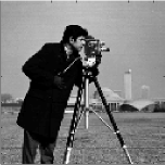
Figure 3: Example of MaxEnt Image Reconstruction (reprinted from [13]). Left: original $128\times 128$ image. Center: reconstructed from $48\times 48$ DCT coefficients. Right: MaxEnt reconstruction on $[0,1]$ with uniform prior.

III Experiments

III-A Training and Implementation

The D-PBN was trained by minimizing the average reconstruction error. The network was trained with the PBN Toolkit [15], using Python-based Theano [16] as a framework and GPU hardware. Training a D-PBN is typically one order of magnitude slower than a standard AEC. Derivatives needed for stochastic gradient training were generated by the symbolic processing of Theano. Note that solving (4) is iterative, so derivatives are based on analysis of the last iterations.

As explained in Section II-D, there is a chance that no visible data sample can be reconstructed from a given network output feature. The sampling efficiency is the probability of successful reconstruction. To increase sampling efficiency, the network can be initialized as a stacked restricted Boltzmann machine [17, 18], then trained as a standard stochastic PBN [14]. Once sampling efficiency is larger then about 0.5, training of the D-PBN can proceed as long as contributions of the failed samples are removed from the derivatives. A failed sample is detected when the error between $\hat{{\bf z}}=\gamma({\bf h})$ and ${\bf z}$ (See Fig. 1) is much larger then machine precision. During training, the sampling efficiency then rapidly approaches 1. In all the experiments we conducted, not a single failed sample was detected either for training or testing data for fully-trained D-PBN networks.

III-B Data Set

In the experiments, we used the MNIST handwritten character data set. The data consists of $28\times 28$ sample images, with dimension $N=784$. There are 6000 training samples and 1000 testing samples of each character. In order to adapt the data to any of the data ranges $\mathbb{R}^{N}$, $\mathbb{P}^{N}$, or $\mathbb{U}^{N}$, we first “gaussianified” the data by adding dither to the quantized data, then applied the inverse sigmoid function, resulting in a smooth Gaussian-like distribution in the range -10 and 10. This “gaussianified” data was then passed through a MaxEnt activation function to create the desired data range.

For multi-layer experiments, just three characters “3”, “8”, and “9” were chosen and only 500 samples of each character were used to train. This reduced computational complexity and also highlighted the generalization capability of D-PBN by reducing the training set.

III-C Single-Layer Experiments

In the 1-layer experiment, the task was to encode samples of the three MNIST characters in each of the data ranges ($\mathbb{R}$, $\mathbb{P}$, and $\mathbb{U}$) to a dimension of $M=24$ using a single linear transformation, then reconstruct the visible data. We compare the D-PBN with a restricted Boltzmann machine (RBM) [17] and a conventional auto-encoder (AEC) using the same 1-layer network. For RBM, and AEC, the same weight matrix was used for analysis and reconstruction (tied weights), although a separate scale factor (see $s$ in Figure 2) was allowed for reconstruction to account for different scaling, and separate reconstruction bias was used. For all methods, a linear output activation was assumed (i.e. no activation function). The reconstruction activation function was matched to the data range: linear for $\mathbb{R}$, TG for $\mathbb{P}$, and TED for $\mathbb{U}$ (See Table I). The auto-encoders were evaluated by subjective comparison of the reconstructed characters and quantitative comparison using reconstruction error.

Table 4 lists the mean-square reconstruction error for three network types and three data ranges. For $\mathbb{R}^{N}$, there is almost no difference between the methods, which can be explained by the fact that the conditional mean estimator is just least-squares which can be implemented by a linear transformation. Therefore, all methods can approximate the true conditional mean estimator. There is also very little difference in MSE for training and test data, a result of low network complexity and sufficient training data size.

For $\mathbb{P}^{N}$, the performance of the three methods varies significantly. Note that the input data is differently scaled for the three data ranges, which explains the large differences in MSE, but for a given data range, all three auto-encoders operated on the same data. D-PBN shows a 35% reduction in MSE compared to AEC. For $\mathbb{U}^{N}$, the performance of the three methods becomes even more varied, with D-PBN showing a factor of 2 reduction in MSE compared to AEC. One can conclude from this that the benefit of D-PBN is related to the “non-Gaussianity” of the data. In fact, for the Gaussian assumption, there is no benefit at all, and for data constrained to $[0,\;1]$, the benefit is very significant. Figure 4 shows the reconstructions for a random-sampling of ten characters. The quality of the D-PBN reconstruction is clear to see, especially for thinly drawn characters.

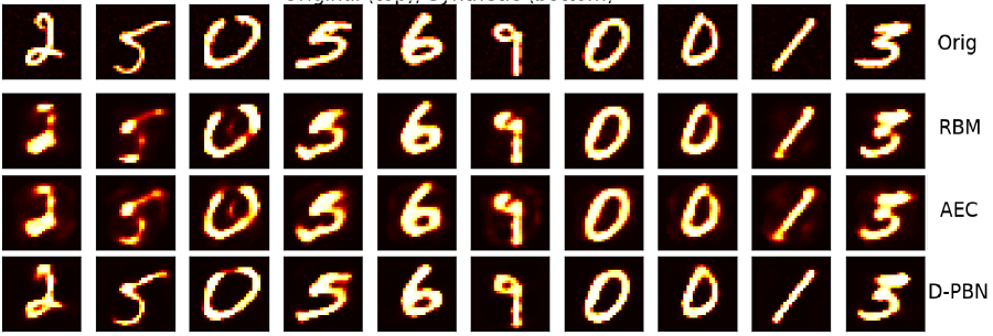
Figure 4: Reconstructed MNIST characters for 1-layer network on data range $\mathbb{U}^{N}$. All models reconstructed data from a 24-dimensional feature.

	RBM		AEC		D-PBN
Data Range $\mathbb{X}$	Train	Test	Train	Test	Train	Test
$\mathbb{R}^{N}$	3.09	3.10	3.09	3.11	3.09	3.10
$\mathbb{P}^{N}$	.896	.911	.688	.696	.5087	.5145
$\mathbb{U}^{N}$	.0172	.0173	.0152	.0154	.00725	.00734

TABLE II: Mean-square pixel reconstruction error for 1-layer networks as a function of reconstruction model and data range.

III-D Multi-Layer Experiments

Given the clear advantage of D-PBN data reconstruction in the single-layer experiment, it is relevant to ask if this holds up in a milti-layer network. After all, auto-encoders typically use non-linear activation functions in intermediate layers, with data supports of $\mathbb{U}^{N}$ for sigmoid and $\mathbb{P}^{N}$ for softplus or ReLu, and it is these data ranges where the D-PBN shows advantage.

Experiments were carried out with two and three layers. Node counts for the 2-layer network were $48,24$, and $48,24,12$ for the 3-layer networks. The layer output activation functions were chosen to correspond to the input data range, so that all layers had the same MaxEnt activation. A linear activation was used for the output of the last layer. For the multi-layer experiments, we used just a subset of the MNIST data set, as explained in Section III-B.

Instead of using RBM as a third model for comparison, we used a variational auto-encoder (VAE) which is based on a probabilistic model of the data, and has gained popularity for unsupervised learning tasks [19]. Although the VAE is technically not an auto-encoder (it is a probabilistic data model), an auto-encoder is integral to its operation. The VAE cost function employs a Kullback-Leibler divergence (KLD) term which provides good regularization effect [20, 21].

Table III lists the MSE for the three auto-encoder networks VAE, AEC, and D-PBN. Results for $\mathbb{R}^{N}$ are not included because it is a trivial case, as seen in the 1-layer results. On $\mathbb{P}^{N}$, the VAE has higher MSE than the AEC on training data, but lower on testing data, a result of regularization effect of the KLD cost function. The D-PBN is superior, for both training and testing data.

On data range $\mathbb{U}^{N}$, the VAE has higher MSE than the AEC on both training and testing data, an indication of the very high regularization effect. Recall that the VAE is primarily a statistical model. It is interesting to note that even though the D-PBN had lowest MSE on the training data, it also has better generalization performance compared to the other models. To see if additional regularization could improve the AEC, the experiment was re-run with L2 regularization, which was optimized for generalization performance. Even with optimal L2 regularization, the D-PBN performance was best. This indicates that D-PBN has a built-in regularization effect, probably due to the probabilistic basis for the model.

		VAE		AEC		D-PBN
Data Range	L2	Train	Test	Train	Test	Train	Test
$\mathbb{P}^{N}$	0	.580	.780	.500	.817	.441	.517
$\mathbb{P}^{N}$	5e-3			.552	.637
$\mathbb{U}^{N}$	0	.0236	.0254	.0104	.0112	.00773	.0087

TABLE III: Mean-square pixel reconstruction error for 2-layer networks as a function of reconstruction model and data range.

Table IV shows the results for the 3-layer experiments. The D-PBN had significantly lower reconstruction error only for $\mathbb{U}^{N}$. For $\mathbb{P}^{N}$, it was the same as the AEC.

		VAE		AEC		D-PBN
Data Range	L2	Train	Test	Train	Test	Train	Test
$\mathbb{P}^{N}$	0	.7431	1.51	.651	.867	.7153	.8665
$\mathbb{U}^{N}$	0	.216	.224	.0255	.0233	.0143	.0152

TABLE IV: Mean-square pixel reconstruction error for 3-layer networks as a function of reconstruction model and data range.

IV Discussion, Future Work, and Conclusions

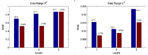
Figure 5: Summary of results by layer.

Results are summarized in Figure 5, which shows MSE as a function of layer for AEC and D-PBN. For data range $\mathbb{P}^{N}$, with data in $[0,\;\infty]$, the D-PBN results in lower MSE, but the improvement vanishes for more than 2 layers. For data range $\mathbb{U}^{N}$, with data in $[0,\;1]$, the the improvement of D-PBN is high as a factor of 2, and continues to be significant at 3 layers. This indicates that the D-PBN is preferable for auto-encoding in shallow networks and/or when data is constrained to $[0,\;1]$. The sigmoid activation, which produces data in the range $[0,\;1]$, is no longer widely-used and has been replaced by ReLU and softplus, which carry more amplitude information and are not affected by the problem of vanishing gradients. However, in light of the above results, it may be worth another look. As future work, this must be tested on other data sets, and on deeper networks.

References

- [1] L. E. Boucheron and P. L. D. Leon, “On the inversion of mel-frequency cepstral coefficients for speech enhancement applications,” IEEE Conference on Signals and Electronic Systems (ICSES08), pp. 485–488, 2008.
- [2] B. Milner and X. Shao, “Speech reconstruction from mel-frequency cepstral coefficients using a source-filter model.,” in INTERSPEECH, Citeseer, 2002.
- [3] D. Chazan, R. Hoory, G. Cohen, and M. Zibulski, “Speech reconstruction from mel frequency cepstral coefficients and pitch frequency,” in Proceedings ICASSP 2000, pp. 1299–1302, 2000.
- [4] S. J. Wernecke and L. R. D’Addario, “Maximum entropy image reconstruction,” IEEE Trans. Computers, vol. C-26, no. 4, pp. 351–364, 1977.
- [5] G. Wei and H. Zhen-Ya, “A new algorithm for maximum entropy image reconstruction,” in Proceedings of ICASSP-87, vol. 12, pp. 595–597, April 1987.
- [6] S. Kay, Fundamentals of Statisticsl Signal Processing, Estimation Theory. Prentice Hall, Upper Saddle River, New Jersey, USA, 1993.
- [7] E. T. Jaynes, “On the rationale of maximum-entropy methods,” Proceedings of IEEE, vol. 70, no. 9, pp. 939–952, 1982.
- [8] P. M. Baggenstoss, “Applications of projected belief networks (pbn),” in Proceedings of EUSIPCO 2019, (La Coruña, Spain), Sep 2019.
- [9] P. M. Baggenstoss, “A neural network based on first principles,” in ICASSP 2020, Barcelona (virtual), (Barcelona, Spain), Sep 2020.
- [10] P. M. Baggenstoss, “Applications of projected belief networks (PBN),” Proceedings of EUSIPCO, A Corunã, Spain, 2019.
- [11] P. M. Baggenstoss, “The projected belief network classifier: both generative and discriminative,” Proceedings of EUSIPCO, Amsterdam, 2020.
- [12] J. N. Kapur, Maximum Entropy Models in Science and Engineering. Wiley (Eastern), 1993.
- [13] P. M. Baggenstoss, “Uniform manifold sampling (UMS): Sampling the maximum entropy pdf,” IEEE Transactions on Signal Processing, vol. 65, pp. 2455–2470, May 2017.
- [14] P. M. Baggenstoss, “On the duality between belief networks and feed-forward neural networks,” IEEE Transactions on Neural Networks and Learning Systems, pp. 1–11, 2018.
- [15] P. Baggenstoss, “PBN Toolkit,” http://class-specific.com/pbntk.
- [16] J. Bergstra, O. Breuleux, F. Bastien, P. Lamblin, R. Pascanu, J. Turian, D. Warde-Farley, and Y. Bengio, “Theano: A cpu and gpu math expression compiler,” Proceedings of the Python for Scientific Computing Conference (SciPy), 2010.
- [17] M. Welling, M. Rosen-Zvi, and G. Hinton, “Exponential family harmoniums with an application to information retrieval,” Advances in neural information processing systems, 2004.
- [18] G. E. Hinton, S. Osindero, and Y.-W. Teh, “A fast learning algorithm for deep belief nets,” in Neural Computation 2006, 2006.
- [19] C. Doersch, “Tutorial on variational autoencoders,” arXiv preprint arXiv:1606.05908, 2016.
- [20] S. Odaibo, “Tutorial: Deriving the standard variational autoencoder (vae) loss function,” 2019.
- [21] D. J. Rezende, S. Mohamed, and D. Wierstra, “Stochastic backpropagation and approximate inference in deep generative models,” in Proceedings of the 31st International Conference on Machine Learning (E. P. Xing and T. Jebara, eds.), vol. 32 of Proceedings of Machine Learning Research, (Bejing, China), pp. 1278–1286, PMLR, 22–24 Jun 2014.