Simulating cosmological supercooling with a cold atom system II

Abstract

We perform an analysis of the supercooled state in an analogue of an early universe phase transition based on a one dimensional, two-component Bose gas with time-dependent interactions. We demonstrate that the system behaves in the same way as a thermal, relativistic Bose gas undergoing a first order phase transition. We propose a way to prepare the state of the system in the metastable phase as an analogue to supercooling in the early universe. While we show that parametric resonances in the system can be suppressed by thermal damping, we find that the theoretically estimated thermal damping in our model is too weak to suppress the resonances for realistic experimental parameters. However, we propose that experiments to investigate the effective damping rate in experiments would be worthwhile.

I Introduction

Recent experiments using (quasi-)one-dimensional Bose gases Langen et al. (2015); Erne et al. (2018); Prüfer et al. (2018) have demonstrated the potential of ultracold atom systems to be used as test-bed systems with which to study many-body quantum dynamics. Such systems are a key candidate for quantum simulators of cosmological processes Roger et al. (2016); Eckel et al. (2018).

The present work is related to simulating phase transitions in the very early universe. In some of these phase transitions, the universe would have supercooled into a metastable phase, or even into a ‘false vacuum’ state, before undergoing a first order phase transition. The ensuing violent fluctuations in density would have echoes in the present day universe in the form of signals in the cosmic microwave background Feeney et al. (2011) and in a background of gravitational waves Caprini et al. (2009); Hindmarsh et al. (2014).

The simulation of false vacuum decay in an ultracold atom experiment has already been discussed Fialko et al. (2015, 2017); Braden et al. (2018, 2019a); Billam et al. (2019). The scheme of Fialko et al. Fialko et al. (2015, 2017) uses a two-component Bose gas formed from two spin states of a spinor condensate, coupled by a time-modulated microwave field. After time-averaging, one obtains an effective description containing a metastable false vacuum state in addition to the true vacuum ground state. Within this description the relative phase between the two components behaves like a relativistic scalar field, making this an ideal system for reproducing features of high energy particle physics.

Refs. Fialko et al. (2015, 2017); Braden et al. (2018) studied the decay of the false vacuum using field-theoretical instanton techniques Coleman (1977); Callan and Coleman (1977) and numerical simulations using the truncated Wigner technique Steel et al. (1998); Blakie et al. (2008). However, Refs. Braden et al. (2018, 2019b) showed that the false vacuum state in this scheme can suffer from a parametric instability caused by the time-modulation of the system. The instability causes decay of the false vacuum state by a different mechanism than a first-order phase transition. This instability presents a challenge to experimental implementation of the scheme.

This scheme was recently extended to a finite-temperature 1D Bose gas, with temperatures in the phase-fluctuating quasi-condensate regime Billam et al. (2020), with the aim of studying thermodynamical first order phase transitions in a cold atom system. Working in the time-averaged effective description, both instanton techniques and the stochastic projected Gross–Pitaevskii equation (SPGPE) Gardiner et al. (2002); Gardiner and Davis (2003); Bradley et al. (2008); Bradley and Blakie (2014) were used to investigate the decay of a supercooled gas which has been prepared in the metastable state at low (but nonzero) temperatures. These methods showed excellent agreement in their predictions for the rate of the resulting first-order phase transition. Furthermore, the results hold out the possibility that the thermal dissipation present in the system could potentially stabilize the system against the parametric instability. However, because the time-averaged effective description was used, the mechanism of the parametric instability was explicitly removed in the model of Ref. Billam et al. (2020). To understand whether experiments could realistically observe phase transition dynamics from a supercooled metastable state using this scheme, two key questions to answer are: (i) how to prepare the ultracold atom system in the appropriate metastable state, and (ii) whether supercooled metastable states can be stabilized against the parametric instability for realistic levels of dissipation encountered in a finite-temperature Bose gas experiment.

In this paper, we address these questions using an SPGPE description of the full time-dependent system. With regard to metastable state preparation, we propose that the system is initialized first in a stable state, and then the microwave field is adjusted by a control parameter in such a way that the stable state becomes metastable. This is analagous to what happens in the early universe, where the particle fields are in a symmetric state at high temperature and a broken symmetry state at low temperature Kirzhnits and Linde (1972); Dolan and Jackiw (1974); Weinberg (1974). With regard to stabilization against the parametric instability, our theoretical analysis and numerical simulations show that thermal dissipation can stabilize the false vacuum state against the instability, allowing one to observe decay of the false vacuum state via a thermal first-order phase transition. However, for realistic experimental parameters the damping rate required for stabilization is significantly in excess of the rate predicted within the SPGPE description close to equilibrium. We discuss some of the possible caveats around taking this rate too literally in our non-equilibrium experimental scenario. We conclude that experiments measuring damping rates in non-equilibrium, quasi-1D Bose gases, would be helpful to settle the question definitively.

The remainder of the paper is structured as follows. The system is described in section II. A theoretical analysis in section III explores the parametric resonance phenomenon and demonstrates that thermal damping is able to suppress the resonance. A numerical investigation, including the initialisation stage and showing bubble nucleation, is presented in section IV. Section V gives physical values for the parameters based on a particular atomic species, and improvements to the present scenario are described in the concluding section.

II System

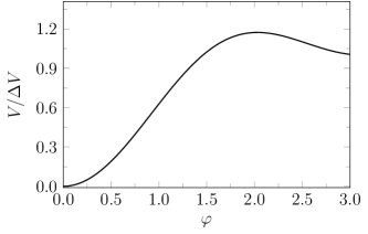
Figure 1: The field potential $V$ plotted as a function of the relative phase of the two atomic wave functions, $\varphi$. The metastable phase is at the minimum $\varphi=\pi$ and the stable phase is at the global minimum $\varphi=0$. The difference in energy density between these phases is $\Delta V$.

The system is a one-dimensional, two-component Bose gas of atoms with mass $m$. The two components are different spin states of the same species, separated in energy by an external magnetic field and coupled by a time-modulated microwave field. The Hamiltonian is given by

$$H=\int d^{n}x\left\{-{\hbar^{2}\over 2m}\psi^{\dagger}\nabla^{2}\psi+V_{\rm osc}(\psi,\psi^{\dagger})\right\}.$$ (1)

where the field operator $\psi$ has two components $\psi_{i}$, $i=1,2$. The trapping potential has been omitted, as we are interested in geometries where this is uniform across the system. The potential $V_{\rm osc}$ represents the atomic interactions,

$$V_{\rm osc}=\frac{g}{2}\sum_{i}\left(\psi_{i}^{\dagger}\psi_{i}\right)^{2}-\mu\psi^{\dagger}\psi-(\mu\epsilon^{2}+\delta\hbar\omega\cos\omega t)\,\psi^{\dagger}\sigma_{x}\psi,$$ (2)

where $\sigma_{\{x,y\}}$ are Pauli matrices. The interaction potential includes the chemical potential $\mu$, and equal intra-component $s$-wave interactions of strength $g$ between the field operators. (We assume inter-component $s$-wave interactions have been suppressed by tuning the external magnetic field.) Microwave-induced interaction terms have a constant contribution determined by a (small) dimensionless parameter $\epsilon$ and a modulation depending on another (small) parameter $\delta$. When the microwave interaction terms are switched off, the potential has a degenerate vacuum state with $\langle\psi_{1}^{\dagger}\psi_{1}\rangle=\langle\psi_{2}^{\dagger}\psi_{2}\rangle=\rho_{0}$, where the mean number density $\rho_{0}=\mu/g$. The microwave interaction terms break the degeneracy of the lowest energy state, resulting in a global minimum of the potential with $\psi_{1}=\psi_{2}$, and a saddle point at $\psi_{1}=-\psi_{2}$.

By applying a quantum mechanical averaging procedure Fialko et al. (2015, 2017), Fialko et al. arrived at an effective theory that is a candidate for describing the system on timescales longer than $2\pi/\omega$. The effective potential $V_{\rm static}$, that replaces $V_{\rm osc}$, has an extra quartic interaction,

$$V_{\rm static}=\frac{g}{2}\sum_{i}\left(\psi_{i}^{\dagger}\psi_{i}\right)^{2}-\mu\psi^{\dagger}\psi-\mu\epsilon^{2}\psi^{\dagger}\sigma_{x}\psi+\frac{g}{4}\lambda\epsilon^{2}(\psi^{\dagger}\sigma_{y}\psi)^{2},$$ (3)

where $\lambda=\sqrt{2}\delta/\epsilon$. The modulation has done its job in converting the stationary point at $\psi_{1}=-\psi_{2}$ into a local minimum in the potential when $\lambda>1$. We can illustrate this by introducing the relative phase $\varphi$ between the spin components, such that the mean field $\psi_{1}\approx\rho_{0}e^{i\varphi/2}$ and $\psi_{2}\approx\rho_{0}e^{-i\varphi/2}$, then the potential becomes

$$V_{\rm static}\approx-2\mu\epsilon^{2}-2\mu\epsilon^{2}\cos\varphi+\mu\epsilon^{2}\lambda^{2}\sin^{2}\varphi.$$ (4)

The potential has a true vacuum state at $\varphi=0$ and a false vacuum at $\varphi=\pi$, as shown in Fig. 1. The height of the potential barrier between the minima is determined by $\lambda$ and $\epsilon$, and fluctuations in the phase of the wave functions are far larger than fluctuations in the modulus when $\epsilon$ is small.

In our version of the experimental proposal, the system is initially prepared in the metastable phase at a temperature $T$. Two important parameters for the system are the healing length $\xi=\hbar/(mg\rho_{0})^{1/2}$ and the sound speed $c=\hbar/(m\xi)$. In one dimension, the physics of Bose gases critically depends also on the dimensionless interaction strength parameter, $\zeta=(\rho_{0}\xi)^{-2}$, and the temperature Kheruntsyan et al. (2003, 2005); Bouchoule et al. (2012); Henkel et al. (2017). We consider the weakly interacting case, $\zeta\ll 1$. A phase-fluctuating quasi-condensate, in which density fluctuations are suppressed, appears at temperatures below the cross-over temperature

$$T_{CO}={\hbar c\rho_{0}\over k_{B}}.$$ (5)

The gas remains degenerate up to a temperature of order $T_{D}=\zeta^{-1/2}T_{CO}>T_{CO}$. We shall show that the atomic gas will behave as a relativistic Klein-Gordon system undergoing a first order phase transition at a temperature around a few percent of $T_{CO}$.

III Theoretical discussion

We will model the spinor gas with the SPGPE for the stochastic two-component field $\psi$ and its conjugate $\overline{\psi}$. From this point in the paper, we will use the healing length $\xi$ to define the length unit, and the characteristic frequency $\omega_{0}=c/\xi$ to define the time unit. The potential is measured in units of $\hbar\omega_{0}\rho_{0}$. In this section, our considerations are independent of the projection involved in the SPGPE, so for simplicity we remove it and consider a stochastic GPE (SGPE), which in dimensionless form is

$$i\dot{\psi}=(1-i\gamma)\left(-\frac{1}{2}\nabla^{2}\psi+{\partial V\over\partial\overline{\psi}}\right)+\eta,$$ (6)

where $V$ is chosen for either the oscillating potential or the averaged potential. An SGPE of this general form is another well-established stochastic description of a finite-temperature Bose gas Stoof (1999); Stoof and Bijlsma (2001). In the oscillating case,

$$V_{\rm osc}=\frac{1}{2}\sum_{i}\left(\overline{\psi}_{i}\psi_{i}-1\right)^{2}-(\epsilon^{2}+\delta\omega\cos\omega t)\,\overline{\psi}\sigma_{x}\psi.$$ (7)

The stochastic noise term $\eta$ has a Gaussian distribution, with variance

$$\langle\eta(x,t)\overline{\eta}(x^{\prime},t^{\prime})\rangle=2\gamma T\delta(x-x^{\prime})\delta(t-t^{\prime}).$$ (8)

In one dimension, the temperature is measured in units of the cross-over temperature $T_{CO}$ defined in Eq. (5). (In $n$ dimensions, the unit of temperature is $\hbar\omega_{0}\zeta^{-1/2}/k_{B}$, where $\zeta=(\rho_{0}\xi^{n})^{-2}$ is the coupling strength.)

Parametric instability sets in for wavelengths shorter than the healing length and lying in narrow resonance bands. In this section, we will verify this assertion by linearising the SGPE and using averaging techniques. We will examine the role that friction plays in damping out the parametric resonance and restoring the behavior seen for a static potential. The fully non-linear system will be analysed numerically and compared to the time averaged system in the next section.

III.1 Simple averaging

A simple averaging procedure can be used to produce effective equations describing the system on time scales large compared to the modulation timescale. Previous discussions of time averaging in the modulated system Fialko et al. (2015, 2017) have shown that the system can be described by the effective Hamiltonian with the static potential (3), which can be further reduced to a Klein-Gordon theory. Starting from the effective Hamiltonian, in Ref. Billam et al. (2020), it was shown that the SPGPE with the static potential reduces to a stochastic, damped Klein-Gordon theory. In order to complete this picture, we show below how the SPGPE with the oscillating potential reduces to the damped Klein-Gordon theory.

A re-parameterisation of the wave functions can be used to facilitate the linearisation,

$$\psi_{1} =+e^{\chi/2}e^{\sigma/2}e^{i\varphi/2}e^{i\theta/2},$$ (9)

$$\psi_{2} =\pm e^{\chi/2}e^{-\sigma/2}e^{-i\varphi/2}e^{i\theta/2}.$$ (10)

The positive and negative signs are chosen for expansion about the true or false vacuum respectively. We assume $\gamma=O(\epsilon)$ and $\delta=O(\epsilon)$, where $\epsilon$ is the RF mixing parameter introduced in the potential (2). At leading order, the SPGPE given in Eq. (6) reduces to linear (Bogoliubov-de Gennes) equations for the four fields $\chi$, $\sigma$, $\varphi$ and $\theta$. The spatial Fourier transform of the relative phase $\varphi$ couples only to the relative density variation $\sigma$,

$$\dot{\varphi} =-(a\pm 2\delta\omega\cos\omega t)\sigma-\gamma(b\pm 2\delta\omega\cos\omega t)\varphi+\eta_{\varphi},$$ (11)

$$\dot{\sigma} =(b\pm 2\delta\omega\cos\omega t)\varphi-\gamma(a\pm 2\delta\omega\cos\omega t)\sigma+\eta_{\sigma}.$$ (12)

The noise terms $\eta_{\varphi}$ and $\eta_{\sigma}$ are independent Gaussian random fields with variance $2\gamma T$. The coefficients $a$ and $b$ are functions of the wave number $k$,

$$a =\frac{1}{2}(k^{2}+4\pm 4\epsilon^{2}),$$ (13)

$$b =\frac{1}{2}(k^{2}\pm 4\epsilon^{2}).$$ (14)

Free oscillations of the un-modulated system have frequency $2\sqrt{ab}$, leading to instability of the false vacuum for small $k$.

Eqs. (11) and (12) are analogous to those which describe the stabilisation of the inverted Kapitza pendulum Fialko et al. (2015, 2017), and we follow a similar line of analysis to find a time-averaged effective theory. We set

$$\varphi =\varphi_{0}+\varphi_{1}\cos\omega t+\varphi_{2}\sin\omega t,$$ (15)

$$\sigma =\sigma_{0}+\sigma_{1}\sin\omega t+\sigma_{2}\cos\omega t,$$ (16)

where we assume $\omega^{2}\gg ab$ and the functions $\varphi_{n}$, $\sigma_{n}$ are slowly varying compared to the oscillatory terms. Taking the coefficients of the $\sin\omega t$ and $\cos\omega t$ terms in Eqs. (11) and (12) gives

$$\varphi_{1} ={a\over\omega}\sigma_{1}={2\delta a\over\omega}(\varphi_{0}-\gamma\sigma_{0}),$$ (17)

$$\sigma_{2} =-{b\over\omega}\varphi_{2}={2\delta b\over\omega}(\sigma_{0}+\gamma\varphi_{0}).$$ (18)

After substituting these back into Eqs. (11) and (12), and taking the period averages, we arrive at equations for the slowly varying terms $\varphi_{0}$ and $\sigma_{0}$. Dropping $O(\gamma\delta^{2})$ terms, and taking the long-wavelength limit $k\ll 1$, the leading terms are

$$\dot{\varphi}_{0} =-2\sigma_{0}+\overline{\eta}_{\varphi},$$ (19)

$$\dot{\sigma}_{0} =\frac{1}{2}\omega_{k}^{2}\varphi_{0}-2\gamma\sigma_{0}+\overline{\eta}_{\sigma},$$ (20)

where $\omega_{k}^{2}=k^{2}+m_{\varphi}^{2}$ and the mass $m_{\varphi}=2\epsilon(\lambda^{2}\pm 1)^{1/2}$. By eliminating $\sigma_{0}$, we find that the system is equivalent to a damped Klein-Gordon field with noise $\eta_{\rm eff}$,

$$\ddot{\varphi}_{0}+2\gamma\dot{\varphi}_{0}+\omega_{k}^{2}\varphi_{0}=\eta_{\rm eff}.$$ (21)

The false vacuum is stable against small fluctuations provided that the mass is real, i.e. $\lambda>1$. In Ref. Billam et al. (2020), the damped Klein-Gordon system of Eqs. (19) and (20) was obtained starting from the effective Hamiltonian with a static potential, $V_{\rm static}$, and then linearising the SGPE.

If the condition that $\omega^{2}\gg ab$ is dropped, then secular terms can arise which invalidate the averaging procedure used above. In order to examine this possibility, we turn to the regime of parametric resonance.

III.2 Parametric resonances

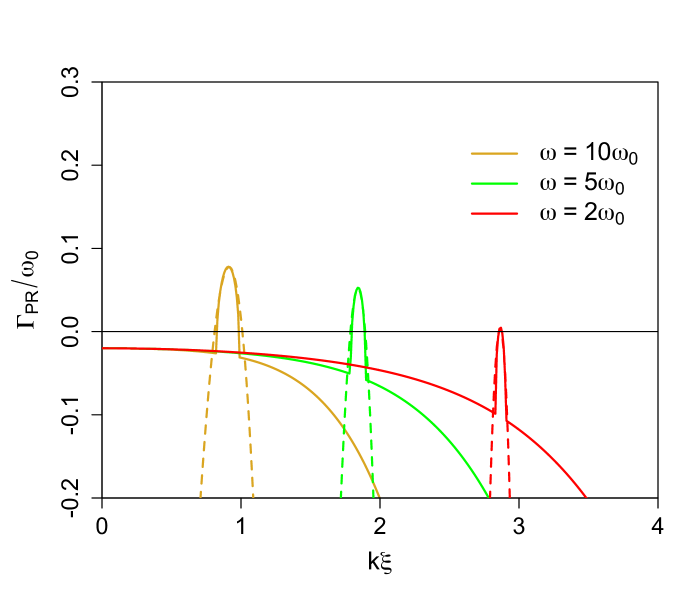
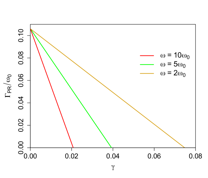
Figure 2: On the left, the growth rate $\Gamma_{PR}$ of the spatial Fourier modes, plotted as a function of wave number $k$. The microwave mixing is modulated with frequency $\omega$ and the damping is governed by the parameter $\gamma$. In this figure, $\gamma=0.02$. The resonance band approximation Eq. (29) is shown by a dotted line. On the right, the growth rate at the top of the resonant peak plotted as a function of the damping $\gamma$. In each case, the amplitude of the modulation corresponds to $\lambda=1.5$.

The system with the oscillatory potential is known to feature a parametric resonance Braden et al. (2018, 2019b) which destabilises the false vacuum when $k\sim 1$ in healing length units. The analysis in the earlier work did not take into account the effects of damping, which may act to reduce, or even remove, the parametric resonance allowing first order decay phenomena such as bubble nucleation to show up. We shall now consider parametric resonance in the unforced system with damping. The forced system with noise and parametric amplification is covered in the appendix.

Close to the first resonance, which has frequency $\omega/2$, we approximate the relative phase by

$$\varphi =A(t)\cos\left(\omega t/2\right)+B(t)\sin\left(\omega t/2\right),$$ (22)

$$\sigma =C(t)\cos\left(\omega t/2\right)+D(t)\sin\left(\omega t/2\right),$$ (23)

where $A\dots D$ are slowly varying functions of time. The time averages of (11) and (12) give equations for $A\dots D$,

$$\dot{A} =-\gamma bA-\frac{\omega}{2}B-(a+\delta\omega)C,$$ (24)

$$\dot{B} =\frac{\omega}{2}A-\gamma bB+(\delta\omega-a)D,$$ (25)

$$\dot{C} =(\delta\omega+b)A-\gamma aC-\frac{\omega}{2}D,$$ (26)

$$\dot{D} =-(\delta\omega-b)B+\frac{\omega}{2}C-\gamma aD.$$ (27)

The growth rate $\Gamma_{PR}$ of the solutions is determined by the eigenvalue of this linear system with the largest real part, $\lambda_{+}$. This depends on the wave number $k$ included in $a$ and $b$. The solutions only grow in a narrow band of $k$ values around $k=k_{b}$, where the forcing and the natural frequency coincide, i.e. $\omega^{2}=4ab$. Inserting the $a$ and $b$ from Eqs. (13) and (14), the centre of the resonance band is at

$$k_{b}^{2}=2(1+\omega^{2}/4)^{1/2}-2\mp 4\epsilon^{2}.$$ (28)

Order $\epsilon^{2}$ terms are small and we can discard them. Inside the resonance band, we let $k=k_{b}+\Delta k$, where $\Delta k$ is small. The eigenvalues of the system are parabolic in $\Delta k$,

$$\Gamma_{PR}=2\delta-\frac{1}{2}\gamma(k_{b}^{2}+2)-{(k_{b}^{2}+2)^{2}\over 4\delta(k_{b}^{2}+4)}\Delta k^{2}.$$ (29)

The growth rate in the centre of the band where $\Delta k=0$ is therefore $2\delta-(k_{b}^{2}+2)\gamma/2$. Using Eq. (28) for $k_{b}$, we see that the resonance is damped out when

$$\gamma>{4\delta\over\sqrt{4+\omega^{2}}}.$$ (30)

Since $\delta=\lambda\epsilon/\sqrt{2}$, the resonance is damped out for values of the friction $\gamma$ of order $\epsilon$, which we have taken to be small.

Figure 2 shows the growth rate of the modes with different values of the damping and modulation frequency, obtained directly from the eigenvalues of Eqs. (24) and (25) with no approximations. The underlying damping effect agrees with the damped Klein-Gordon system in Eq. (21). The resonance bands are in good agreement with the approximation (29). Higher order resonance bands have slower growth rates, and the damping is enhanced by larger $k$ values. Consequently, fluctuations in the higher resonance bands are damped out if the fluctuations in the first resonance band are damped.

IV Numerical Results

We now perform numerical simulations of the SPGPE to examine how the decay of the false vacuum proceeds in the fully non-linear system. We compare the dynamical phase transition for both the oscillating and static potential, for parameter ranges where we expect to see parametric instability, hoping to see a progression towards the first order behaviour that occurs in the static case.

In this section we use the simple growth SPGPE Gardiner et al. (2002); Gardiner and Davis (2003); Bradley et al. (2008); Blakie et al. (2008) as extended to multi-component and spinor condensates in Ref. Bradley and Blakie (2014). Including the projector, the dimensionless SPGPE reads

$$i\,d\psi=\mathcal{P}\left\{(1-i\gamma)\left(-\frac{1}{2}\nabla^{2}\psi+{\partial V\over\partial\overline{\psi}}\right)\,dt+d\eta\right\},$$ (31)

where the noise is correlated at equal times as $\langle d\eta(x,t)d\overline{\eta}(x^{\prime},t)\rangle=2\gamma T\delta(x-x^{\prime})dt$. The projection ${\cal P}$ in the SPGPE cuts off modes with wave number $k>k_{c}$, where $\hbar k_{c}=(2mk_{B}T)^{1/2}$ in physical units; this removes sparsely-populated high-momentum modes, not well-described by the classical field approximation, from the simulation Blakie et al. (2008). We take a one dimensional system with periodic boundary conditions, such as would be seen in a cold atom ring trap.

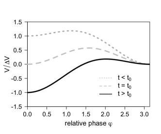
Figure 3: The potential switches from having a global minimum at $\varphi=\pi$ for $t<t_{0}$ to a local minimum when $t>t_{0}$.

An experimental protocol is required to initialise the system in a metastable phase. For the numerical simulations, we have implemented a procedure in which a minimum of the potential switches from a global to a local minimum as a control parameter, $\alpha(t)$, is changed. Conceptually, the system is loaded into the stable phase in the initial global minimum, with thermal fluctuations at temperature $T$. After a settling down period, the potential is adjusted using the control parameter so that the system enters the metastable phase.

In more detail, this initialisation step is achieved by including $\alpha(t)$ in the RF mixing terms in the interaction potential:

$$V_{\rm switch}=\frac{1}{2}\sum_{i}\left(\overline{\psi}_{i}\psi_{i}-1\right)^{2}-\left[\epsilon^{2}\cos\alpha(t)+\delta\omega\cos\omega t\right]\,\overline{\psi}\sigma_{x}\psi.$$ (32)

The RF mixing has both an oscillatory contribution with frequency $\omega$ and a slowly varying contribution with the control parameter $\alpha(t)$. Both terms are determined by the voltage input into the RF antenna. We set up $\alpha(t)$ so that

$$\alpha=\frac{\pi}{2}+\frac{\pi}{2}{\rm tanh}\left({t-t_{0}\over\tau}\right).$$ (33)

This ensures that the state with relative phase $\varphi=\pi$ is a stable minimum of the potential for $t<t_{0}$ and a metastable minimum for $t>t_{0}$, as shown in figure 3. The switching time $\tau$ is chosen to be larger than the timescale $1/\omega$, in order not to interfere with the time averaging, but chosen shorter than the bubble nucleation timescale so that the results reflect the properties of decay in the final potential rather than any transient effects.

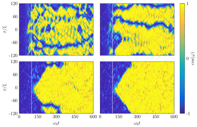
Figure 4: This series of images shows typical phase transition scenarios with different values of the damping $\gamma$ in the oscillating system. The system is prepared in a thermal state with $\varphi=\pi$ which is converted to a metastable state at $\omega_{0}t=100$ (indicated by white vertical line), with switching time $\omega_{0}\tau=5$. The top row, with $\gamma=0.005$ (left) and $\gamma=0.01$ (right), shows no evidence of bubble nucleation. The second row, with $\gamma=0.02$ (left) and $\gamma=0.03$ (right), clearly shows bubbles nucleating. By the final image, the nucleation events are indistinguishable from nucleation with a static potential. In these runs, the microwave mixing $\epsilon=0.05$, and the modulation has amplitude $\lambda=1.5$ and frequency $\omega=5\omega_{0}$.

After the potential is switched at $t=t_{0}$, our simulations show that the system nucleates false vacuum regions. Examples are shown in Fig. 4. A qualitative dependence on the damping $\gamma$ appears for the oscillating potential in the parametric resonance regime. In the low damping case, there is hardly any sign of bubble nucleation; rather, the relative phase displays strong fluctuations after a rapid growth of the instability. As the the damping is increased, the onset of bubble nucleation is a clear indication of first order behaviour. Above a certain value of $\gamma$, there is no longer any apparent difference between the oscillating potential and the static potential.

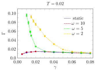
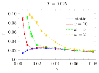
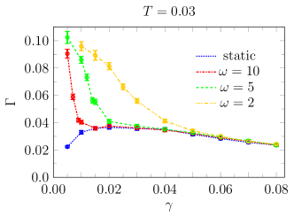
Figure 5: The decay rate is shown as a function of the friction $\gamma$ for the oscillating potential and the static potential. The rates for the oscillatory potential are larger at small $\gamma$, but agree with the rates for the static potential at larger $\gamma$. In these plots the microwave mixing is $\epsilon=0.05$ and the modulation $\lambda=1.5$. The temperatures are $T=0.02T_{CO}$, $T=0.025T_{CO}$ and $T=0.03T_{CO}$.

In order to make a quantitative comparison between the oscillating potential and the static potential, we compare the decay rate of the metastable state in the two cases. The time it takes for the phase transition is measured by observing the spatial average $\langle\cos\varphi\rangle$ to be larger than $-1+\Delta$, where $\Delta=0.9$ is chosen to be much larger than the typical fluctuations of $\langle\cos\varphi\rangle$ due to thermal noise in the system. Running many stochastic trajectories allows us to compute the probability, $P$, of remaining in the metastable state at time $t$. A fit to the exponential form $P=ae^{-\Gamma t}$ over the time intervals seen to be exhibiting exponential decay (we find this to be times late enough that $P<0.7$) yields the decay rate $\Gamma$. Error bars are estimated using a bootstrap procedure as described in Billam et al. (2019). The decay rate is plotted in Fig. 5 both for the oscillating potential, with a range of modulation frequencies, and for the static potential.

As expected from the theoretical discussion, there is a convergence in the decay rates around a value of the friction given in Eq. (30). The first order behaviour sets in when the parametric resonance is less significant than the bubble nucleation, which occurs around $\Gamma\approx\Gamma_{PR}$. There is good agreement with the theoretical predictions shown in Fig. 2.

In one of the examples, $T=0.02T_{CO}$ and $\omega=10\omega_{0}$, there is no apparent difference between the oscillating potential and the static potential. In this example, the removal of modes with $k>k_{c}$ in the SPGPE has eliminated the resonance band. This case is similar to some of the examples in Ref. Braden et al. (2019b), where there was an effective cutoff from the size of the spatial grid used in the numerical simulations. We therefore have agreement between the two sets of results for this case.

In cases close to the point where the resonance is suppressed by the cutoff we do not expect our model to be quantitatively correct, since small changes in the cutoff would have a major effect on the result. Such cutoff-dependent effects do not correspond to a physical Bose gas where there is no hard cutoff. However, this does raise the interesting question of what happens if the resonance is significantly above the cutoff wavenumber. In this regime one might expect the resonance to affect the thermal cloud more than it affects the quasi-condensate directly. Thermal cloud dynamics are outside the scope of our present SPGPE study. However, investigation of whether first-order behaviour can be seen in this regime for low damping is an interesting avenue for further work using other models that include thermal cloud dynamics Proukakis and Jackson (2008).

V Experimental realisation

We assume a cigar-shaped Bose gas tightly confined by a transverse harmonic trap of frequency $\omega_{\perp}$. Assuming a three-dimensional thermal cloud, the one-dimensional SPGPE above [Eq. (31)] with dimensionally-reduced interaction strength $g=2\hbar a_{s}\omega_{\perp}$ is a valid description provided $\hbar\omega_{\perp}\lesssim k_{\mathrm{B}}T$ Bradley et al. (2015). In principle, one should have chemical potential $\mu=\hbar\omega_{0}\ll\hbar\omega_{\perp}$. However, in practice $\omega_{0}\lesssim\omega_{\perp}$ has been found sufficient in 1D SPGPE equilibrium studies Cockburn et al. (2011); Davis et al. (2012) of quasi-1D atom-chip experiments Trebbia et al. (2006); van Amerongen et al. (2008).

As an example experimental configuration, we consider one of the experimental setups proposed by Fialko et al. Fialko et al. (2017), which is based on tuning the interactions between two Zeeman states of ${}^{41}{\rm K}$. The interactions can be tuned using a Feshbach resonance to achieve the required close-to-zero inter-component scattering length Fialko et al. (2017). Based on the intra-component scattering length $a_{s}=60$ Bohr radii, suitable experimental parameters would be $2.4\times 10^{4}$ atoms in a quasi-1D optical trap Salces-Carcoba et al. (2018) of length $218\text{\,}\mathrm{\SIUnitSymbolMicro}\mathrm{m}$ and transverse frequency $\omega_{\perp}=2\pi\times$428\text{\,}\mathrm{H}\mathrm{z}$$. The frequency $\omega_{0}$ in the suggested configuration has a value around $2\pi\times$300\text{\,}\mathrm{H}\mathrm{z}$$, and satisfies the above constraint. The interaction strength $\zeta=10^{-4}$, and the cross-over temperature $T_{CO}=$44\text{\,}\mathrm{\SIUnitSymbolMicro}\mathrm{K}$$. In this context the results in Fig. 5 correspond to temperatures of $28.8\text{\,}\mathrm{n}\mathrm{K}$, $36\text{\,}\mathrm{n}\mathrm{K}$ and $43.1\text{\,}\mathrm{n}\mathrm{K}$, where bubble nucleation should be observable. For these parameters, the bubbles in Figs. 4 and 5 are nucleating around $25$ milliseconds or so after the potential is made metastable.

Another realisation could be achieved with two Zeeman states of ${}^{7}{\rm Li}$ Fialko et al. (2017). In this case the intra-component scattering lengths of the two states are different, so that the analysis would need to be generalised. However, using the mean scattering length $a_{s}=10$ Bohr radii as a guide, a gas of $4.8\times 10^{4}$ atoms in a trap of length $102\text{\,}\mathrm{\SIUnitSymbolMicro}\mathrm{m}$ with transverse frequency $\omega_{\perp}=2\pi\times$16.1\text{\,}\mathrm{k}\mathrm{H}\mathrm{z}$$ has cross-over temperature $T_{CO}=$77.3\text{\,}\mathrm{\SIUnitSymbolMicro}\mathrm{K}$$, interaction parameter $\zeta=2.5\times 10^{-5}$, and frequency scale $\omega_{0}=2\pi\times$8.06\text{\,}\mathrm{k}\mathrm{H}\mathrm{z}$$.

While we have shown in this work that thermal damping can suppress the unwanted resonance effects in principle, the experimental value of $\gamma$ is crucial to whether or not they are actually suppressed in a given experiment. In equilibrium $\gamma$ can be predicted a priori within the SPGPE theory Bradley et al. (2008); Blakie et al. (2008), and near-equilibrium experiments have been quantitatively descibed using this a priori value of $\gamma$ Rooney et al. (2013). However, further from equilibrium SPGPE studies have typically achieved a better match to experiments by treating $\gamma$ as a free parameter that may vary significantly from the a priori value. Effective $\gamma$ values up to $\gamma=0.02$ have been employed to match experiments in this way Weiler et al. (2008); Ota et al. (2018); Liu et al. (2018).

In the experiments proposed here, bubbles nucleate from a thermal equilibrium state that has been raised to metastability by our control parameter protocol. This would appear to be a reasonably near-equilibrium scenario up until the point a bubble is nucleated and begins to grow. With the above example experimental parameters for ${}^{41}{\rm K}$, the a priori prediction for our two-component SPGPE model is $2.5\times 10^{-5}\leq\gamma\leq 4.7\times 10^{-5}$. This stated range includes the temperature difference from $0.02T_{CO}$ to $0.03T_{CO}$, and the difference between the “bare” rate and the rate adjusted by the Lerch transcendent formula of Refs.Bradley et al. (2008); Blakie et al. (2008); Bradley et al. (2015). In practice, the adjustment to the “bare” rate is small (of order 1) for these parameters. For ${}^{7}{\rm Li}$ the range is $3.4\times 10^{-6}\leq\gamma\leq 1.2\times 10^{-5}$. This suggests suppression of the resonances by thermal damping would not be achieved. However, this conclusion rests on the model we employed and the assumption that the scenario is sufficiently near-equilibrium for the a priori prediction of $\gamma$ to be relevant. As mentioned above, effective $\gamma$ values that would be sufficient to suppress some resonances have been used in previous SPGPE modelling of non-equilibrium experiments. Considerations outside our model that might affect this conclusion include 3D effects in the quasi-condensate not captured by our quasi-1D model, energy-damping terms due to scattering not captured by our simple-growth SPGPE model Rooney et al. (2012), and the previously mentioned possibility of the resonance driving dynamics of the thermal cloud not captured in the SPGPE model. These all might alter the effective $\gamma$.

VI Conclusion

We have shown using numerical modelling that an ultracold gas of atoms in two hyperfine states can act as an analogue to a relativistic system undergoing a first order phase transition, such as might have occurred in the very early universe. In particular, we have investigated whether the parametric resonance effects which previously were noted to be problematic for the systems based on an oscillatory potential might be overcome by dissipative effects. Our results suggest this is in fact unlikely for reasonable experimental parameters, based on the a priori predicted damping rates. However, uncertainty remains over whether the a priori estimate of the damping rate would apply to a non-equilibrium experiment of this type, and over effects not captured by our simple growth SPGPE model with a static thermal cloud. Experimental measurements of the effective $\gamma$ under conditions similar to those described above, performed for example by measuring experimental rates of growth towards equilibrium and comparing these to an SPGPE model Weiler et al. (2008); Ota et al. (2018); Liu et al. (2018), would be worthwhile to determine this conclusively. Further theoretical investigation of the oscillating potential setup using a description that includes thermal cloud dynamics would be an interesting avenue for further work.

However, our results from numerical modelling are in good agreement with a purely theoretical treatment of the effect of thermal damping on the parametric resonance bands. Having the system under such good theoretical control should be useful in designing future experiments. One feature which we have not been able to reproduce, and deserves further investigation, is the possibility of parametric amplification of the thermal noise.

A particularly interesting development of the present system would be to extend it to two or three dimensions. This would allow a far richer picture of interacting bubbles than in one dimension. Two dimensions would likely be optimal as the bubbles could be imaged in an experiment without being obscured by the surrounding gas. The theoretical treatment extends easily to two or three dimensions, but the main complication is the presence of boundaries. Other treatments of bubble nucleation in two dimensions have shown that the boundary can act as a site of bubble nucleation Billam et al. (2019). Both this, and extensions to metastable states of systems with a larger number of components, are avenues we hope to investigate in future work.

Appendix A Parametric amplification

In this appendix we complete the theoretical analysis of resonant effects by including the noise terms. Noise in time-periodic stochastic systems drives the phenomenon of parametric amplification, which occurs close to a resonance band even when the parametric resonance is damped out. This effect amplifies the effectiveness of the noise, increases the fluctuations in the phase and could potentially trigger early bubble nucleation.

The response of the linearised system Eqs. (11) and (12) to the noise terms can be written in terms of a matrix Green function $G_{ij}(t,t^{\prime})$, for example

$$\varphi(t)=\int_{0}^{t}dt^{\prime}\,\left\{G_{\varphi\varphi}(t,t^{\prime})\eta_{\varphi}(t^{\prime})+G_{\varphi\sigma}(t,t^{\prime})\eta_{\sigma}(t^{\prime})\right\}$$ (34)

Suppose the eigenvalues of the averaged system (24) and (25) are $\lambda_{-}$ and $\lambda_{+}$. Both of these are negative in the damped regime, and we choose $|\lambda_{+}|<|\lambda_{-}|$. The approximate solutions Eq. (22) for $\varphi$ are

$$\varphi_{+} =e^{\lambda_{+}t}\left(\cos\omega t/2-\sin\omega t/2\right),$$ (35)

$$\varphi_{-} =e^{\lambda_{-}t}\left(\cos\omega t/2+\sin\omega t/2\right).$$ (36)

Using standard Green function methods, the $\varphi\sigma$ component of the Green function to leading order in $\epsilon$ is

$$G_{\varphi\sigma}(t,t^{\prime})={\varphi_{+}(t^{\prime})\varphi_{-}(t)-\varphi_{-}(t^{\prime})\varphi_{+}(t)\over\sigma_{+}(t^{\prime})\varphi_{-}(t^{\prime})-\sigma_{-}(t^{\prime})\varphi_{+}(t^{\prime})}\theta(t-t^{\prime}),$$ (37)

where $\theta(t)$ is the Heaviside function and $\sigma_{\pm}\approx-\dot{\varphi}_{\pm}/a$ from Eq. (11).

The correlation function for the phase driven by the $\eta_{\sigma}$ noise becomes

$$\langle\varphi(k,t)\varphi^{*}(k^{\prime},t)\rangle=2\gamma T\int_{0}^{t}dt^{\prime}\,G_{\varphi\sigma}(t,t^{\prime})^{2}\delta_{kk^{\prime}},$$ (38)

where the dependence on wavenumber is implicit in the modes (37). The rapidly oscillating terms average out, and we are left with

$$\langle\varphi(k,t)\varphi^{*}(k^{\prime},t)\rangle\approx{a^{2}\gamma T\over\omega^{2}}\left({1\over|\lambda_{+}|}+{1\over|\lambda_{-}|}\right)\delta_{kk^{\prime}}.$$ (39)

At the centre of the resonance band, $\lambda_{+}$ is given by Eq. (29), and

$$\langle\varphi(k,t)\varphi^{*}(k^{\prime},t)\rangle\approx{a\gamma T\over 4b|4\delta-(2+k^{2})\gamma|}\delta_{kk^{\prime}}.$$ (40)

Thus the variance in the phase is enhanced when the denominator, $|\lambda_{+}|$, is small. However, the variance calculated here is an equilibrium value. In practice, preparation of the system in a non-equilibrium state can lead to a smaller variance initially, and the fluctuations may take a significant time to reach the equilibrium value, at a rate depending on the eigenvalue $\lambda_{-}$. This may explain why our numerical simulations show no evidence of enhanced bubble nucleation in the small $|\lambda_{+}|$ regime.

References

- Langen et al. (2015) T. Langen, S. Erne, R. Geiger, B. Rauer, T. Schweigler, M. Kuhnert, W. Rohringer, I. E. Mazets, T. Gasenzer, and J. Schmiedmayer, Science 348, 207 (2015), arXiv:1411.7185 [cond-mat.quant-gas] .
- Erne et al. (2018) S. Erne, R. Bücker, T. Gasenzer, J. Berges, and J. Schmiedmayer, Nature 563, 225 (2018), arXiv:1805.12310 [cond-mat.quant-gas] .
- Prüfer et al. (2018) M. Prüfer, P. Kunkel, H. Strobel, S. Lannig, D. Linnemann, C.-M. Schmied, J. Berges, T. Gasenzer, and M. K. Oberthaler, Nature 563, 217 (2018), arXiv:1805.11881 [cond-mat.quant-gas] .
- Roger et al. (2016) T. Roger, C. Maitland, K. Wilson, N. Westerberg, D. Vocke, E. M. Wright, and D. Faccio, Nature Communications 7, 13492 (2016), arXiv:1611.00924 [physics.optics] .
- Eckel et al. (2018) S. Eckel, A. Kumar, T. Jacobson, I. B. Spielman, and G. K. Campbell, Phys. Rev. X 8, 021021 (2018), arXiv:1710.05800 [cond-mat.quant-gas] .
- Feeney et al. (2011) S. M. Feeney, M. C. Johnson, D. J. Mortlock, and H. V. Peiris, Phys. Rev. D 84, 043507 (2011), arXiv:1012.3667 [astro-ph.CO] .
- Caprini et al. (2009) C. Caprini, R. Durrer, T. Konstandin, and G. Servant, Phys. Rev. D 79, 083519 (2009), arXiv:0901.1661 [astro-ph.CO] .
- Hindmarsh et al. (2014) M. Hindmarsh, S. J. Huber, K. Rummukainen, and D. J. Weir, Phys. Rev. Lett. 112, 041301 (2014), arXiv:1304.2433 [hep-ph] .
- Fialko et al. (2015) O. Fialko, B. Opanchuk, A. I. Sidorov, P. D. Drummond, and J. Brand, EPL (Europhysics Letters) 110, 56001 (2015), arXiv:1408.1163 [cond-mat.quant-gas] .
- Fialko et al. (2017) O. Fialko, B. Opanchuk, A. I. Sidorov, P. D. Drummond, and J. Brand, Journal of Physics B Atomic Molecular Physics 50, 024003 (2017), arXiv:1607.01460 [cond-mat.quant-gas] .
- Braden et al. (2018) J. Braden, M. C. Johnson, H. V. Peiris, and S. Weinfurtner, JHEP 07, 014 (2018), arXiv:1712.02356 [hep-th] .
- Braden et al. (2019a) J. Braden, M. C. Johnson, H. V. Peiris, A. Pontzen, and S. Weinfurtner, Phys. Rev. Lett. 123, 031601 (2019a), arXiv:1806.06069 [hep-th] .
- Billam et al. (2019) T. P. Billam, R. Gregory, F. Michel, and I. G. Moss, Phys. Rev. D 100, 065016 (2019), arXiv:1811.09169 [hep-th] .
- Coleman (1977) S. R. Coleman, Phys. Rev. D 15, 2929 (1977), [Erratum: Phys. Rev. D 16, 1248 (1977)].
- Callan and Coleman (1977) C. G. Callan and S. R. Coleman, Phys. Rev. D 16, 1762 (1977).
- Steel et al. (1998) M. J. Steel, M. K. Olsen, L. I. Plimak, P. D. Drummond, S. M. Tan, M. J. Collett, D. F. Walls, and R. Graham, Phys. Rev. A 58, 4824 (1998), arXiv:cond-mat/9807349 [cond-mat.soft] .
- Blakie et al. (2008) P. Blakie, A. Bradley, M. Davis, R. Ballagh, and C. Gardiner, Advances in Physics 57, 363 (2008), arXiv:0809.1487 [cond-mat.quant-gas] .
- Braden et al. (2019b) J. Braden, M. C. Johnson, H. V. Peiris, A. Pontzen, and S. Weinfurtner, JHEP 10, 174 (2019b), arXiv:1904.07873 [hep-th] .
- Billam et al. (2020) T. P. Billam, K. Brown, and I. G. Moss, Phys. Rev. A 102, 043324 (2020), arXiv:2006.09820 [cond-mat.quant-gas] .
- Gardiner et al. (2002) C. W. Gardiner, J. R. Anglin, and T. I. A. Fudge, Journal of Physics B: Atomic, Molecular and Optical Physics 35, 1555 (2002), arXiv:0112129 [cond-mat] .
- Gardiner and Davis (2003) C. W. Gardiner and M. J. Davis, Journal of Physics B: Atomic, Molecular and Optical Physics 36, 4731 (2003), arXiv:0308044 [cond-mat] .
- Bradley et al. (2008) A. S. Bradley, C. W. Gardiner, and M. J. Davis, Phys. Rev. A 77, 033616 (2008), arXiv:1804.04032 [cond-mat.quant-gas] .
- Bradley and Blakie (2014) A. S. Bradley and P. B. Blakie, Phys. Rev. A 90, 023631 (2014), arXiv:1406.2029 [cond-mat.quant-gas] .
- Kirzhnits and Linde (1972) D. Kirzhnits and A. Linde, Physics Letters B 42, 471 (1972).
- Dolan and Jackiw (1974) L. Dolan and R. Jackiw, Phys. Rev. D 9, 3320 (1974).
- Weinberg (1974) S. Weinberg, Phys. Rev. D 9, 3357 (1974).
- Kheruntsyan et al. (2003) K. V. Kheruntsyan, D. M. Gangardt, P. D. Drummond, and G. V. Shlyapnikov, Phys. Rev. Lett. 91, 040403 (2003), arXiv:0212153 [cond-mat.stat-mech] .
- Kheruntsyan et al. (2005) K. V. Kheruntsyan, D. M. Gangardt, P. D. Drummond, and G. V. Shlyapnikov, Phys. Rev. A 71, 053615 (2005), arXiv:0502438 [cond-mat.stat-mech] .
- Bouchoule et al. (2012) I. Bouchoule, M. Arzamasovs, K. V. Kheruntsyan, and D. M. Gangardt, Phys. Rev. A 86, 033626 (2012), arXiv:1207.4627 [cond-mat.quant-gas] .
- Henkel et al. (2017) C. Henkel, T.-O. Sauer, and N. P. Proukakis, Journal of Physics B: Atomic, Molecular and Optical Physics 50, 114002 (2017), arXiv:1701.03133 [cond-mat.quant-gas] .
- Stoof (1999) H. Stoof, Journal of Low Temperature Physics 114, 11 (1999), arXiv:9805393 [cond-mat.stat-mech] .
- Stoof and Bijlsma (2001) H. T. C. Stoof and M. J. Bijlsma, Journal of Low Temperature Physics 124, 431 (2001), arXiv:0007026 [cond-mat.stat-mech] .
- Proukakis and Jackson (2008) N. P. Proukakis and B. Jackson, J. Phys. B 41, 203002 (2008), arXiv:0810.0210 [cond-mat.other] .
- Bradley et al. (2015) A. S. Bradley, S. J. Rooney, and R. G. McDonald, Phys. Rev. A 92, 033631 (2015), arXiv:1507.02023 [cond-mat.quant-gas] .
- Cockburn et al. (2011) S. P. Cockburn, D. Gallucci, and N. P. Proukakis, Phys. Rev. A 84, 023613 (2011), arXiv:1103.2740 [cond-mat.quant-gas] .
- Davis et al. (2012) M. J. Davis, P. B. Blakie, A. H. van Amerongen, N. J. van Druten, and K. V. Kheruntsyan, Phys. Rev. A 85, 031604 (2012), arXiv:1108.3608 [cond-mat.quant-gas] .
- Trebbia et al. (2006) J.-B. Trebbia, J. Esteve, C. I. Westbrook, and I. Bouchoule, Phys. Rev. Lett. 97, 250403 (2006), arXiv:0606247 [quant-ph] .
- van Amerongen et al. (2008) A. H. van Amerongen, J. J. P. van Es, P. Wicke, K. V. Kheruntsyan, and N. J. van Druten, Phys. Rev. Lett. 100, 090402 (2008), arXiv:0709.1899 [cond-mat.other] .
- Salces-Carcoba et al. (2018) F. Salces-Carcoba, C. J. Billington, A. Putra, Y. Yue, S. Sugawa, and I. B. Spielman, New Journal of Physics 20, 113032 (2018), arXiv:1808.06933 [cond-mat.quant-gas] .
- Rooney et al. (2013) S. J. Rooney, T. W. Neely, B. P. Anderson, and A. S. Bradley, Phys. Rev. A 88, 063620 (2013), arXiv:1208.4421 [cond-mat.quant-gas] .
- Weiler et al. (2008) C. N. Weiler, T. W. Neely, D. R. Scherer, A. S. Bradley, M. J. Davis, and B. P. Anderson, Nature 455, 948 (2008), arXiv:0807.3323 [cond-mat.other] .
- Ota et al. (2018) M. Ota, F. Larcher, F. Dalfovo, L. Pitaevskii, N. P. Proukakis, and S. Stringari, Phys. Rev. Lett. 121, 145302 (2018), arXiv:1804.04032 [cond-mat.quant-gas] .
- Liu et al. (2018) I.-K. Liu, S. Donadello, G. Lamporesi, G. Ferrari, S.-C. Gou, F. Dalfovo, and N. P. Proukakis, Commun Phys 1, 24 (2018), arXiv:1712.08074 [cond-mat.quant-gas] .
- Rooney et al. (2012) S. J. Rooney, P. B. Blakie, and A. S. Bradley, Phys. Rev. A 86, 053634 (2012), arXiv:1210.0952 [cond-mat.quant-gas] .