Abstract

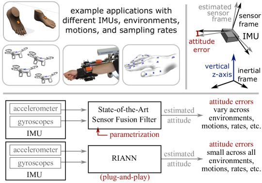
Inertial-sensor-based attitude estimation is a crucial technology in various applications, from human motion tracking to autonomous aerial and ground vehicles. Application scenarios differ in characteristics of the performed motion, presence of disturbances, and environmental conditions. Since state-of-the-art attitude estimators do not generalize well over these characteristics, their parameters must be tuned for the individual motion characteristics and circumstances. We propose RIANN, a ready-to-use, neural network-based, parameter-free, real-time-capable inertial attitude estimator, which generalizes well across different motion dynamics, environments, and sampling rates, without the need for application-specific adaptations. We gather six publicly available datasets of which we exploit two datasets for the method development and the training, and we use four datasets for evaluation of the trained estimator in three different test scenarios with varying practical relevance. Results show that RIANN outperforms state-of-the-art attitude estimation filters in the sense that it generalizes much better across a variety of motions and conditions in different applications, with different sensor hardware and different sampling frequencies. This is true even if the filters are tuned on each individual test dataset, whereas RIANN was trained on completely separate data and has never seen any of these test datasets. RIANN can be applied directly without adaptations or training and is therefore expected to enable plug-and-play solutions in numerous applications, especially when accuracy is crucial but no ground-truth data is available for tuning or when motion and disturbance characteristics are uncertain. We made RIANN publicly available.

1 1 0 https://doi.org/ RIANN—A Robust Neural Network Outperforms Attitude Estimation Filters RIANN—A Robust Neural Network Outperforms Attitude Estimation Filters Daniel Weber ^1,* , Clemens Gühmann ¹ and Thomas Seel ² Daniel Weber, Clemens Gühmann and Thomas Seel Weber, D.; Gühmann, C.; Seel, T. Correspondence: d.weber.1@tu-berlin.de

1 Introduction

As a result of rapid improvements in microelectromechanical systems technologies, miniature Inertial Measurement Units (IMUs) have become more and more lightweight and small at reasonable accuracies. They have thus entered a wide range of applications in which some form of motion tracking or analysis is required. Popular examples are found in aerospace engineering, autonomous vehicle technologies, robotics, and wearables for health and sports applications Seel et al. (2020).

To estimate the motion of an object from the raw readings of an IMU, one needs to determine the orientation of the sensor frame with respect to the vertical axis and horizontal plane, i.e., the attitude. While the attitude itself is of high interest in many applications (see e.g., Euston et al. (2008); Ding et al. (2018); Valarezo Añazco et al. (2021); Marco et al. (2018)), attitude estimation is also a crucial step in velocity and position strapdown integration since it enables the separation of gravitational acceleration and the change of velocity Woodman (2007).

It should be noted that often additional value lies in estimating the heading with respect to the local magnetic field from magnetometer readings. However, abundant research shows that the assumption of a homogeneous magnetic field is often violated Nazarahari and Rouhani (2021); De Vries et al. (2009), and a wide range of magnetometer-free methods and solutions rely on deriving attitude estimates directly from gyroscope and accelerometer readings Kok et al. (2014); Teufl et al. (2018); Lorenz et al. (2020); Eckhoff et al. (2020); Grapentin et al. (2020); Lehmann et al. (2020). This is sometimes called 6D (or 6-axis) sensor fusion, in contrast to 9D (or 9-axis) sensor fusion, which also incorporates the three-dimensional magnetometer readings. Any solution to the latter must contain a solution to the former.

1.1 The Challenge of Generalizability in Inertial Attitude Estimation

A multitude of advanced methods has been proposed for inertial attitude estimation via 6D sensor fusion. The vast majority of these methods are complementary filters or Kalman filters with various modifications Nazarahari and Rouhani (2021). All of these algorithms have parameters such as covariance matrices and filter gains that are used to adjust the filter to different measurement errors and motion characteristics. When an algorithm is applied to a given application problem, it is highly desirable to use it plug-and-play without any adaption of the mentioned parameters. However, given the wide variety of these conditions in different applications, state-of-the-art attitude estimators need to be tuned for every application to assure small errors Nazarahari and Rouhani (2021). This represents a significant lack of generalization ability across different motion characteristics, environmental conditions, and application demands. A recent comparison of ten different state-of-the-art filters on a dataset with three different rotation speeds has shown that filters with more tunable parameters have the potential for lower errors on a specific task but perform worse without a suitable parameter selection Caruso et al. (2021). For example, in a fast and jerky motion, the accelerometer must be used much more carefully than during a smooth and slow motion Laidig et al. .

It was found that the optimal parameter regions for different motion characteristics rarely overlap, that default parameterizations often yield inadequate results, and that specific tuning is critical for many experimental scenarios Caruso et al. (2021). To date, there is no attitude estimator that performs robustly well (i.e., without requiring parameter tuning) across the different motion characteristics, sensor hardware, sampling rates, and environmental conditions that appear in different application scenarios.

1.2 The Potential of Neural Networks in Inertial Attitude Estimation

The history of 70 years of AI research has shown that in many applications leveraging human understanding granted a short-term boost to performance and efficiency, but in the long-term more general approaches that require more computing resources and data often succeeded, for example in computer vision and natural language processing Rich (2019). Inspired by this observation, an alternative approach to the given attitude estimation task is to train a neural network end-to-end on the raw IMU data of a large variety of experimental datasets with ground truth measurements. Considering the success of neural networks in other system identification tasks Andersson et al. (2019); Oord et al. (2016), it seems promising to employ them for robust attitude estimation.

To date, neural networks have been used to augment conventional attitude estimation methods by classifying the type of motion Brossard et al. (2020a), compensating measurements errors Brossard et al. (2020b), or smoothing the output of the conventional filter Chiang et al. (2009); Dhahbane et al. (2021); Al-Sharman et al. (2020). In Esfahani et al. (2019, 2020) Recurrent Neural Networks (RNNs) are used end-to-end for the strapdown-integration but still require additional sensor fusion to be applicable in long-term attitude estimation tasks. All of these methods improve the estimation performance by optimizing the estimator for a specific task in contrast to making it more robust across different tasks. A first step in that direction has been taken by the authors of the current contribution in a recent conference paper Weber et al. (2020). Therein, a neural network structure with domain-specific adaptations has been developed and applied to a dataset with a wide variety of motions, demonstrating that neural networks can outperform conventional filters. However, the study was limited to a single dataset with one specific sensor and one specific sampling rate, which strongly limits the usefulness of the neural network for attitude estimation.

1.3 Contributions

The present work introduces RIANN (Robust IMU-based Attitude Neural Network), a ready-to-use, real-time capable, neural-network-based attitude estimator with no need for task- or condition-specific tuning. The main contributions are:

• We propose three domain-specific advances for neural networks in the context of inertial attitude estimation.

• We identify two methods that enable neural networks to handle different sampling rates in system identification tasks.

• We present the attitude estimation neural network RIANN, which results from these advances, and make it publicly available at Weber (2021).

• We combine six different publicly available datasets for a comprehensive evaluation of the robustness of attitude estimation methods.

• We compare RIANN with commonly used state-of-the-art attitude estimation filters in three evaluation scenarios with different degrees of practical relevance.

• We show that RIANN consistently outperforms commonly used state-of-the-art attitude estimation filters across different applications, motion characteristics, sampling rates, and sensor hardware.

2 Problem Statement

The problem that is addressed by the present work is to design an attitude estimator that processes the gyroscope and accelerometer measurements of an IMU to provide real-time estimates of the sensor’s attitude with respect to the vertical axis defined by Earth’s gravitational field. In the following, we give a precise definition of the problem and the performance metric by which any solution to that problem can be assessed.

Consider the fundamental problem of attitude estimation, in which an inertial sensor with a right-handed coordinate system $\mathcal{S}$ is rigidly attached to an object of interest. For any motion that the object of interest performs, we strive to estimate the sensor’s attitude, i.e., the orientation of the frame $\mathcal{S}$ with respect to the vertical axis. That estimation should be based on current and previous (but not future) measurement samples $\mathbf{a}(t_{k})$ and $\mathbf{g}(t_{k})$ of the three-dimensional accelerometers and gyroscopes, respectively, i.e., we consider a filtering problem and omit magnetometer readings. See Figure 1 for illustration.

Unlike many previous works, we refrain from assuming an initial rest period for filter convergence, since we deem this assumption too restrictive for a range of application scenarios. For the same reason, we assume that the inertial sensor is factory-calibrated, but no dedicated calibration of the turn-on bias has been performed. Such bias calibration algorithms typically also require static periods, which are difficult to assure and restrictive to assume in many applications. Instead, we consider the non-restrictive setting in which the estimation task is initialized during some motion with arbitrary rotation and translation characteristics, and the available gyroscope and accelerometer measurements exhibit standard noise and bias errors.

We formalize the given attitude estimation task using the mathematical notion of unit quaternions, which avoids the singularities in Euler angles. Let $\mathcal{E}$ be some inertial frame whose z-axis $\mathbf{e}_{z}=[0,0,1]^{\intercal}$ is aligned with the vertical axis, i.e., we neglect Earth’s rotation. Represent the relative orientation between $\mathcal{S}$ and $\mathcal{E}$ as a unit quaternion $\mathbf{q}$ with the components $[w,x,y,z]$ and assume that an estimate $\hat{\mathbf{q}}$ of that relative orientation $\mathbf{q}$ is provided by some attitude estimation algorithm. If $\hat{\mathbf{q}}$ correctly describes the sensor’s attitude, then $\hat{\mathbf{q}}$ equals ${\mathbf{q}}$ up to some heading rotation around the vertical axis, which implies that the rotation axis of the error quaternion

$$\mathbf{q}_{\text{err}}:= \mathbf{q}\otimes\left(\mathbf{\hat{q}}^{-1}\otimes\mathbf{q}\right)\otimes\mathbf{q}^{-1}$$ (1)

$$= \mathbf{q}\otimes\mathbf{\hat{q}}^{-1}$$ (2)

is exactly the z-axis. Note the important detail that $\mathbf{q}_{\text{err}}$ is defined and determined in $\mathcal{E}$ coordinates.

In the more general case of a non-zero attitude estimation error, a scalar measure is needed that quantifies the disagreement between the true and the estimated attitude regardless of the aforementioned heading difference. To this end, note that every error quaternion $\mathbf{q}_{\text{err}}$ can be decomposed into a heading error and an attitude error, i.e., into a rotation $\mathbf{q}_{\text{head\,err}}$ around the vertical axis and the smallest possible rotation $\mathbf{q}_{\text{att\,err}}$ around any horizontal axis. That smallest rotation angle can be determined analytically Laidig et al. at any sampling instant $t_{k}$ and for any given $\mathbf{q}_{\text{err}}(t_{k})=[w,x,y,z]$ by

$$e_{\alpha}(t_{k})=2\arccos\sqrt{w^{2}+z^{2}},$$ (3)

and it is equal to the angle between the true vertical axis ${\mathbf{q}}\otimes\mathbf{e}_{z}\otimes{\mathbf{q}}^{-1}$ and the estimated vertical axis $\hat{\mathbf{q}}\otimes\mathbf{e}_{z}\otimes\hat{\mathbf{q}}^{-1}$. We can therefore use $e_{\alpha}(t_{k})$ to correctly quantify the disagreement between the true attitude and any estimated attitude.

In the following, we consider established and novel methods that solve the given attitude estimation problem and quantify their performance by the root-mean-square of $e_{\alpha}(t_{k})$ over the duration of motion in many different non-restrictive scenarios.

Figure 1: IMUs are used in various applications to measure an object’s attitude with respect to the vertical axis. A robust attitude estimator, unlike conventional filters, performs well across the different sensor hardware, motion characteristics, environmental conditions, and sampling rates without application- or trial-specific parameter tuning. Graphic based on Weber et al. (2020); Beuchert et al. (2020)

3 Neural Network Structure and Implementation

In this section, we present the current state-of-the-art methods for common time series regression that are suitable for application to the attitude estimation task. Based thereon, we propose domain-specific advances, which lead to a neural network that will be trained and studied in Section 4.

3.1 Choice of the Neural Network Structure

When addressing the given problem by means of artificial neural networks, several different network structures might be considered. The main candidates for processing time-series data are Temporal Convolutional Networks (TCNs), Transformers, and Recurrent Neural Networks (RNNs).

TCNs are stateless feed-forward neural networks Andersson et al. (2019), which are able to model dynamic systems by processing windows of a fixed size at once instead of samples sequentially. Transformers are the current state-of-the-art architectures for natural language processing, because of their ability to process relations between two distant points in time Wolf et al. (2020).

RNNs have recurrent connections in their hidden layers, which store state information between time steps. The main advantage of this approach is that the calculation is very efficient and the state information may be stored infinitely in theory. In practice, there are limits to the number of time steps that may be performed before the state has degraded too much, because of the vanishing gradient problem Gonzalez and Yu (2018). Targeting this issue, many RNN architectures have been developed with Long Short-Term Memories and more recently Gated Recurrent Units (GRUs) Cho et al. (2014) being the most common one. They use a gating mechanism to alleviate the numerical problems, allowing for training with thousands instead of hundreds of time-steps in one mini-batch. The inherently sequential nature of RNNs limits the parallelizability of the training and especially the inference.

Previous work has shown that the RNN variant GRU outperforms TCNs in the attitude estimation task because of its ability to store state information over an indefinite amount of time Weber et al. (2020). Transformers on the other hand have similar capabilities but are less suited to real-time applications in environments with limited resources because of their large amount of required memory and computing capacity. Therefore, we use GRUs to process the sequential signal.

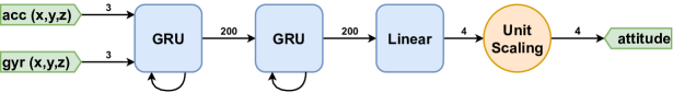
A stack of two GRU layers, which transforms the 6-dimensional IMU input $\mathbf{u}(k)$ of every sampling instant $t_{k}$ to an $N_{n}$-dimensional feature vector $\mathbf{h}(t_{k})$, with $N_{n}$ being the number of neurons per layer, has proven to be effective in attitude estimation Weber et al. (2020). To assure that the network output is a unit quaternion, the $N_{n}$-dimensional feature vector $\mathbf{h}(t_{k})$ is transformed to a four-dimensional vector $\mathbf{\hat{q}}(t_{k})$ with a Euclidean norm of 1. To this end, we use a linear layer with a weight matrix $\mathbf{W}$ for dimensional reduction and normalize the result:

$$\mathbf{\hat{q}}(t_{k})=\frac{\mathbf{W}\cdot\mathbf{h}(t_{k})}{||\mathbf{W}\cdot\mathbf{h}(t_{k})||}$$ (4)

The complete model structure is visualized in Figure 2a.

(a)  neural network structure

(b)  grouped-input neural network structure

(c)  time-aware neural network structure

Figure 2: The structure of the neural network (a); the grouped-input neural network (b) with separate layers for accelerometer and gyroscope; and the time-aware neural network (c) with the time-difference as an additional input for attitude estimation.

3.2 Neural Network Implementation with General Best Practices

We train and evaluate the neural networks with datasets that consist of multiple measured sequences of sensor and ground truth data. To avoid memorizing the same sequences, long overlapping windows get extracted from the measured sequences, so the neural network has to start at different points in time. Because of the vanishing gradient problem, RNNs can only be trained with a limited number of time steps per mini-batch. To process longer sequences in training, truncated backpropagation through time is used Tallec and Ollivier (2017). It is a method that splits sequences into a chain of shorter sequences, which are used sequentially for training with the network keeping its last hidden state between each mini-batch. To improve training stability and remove any scaling-related input signal bias, the signals are standardized to zero mean and a standard deviation of one Ioffe and Szegedy (2015). A crucial component of the training process is the optimizer. We use the current state-of-the-art combination of RAdam and Lookahead, which has proven effective in various tasks Liu et al. (2019); Zhang et al. (2019). The implementation of all adaptations in the training process has been done with the Fastai 2 API, which is based on PyTorch Howard and Gugger (2020). Parameterization of the learning rate is critical for the optimization process. We use the learning rate finder heuristic proposed in Smith (2017) for the maximum learning rate and cosine annealing for faster convergence Loshchilov and Hutter (2017).

Neural Networks have many hyperparameters that span a vast optimization space. There are two state-of-the-art hyperparameter optimization algorithms: Population Based Training (PBT) Jaderberg et al. (2017) and Asynchronous Successive Halving Algorithm (ASHA) Li et al. (2020). PBT is an evolutionary algorithm that trains a population of neural networks in parallel, relying on the survival of the fittest principle. ASHA on the other hand is an early stopping algorithm that utilizes the observation that most of the models that perform well at the final epoch also perform well early in the training process. This way the number of configurations that may be tested is increased by orders of magnitude. It has been shown that PBT performs better in reinforcement learning because it is able to learn a schedule of hyperparameters but performs worse in supervised learning Li et al. (2020). ASHA has the main advantage that it is easy to use and stable. Therefore, we optimize the neural networks in this work with ASHA.

3.3 Loss Function

For the error component of the loss function that is minimized during the training process, we use the metric $e_{\alpha}(t_{k})$ as defined in (3). Taking the mean square results in the loss function $e_{\text{MSE}}$ for a sequence of $N$ samples starting at some sampling instant $t_{k}$:

$$e_{\text{MSE}} =\frac{1}{N}\sum_{\kappa=k}^{k+N-1}e_{\alpha}(t_{\kappa})^{2}$$ (5)

As pointed out in previous work Weber et al. (2020), the gradient of the loss function grows unbounded as the optimization approaches the target argument $1$ of the $\arccos$ function, which results in numerical issues:

$$\lim\limits_{a\rightarrow 1}{\frac{\mathrm{d}\arccos(a)}{\mathrm{d}a}} =\lim\limits_{a\rightarrow 1}\frac{-1}{\sqrt{1-a^{2}}}=-\infty.$$ (6)

The solution approach Weber et al. (2020) was to replace $\arccos$ in the loss function by a linear term $1-a$ that keeps the monotonicity and correlation with the attitude. This avoids all numerical problems but leads to a discrepancy between loss function and evaluation metric Weber et al. (2020). We, therefore, propose to tackle the numerical problems directly by increasing the floating-point precision for the calculation of $e_{\alpha}(t_{k})$ to 64 bit and cutting values that are too close to 1. This results in a numerically stable and direct projection of the metric to the loss function at a negligible computational cost.

Gaps in the ground truth time series are problematic for the training process of neural networks since continuous data is needed for gradient calculation. Such gaps, however, are commonly present in motion tracking datasets due to temporary occlusion of optical markers or other disturbances of the optical reference system. Since filling the gaps compromises the integrity of the ground truth, we mask out the corresponding time intervals when generating the mini-batches.

3.4 Generalization Across Sampling Rates

In this work, the neural network is targeted to work equally well in a broad range of scenarios with different sampling rates. To allow a neural network to operate as a filter with varying sampling rates, we propose a just-in-time-resampling (JITR) network and a time-aware (TA) neural network which will be evaluated in Section 4.2.

The JITR network incorporates the idea to adapt an existing neural network that has been trained with a fixed sampling rate to the application of a broad range of sampling rates. This is achieved by resampling the input signal to the sampling rate of the neural network and doing the same in reverse with its output. This approach has the advantage of being applicable to every existing neural network. On the other hand, for every inference step, two resampling steps are required, which increases the required computation time and latency. In addition to that, more inference time steps have to be taken if the neural network has a higher sampling rate than the source signal, which increases the required computation time even more—or information is lost if the neural network has a lower sampling rate than the source signal.

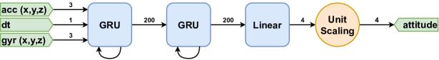
The time-aware neural network incorporates sampling rate-related information to its input, allowing it to be applied to signals of different sampling rates directly. The time difference between two samples $dt$ is used as an additional input, as visualized in Figure 2b. Since $dt$ is provided for every time step, the network is generally able to process signals with unevenly sampled data, but we leave the analysis of this case for future work. The time-aware neural network needs to be trained on data with a range of sampling rates that are expected to be used in inference time. Since neural networks are known to carry the risk of bad extrapolation beyond the range of training data, the performance of the time-aware neural network is expected to degrade outside the range of sampling rates used for training.

In both models, the input and output data have to be resampled either in the training or in the inference process. The measured acceleration and angular velocity may be resampled independently with a conventional discrete-Fourier-transformation-based method Virtanen et al. (2020). The output and reference signals are unit quaternions, which means that processing components independently generally leads to leaving the feasible set. For resampling quaternions, we thus use spherical linear interpolation Shoemake (1985).

3.5 Data Augmentation

With data augmentation, the size of the training data can be increased by using domain-specific information. With this method the generalizability of a network trained with a limited dataset may be improved, which has been demonstrated in computer vision Perez and Wang (2017) and audio processing Xiaodong Cui et al. (2015). We propose two data augmentation transformations for the attitude estimation task: the virtual IMU rotation and the induction of artificial inertial measurement errors.

For the virtual IMU rotation, we transform all accelerometer data, gyroscope data, and the ground truth attitude data of a given time interval by rotating them with a fixed randomly generated unit quaternion. If the original data was generated by moving an object with a mounted IMU, then this virtual rotation simulates the effect of attaching the IMU to the moving object in a different orientation. By this data augmentation, the network’s inference capabilities become independent of the sensor-to-object orientation, which crucially enriches any training dataset.

There are multiple kinds of errors in inertial measurement data that influence the accuracy of the attitude estimation task Zhang et al. (2020). We model the two most notable: the measurement noise and the gyroscope bias. For noise augmentation, we apply normally distributed noise with randomly generated standard deviations to each raw data sequence. The standard deviations are generated separately for the accelerometer and the gyroscope for every sequence. This also introduces varying levels of reliability of the accelerometer and the gyroscope into the training data. For the bias augmentation, an individual, randomly generated but constant offset is applied to every axis of the gyroscope measurement. The error augmentation methods add new hyperparameters to the training process, which may be picked either based on available measurement data or via a hyperparameter optimization with representative validation data, which is what we will do in Section 4.

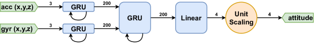
3.6 Grouped Input Channels

As an alternative method to putting all measured signals in the same first layer, we consider creating groups of signals that are processed in separate layers, which are then merged in the following one. This reduces the possible interactions between the signals, which may assist the neural network in focusing on the relevant relations between the signals. In the attitude estimation task, the first layer is split into an accelerometer and a gyroscope layer, such that the accelerometer layer may provide attitude information in slow movements and the gyroscope layer may focus on the strapdown integration during rapid movements over time. Related work employed such approaches but without analyzing the influence on the models’ performance Zheng et al. (2014); Esfahani et al. (2019), which is what we will do in Section 4.1.

4 Neural Network Optimization

In this section, we train the proposed recurrent neural network and compare different combinations of the domain-specific advances developed in Section 3 to find the best performing network configuration and hyperparameters.

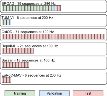
For the development of a robust network, we need a dataset with a wide spectrum of different motion characteristics. The dataset also needs to be large enough, so it can be split into training and validation data, which are used to optimize the hyperparameters and test data, which is used for performance evaluation. We meet these requirements by combining six publicly available datasets with optical ground truths from different sources and application domains. Figure 3 shows the split of the combined dataset into training, validation, and test data. The BROAD dataset is an inertial dataset with a wide variety of motion characteristics Laidig et al. . The TUM-VI dataset contains inertial and optical measurements of a handheld camera rig moving in various environments, of which we use the six room sequences because only they have an optical ground truth for the orientation over the whole sequence Schubert et al. (2018). The EuRoC-MAV dataset is composed of inertial and optical measurements on a micro aerial vehicle Burri et al. (2016). The Sassari dataset is a rich inertial dataset with measurements of several different IMUs Caruso et al. (2020). The OxIOD Dataset is an inertial dataset with multiple devices and various types of motion Chen et al. (2018). Finally, the RepoIMU dataset comprises inertial measurements from motions of a T-stick and a pendulum Szczesna et al. (2016).

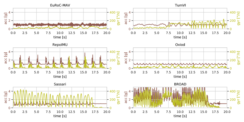
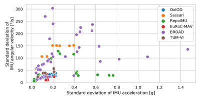
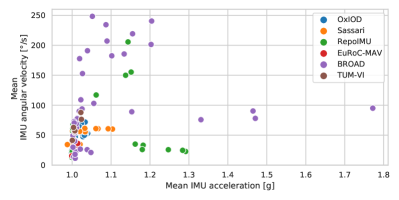
The datasets come from different applications with different motion patterns, on which a robust estimator should be able to work equally well without individual parameter tuning. Figure 4 illustrates the variety of motion characteristics in terms of one short exemplary time sequence from each dataset. The entire spectrum of motion characteristics of all sequences of all datasets is visualized in Figure 5 in terms of the mean and standard deviation of the accelerometer and gyroscope measurements. The datapoints of most datasets create narrow clusters in dataset-specific regions of the plot, which demonstrates that most applications have a specific but limited spectrum of motion characteristics. This indicates that a sufficiently rich combination of data is required for the training of a robust neural network and, likewise, for an evaluation that shows whether the network performs well across a broad range of scenarios. To preserve as many datasets as possible for the evaluation of the final network in Section 5, we decide to use only the BROAD dataset and the TUM-VI dataset for training and hyperparameter optimization in this section.

The best network configuration is determined in three steps: ablation study, sampling rate study, and network size analysis. While the ablation study quantifies the benefits of each domain-specific advance developed in Section 3, the sampling rate study identifies the best strategy for enabling the network to process data with a wide range of sampling rates. In the network size analysis, we then quantify the effect of the parameter count on the estimation accuracy and latency.

Figure 3: The dataset collection is composed of six publicly available datasets, which are split into training, validation, and test data. While the validation data is used to find the best performing network configuration and hyperparameters, the test data is reserved for the final performance evaluation in Section 5.

Figure 4: Raw signal magnitudes over time for exemplary sequences from all six datasets. Rotational and translational characteristics vary largely.

2

(a)  standard deviation of measurements

(b)  mean of measurements

Figure 5: Comparison of motion characteristics of the different datasets. Differences between datasets are considerable. The datasets BROAD, Sassari, and RepoIMU contain motions with a relatively large variety of characteristics.

2

4.1 Ablation Study

To determine the best performing network configuration, we consider all combinations of a network with/without the loss function adaptation, with/without rotation augmentation, with/without error augmentation, and with/without grouped input adaptation. This results in 16 possible network configurations. Each network configuration is trained on the training data and then applied to the validation data (cf. Figure 3) to determine the average RMSE over all validation sequences. This process is repeated five times, and the median of the five average RMSE values is used for comparison. To exclude the sampling rate question from the described procedure, all training and validation time sequences are resampled to a fixed sampling rate of 300 Hz, which is chosen higher than all source sampling rates to avoid information loss in the resampling process. We include every time sequence once without and once with an artificial turn-on gyroscope bias, which was drawn from a normal distribution with a standard deviation of 0.5$\,{}^{\circ}/\text{s}$.

The results of the described comparison show that most of the proposed advances are sequentially dependent on each other and that successive improvements can be achieved as visualized in Figure 6. A naive state-of-the-art neural network for time series processing does not achieve competitive performance when compared to conventional attitude estimation filters. Optimizing the loss function to the task-specific requirements improves the results, but the network does not generalize across different sensor-to-object orientations. The proposed data augmentation by virtual rotations solves this problem and further improves the network performance. Adding also the error augmentation further decreases the error, whereas grouping the input brings no additional benefit.

Figure 6: Ablation study of domain-specific advances, which are added successively (bottom to top). The RMSE distributions over 12 validation sequences are compared. Adaptations of the loss function and data augmentation have the largest impact on accuracy. Bold font indicates the chosen final configuration.

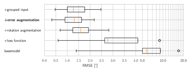
All in all, the best configuration is a state-of-the-art recurrent neural network for time series processing with an optimized loss function and data augmentation by virtual rotations and artificially induced measurement errors.

4.2 Sampling Rates Study

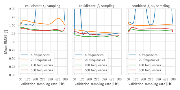
The network configuration that was identified in the previous section performs well at a single sampling rate. We now combine that network with any of the two approaches that were proposed in Section 3.4 for generalization to a broad range of sampling rates. More precisely, we first identify the best resampling strategy for the time-aware neural network and then compare it to the JITR network. The study utilizes the training and validation data (cf. Figure 3) resampled over a frequency range of 50 to 500 Hz, as detailed below. To compare different configurations, every configuration is trained five times, and as before, the median of the five average RMSE values is used for comparison.

For training the time-aware neural network, each training sequence is resampled to a certain number $N_{\text{sr}}$ of different frequencies from the given range, which effectively multiplies the number of training sequences by $N_{\text{sr}}$. To analyze the ability of the network to interpolate between sampling rate gaps, we consider training at $N_{\text{sr}}=6$, 20, 100, or 500 different sampling rates. Additionally, we consider three different strategies for drawing these different sampling rates: equidistantly over the sampling time ($t_{s}$) space (2–20 ms), equidistantly over the sampling rate ($f_{s}$) space (50–500 Hz), or both strategies combined. The performance of these different configurations is compared in terms of the average RMSE over all validation sequences resampled to any frequency between 50 and 500 Hz, as shown in Figure 7. In the given frequency range, 20 different sampling rates or less lead to sub-optimal results for all resampling strategies. With at least 100 different sampling rates, the resampling with equidistant sampling rate values yields the lowest error over the entire frequency range. Since it achieved the lowest error, we denote the time-aware neural network that was trained with 100 different equidistant sampling rates by NN-TA and disregard the other resampling configurations in the following.

Figure 7: Comparison of time-aware networks with training data that was resampled to frequencies drawn equidistantly from sampling time $t_{s}$, sampling rate $f_{s}$, or both combined. At least 100 different frequencies are required to achieve high accuracy. The $f_{s}$ space models are the most accurate across the entire frequency range.

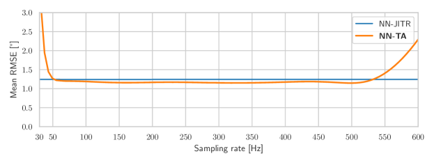
In the second step, we compare the network NN-TA with the just-in-time resampling (JITR) approach from Section 3.4. We consider the neural network that resulted from the ablation study, add a JITR of the network’s input data, and denote that combination by NN-JITR. Figure 8 visualizes the mean RMSE of NN-TA and NN-JITR over a frequency range of 30 to 600 Hz, which is broader than the range of 50 to 500 Hz on which NN-TA has been trained. NN-JITR has a stable accuracy over the complete frequency range, whereas the performance of NN-TA degrades outside of its training frequency range. However, inside that training range, NN-TA performs better than NN-JITR, which is probably due to the regularization introduced by the resampling in the training process. Considering the inference time benefits of the time-awareness approach, NN-TA seems better suited for applications in embedded systems with sampling rates within the given range of 50–500 Hz. In scenarios with completely unknown sampling rates, the JITR approach may be the better choice. For further evaluations, we consider NN-TA.

Figure 8: Comparison of the mean RMSE of NN-JITR and NN-TA over an extended sampling frequency range. NN-TA performs slightly better within the trained frequency range but fails outside. Due to just-in-time resampling, NN-JITR shows stable performance over the entire extended frequency range. Bold font indicates the chosen final configuration.

4.3 Network Size Analysis

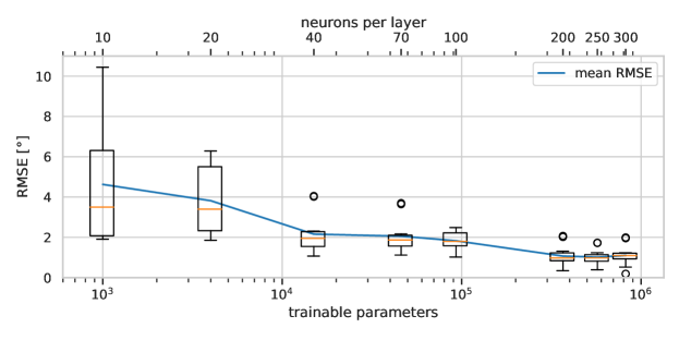
We now analyze the effect of the network size on the estimation error and required resources. To this end, NN-TA is trained with a hidden layer size in the range of 10 to 300 on the training dataset and evaluated on the validation dataset.

Figure 9 visualizes the influence of the network size on the estimation error. It also shows the exponential relationship between the number of trainable parameters and the neurons per layer. The estimation error keeps decreasing with the increase of the network size, as expected. For the decision of which network size to choose for the final network, we need to consider the trade-off between the increasing computational requirements and gains in estimation accuracy.

Figure 9: Performance of NN-TA for varying network size. Performance is quantified by box plots and the mean of the RMSE over all validation sequences. Increasing the network size leads to continuous performance improvements at the cost of an exponentially growing number of parameters.

The attitude estimation task often comes with real-time requirements that call for an algorithm that is fast enough to run on the limited hardware of an embedded system. For analysis of the required resources of NN-TA with different sizes, we evaluated the execution on a Jetson Nano noa (2019), which is a microcontroller with an integrated GPU for hardware acceleration of neural networks. On this platform the models may be executed on the CPU, representing a commonly available, fast microcontroller, or on the GPU, representing a more expensive embedded system that is specialized for the execution of neural networks. The prediction times are compared to the ones of a C implementation noa and a native Python implementation Garcia (2021) of two commonly used attitude filters Mahony et al. (2008).

Figure 10 visualizes the results of the study. The estimation latency depends on the complexity of the estimator as well as on the implementation. While a non-optimized Python implementation of Filter-A is even slower than NN-TA with over 800,000 parameters, an optimized C implementation is orders of magnitude faster. The choice of the number of parameters is essential for the inference speed of the neural network and for the required memory but has no impact on the ease of use of the final model, which will be applied plug-and-play without any change of parameter values. Considering that the error decreases significantly up to 200 neurons per layer, and considering the high performance of modern microcontrollers, we chose 200 neurons per layer for the final network, and we denote this neural network by RIANN. With 367,000 fitted parameters, RIANN has an estimation latency of 0.29 ms on the target hardware, which results in a high inference speed of 3424 Hz (fast enough for real-time applications).

Figure 10: Inference latency and mean RMSE of different neural network sizes, compared to the latency of a C and native Python implementation of popular conventional filters. On both CPU and GPU, the network RIANN with 200 neurons per layer is slightly faster than the native Python implementation.

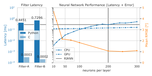
RIANN has been exported to the ONNX format to be executed with the ONNX Runtime noa (2021), which is available for a broad range of platforms and hardware. It supports an optimized C implementation for execution on the CPU of the Jetson Nano and a CUDA Version for the GPU. At low network sizes, the CPU implementation has smaller latencies than the GPU version because of the CUDA inference overhead. However, with increasing network size, the GPU latency increases only slightly because the bigger matrix multiplications can be calculated in parallel, for which the GPU is optimized.

5 Performance Evaluation

The proposed neural-network-based estimator RIANN can be considered a viable alternative to conventional attitude estimation filters only if it performs well on data from a broad range of applications with different motion characteristics, environmental conditions, sensor hardware, and sampling rates. We compare the performance of RIANN to the performance of two attitude estimation filters, which are the best performing attitude estimators with a publicly available C implementation according to a recent study of ten different estimators on a dataset with a wide variety of motions Caruso et al. (2021). We denote these filters by Filter-A Madgwick and Filter-B Mahony et al. (2008). While we will, at some point, optimize the parameters of Filter A and Filter B to individual test datasets, we will use RIANN always as it is and refrain from performing any additional training or adaptation, to realistically evaluate its performance on unseen data and unknown application scenarios.

For the intended comparison, we consider test data from several different datasets as described in Figure 3, and we consider three different scenarios that represent different levels of restrictiveness and practical relevance of the assumptions under which the network and the filters are applied to the test sequences:

• restrictive scenario: It is assumed that the sequence starts with a period of perfect rest, during which the attitude estimation can converge to an accurate estimate before the actual motion starts. Moreover, it is assumed that the turn-on bias of the gyroscopes has been removed in a preprocessing step, which requires a sufficiently long rest phase.

• partially restrictive scenario: We still assume a rest phase prior to the motion onset, but no turn-on bias correction has been conducted. We emulate this scenario by adding a random constant bias, which is drawn from a zero-mean normal distribution with a standard deviation of $0.5^{\circ}/s$, to the bias-free test sequences of the restrictive scenario.

• realistic scenario: The sensor already moves when it is turned on and the attitude estimation is started. The test sequences have the same gyroscope bias as in the partially restrictive scenario, but the initial rest periods are removed.

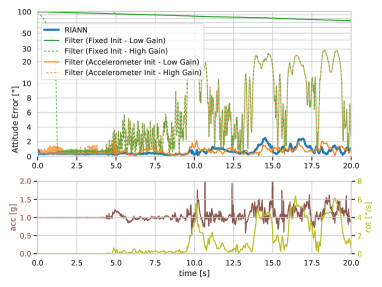
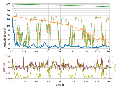
Those scenarios are chosen because these two assumptions, which make the difference between the restrictive and the realistic scenario, are crucial for the practical usability of attitude estimators in many applications, cf. Section 2. In fact, comparison between these scenarios exposes a common tuning dilemma of conventional filters, as illustrated in Figure 11 for Filter-A. A low filter gain yields a smaller long-term error, while a high gain yields more rapid initial convergence. This issue can be addressed by initializing the filter with an attitude calculated from the first accelerometer measurement rather than using a fixed initial quaternion. However, without an initial rest phase, this initialization is inaccurate, and the same dilemma occurs, cf. Figure 11b. In summary, despite accelerometer-based initialization, the low-gain filter needs several seconds up to minutes to converge but then achieves a small error, whereas the filter with a higher gain converges within seconds but exhibits larger errors in the long run. The same trade-off is observed in other filters, such as Filter-B, and similar trade-offs and dilemmas are found when balancing between fast and slow or between rotational and translational motions. It is one major goal of this study to investigate whether RIANN can overcome these limitations.

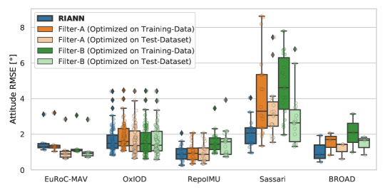
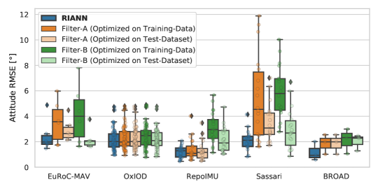
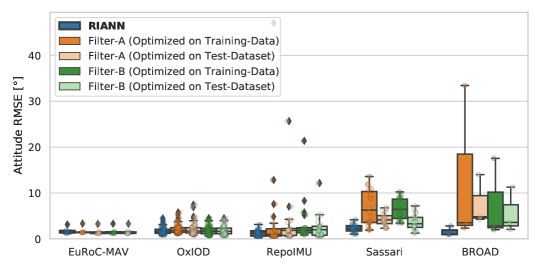
Figure 12 shows the distribution of the attitude RMSE over all test sequences, grouped by the dataset, in all three scenarios for RIANN and both conventional filters. All test sequences are evaluated with the original dataset-specific sampling frequency in which they were recorded, cf. Figure 3. The filters are evaluated in two variants: one with parameters that were numerically optimized on the training data and one with parameters that were optimized for the specific test dataset. The latter simulates the theoretical best-case in which the circumstances of the specific application are known and ground truth data is available for filter tuning. It grants the filters an advantage that the neural network does not have—RIANN was configured and trained without ever seeing any of the test data.

In the restrictive scenario, RIANN and the conventional filters perform similarly well on most datasets. However, in the more diverse and dynamic dataset Sassari, the neural network achieves consistently small errors, while the filter performance is clearly decreased, even for dataset-specific tuning. In the partially restrictive scenario with a realistic gyroscope bias, the differences become more pronounced. RIANN outperforms the conventional filters on at least two of the datasets and consistently maintains mean RMSE values at or below 2 degrees. Finally, in the realistic scenario, RIANN clearly outperforms all filter variants in all datasets except EuRoC-MAV, where the errors of all estimators stay similarly small. Especially in datasets that contain highly dynamic motions, the errors of the conventional filters increase significantly, while the neural network shows no noticeable degradation of accuracy.

The fact that RIANN performs equally well across the different IMU hardware, motion patterns, sampling rates, and environmental conditions is especially important for all practical applications in which these conditions are unknown or may change over time. In addition to the improved average performance, it is worth noting that there is not a single sequence with an RMSE of more than $4.5^{\circ}$. This means the worst-case performance of RIANN is clearly better than those of the conventional filters—even if they were tuned for the individual test dataset.

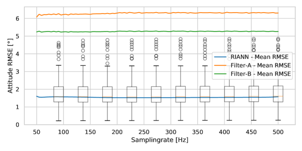
As a final test, we want to confirm that RIANN performs equally well over the whole frequency range. For this, we resample all test sequences from all datasets to many different frequencies between 50 and 500 Hz and apply RIANN to those resampled sequences, while assuming the realistic scenario. Figure 13 visualizes the mean and distribution of the RMSE values over all test sequences plotted over the frequency range. Unsurprisingly, the performance remains equally good over the entire frequency range. Not only the average but also the maximum errors of the neural network are consistently below the average errors of the conventional filters.

(a)  Start with rest

(b)  Start without rest

Figure 11: Attitude error of Filter-A and RIANN in the first 20 s of a sequence starting with rest (a) or without rest (b) with an unknown attitude. Filters exhibit a trade-off between taking a long time converging to a low error and having a larger error over the complete sequence. In sequence (a), which starts with rest, only one filter configuration provides good results. In sequence (b), which starts without rest, there is no good performing filter configuration, whereas RIANN performs similarly well as in sequence (a).

2

(a)  restrictive scenario (non-biased + initial rest)

(b)  partially restrictive scenario (biased + initial rest)

(c)  realistic scenario (biased + immediate start)

Figure 12: Comparison of RIANN with Filter-A and Filter-B, which are optimized either on the entire training data or on the specific test dataset. Across all scenarios and datasets, RIANN performs at least as good as the conventional filters and often outperforms them, especially in the realistic scenario and partially restrictive scenario.

Figure 13: RIANN’s attitude RMSE distribution (over all test sequences from all datasets) plotted over different sampling rates to which all test data is resampled. The most challenging, the realistic scenario, is considered. Performance is consistent in the filters and in RIANN, with the latter achieving consistently smaller errors.

6 Conclusions

In this work, we introduced RIANN, a ready-to-use, parameter-free, real-time-capable attitude estimator, which is based on a recurrent neural network with domain-specific advances and trained on two publically available datasets. We compared the performance of RIANN with commonly used state-of-the-art attitude filters on a combination of another four publicly available datasets from different applications.

Our results show that state-of-the-art recurrent neural networks with domain-specific adaptations perform well on the general attitude estimation task over a broad range of specific applications and conditions with no need for retraining or adjustments. RIANN even outperforms commonly used state-of-the-art attitude filters in cases, in which the filter is granted the additional advantage of parameter optimization on the target sequences. Furthermore, RIANN has shown a generally low worst-case RMSE of $4.5^{\circ}$ across all test datasets. RIANN’s performance generalizes across different hardware, sampling rates, motion characteristics, and application contexts, which were not included in the training data. This demonstrates that RIANN can be expected to perform well in applications with unknown characteristics and conditions and to yield high accuracy without the conventional need for ground truth data recording and context-specific parameter tuning.

Compared to conventional filters, RIANN requires more computational resources but can still be run in real-time applications on fast, commonly available microcontrollers without specialized hardware. The proposed domain-specific advances alter the training process but not the neural network implementation itself. This means that RIANN can be applied to a wide range of devices using the ONNX format and that platform-specific hardware acceleration capabilities can be exploited. RIANN is publicly available at Weber (2021).

Future work will be concerned with embedding RIANN into motion tracking and analysis toolchains in various applications. Furthermore, the proposed methods may be extended to the 9D inertial sensor fusion task, which incorporates magnetometer data. Another interesting aspect would be the use of neural architecture search to find the smallest optimized neural network structure that yields competitive performance for applications where the computation capacities are severely limited.

Conceptualization, methodology, validation, investigation, visualization, and writing—original draft preparation, D.W. and T.S.; writing—review and editing, D.W., C.G., and T.S.; supervision, C.G. and T.S.; software, D.W.; funding acquisition, C.G. All authors have read and agreed to the published version of the manuscript.

This work was partly funded by the German Federal Ministry of Education and Research (FKZ: 16EMO0262). We acknowledge support by the German Research Foundation and the Open Access Publication Fund of TU Berlin.

Publicly available datasets were analyzed in this study. This data can be found here: Laidig et al. ; Schubert et al. (2018); Burri et al. (2016); Caruso et al. (2020); Chen et al. (2018); Szczesna et al. (2016).

The authors declare no conflict of interest. The funder had no role in the design of the study; in the collection, analyses, or interpretation of data; in the writing of the manuscript, or in the decision to publish the results.

References

- Seel et al. (2020) Seel, T.; Kok, M.; McGinnis, R.S. Inertial Sensors—Applications and Challenges in a Nutshell. Sensors 2020, 20, 6221, doi:10.3390/s20216221.
- Euston et al. (2008) Euston, M.; Coote, P.; Mahony, R.; Kim, J.; Hamel, T. A complementary filter for attitude estimation of a fixed-wing UAV. In Proceedings of the 2008 IEEE/RSJ International Conference on Intelligent Robots and Systems, Nice, France, 22–26 September 2008; pp. 340–345, doi:10.1109/IROS.2008.4650766.
- Ding et al. (2018) Ding, W.; Xu, M.; Ma, Y.; Shi, G. Tricycle Attitude Estimation and Turn Control Based on MEMS Sensing Technology. In Proceedings of the 2018 IEEE 1st International Conference on Micro/Nano Sensors for AI, Healthcare, and Robotics (NSENS), Shenzhen, China, 5–7 December 2018; pp. 30–34, doi:10.1109/NSENS.2018.8713641.
- Valarezo Añazco et al. (2021) Valarezo Añazco, E.; Han, S.J.; Kim, K.; Lopez, P.R.; Kim, T.S.; Lee, S. Hand Gesture Recognition Using Single Patchable Six-Axis Inertial Measurement Unit via Recurrent Neural Networks. Sensors 2021, 21, 1404, doi:10.3390/s21041404.
- Marco et al. (2018) Marco, V.R.; Kalkkuhl, J.; Seel, T. Nonlinear observer with observability-based parameter adaptation for vehicle motion estimation. In Proceedings of the 18th IFAC Symposium on System Identification, (SYSID) , Stockholm, Sweden, 9–11 July 2018; pp. 60–65, doi:10.1016/j.ifacol.2018.09.091.
- Woodman (2007) Woodman, O.J. An Introduction to Inertial Navigation; Technical report; University of Cambridge, Computer Laboratory: Cambridge, UK, 2007.
- Nazarahari and Rouhani (2021) Nazarahari, M.; Rouhani, H. 40 years of sensor fusion for orientation tracking via magnetic and inertial measurement units: Methods, lessons learned, and future challenges. Inf. Fusion 2021, 68, 67–84, doi:10.1016/j.inffus.2020.10.018.
- De Vries et al. (2009) De Vries, W.; Veeger, H.; Baten, C.; Van Der Helm, F. Magnetic distortion in motion labs, implications for validating inertial magnetic sensors. Gait Posture 2009, 29, 535–541.
- Kok et al. (2014) Kok, M.; Hol, J.D.; Schön, T.B. An optimization-based approach to human body motion capture using inertial sensors. IFAC Proc. Vol. 2014, 47, 79–85.
- Teufl et al. (2018) Teufl, W.; Miezal, M.; Taetz, B.; Fröhlich, M.; Bleser, G. Validity, test-retest reliability and long-term stability of magnetometer free inertial sensor based 3D joint kinematics. Sensors 2018, 18, 1980.
- Lorenz et al. (2020) Lorenz, M.; Taetz, B.; Bleser, G. An Approach to Magnetometer-free On-body Inertial Sensors Network Alignment. In Proceedings of the IFAC World Congress, Berlin, Germany, 12–17 July 2020.
- Eckhoff et al. (2020) Eckhoff, K.; Kok, M.; Lucia, S.; Seel, T. Sparse Magnetometer-free Inertial Motion Tracking–A Condition for Observability in Double Hinge Joint Systems. In Proceedings of the 21st IFAC World Congress, Berlin, Germany, 12–17 July 2020; pp. 1–8.
- Grapentin et al. (2020) Grapentin, A.; Lehmann, D.; Zhupa, A.; Seel, T. Sparse Magnetometer-Free Real-Time Inertial Hand Motion Tracking. In Proceedings of the IEEE International Conference on Multisensor Fusion and Integration for Intelligent Systems (MFI), Karlsruhe, Germany, 14–16 September 2020; doi:10.1109/MFI49285.2020.9235262.
- Lehmann et al. (2020) Lehmann, D.; Laidig, D.; Deimel, R.; Seel, T. Magnetometer-free Inertial Motion Tracking of Arbitrary Joints with Range-of-motion Constraints. In Proceedings of the 21st IFAC World Congress, Berlin, Germany, 12–17 July 2020; pp. 1–8.
- Caruso et al. (2021) Caruso, M.; Sabatini, A.M.; Laidig, D.; Seel, T.; Knaflitz, M.; Della Croce, U.; Cereatti, A. Analysis of the Accuracy of Ten Algorithms for Orientation Estimation Using Inertial and Magnetic Sensing under Optimal Conditions: One Size Does Not Fit All. Sensors 2021, 21, 2543, doi:10.3390/s21072543.
- (16) Laidig, D.; Caruso, M.; Cereatti, A.; Seel, T. BROAD—A Benchmark for Robust Inertial Orientation Estimation. Data 2021, 6, 72, doi:10.3390/data6070072.
- Rich (2019) Rich, S. The Bitter Lesson. Available online: http://www.incompleteideas.net/IncIdeas/BitterLesson.html (accessed on 9 March 2021).
- Andersson et al. (2019) Andersson, C.; Ribeiro, A.H.; Tiels, K.; Wahlström, N.; Schön, T.B. Deep Convolutional Networks in System Identification. arXiv 2019, arXiv:1909.01730.
- Oord et al. (2016) Oord, A.V.D.; Dieleman, S.; Zen, H.; Simonyan, K.; Vinyals, O.; Graves, A.; Kalchbrenner, N.; Senior, A.; Kavukcuoglu, K. WaveNet: A Generative Model for Raw Audio. arXiv 2016, arXiv:1609.03499.
- Brossard et al. (2020a) Brossard, M.; Barrau, A.; Bonnabel, S. RINS-W: Robust Inertial Navigation System on Wheels. arXiv 2020, arXiv:1903.02210.
- Brossard et al. (2020b) Brossard, M.; Bonnabel, S.; Barrau, A. Denoising IMU Gyroscopes with Deep Learning for Open-Loop Attitude Estimation. arXiv 2020, arXiv:2002.10718.
- Chiang et al. (2009) Chiang, K.W.; Chang, H.W.; Li, C.Y.; Huang, Y.W. An Artificial Neural Network Embedded Position and Orientation Determination Algorithm for Low Cost MEMS INS/GPS Integrated Sensors. Sensors 2009, 9, 2586–2610, doi:10.3390/s90402586.
- Dhahbane et al. (2021) Dhahbane, D.; Nemra, A.; Sakhi, S. Neural Network-Based Attitude Estimation. In Artificial Intelligence and Renewables Towards an Energy Transition; Lecture Notes in Networks and Systems; Hatti, M., Ed.; Springer International Publishing: Cham, Switzerland, 2021; pp. 500–511.
- Al-Sharman et al. (2020) Al-Sharman, M.K.; Zweiri, Y.; Jaradat, M.A.K.; Al-Husari, R.; Gan, D.; Seneviratne, L.D. Deep-Learning-Based Neural Network Training for State Estimation Enhancement: Application to Attitude Estimation. IEEE Trans. Instrum. Meas. 2020, 69, 24–34, doi:\changeurlcolorblack10.1109/TIM.2019.2895495.
- Esfahani et al. (2019) Esfahani, M.A.; Wang, H.; Wu, K.; Yuan, S. AbolDeepIO: A Novel Deep Inertial Odometry Network for Autonomous Vehicles. IEEE Trans. Intell. Transp. Syst. 2019, 1–10, doi:10.1109/TITS.2019.2909064.
- Esfahani et al. (2020) Esfahani, M.A.; Wang, H.; Wu, K.; Yuan, S. OriNet: Robust 3-D Orientation Estimation With a Single Particular IMU. IEEE Robot. Autom. Lett. 2020, 5, 399–406, doi:10.1109/LRA.2019.2959507.
- Weber (2021) Weber, D. RIANN (Robust IMU-Based Attitude Neural Network). Available online: https://github.com/daniel-om-weber/riann (accessed on 15 April 2021).
- Weber et al. (2020) Weber, D.; Gühmann, C.; Seel, T. Neural Networks Versus Conventional Filters for Inertial-Sensor-based Attitude Estimation. arXiv 2020, arXiv: 2005.06897.
- Beuchert et al. (2020) Beuchert, J.; Solowjow, F.; Trimpe, S.; Seel, T. Overcoming Bandwidth Limitations in Wireless Sensor Networks by Exploitation of Cyclic Signal Patterns: An Event-triggered Learning Approach. Sensors 2020, 20, 260, doi:10.3390/s20010260.
- Wolf et al. (2020) Wolf, T.; Debut, L.; Sanh, V.; Chaumond, J.; Delangue, C.; Moi, A.; Cistac, P.; Rault, T.; Louf, R.; Funtowicz, M.; et al. HuggingFace’s Transformers: State-of-the-art Natural Language Processing. arXiv 2020, arXiv: 1910.03771.
- Gonzalez and Yu (2018) Gonzalez, J.; Yu, W. Non-linear system modeling using LSTM neural networks. IFAC-PapersOnLine 2018, 51, 485–489, doi:10.1016/j.ifacol.2018.07.326.
- Cho et al. (2014) Cho, K.; van Merrienboer, B.; Bahdanau, D.; Bengio, Y. On the Properties of Neural Machine Translation: Encoder-Decoder Approaches. arXiv 2014, arXiv:1409.1259.
- Tallec and Ollivier (2017) Tallec, C.; Ollivier, Y. Unbiasing Truncated Backpropagation Through Time. arXiv 2017, arXiv:1705.08209
- Ioffe and Szegedy (2015) Ioffe, S.; Szegedy, C. Batch Normalization: Accelerating Deep Network Training by Reducing Internal Covariate Shift. arXiv 2015, arXiv:1502.03167.
- Liu et al. (2019) Liu, L.; Jiang, H.; He, P.; Chen, W.; Liu, X.; Gao, J.; Han, J. On the Variance of the Adaptive Learning Rate and Beyond. arXiv 2019, arXiv:1908.03265.
- Zhang et al. (2019) Zhang, M.R.; Lucas, J.; Hinton, G.; Ba, J. Lookahead Optimizer: K steps forward, 1 step back. arXiv 2019, arXiv:1907.08610.
- Howard and Gugger (2020) Howard, J.; Gugger, S. Fastai: A Layered API for Deep Learning. Information 2020, 11, 108, doi:10.3390/info11020108.
- Smith (2017) Smith, L.N. Cyclical Learning Rates for Training Neural Networks. arXiv 2017, arXiv:1506.01186.
- Loshchilov and Hutter (2017) Loshchilov, I.; Hutter, F. SGDR: Stochastic Gradient Descent with Warm Restarts. arXiv 2017, arXiv:1608.03983.
- Jaderberg et al. (2017) Jaderberg, M.; Dalibard, V.; Osindero, S.; Czarnecki, W.M.; Donahue, J.; Razavi, A.; Vinyals, O.; Green, T.; Dunning, I.; Simonyan, K.; et al. Population Based Training of Neural Networks. arXiv 2017, arXiv:1711.09846.
- Li et al. (2020) Li, L.; Jamieson, K.; Rostamizadeh, A.; Gonina, E.; Hardt, M.; Recht, B.; Talwalkar, A. A System for Massively Parallel Hyperparameter Tuning. arXiv 2020, arXiv:1810.05934.
- Virtanen et al. (2020) Virtanen, P.; Gommers, R.; Oliphant, T.E.; Haberland, M.; Reddy, T.; Cournapeau, D.; Burovski, E.; Peterson, P.; Weckesser, W.; Bright, J.; et al. SciPy 1.0: Fundamental Algorithms for Scientific Computing in Python. Nat. Methods 2020, 17, 261–272, doi:10.1038/s41592-019-0686-2.
- Shoemake (1985) Shoemake, K. Animating rotation with quaternion curves. In Proceedings of the 12th Annual Conference on Computer Graphics and Interactive Techniques; SIGGRAPH ’85; Association for Computing Machinery: New York, NY, USA, 1985; pp. 245–254, doi:10.1145/325334.325242.
- Perez and Wang (2017) Perez, L.; Wang, J. The Effectiveness of Data Augmentation in Image Classification using Deep Learning. arXiv 2017, arXiv:1712.04621.
- Xiaodong Cui et al. (2015) Xiaodong Cui.; Goel, V.; Kingsbury, B. Data Augmentation for Deep Neural Network Acoustic Modeling. IEEE/ACM Trans. Audio Speech Lang. Process. 2015, 23, 1469–1477, doi:10.1109/TASLP.2015.2438544.
- Zhang et al. (2020) Zhang, Q.; Niu, X.; Shi, C. Impact Assessment of Various IMU Error Sources on the Relative Accuracy of the GNSS/INS Systems. IEEE Sen. J. 2020, 20, 5026–5038, doi:10.1109/JSEN.2020.2966379.
- Zheng et al. (2014) Zheng, Y.; Liu, Q.; Chen, E.; Ge, Y.; Zhao, J.L. Time Series Classification Using Multi-Channels Deep Convolutional Neural Networks. In Web-Age Information Management; Springer International Publishing: Cham, Switzerland, 2014; Volume 8485, pp. 298–310.
- Schubert et al. (2018) Schubert, D.; Goll, T.; Demmel, N.; Usenko, V.; Stückler, J.; Cremers, D. The TUM VI Benchmark for Evaluating Visual-Inertial Odometry. In Proceedings of the 2018 IEEE/RSJ International Conference on Intelligent Robots and Systems (IROS), Madrid, Spain, 1–5 October 2018; pp. 1680–1687. doi:\changeurlcolorblack10.1109/IROS.2018.8593419.
- Burri et al. (2016) Burri, M.; Nikolic, J.; Gohl, P.; Schneider, T.; Rehder, J.; Omari, S.; Achtelik, M.W.; Siegwart, R. The EuRoC micro aerial vehicle datasets. Int. J. Robot. Res. 2016, 35, 1157–1163, doi:\changeurlcolorblack10.1177/0278364915620033.
- Caruso et al. (2020) Caruso, M.; Cereatti, A.; Croce, U.D. mimu_optical_sassari_dataset; type: Dataset; IEEE: 2020; doi:\changeurlcolorblack10.21227/b23b-rx94.
- Chen et al. (2018) Chen, C.; Zhao, P.; Lu, C.X.; Wang, W.; Markham, A.; Trigoni, N. OxIOD: The Dataset for Deep Inertial Odometry. arXiv 2018, arXiv: 1809.07491.
- Szczesna et al. (2016) Szczesna, A.; Skurowski, P.; Pruszowski, P.; Peszor, D.; Paszkuta, M.; Wojciechowski, K. Reference Data Set for Accuracy Evaluation of Orientation Estimation Algorithms for Inertial Motion Capture Systems. In Computer Vision and Graphics; Lecture Notes in Computer Science; Chmielewski, L.J., Datta, A., Kozera, R., Wojciechowski, K., Eds.; Springer International Publishing: Cham, Switzerland, 2016; pp. 509–520.
- noa (2019) Jetson Nano Developer Kit. Available online: https://developer.nvidia.com/embedded/jetson-nano-developer-kit (accessed on 7 January 2021).
- (54) Open Source IMU and AHRS Algorithms—x-io Technologies. Available online: https://x-io.co.uk/open-source-imu-and-ahrs-algorithms/ (accessed on 28 May 2020).
- Garcia (2021) Garcia, M. Mayitzin/ahrs. Available online: https://github.com/Mayitzin/ahrs (accessed on 7 January 2021).
- Mahony et al. (2008) Mahony, R.; Hamel, T.; Pflimlin, J.M. Nonlinear Complementary Filters on the Special Orthogonal Group. IEEE Trans. Autom. Control 2008, 53, 1203–1217, doi:\changeurlcolorblack10.1109/TAC.2008.923738.
- noa (2021) ONNX Runtime: Cross-Platform, High Performance ML Inferencing and Training Accelerator. Available online: https://github.com/microsoft/onnxruntime (accessed on 10 February 2021)
- (58) Madgwick, S. An efficient orientation filter for inertial and inertial/magnetic sensor arrays. Report x-io and University of Bristol (UK) 2010 113–18