Conditional Independence for Pretext Task Selection
in Self-Supervised Speech Representation Learning

Abstract

Through solving pretext tasks, self-supervised learning (SSL) leverages unlabeled data to extract useful latent representations replacing traditional input features in the downstream task. A common pretext task consists in pretraining a SSL model on pseudo-labels derived from the original signal. This technique is particularly relevant for speech data where various meaningful signal processing features may serve as pseudo-labels. However, the process of selecting pseudo-labels, for speech or other types of data, remains mostly unexplored and currently relies on observing the results on the final downstream task. Nevertheless, this methodology is not sustainable at scale due to substantial computational (hence carbon) costs. Thus, this paper introduces a practical and theoretical framework to select relevant pseudo-labels with respect to a given downstream task. More precisely, we propose a functional estimator of the pseudo-label utility grounded in the conditional independence theory, which does not require any training. The experiments conducted on speaker recognition and automatic speech recognition validate our estimator, showing a significant correlation between the performance observed on the downstream task and the utility estimates obtained with our approach, facilitating the prospection of relevant pseudo-labels for self-supervised speech representation learning.

Index Terms: Self-Supervised Learning, Speech Representation Learning.

1 Introduction

Self-supervised learning (SSL) methods usually solve pretext tasks to learn useful representations, taking advantage of the available unlabeled data, whether it is text, images[1] or audio samples [2], for better performance on downstream tasks. Thus, this approach helps improving the results obtained on the considered task without relying on costly and sometimes imprecise manual annotations.

For instance, SSL models have recently been proposed to benefit from large amounts of unlabeled speech data, leading to state-of-the-art results in various speech processing tasks such as automatic speech recognition (ASR) or speech enhancement [3]. Various paradigms have thus been introduced including: predictive coding [4, 5, 6, 7], pseudo-label learning [8, 9], auto-encoding techniques [10, 11], generative modelling [12] or contrastive learning [13, 14].

Pretext tasks may be defined through a choice of pretext labels, hereafter referred to as pseudo-labels. The automatic generation of pseudo-labels is a common technique to conceive SSL models in many application domains such as computer vision [15], music processing [16] and speech processing [8, 17]. In the latter scenario, examples of pseudo-labels include, but are not limited to, pitch estimators, energy-based features, voicing state… As a matter of fact, decades of research in signal processing offer a wide range of potential features to be considered as pseudo-labels.

However, the process of selecting the most relevant signal features among the ones present in the speech processing literature is still essentially driven by intuition or empirical validation. Empirical assessment implies a heavy computational load due to a large number of required pretraining and fine-tuning steps. This results in a substantial carbon footprint and may lead to intractability issues. In this work, we aim to provide a clear procedure for a theoretically motivated and efficient pseudo-label selection. This is achieved by introducing a function that estimates the utility of considering a given pseudo-label.

Despite few recent works on the theory of contrastive learning [18, 19, 20, 21] the literature on the theoretical foundations of pseudo-label-based SSL remains extremely scarce. Lee and al.[20] proposed a novel approach building a link between the downstream-task performance and the conditional independence (CI) between a pseudo-label and the training samples given the downstream labels. However, their experiments are not related to speech and are restricted to pseudo-labels with an enforced strict conditional independence which is not the case of traditional speech features. On the other hand, numerous pseudo-labels have been empirically tested to generate useful latent speech representations [8]. Pascual and al.[8] introduced a novel SSL method for speech referred to as PASE alongside with a thorough empirical ablation study on the considered pseudo-labels highlighting the most influential ones. A similar study has been done on music data for instrument recognition by Hung and al.[16]. Nevertheless, neither works provide a prior quantitative motivation to justify the pseudo-labels selection that was thus potentially performed with grid or random searches. In short, and to the best of our knowledge, explaining and motivating the selection process of pseudo-labels remain open research questions for SSL on speech data. Therefore, the main contributions of our work are threefold:

1. Propose a method to compute an estimate of the conditional independence between the pretext task and the downstream speech samples given the downstream label.

2. Show that this estimate predicts well the utility of a given pseudo-label for a given downstream task, as it correlates highly with the downstream performance on two tasks: ASR (TIMIT) and speaker recognition (VoxCeleb).

3. Release the code base developed with SpeechBrain [22] for replication and to encourage further investigations.

The conducted experiments demonstrate that the proposed method allows a more intelligent, i.e. better informed, pretext task selection in self-supervised learning settings.

2 Conditional Independence Estimation

This section details the computation of the conditional independence estimate that we propose as a candidate for the measure of a pseudo-label utility. First, we motivate this choice with a precise description of the theoretical background. Then, we describe the computation steps.

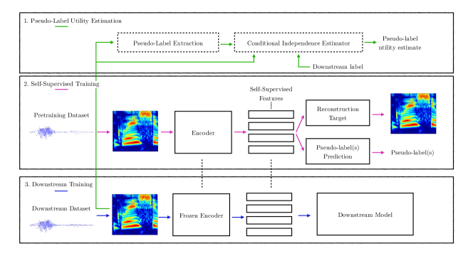
Figure 1: Illustration of the entire training pipeline including estimation, SSL and the downstream parts. The three steps are depicted: 1. estimate the pseudo-label utility; 2. SSL training with the candidate pseudo-label; 3. Train on the downstream task with the pretrained SSL model. The candidate pseudo-label is selected among various candidates based on its conditional independence score.

Let $X$, $Y$ and $Z$ be, respectively, the downstream data points, the downstream labels and the pseudo-labels which we decide to learn to predict. Let also $\mathcal{C}$ be the set of possible downstream classes. As an example, if we consider speaker recognition as a downstream task, $X$ would be the speech samples, $Y$ the speaker IDs, $\mathcal{C}$ the set of unique speaker IDs, and $Z$ a generated signal feature, such as the fundamental frequency. Let $X=(x_{i})_{i\in\{0,\ldots,M\}}$ with $M$ being the cardinal of $X$. Each $x_{i}$ is a speech sample, represented as a Mel band spectrogram. Every sample $x_{i}$ has a corresponding downstream label $y_{i}$ and an automatically generated pseudo-label $z_{i}$. In the considered cases, $y_{i}$ is always discrete, whether it is the speaker ID for speaker recognition or the phone for ASR. To every $x_{i}$, corresponds one value $z_{i}$, which is the mean of the framewise pseudo-label values.

As stated above, Lee and al.[20] linked the utility of a pseudo-label ($Z$) to the conditional independence between $Z$ and $X$ given $Y$. In other terms, given the labels $Y$, we want to quantify how much we can possibly predict the pseudo-labels $Z$ without knowing much about $X$. In this work, the authors demonstrated that under certain assumptions, the downstream classifier error was bounded by a function of the downstream training set size, and a measure of the conditional dependence. More precisely, the main theorem shows that the bounding function decreases linearly with the downstream-task dataset size ($M$) and quadratically with the conditional independence, thus making conditional independence a potential good estimator of pseudo-label utility. The principal issue with conditional independence is the difficulty of computing good estimates of this quantity on realistic data. For our measure, we choose to rely on a kernel-based independence criterion: the Hilbert Schmidt Independence Criterion (HSIC) [23]. HSIC has already been proven successful for textual data in testing statistical dependence between translated sentences[23]. Our choice is motivated by the fact that kernel-based techniques facilitate handling multivariate and complex data, as the estimation then boils down to the computation of a similarity measure between speech samples.

Here are the steps to compute our CI estimate of a pseudo-label $Z$ for a downstream task $(X,Y)$, inspired by [23], with further details below:

1. Regroup the samples $X$ by the downstream classes $\mathcal{C}$.

2. Embed the speech samples $X$ into fixed-size representations.

3. Compute for every downstream class $c\in\mathcal{C}$, the kernel matrices $K_{c}$ and $L_{c}$ containing the similarity measures for the speech samples, and the pseudo-labels, respectively.

4. Compute the independence test for every split group using $K_{c}$ and $L_{c}$, and aggregate the estimations.

We start by splitting the speech samples according to the downstream classes. To obtain the similarity matrices, the second step aims to compute fixed-size embeddings for the speech samples. We wanted to avoid any training for this phase, so we chose the gaussian downsampling method [24] detailed thereafter. After the Mel spectrogram extraction, a speech sample becomes a sequence of $L$ input feature vectors of dimension $D$. The goal is, for varying $L$, to obtain fixed size embeddings of size $N\times D$, with $N$ a fixed hyper-parameter for all the samples. To do so, the sequence is divided into $N$ parts. In each part, we compute a Gaussian average of the input frames around the center of the considered part with the standard deviation $\sigma_{gd}$ being another hyper-parameter. This leads for any sample to a $N\times D$ tensor without any training procedure.

Therefore for two speech samples $x_{i}$ and $x_{j}$, holding two pseudo-label values $z_{i}$ and $z_{j}$, the coefficients of our kernel similarity matrices are:

$$\begin{split}K_{ij}&=K(x_{i},x_{j})=cos(GD(x_{i}),GD(x_{j})),\\ L_{ij}&=RBF(z_{i},z_{j}),\end{split}$$ (1)

with $GD(.)$ the Gaussian Downsampling function, $cos(.,.)$ the cosine similarity, and $RBF(.,.)$ the Radial Basis Function kernel defined as:

$$\begin{split}cos(x,x^{\prime})&=\frac{trace(x^{T}x^{\prime})}{||x||.||x^{\prime}||},\\ RBF(x,x^{\prime})&=exp(-\frac{||x-x^{\prime}||^{2}}{2\sigma^{2}}),\end{split}$$ (2)

with $\sigma$ being the width of the RBF kernel and $trace(.)$ being the sum of elements on the main diagonal.

For each group of samples sharing the same downstream class $c\in C$, we compute the matrices $K_{c}$ and $L_{c}$. $K_{c}$ and $L_{c}$ correspond to the definitions above, but restricted to the points with $c$ as a downstream label. For each downstream class $c$, and as in [23] the HSIC value is:

$$HSIC_{c}(X,Z)=\frac{1}{n_{c}^{2}}trace(K_{c}H_{c}L_{c}H_{c}),$$ (3)

with $H_{c}=I_{n_{c}}-\frac{1}{n_{c}}1_{n_{c}}1_{n_{c}}^{T}$, $n_{c}$ being the number of points with downstream label $c$ and $1_{n_{c}}$ a vector of ones of size $n_{c}\times 1$.

The HSIC value is used to characterise the independence of two variables. This value corresponds to the Hilbert norm of their cross-covariance matrix. Intuitively, the HSIC value is high if samples similar in $K$ are similar in $L$. Therefore, the lower this value is, the more independent the two arguments of HSIC are. We enforce the condition on $Y$ by splitting by groups of points sharing the same downstream label.

The final value for a given pseudo label and a downstream task is a weighted mean taking into account the number of samples per downstream class. So with $M$ being the total number of points, and $n_{c}$ being the number of points having $c$ as their downstream label:

$$HSIC(X,Z|Y)=\frac{1}{M}\sum_{c\in\mathcal{C}}HSIC_{c}(X,Z)\times n_{c}.$$ (4)

3 Datasets and Experimental Setup

This sections details the experiments validating the CI measure described above. The estimator is evaluated on two speech tasks that involve different aspects of the audio signal: automatic speech recognition (TIMIT) and speaker recognition (VoxCeleb). Thus, three different datasets are used in this work, one per downstream task considered and a common one for the self-supervised pretraining (Common Voice). CI is computed on both tasks for a list of pseudo-labels, mainly related to prosody and aggregates of spectral descriptors, given in Table 1. These features are extracted using the OpenSmile library [25]. They have been chosen among the features described in the feature selection literature for various speech tasks.

Table 1: Candidate speech pseudo-labels and descriptions.

Feature	Description
Loudness	Intensity & approx. loudness
F0	Fundamental Frequency
Voicing	Voicing Decision
Alpha Ratio [26]	Ratio of spectrum intensity % 1000 Hz
Zero Crossing Rate	Zero crossing number per frame
RastaSpec L1Norm	L1 Norm of Rasta Spectrum [27]
log HNR [28]	log of Harmonicity to Noise Ratio

3.1 Datasets

The train set of the English Common Voice dataset (version $6.1$) [29] is used for SSL pretraining ($900$ hours). Common Voice is a collection of speech utterances from worldwide users recording themselves from their own devices. Hence, the closeness to natural settings makes it a suitable choice for self-supervised learning. We remove from Common Voice the sentences lasting more than $10$ seconds, as they often contain long silence parts due to open microphones.

VoxCeleb1 [30] is used for the speaker recognition task. The training set contains $148,642$ utterances from $1251$ different speakers. To compute the conditional independence estimates, we restricted ourselves, for tractability issues, to the utterances of $50$ different speakers (the detailed list is given in the released repository).

TIMIT [31] is considered for the ASR task. It is composed of a standard $462$-speakers training set, a $50$-speakers development set and a core test set of $192$ sentences for a total of $5$ hours of clean speech. For the CI estimation, and to get discrete labels to split on, we cut the sentences at the phone level, using the official transcripts.

3.2 Self-supervised training

Based on previous work conclusions [9, 14], apart from the pseudo-label to be tested, our self-supervised model learns to reconstruct the input Mel spectrograms, and to compute $40$-dimensioned MFCC feature vectors. These targets are kept to avoid information loss harming heavily downstream performances. Inspired by the PASE model [9, 8], the model consists of an encoder followed by small predictors limited in capacity. Our pretraining model takes as input the speech samples as $80$-Mel band spectrograms. The frame size is $25$ms and hop size $10$ms. The encoder outputs the same number of frames each corresponding to a $256$-dimensional feature embedding. These new embeddings are the ones that will be subsequently extracted for the downstream-task retraining. The new features are then fed to the reconstruction workers and to the pseudo-label prediction. To facilitate the learning, pseudo-label are predicted at the frame level. Predictions are made on top of the encoder with a single linear layer with a PReLu [32] activation. The final loss is the sum of every predictor’ loss: MSE loss for the reconstructions, and $\ell_{1}$-loss for the considered pseudo-label. The encoder is composed of three distinct parts: a VGG-like features extractor, a bidirectional LSTM, and a two-layered dense neural network with leakyRelu activations. The AdaDelta optimizer is used to update the weights with $1$ as a starting learning rate, $\rho=0.8$ and $\epsilon=10^{-8}$. For every pseudo-label, the network is trained for $10$ epochs. For the CI estimator, as in the work presenting the gaussian downsampling method[24], we fix $N=20$ and $\sigma_{gb}=0.07$. After a few trials aiming to get spaced similarity measures, we fixed the RBF kernel width to $\sigma=0.05$. All the architectures details and hyperparameters can be found in the repository².

Table 2: EER/PER values when learning to predict multiple pseudo-labels jointly. ”Best” corresponds to the selection of the pseudo-labels with low CI estimator, ”Worst” for the high ones. EER is shown for VoxCeleb experiments and PER for TIMIT. The middle column shows the selected pseudo-labels in the experiment.

Experiment	Pseudo Labels	EER/PER
Best VC	F0 /log HNR / AlphaR	6.40
Worst VC	Loud/ZCR/RastaL1/ Voicing	7.33
Best TIM	F0/RastaL1/AlphaR/log HNR	15.35
Worst TIM	Voicing/ Loud/ ZCR	16.77

3.3 Downstream Training

After extracting the Mel spectrograms from the downstream training data, these are fed to the frozen SSL pretrained encoder to get the self-supervised features. For the ASR retraining, we considered a speech recognition model based on CTC and attention from the SpeechBrain [22] library. The encoder is similar to the self-supervised training one. It is combined with a location-aware attentive recurrent (LiGRU) decoder [33] jointly trained with the CTC loss [34]. The model is trained for $50$ epochs on the official train, dev, and test TIMIT sets. Performance is reported in term of Phone Error Rate (PER).

For VoxCeleb, we trained an XVector model[35] for $10$ epochs with the frozen SSL features as input. The training recipe follows the one released within SpeechBrain [22]. The extracted speaker embeddings are tested on the enrol and test splits using PLDA [36] as a similarity metric. Performance is reported in term of Equal Error Rate (EER)

We chose not to use any data augmentation or added noise during the training to avoid possible interference in our analysis. As a little variance was observed when changing the random seeds used for the TIMIT runs ($\bar{\sigma}=0.20$), the results presented are the mean of three different runs from three different seeds.

4 Results

Figure 2 summarizes the results of the experiment for all the considered pseudo-labels, reporting the CI estimates and the downstream performance for each of the two tasks. It shows the evolution of the conditional independence estimator and the PER and EER, respectively on TIMIT and VoxCeleb. Despite a little bump on the loudness pretraining, the two curves seem to follow the same trajectories.

We are looking for a monotonic relationship between CI estimates and the downstream error. Two classic assessors of monotony are considered: Spearman Correlation and Kendall Tau. When Pearson correlation measures the linear correlation between the values, Spearman correlation is a Pearson Correlation on the ranks of the values. Kendall $\tau$ considers all the pairs of pseudo-labels, and checks whether their order in the CI estimate is the same for the error rate (i.e. the pair is concordant ). The more concordant pairs there are, the higher Kendall $\tau$ is.

Spearman correlations reach 0.48 for speaker recognition and a high 0.93 on TIMIT for ASR, while Kendall $\tau$ is respectively 0.41 and 0.81 for the two tasks. The correlations between CI and the downstream error are logically positive. As the lower the CI estimate is, the more independent is the pseudo-label from the speech samples given the label, the lower is the downstream error, confirming theoretical insights[20]. Finally, to test the influence of the downsampling method on our estimate, we compute the HSIC values based on vectors downsampled with SVCCA [37]. It led to minor differences with a mean relative difference of $1.5$% on the final CI estimates. This hints to the robustness of our method to downsampling method variation.

Figure 2: Left : Phone Error Rate and CI estimate values on TIMIT for every considered pseudo-label — Right: Equal Error Rate and CI estimate values on VoxCeleb for every considered pseudo-label. Error rates appear on the left y axis. We can observe the monotonic relation between the estimator and the downstream errors, particularly for TIMIT.

5 Combining Pseudo-labels

Finding the best combination of pseudo-labels certainly involves more than individual estimates as may intervene questions of shared information. Nevertheless, we wanted to test our estimator with pseudo-labels regrouped in a naive way. In a second experiment, for each task, two self-supervised models are trained to predict two different groups of pseudo-labels. One learns to predict jointly the ones with the best CI estimator scores, and one learns the worst pseudo-labels according to our estimator. The same experimental setup is kept with one slight change: in this experiment, one of the objectives was to push further the results. So, the encoder parameters were not frozen but were updated during the retraining, with an SGD optimizer.

Pseudo-labels selected and results are described in Table 2. The third column shows EER for the VoxCeleb (VC) experiments, and PER for the TIMIT (TIM) ones. As expected, the results obtained with the best pseudo-labels are better than the ones with the worst ones. Besides that, results obtained with the non-freezed features are better than with freezed ones. This is probably due to the big distributional shift from the pretraining dataset (Common Voice) and the downstream ones. Unfreezing the encoder parameters may allow the encoder to adapt to the new points’ distribution.

6 Conclusion

In this work, we introduce an estimator of the utility of a given pretext task as a function of the downstream task to better explain and motivate the selection of pretext tasks in self-supervised learning settings. The estimator evaluates the conditional independence between the pretext label and the speech samples given the downstream labels, using HSIC as the independence criterion. The conducted experiments validate the proposed utility estimator on two tasks: ASR and speaker recognition. This opens a range of possibilities for finding and selecting new pretext tasks in self-supervised learning for speech or other types of data.

7 Acknowledgements

We want to thank Zoltan Szabo for the discussions we had on conditional independence and thank as well all the SpeechBrain library contributors. This work is partly funded by L’Agence de l’innovation de défense.

References

- [1] C. Doersch, A. Gupta, and A. A. Efros, “Unsupervised visual representation learning by context prediction,” 2016.
- [2] R. Arandjelovic and A. Zisserman, “Objects that sound,” in Proceedings of the European Conference on Computer Vision (ECCV), September 2018.
- [3] Y.-C. Wang, S. Venkataramani, and P. Smaragdis, “Self-supervised learning for speech enhancement,” 2020.
- [4] A. Baevski, H. Zhou, A. Mohamed, and M. Auli, “wav2vec 2.0: A framework for self-supervised learning of speech representations,” 2020.
- [5] A. T. Liu, S.-w. Yang, P.-H. Chi, P.-c. Hsu, and H.-y. Lee, “Mockingjay: Unsupervised speech representation learning with deep bidirectional transformer encoders,” ICASSP 2020 - 2020 IEEE International Conference on Acoustics, Speech and Signal Processing (ICASSP), May 2020.
- [6] X. Song, G. Wang, Z. Wu, Y. Huang, D. Su, D. Yu, and H. Meng, “Speech-xlnet: Unsupervised acoustic model pretraining for self-attention networks,” 2020.
- [7] Y. Zhang, J. Qin, D. S. Park, W. Han, C.-C. Chiu, R. Pang, Q. V. Le, and Y. Wu, “Pushing the Limits of Semi-Supervised Learning for Automatic Speech Recognition,” oct 2020.
- [8] S. Pascual, M. Ravanelli, J. Serrà, A. Bonafonte, and Y. Bengio, “Learning problem-agnostic speech representations from multiple self-supervised tasks,” 2019.
- [9] M. Ravanelli, J. Zhong, S. Pascual, P. Swietojanski, J. Monteiro, J. Trmal, and Y. Bengio, “Multi-task self-supervised learning for robust speech recognition,” 2020.
- [10] D. Renshaw, H. Kamper, A. Jansen, and S. Goldwater, “A comparison of neural network methods for unsupervised representation learning on the zero resource speech challenge,” in INTERSPEECH, 2015.
- [11] R. Algayres, M. S. Zaiem, B. Sagot, and E. Dupoux, “Evaluating the reliability of acoustic speech embeddings,” in INTERSPEECH 2020 - Annual Conference of the International Speech Communication Association, Shanghai / Vitrtual, China, Oct. 2020.
- [12] S. Khurana, A. Laurent, W.-N. Hsu, J. Chorowski, A. Lancucki, R. Marxer, and J. Glass, “A convolutional deep markov model for unsupervised speech representation learning,” 2020.
- [13] A. Saeed, D. Grangier, and N. Zeghidour, “Contrastive Learning of General-Purpose Audio Representations,” oct 2020.
- [14] D. Jiang, W. Li, M. Cao, R. Zhang, W. Zou, K. Han, and X. Li, “Speech simclr: Combining contrastive and reconstruction objective for self-supervised speech representation learning,” 2020.
- [15] M. Noroozi and P. Favaro, “Unsupervised learning of visual representations by solving jigsaw puzzles,” 2017.
- [16] Y.-N. Hung, Y.-A. Chen, and Y.-H. Yang, “Multitask learning for frame-level instrument recognition,” 2019.
- [17] A. Shukla, S. Petridis, and M. Pantic, “Learning speech representations from raw audio by joint audiovisual self-supervision,” 07 2020.
- [18] T. Chen, S. Kornblith, M. Norouzi, and G. Hinton, “A simple framework for contrastive learning of visual representations,” 2020.
- [19] A. v. d. Oord, Y. Li, and O. Vinyals, “Representation learning with contrastive predictive coding,” arXiv preprint arXiv:1807.03748, 2018.
- [20] J. D. Lee, Q. Lei, N. Saunshi, and J. Zhuo, “Predicting what you already know helps: Provable self-supervised learning,” 2020.
- [21] S. Arora, H. Khandeparkar, M. Khodak, O. Plevrakis, and N. Saunshi, “A Theoretical Analysis of Contrastive Unsupervised Representation Learning,” 36th International Conference on Machine Learning, ICML 2019, vol. 2019-June, pp. 9904–9923, feb 2019.
- [22] M. Ravanelli, T. Parcollet, P. Plantinga, A. Rouhe, S. Cornell, L. Lugosch, C. Subakan, N. Dawalatabad, A. Heba, J. Zhong, J.-C. Chou, S.-L. Yeh, S.-W. Fu, C.-F. Liao, E. Rastorgueva, F. Grondin, W. Aris, H. Na, Y. Gao, R. D. Mori, and Y. Bengio, “Speechbrain: A general-purpose speech toolkit,” 2021.
- [23] A. Gretton, K. Fukumizu, C. H. Teo, L. Song, B. Schölkopf, and A. Smola, “A kernel statistical test of independence,” 01 2007.
- [24] N. Holzenberger, M. Du, J. Karadayi, R. Riad, and E. Dupoux, “Learning Word Embeddings: Unsupervised Methods for Fixed-size Representations of Variable-length Speech Segments,” in Interspeech 2018, ser. Proceedings of Interspeech 2018. Hyderabad, India: ISCA, Sep. 2018.
- [25] F. Eyben, M. Wöllmer, and B. Schuller, “opensmile – the munich versatile and fast open-source audio feature extractor,” 01 2010, pp. 1459–1462.
- [26] J. Sundberg and M. Nordenberg, “Effects of vocal loudness variation on spectrum balance as reflected by the alpha measure of long-term-average spectra of speech,” The Journal of the Acoustical Society of America, vol. 120, pp. 453–7, 08 2006.
- [27] H. Hermansky, N. Morgan, A. Bayya, and P. Kohn, “Rasta-plp speech analysis technique,” vol. 1, 04 1992, pp. 121 – 124 vol.1.
- [28] P. Murphy and O. Akande, “Cepstrum-Based Harmonics-to-Noise Ratio Measurement in Voiced Speech,” in Nonlinear Speech Modeling and Applications, G. Chollet, A. Esposito, M. Faundez-Zanuy, and M. Marinaro, Eds. Berlin, Heidelberg: Springer Berlin Heidelberg, 2005, pp. 199–218.
- [29] R. Ardila, M. Branson, K. Davis, M. Henretty, M. Kohler, J. Meyer, R. Morais, L. Saunders, F. M. Tyers, and G. Weber, “Common voice: A massively-multilingual speech corpus,” 2020.
- [30] A. Nagrani, J. S. Chung, and A. Zisserman, “Voxceleb: A large-scale speaker identification dataset,” Interspeech 2017, Aug 2017.
- [31] J. Garofolo, L. Lamel, W. Fisher, J. Fiscus, D. Pallett, N. Dahlgren, and V. Zue, “Timit acoustic-phonetic continuous speech corpus,” Linguistic Data Consortium, 11 1992.
- [32] K. He, X. Zhang, S. Ren, and J. Sun, “Delving deep into rectifiers: Surpassing human-level performance on imagenet classification,” 2015.
- [33] M. Ravanelli, P. Brakel, M. Omologo, and Y. Bengio, “Light gated recurrent units for speech recognition,” IEEE Transactions on Emerging Topics in Computational Intelligence, vol. 2, no. 2, p. 92–102, Apr 2018.
- [34] S. Kim, T. Hori, and S. Watanabe, “Joint ctc-attention based end-to-end speech recognition using multi-task learning,” in 2017 IEEE international conference on acoustics, speech and signal processing (ICASSP). IEEE, 2017, pp. 4835–4839.
- [35] D. Snyder, D. Garcia-Romero, G. Sell, D. Povey, and S. Khudanpur, “X-vectors: Robust dnn embeddings for speaker recognition,” in 2018 IEEE International Conference on Acoustics, Speech and Signal Processing (ICASSP), 2018, pp. 5329–5333.
- [36] S. Ioffe, “Probabilistic Linear Discriminant Analysis,” in Computer Vision – ECCV 2006, A. Leonardis, H. Bischof, and A. Pinz, Eds. Berlin, Heidelberg: Springer Berlin Heidelberg, 2006, pp. 531–542.
- [37] M. Raghu, J. Gilmer, J. Yosinski, and J. Sohl-Dickstein, “Svcca: Singular vector canonical correlation analysis for deep learning dynamics and interpretability,” 2017.