agsm
Reference and Probability-Matching Priors for the Parameters of a Univariate Student -Distribution
Abstract
In this paper reference and probability-matching priors are derived for the univariate Student -distribution. These priors generally lead to procedures with properties frequentists can relate to while still retaining Bayes validity. The priors are tested by performing simulation studies. The focus is on the relative mean squared error from the posterior median () and on the frequentist coverage of the 95% credibility intervals for a sample size of . Average interval lengths of the credibility intervals as well as the modes of the interval lengths based on 2000 simulations are also considered. The performance of the priors are also tested on real data, namely daily logarithmic returns of IBM stocks.
Keywords. Reference priors; Probability-matching prior; -Distribution; Mean squared error; Credibility intervals; Coverage percentages; Log-returns
1 Introduction
In most applied as well as theoretical research works, the residual terms in linear models are assumed to be normally and independently distributed. However, such assumptions may not be appropriate in many practical situations (see for example \citeasnoungnan72 and \citeasnounzellner76). Many economic and business data, for example stock return data, exhibit heavy (or fat) tail distributions and cannot be effectively modelled by the normal distribution. The use of the Student -distribution reduces the influence of outliers and thus makes the statistical analysis more robust [fonseca08]. The smaller the number of degrees of freedom, the more robust the analysis will be. The suitability of the -distribution to model outliers has been thoroughly discussed in the literature and has been applied in disciplines such as stock return data [blatt74, zellner76], medicine [liu97], global navigation satellite systems [vaneck96], finance and biology [fernandez98] and portfolio optimisation [kotz04].
Unfortunately, the estimation of , the number of degrees of freedom of the -distribution, is not easy. The reason for this is the bad behaviour of the likelihood function for for a given location and scale parameter. The likelihood function does not always go to zero if goes to infinity but tends to a positive constant. To overcome the fact that the likelihood function does not vanish in the tail a prior distribution that tends to zero as tends to infinity should be used to form a proper posterior distribution. The uniform prior will result in an improper posterior distribution for and can therefore not be used. It is for this reason that non-informative priors are derived in this paper. For further discussion on proper and improper priors for \citeaffixedfonseca08,villa14see for example.
The manuscript is organized as follows. In Section 2 reference and probability-matching priors are given for the parameters , and of the univariate -distribution. The proofs of these priors are given in Appendix A and in Appendix B it is shown that the priors tend to zero as tends to infinity, and that the reference priors result in proper posterior distributions. In Section 3 simulation studies are performed for standard -distribution ( and ) based on the non-informative priors defined in Section 2 and on priors previously proposed. The focus is on the relative square-rooted mean squared error () from the posterior median and on the frequentist coverage of the 95% credibility intervals for a sample of size . Average interval lengths based on 2000 simulations are also considered. In Section 4 an application is given.
2 Reference and Probability-Matching Priors
Reference and probability-matching priors generally lead to procedures with properties frequentists can relate to while still retaining Bayesian validity. The derivation of the reference priors of \citeasnounberger92 depends on the ordering of the parameters and how the parameter vector is divided into sub-vectors. The reference prior maximizes the difference in information about the parameters provided by the prior and the posterior [pearn05] i.e. the reference prior provides as little information as possible about the parameters of interest.
The probability-matching prior (another non-informative prior) on the other hand provides accurate frequentist intervals and is also used for comparisons in Bayesian analysis. \citeasnoundatta95 provided a method for finding probability-matching priors by deriving a differential equation that a prior must satisfy if the posterior probability of a one-sided credibility interval for a parametric function and its frequentist probability agree up to , where is the sample size. The following theorems can now be stated.
Theorem 2.1.
The reference prior for the orderings , and is given by
and the reference prior for the orderings , and is given by
where and , the trigamma function.
Proof: See proof in Appendix LABEL:proofsection:prAtEndii
Theorem 2.2.
is also a probability-matching prior for .
Theorem 2.3.
The reference priors tend to zero as tends to infinity.
Proof: See proof in Appendix LABEL:proofsection:prAtEndiv
Theorem 2.4.
In the case of the standard univariate -distribution the reference priors result in proper posterior distributions for .
3 Simulation Study
3.1 Priors Compared
The six priors that are used in the simulation study for comparison are:
-
1.
-
2.
-
3.
-
4.
-
5.
, where
-
6.
, where .
For the standard univariate -distribution (), the priors will be denoted by , .
As mentioned in Appendix A, is a reference prior with respect to the orderings , and . From the Fisher information matrix (Equation LABEL:eq:fi) it is clear that it is also a Jeffrey’s prior for if and are considered to be known. \citeasnounliu97 proposed the prior for the multivariate -distribution, where is the dimension of the multivariate distribution. The prior is obtained by applying Jeffreys’ rule [box11]. \citeasnounvilla18 included it in their simulation study on objective priors for the number of degrees of freedom of a multivariate -distribution. If , simplifies to .
The prior on the other hand is a probability-matching prior for as well as a reference prior for the parameter orderings , and (see Theorems 2.1 and 2.2).
The prior is the independence Jeffreys prior and is the Jeffreys-rule prior. Both of these priors were derived by \citeasnounfonseca08. The Jeffreys-rue prior is proportional to the square root of the determinant of the Fisher information matrix while the independence Jeffreys prior is obtained by assuming that the priors for and are independent, i.e. . From the Fisher information matrix defined in Equation LABEL:eq:fi it therefore follows that
and
The exponential prior was derived by \citeasnoungeweke93 but according to \citeasnounfonseca08 and \citeasnounvilla14 this prior is too informative and is found to dominate the data.
juarez10 considered a non-hierarchical and a hierarchical prior. The first is a gamma prior with parameters 1 and . The hierarchical prior is obtained by considering an exponential distribution for the scale parameter of the gamma prior with slope parameter . In other words,
where and . The resulting prior is therefore for and . The parameter controls the mode and the median . \citeasnounrubio15 mention that if then it will be a continuous alternative to the discrete objective prior proposed by \citeasnounvilla14.
3.2 Frequentist Properties
In this subsection we summarize the frequentist properties of the priors for in the case of the univariate standard -distribution. The focus is on the relative square rooted mean square error from the median of the posterior distribution of . The index is denoted by where . The frequentist coverage percentages of the 95% credibility intervals for a sample of size as well as the interval lengths and modes of the interval lengths based on 2000 simulations are also considered.
| Prior 1 | Prior 2 | Prior 3 | Prior 4 | Prior 5 | Prior 6 | |
| 1 | 0.4593 | 0.4138 | 0.4707 | 0.4416 | 0.5703 | 0.6153 |
| 2 | 0.8714 | 0.8408 | 0.9546 | 0.9650 | 1.1661 | 1.1180 |
| 3 | 0.9264 | 0.9120 | 1.0001 | 1.0280 | 1.1807 | 1.1226 |
| 4 | 0.7946 | 0.7779 | 0.8377 | 0.8840 | 0.9811 | 1.0013 |
| 5 | 0.6995 | 0.6991 | 0.7560 | 0.7768 | 0.8525 | 0.9068 |
| 6 | 0.6202 | 0.5825 | 0.6501 | 0.6563 | 0.7110 | 0.7649 |
| 7 | 0.5062 | 0.5014 | 0.5335 | 0.5565 | 0.5705 | 0.6498 |
| 8 | 0.4416 | 0.4316 | 0.4495 | 0.4805 | 0.4620 | 0.5320 |
| 9 | 0.4055 | 0.3975 | 0.4058 | 0.4268 | 0.3916 | 0.4674 |
| 10 | 0.3899 | 0.3850 | 0.3871 | 0.3928 | 0.3519 | 0.4180 |
| 11 | 0.4022 | 0.3961 | 0.3905 | 0.3860 | 0.3367 | 0.3893 |
| 12 | 0.3982 | 0.3909 | 0.3841 | 0.3802 | 0.3214 | 0.3760 |
| 13 | 0.4098 | 0.4138 | 0.4069 | 0.3961 | 0.3378 | 0.3698 |
| 14 | 0.4174 | 0.4341 | 0.4181 | 0.4053 | 0.3510 | 0.3648 |
| 15 | 0.4385 | 0.4528 | 0.4327 | 0.4242 | 0.3685 | 0.3797 |
| 16 | 0.4583 | 0.4703 | 0.4508 | 0.4332 | 0.3873 | 0.3942 |
| 17 | 0.4789 | 0.4918 | 0.4724 | 0.4573 | 0.4143 | 0.4160 |
| 18 | 0.5107 | 0.5155 | 0.5050 | 0.4819 | 0.4486 | 0.4425 |
| 19 | 0.5178 | 0.5291 | 0.5021 | 0.4953 | 0.4534 | 0.4510 |
| 20 | 0.5403 | 0.5473 | 0.5353 | 0.5217 | 0.4875 | 0.4761 |
| 21 | 0.5581 | 0.5662 | 0.5479 | 0.5359 | 0.5023 | 0.4871 |
| 22 | 0.5646 | 0.5778 | 0.5541 | 0.5474 | 0.5133 | 0.5032 |
| 23 | 0.5834 | 0.5896 | 0.5725 | 0.5626 | 0.5327 | 0.5204 |
| 24 | 0.5978 | 0.6101 | 0.5902 | 0.5764 | 0.5541 | 0.5386 |
| 25 | 0.6064 | 0.6153 | 0.5921 | 0.5816 | 0.5582 | 0.5418 |
| Mean | 0.5439 | 0.5417 | 0.5520 | 0.5517 | 0.5522 | 0.5699 |
From Table 1 it is clear that the reference priors and are on average the two best priors. The prior , which is also a probability-matching prior, is somewhat better than . The prior is performing worst in this study.
| Prior 1 | Prior 2 | Prior 3 | Prior 4 | Prior 5 | Prior 6 | |
|---|---|---|---|---|---|---|
| Mean (1 to 10) | 0.6115 | 0.5942 | 0.6445 | 0.6608 | 0.7238 | 0.7596 |
| Mean (11 to 25) | 0.4988 | 0.5067 | 0.4903 | 0.4790 | 0.4378 | 0.4434 |
From Table 2 it can be seen that is particularly good if is small (1 to 10). Researchers are usually interested in -distributions with a small number of degrees of freedom. For large values of (11 to 25) we have that and seem to be the best priors.
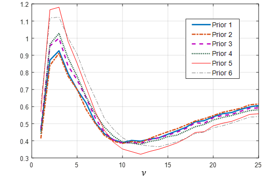
It is clear from Figure 1 that for between two and six the values for priors and are larger than those of the objective priors.
| Prior 1 | Prior 2 | Prior 3 | Prior 4 | Prior 5 | Prior 6 | |
| 1 | 94.10 | 94.50 | 94.20 | 93.90 | 91.15 | 92.75 |
| 2 | 94.25 | 94.80 | 93.80 | 93.95 | 86.55 | 92.00 |
| 3 | 97.55 | 97.15 | 97.20 | 96.45 | 88.65 | 96.70 |
| 4 | 97.75 | 97.70 | 98.60 | 97.70 | 97.70 | 98.80 |
| 5 | 97.10 | 97.20 | 97.30 | 98.05 | 99.30 | 98.40 |
| 6 | 97.30 | 97.15 | 97.60 | 98.00 | 99.40 | 98.25 |
| 7 | 97.90 | 97.55 | 98.20 | 97.95 | 99.75 | 98.55 |
| 8 | 97.30 | 97.60 | 97.80 | 97.75 | 99.75 | 98.30 |
| 9 | 98.35 | 97.65 | 98.20 | 97.75 | 99.30 | 98.60 |
| 10 | 97.70 | 97.05 | 97.80 | 98.25 | 98.85 | 98.20 |
| 11 | 96.90 | 96.60 | 97.20 | 98.30 | 98.90 | 97.75 |
| 12 | 97.60 | 97.15 | 97.90 | 98.45 | 99.75 | 97.95 |
| 13 | 97.55 | 97.45 | 97.80 | 97.85 | 99.65 | 98.55 |
| 14 | 97.80 | 97.45 | 98.10 | 98.10 | 99.35 | 98.65 |
| 15 | 97.85 | 96.80 | 97.60 | 98.15 | 99.10 | 98.45 |
| 16 | 97.85 | 97.10 | 98.50 | 98.60 | 99.10 | 98.35 |
| 17 | 97.75 | 97.95 | 98.20 | 97.85 | 99.30 | 98.65 |
| 18 | 97.10 | 96.30 | 97.00 | 97.80 | 98.90 | 98.30 |
| 19 | 97.65 | 97.30 | 98.00 | 97.70 | 99.00 | 98.25 |
| 20 | 96.80 | 97.00 | 96.60 | 97.80 | 98.50 | 97.40 |
| 21 | 95.90 | 96.30 | 96.50 | 97.70 | 98.10 | 97.50 |
| 22 | 97.00 | 96.10 | 97.50 | 97.60 | 98.80 | 98.15 |
| 23 | 97.15 | 97.10 | 98.00 | 97.05 | 98.70 | 97.85 |
| 24 | 96.55 | 95.55 | 96.70 | 98.45 | 97.40 | 97.75 |
| 25 | 97.20 | 97.10 | 98.40 | 97.35 | 99.00 | 98.60 |
| Mean | 97.118 | 96.864 | 97.388 | 97.540 | 97.758 | 97.708 |
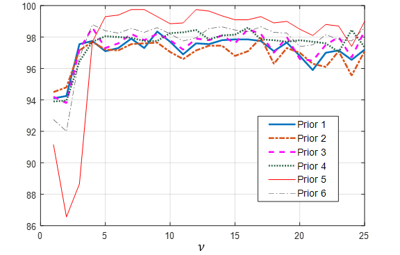
In Table 3 the frequentist coverage percentages of the 95% credibility intervals are given for a sample size of and 2000 simulations. In Figure 2 these intervals are illustrated graphically.
According to \citeasnoun[Figure 2, p. 329]fonseca08 the coverage percentages of the 95% credibility intervals for in the case of the Jeffrey’s-rule prior, are poor for . They also mentioned that for the Geweke prior, , the frequentist coverage is much smaller than the nominal level for small and is undesirably close to 1 for .
The results of \citeasnounfonseca08 differ somewhat from our results given in Table 3 and Figure 2. From Table 3 it can be seen that for the frequentist coverage percentage of the Geweke prior is smaller than the nominal level and for it is on average 98.98%. The coverage percentages of the Jeffreys-rule prior , however, do not differ much from those of the other objective priors (, and ). In the case of the coverage percentages, the reference (or probability-matching) prior seems to be the best because it has on average a 96.86% coverage.
| Prior 1 | Prior 2 | Prior 3 | Prior 4 | Prior 5 | Prior 6 | |
| 1 | 1.4863 | 1.4705 | 1.5211 | 1.6613 | 1.6616 | 1.7346 |
| 2 | 10.9029 | 10.2188 | 11.4415 | 11.4660 | 8.7877 | 13.1349 |
| 3 | 27.2776 | 25.6413 | 28.6591 | 27.4616 | 16.8940 | 31.0931 |
| 4 | 40.8181 | 39.1123 | 42.8603 | 46.0271 | 22.6912 | 49.8889 |
| 5 | 58.0892 | 54.0122 | 60.7860 | 57.8947 | 27.6600 | 70.0064 |
| 6 | 66.8981 | 64.0113 | 69.8454 | 70.4983 | 29.9378 | 80.6659 |
| 7 | 74.5588 | 72.6509 | 77.8293 | 78.6948 | 32.0676 | 91.6501 |
| 8 | 81.3848 | 78.6516 | 84.8817 | 88.3929 | 33.6076 | 98.8977 |
| 9 | 84.4323 | 80.7490 | 87.9760 | 94.3561 | 34.2755 | 105.0209 |
| 10 | 90.9408 | 87.5548 | 94.5730 | 96.4120 | 35.2627 | 109.2556 |
| 11 | 91.3351 | 87.6219 | 94.9579 | 104.1987 | 35.2547 | 110.6545 |
| 12 | 97.0578 | 93.8699 | 100.7701 | 103.0313 | 36.2704 | 114.0066 |
| 13 | 96.1922 | 93.0008 | 99.8689 | 105.4707 | 36.1493 | 117.2605 |
| 14 | 99.1662 | 95.2863 | 102.9146 | 110.7050 | 36.6309 | 122.5355 |
| 15 | 101.8962 | 97.7551 | 105.7096 | 108.7843 | 37.0405 | 124.0829 |
| 16 | 103.5499 | 100.0941 | 107.4031 | 115.3113 | 37.3834 | 126.0403 |
| 17 | 104.6025 | 100.4079 | 108.4889 | 114.0209 | 37.5741 | 126.7225 |
| 18 | 102.7811 | 99.5750 | 106.6120 | 115.6712 | 37.2385 | 126.3335 |
| 19 | 108.6713 | 104.4110 | 112.4989 | 115.4082 | 38.0129 | 129.7908 |
| 20 | 105.8102 | 102.0438 | 109.6180 | 115.2661 | 37.5957 | 129.2041 |
| 21 | 107.9256 | 104.7400 | 111.7811 | 115.8514 | 37.8954 | 131.9269 |
| 22 | 110.7806 | 106.7750 | 114.5896 | 116.6591 | 38.3138 | 132.9114 |
| 23 | 111.1055 | 107.3003 | 114.9879 | 117.8916 | 38.4163 | 133.3977 |
| 24 | 110.3250 | 105.5900 | 114.1435 | 120.3860 | 38.2195 | 133.3991 |
| 25 | 114.3742 | 110.4022 | 118.2419 | 122.1614 | 38.8475 | 137.3235 |
| Mean | 84.0945 | 80.9178 | 87.3184 | 90.9473 | 32.1475 | 101.8775 |
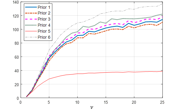
From Table 4 and Figure 3 it can be observed that has the shortest average interval lengths of all the objective priors. The prior that gives the shortest interval lengths is however , the Geweke prior, with interval lengths on average two and a half to three times shorter than those of the objective priors and with a coverage percentage of more than 95%. The worst performing prior seems to be .
Although the interval lengths of the objective priors for most of the 2000 simulations are quite small, a few extremely large lengths can have a big influence on the average interval length. A large interval length will occur if the observations in the sample are of such a nature that it is not clear if the data were drawn from a normal or -distribution. It is for this reason that the modes of the interval lengths are given in Table 5 and Figure 4.
| Prior 1 | Prior 2 | Prior 3 | Prior 4 | Prior 5 | Prior 6 | |
|---|---|---|---|---|---|---|
| 1 | 1.3918 | 0.9694 | 0.8824 | 1.0916 | 1.1767 | 1.1350 |
| 2 | 2.2132 | 2.1039 | 2.2849 | 2.2145 | 2.5818 | 2.2474 |
| 3 | 5.1277 | 5.1071 | 2.5923 | 5.3916 | 4.1166 | 5.4524 |
| 4 | 5.5141 | 5.8186 | 5.6744 | 6.1332 | 7.0209 | 6.2217 |
| 5 | 5.8345 | 6.4857 | 6.3385 | 6.8614 | 40.3448 | 6.9601 |
| 6 | 8.4593 | 6.7914 | 7.0016 | 7.1734 | 39.8707 | 7.2716 |
| 7 | 7.1246 | 6.5109 | 9.9536 | 6.8896 | 42.4445 | 9.7214 |
| 8 | 6.9421 | 7.2842 | 7.8857 | 10.4286 | 40.2139 | 10.5493 |
| 9 | 9.5604 | 7.1040 | 10.2161 | 7.5794 | 41.2099 | 162.6129 |
| 10 | 10.6371 | 9.9450 | 151.4783 | 156.0163 | 40.6707 | 178.7038 |
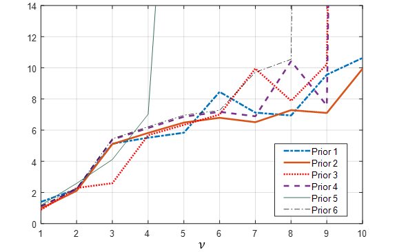
As before, the reference priors and seem to be the two best priors because the modes of their interval lengths are in general the smallest. The prior seems to be somewhat better than . The modes of the interval lengths of the priors and (the independence Jeffreys and the Jeffreys-rule priors) change dramatically for . From Table 5 it is clear that , the Geweke prior, is the worst prior for . It does well for and seems to do better than most of the priors for . The prior again seems to perform worst in this study.
4 Application
To compare the six priors on real data, a random sample of observations of the daily log-returns of IBM data is analysed. The original data set contains 2528 observations for the period from the of January 1989 to the of December 1998. The data are available from the ‘Ecdat’ R package [Rcoreteam, Croissant2015].
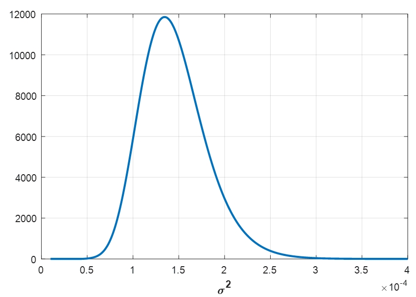
By using the prior and Gibbs sampling the posterior distribution of the parameters and are obtained and illustrated in Figures 5, 6 and 7. The resulting posterior statistics of for the six priors are summarized in Table 6. The conditional posterior distributions that were used in the Gibbs sampling procedure are given in Appendix C.
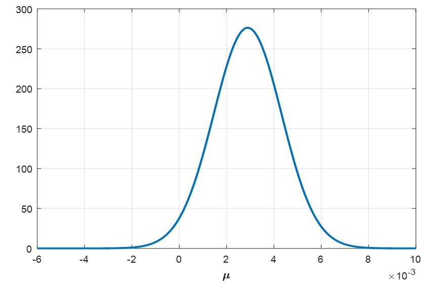
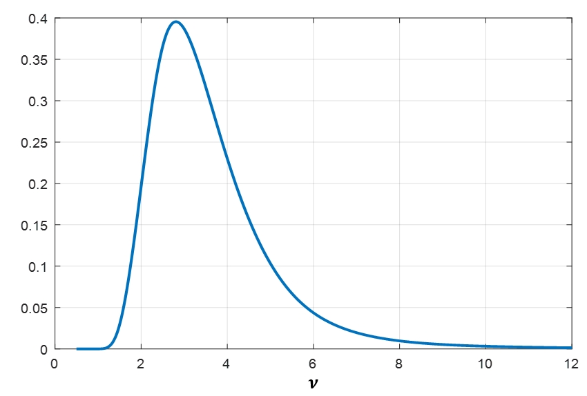
h! Prior Mean Median 95% Credibility Interval 1 3.6454 3.33 (1.851; 7.044) 2 3.6118 3.28 (1.797; 7.136) 3 3.7471 3.41 (1.830; 7.217) 4 3.7894 4.43 (1.860; 7.919) 5 4.3722 3.95 (2.064; 9.112) 6 3.9485 3.59 (1.940; 7.561)
It can be noticed that the posterior statistics of for the objective priors are for all practical purposes the same, but differ somewhat from those of the exponential () and the hierarchical () priors.
5 Discussion
The Student -distribution is of great importance for many economic and business data because is reduces the influence of outliers in model estimation and thus makes statistical analysis more robust.
Unfortunately, the estimation of , the number of degrees of freedom of the -distribution is not easy. The reason for this is the bad behaviour of the likelihood function for . To overcome the fact that the likelihood function does not vanish in the tail a prior distribution that tends to zero as tends to infinity should be applied. It is for this reason that two non-informative priors, and , have been derived for the parameters of the Student distribution. Both of these priors are reference priors while is also a probability-matching prior.
Our simulation studies illustrate the good frequentist properties of the posterior distributions associated to these priors. The focus has been on the relative square-rooted mean squared error from the posterior median and the 95% credibility intervals for a sample of size based on 2000 simulations. We have compared the frequentist properties of the two reference priors to four other priors (the Jeffrey’s-rule prior, the independence Jeffreys prior, the exponential prior and a hierarchical prior). Overall the two reference priors seem to give better results, especially if .
In Section 4 the six priors are compared on a real data set. A random sample of observations of the daily log-returns of IBM data is analysed. The results show that the posterior statistics of for the objective priors are for all practical purposes the same, but differ somewhat from those of the exponential and hierarchical priors.
References
- [1] \harvarditemBerger \harvardand Bernardo1992berger92 Berger, J. \harvardand Bernardo, J. \harvardyearleft1992\harvardyearright, ‘On the development of reference priors’, Bayesian Statistics 4, 35–60.
- [2] \harvarditemBlattberg \harvardand Gonedes1974blatt74 Blattberg, R. C. \harvardand Gonedes, N. J. \harvardyearleft1974\harvardyearright, ‘A comparison of the stable and student distributions as statistical models for stock prices’, The Journal of Business 47(2), 244–280.
-
[3]
\harvarditemBox \harvardand Tiao2011box11
Box, G. E. P. \harvardand Tiao, G. C. \harvardyearleft2011\harvardyearright, Bayesian Inference in Statistical Analysis, Wiley Classics Library,
Wiley.
\harvardurlhttps://books.google.co.za/books?id=T8Askeyk1k4C -
[4]
\harvarditemCroissant \harvardand Graves2020Croissant2015
Croissant, Y. \harvardand Graves, S. \harvardyearleft2020\harvardyearright,
Ecdat: Data Sets for Econometrics.
R package version 0.3-9.
\harvardurlhttps://CRAN.R-project.org/package=Ecdat - [5] \harvarditemDatta \harvardand Ghosh1995datta95 Datta, G. \harvardand Ghosh, J. \harvardyearleft1995\harvardyearright, ‘On priors providing frequentist validity for bayesian inference’, Biometrika 82(1), 37–45.
-
[6]
\harvarditemFernández \harvardand Steel1998fernandez98
Fernández, C. \harvardand Steel, M. F. J. \harvardyearleft1998\harvardyearright, ‘On bayesian modeling of fat tails and skewness’,
Journal of the American Statistical Association 93(441), 359–371.
\harvardurlhttps://www.tandfonline.com/doi/abs/10.1080/01621459.1998.10474117 - [7] \harvarditem[Fonseca et al.]Fonseca, Ferreira \harvardand Migon2008fonseca08 Fonseca, T. C. O., Ferreira, M. A. R. \harvardand Migon, H. S. \harvardyearleft2008\harvardyearright, ‘Objective bayesian analysis for the student-t regression model’, Biometrika 95(2), 325–333.
-
[8]
\harvarditemGeweke1993geweke93
Geweke, J. \harvardyearleft1993\harvardyearright, ‘Bayesian treatment of the
independent student-t linear model’, Journal of Applied Econometrics
8(S1), S19–S40.
\harvardurlhttps://onlinelibrary.wiley.com/doi/abs/10.1002/jae.3950080504 - [9] \harvarditemGnanadesikan \harvardand Kettenring2005gnan72 Gnanadesikan, R. \harvardand Kettenring, J. R. \harvardyearleft2005\harvardyearright, ‘Bayesian computation for logistic regression’, Computational Statistics and Data Analysis 48, 857–868.
-
[10]
\harvarditemJuárez \harvardand Steel2010juarez10
Juárez, M. A. \harvardand Steel, M. F. J. \harvardyearleft2010\harvardyearright, ‘Non-gaussian dynamic bayesian modelling for panel
data’, Journal of Applied Econometrics 25(7), 1128–1154.
\harvardurlhttps://onlinelibrary.wiley.com/doi/abs/10.1002/jae.1113 -
[11]
\harvarditemKotz \harvardand Nadarajah2004kotz04
Kotz, S. \harvardand Nadarajah, S. \harvardyearleft2004\harvardyearright,
Multivariate T-Distributions and Their Applications, Cambridge
University Press.
\harvardurlhttps://books.google.co.za/books?id=dmxtU-TxTi4C - [12] \harvarditemLiu1997liu97 Liu, C. \harvardyearleft1997\harvardyearright, ‘Ml estimation of the multivariate t distribution and the em algorithm’, Journal of Multivariate Analysis 63, 296–312.
- [13] \harvarditemPearn \harvardand Wu2005pearn05 Pearn, W. \harvardand Wu, C. \harvardyearleft2005\harvardyearright, ‘A bayesian approach for assessing process precision based on multiple samples’, European Journal of Operational Research 165(3), 685–695.
-
[14]
\harvarditemR Core Team2013Rcoreteam
R Core Team \harvardyearleft2013\harvardyearright, R: A Language and
Environment for Statistical Computing, R Foundation for Statistical
Computing, Vienna, Austria.
\harvardurlhttp://www.R-project.org/ -
[15]
\harvarditemRubio \harvardand Steel2015rubio15
Rubio, F. J. \harvardand Steel, M. F. J. \harvardyearleft2015\harvardyearright, ‘Bayesian modelling of skewness and kurtosis with
two-piece scale and shape distributions’, Electron. J. Statist. 9(2), 1884–1912.
\harvardurlhttps://doi.org/10.1214/15-EJS1060 -
[16]
\harvarditem[Vaneck et al.]Vaneck, Rodriguez-Ortiz, Schmidt \harvardand Manley1996vaneck96
Vaneck, T. W., Rodriguez-Ortiz, C. D., Schmidt, M. C. \harvardand Manley,
J. E. \harvardyearleft1996\harvardyearright, ‘Automated bathymetry using
an autonomous surface craft’, NAVIGATION 43(4), 407–419.
\harvardurlhttps://onlinelibrary.wiley.com/doi/abs/10.1002/j.2161-4296.1996.tb01929.x -
[17]
\harvarditemVilla \harvardand Rubio2018villa18
Villa, C. \harvardand Rubio, F. J. \harvardyearleft2018\harvardyearright,
‘Objective priors for the number of degrees of freedom of a multivariate t
distribution and the t-copula’, Computational Statistics & Data
Analysis 124, 197–219.
\harvardurlhttp://www.sciencedirect.com/science/article/pii/S0167947318300707 -
[18]
\harvarditemVilla \harvardand Walker2014villa14
Villa, C. \harvardand Walker, S. G. \harvardyearleft2014\harvardyearright,
‘Objective prior for the number of degrees of freedom of a t distribution’,
Bayesian Anal. 9(1), 197–220.
\harvardurlhttps://doi.org/10.1214/13-BA854 - [19] \harvarditemZellner1976zellner76 Zellner, A. \harvardyearleft1976\harvardyearright, ‘Bayesian and non-bayesian analysis of the regression model with multivariate student-t error terms’, Journal of the American Statistical Association 71(354), 400–405.
- [20]
Appendix A
This appendix provides derivations for the reference and probability-matching priors for the univariate Student -distribution. As in the case of the Jeffreys’ priors the derivations of these priors are based on the Fisher information matrix. Differentiation of the log likelihood functions twice with respect to the unknown parameters and taking expected values gives the Fisher information matrix.
where , and,
Proof of Theorem 2.2.
To derive the probability-matching prior , we need the inverse of the Fisher information matrix,
where
Let , where is the parameter of interest.
From this it follows that , and,
Therefore,
which means that,
This indicates that the probability-matching prior is:
because the differential equation . The probability-matching prior is therefore the same as the reference priors for the orderings , , and .∎
Appendix B
Proof of Theorem 2.4.
The proof will be given for . The proof for follows in a similar way. The posterior for is as follows:
where is the normalizing constant. We then have that:
Since if , it follows that, if , then
It is therefore only necessary to consider:
Since , it follows that,
Therefore,
| (1) |
The following formulae are valid:
| (2) |
where is Euler’s constant. It can also be shown that if we have that
and that, if ,
| (3) |
where is Riemann’s zeta function. Therefore Equations 2 3 gives
Since , it follows that, as ,
Therefore,
| (4) |
From Equation (2) it follows that,
Therefore,
and,
Remember that . By making use of Equation (4) and the fact that as , it follows that
Therefore, as ,
| (5) |
Substitute Equation (5) into Equation (1)and assume that . Then,
which follows from the fact that and , therefore , if . This means that if . A similar proof can be made for .∎
Appendix C
If , and , then . If the prior is used, then the following conditional posterior distributions can be derived:
| (6) |
where , , and ;
| (7) |
| (8) |
and,
| (9) |
By using Equations (6), (7), (8) and (9) and then Gibbs sampling, the unconditional posterior distributions of , and can be obtained.
In the case of , the degrees of freedom of the Chi-square distribution in Equation (7) changes to .