SETI strategy with FAST fractality

Abstract

We applied the Koch snowflake fractal antenna in planning calibration of the Five-hundred-meter Aperture Spherical radio Telescope (FAST), hypothesizing second-order fractal primary reflectors can optimize the orientated sensitivity of the telescope. Meanwhile, on the grounds of NASA Science Working Group Report in 1984, we reexamine the strategy of Search for Extraterrestrial Intelligence (SETI). A mathematical analysis of the radar equation will be performed in the first section, aiming to make it convenient to design a receiver system that can detect activities of an extraterrestrial civilization, according to the observable region of the narrowband. Taking advantage of the inherent potential of FAST, we simulate the theoretical detection of a Kardashev Type I civilization by a snowflake-selected reflecting area (Drake et al.).

1 Overview

At the outset, Dunning et al. put forward a blueprint for an L-band orientation cryogenic 19 multi-beam feed system (Dunning et al. 2017) in August 2017. The Stewart platform cabin (Li et al. 2017) represented an improvement over the CSIRO Parkes Observatory at the Australian National Telescope Facility (ATNF). In recent years, the scientific work at National Astronomical Observatories, Chinese Academy of Sciences (NAOC) has gradually expanded to possible recognition of extraterrestrial signals (Nan et al. 2011). In this section, we briefly review the status quo in application of a Search for Extraterrestrial Intelligence (SETI) theoretical framework to antenna design to provide a direct description of the fractal refinement of the Five-hundred-meter Aperture Spherical radio Telescope (FAST).

We start by introducing the holomorphic Helmholtz equation for a radiating antenna

$$\Delta u+k^{2}u=0\,.$$ (1)

Inspired by the target detection method mentioned in the Exotic Target Catalog (Lacki et al. 2020), we let function $s$ represent the probe  (Bayliss & Turkel 1980) for the stereoscopic survey (Appendix A)

$$u(d,\theta,\varphi)=\frac{{\rm e}^{-jR}}{R}\sum_{n}^{\infty}\frac{s_{n}(\theta,\varphi)}{R^{n}}\,,$$ (2)

where the denotations $\theta,\varphi$ are angular variables of the radiation. Based on extrapolating elliptical radiation characteristics of antenna detection in Appendix A, we introduce the polarized voltage V of the antenna receiver as ideal piezoelectricity

$${\textit{V}}(t)=\sum_{n}^{\infty}|C_{n}|{\rm e}^{j2\pi v_{n}t},\forall~{}C\in\mathfrak{R}^{+}\,.$$ (3)

In order to scale the polyphaser in Equation (3), we estimate the power spectrum in the Nyquist form. Suppose the density of the noise voltage across a resistor with complex impedance $Z$ is in thermal equilibrium (Nyquist 1928)

$${\rm d\overline{{\textit{V}}^{2}}}=4dk_{B}T_{\rm sys}v\cdot{\rm re}\{Z\}\left[0.5+\frac{1}{{\rm e}^{(hv/k_{B}T_{\rm sys})}-1}\right]{\rm d}v{.}$$ (4)

We claim the simplified excess noise ratio (ENR) from the time average for the band-pass filter

$$\overline{\dot{{\textit{V}}}}\approx 4dk_{B}T_{\rm sys}\Delta v=4d\times{\rm ENR}\,,$$ (5)

where the equivalent noise bandwidth (ENBW) has been established (Appendix B). To extend the expression of the noise factor $f$, we reference one of the applications for ideal intermediate frequency (IF) sampling receivers (e.g. the dual high-speed differential amplifier LTC6420-20 targeted at processing signals from DC to 300 MHz), described by the term

$$f=f_{1}+\sum_{k=2}^{m}f^{k}\left(\prod_{i=1}^{m-1}G_{i}\right)^{-1}\,,$$ (6)

where gain $G$ and the series is defined as $\{f^{k}\triangleq f_{k}-1|k=2,3,...,m\}$, and the relationship with the signal-to-noise ratio (SNR) is dimensionless

$$f=\rm SNR_{in}/SNR_{out}\,.$$ (7)

On the other hand, we define $P_{\rm on}$ and $P_{\rm off}$ to be the power level of the receivers measured at the moment of being switched on and off respectively, following the ratio

$$\eta_{\rm sw}=P_{\rm on}/P_{\rm off}$$ (8)

to do logarithmic processing of the noise figure (NF)

$${\rm NF}=10\log_{10}f=10\log_{10}\left(\frac{10^{\rm ENR/10}}{10^{\eta_{\rm s}/10}-1}\right)$$ (9)

concluding

$${\rm NF}={\rm ENR}-10\log_{10}(\eta_{\rm s}-1)\,.$$ (10)

For the photoelectric conversion of the feed cabin, we express the NF by considering temperature

$$\rm\frac{SNR_{in}}{SNR_{out}}=1+\frac{\emph{T}_{R}}{\emph{T}_{o}}$$ (11)

to substitute into the gain control that under the steady state intermediate frequency amplifier (IFA) (MK & Sushil 2000) yields

$$1+{\rm Y}=\frac{\rm ENR}{\eta_{\rm s}-1}\,{.}$$ (12)

Here, we set factor Y as the Johnson-Nyquist thermal noise representation of FAST from Equation (11)

$${\rm Y}=T_{\rm R}/T_{\rm o}\,,$$ (13)

yielding the noise temperature of the receiver

$$T_{\rm R}=T_{\rm o}\left(\frac{\rm ENR}{\rm\eta_{s}-1}-1\right)$$ (14)

at $T_{\rm o}=290{\,}{\rm K}$. Meanwhile, we consider the system loss; for all isotropic antennae, the system gain that occurs with the initial temporal distancing must be estimated

$$G_{\rm sys}=P_{\rm in}-P_{\rm re}+L_{\rm sys}\,.$$ (15)

After rearranging both sides of the equation, we have

$$P_{\rm in}-P_{\rm re} =|G_{\rm sys}-L_{\rm sys}|$$ (16)

$$=10\log_{10}\left[\eta\left(\frac{\pi d}{\lambda}\right)^{2}\right]\!-\!20\log_{10}\Delta v\!$$

$$\quad-\!20\log_{10}d\!-\!35.77,$$

where $P_{\rm re}$ denotes the interference signal level. We recall the noise power

$${\rm NF}=kT\Delta v_{\rm noise}\,,$$ (17)

which is standardized at 1 Hz, the back end of FAST is at room temperature (293 K) and the contribution to white noise is $-$174 dBm. In Peng (2008), for system gain with respect to receivers, the expression can be described as below

$$G_{\rm sys}= P_{\rm on}-{\rm NF}-10\log_{10}({\rm ENR}+1)$$ (18)

$$-10\log_{10}\Delta v+174\,,$$

where the antenna gain within a zenith angle of $\pi/6$ is 54.4$\sim$74.1 (dB) on average, and the sensitivity is ideally about 1600 $\rm(m^{2}{\,}K{{}^{-1}})$ if the efficiency of the telescope is 57%. On the other hand, Equation (17) can be decomposed as the level of noise on average

$$P=k_{B}T\Delta v$$ (19)

while we compute logarithm on both sides

$$\log_{10}P\cong\log_{10}(k_{B}T)+\log_{10}\Delta v\,,$$ (20)

which is directly proportional to the bandwidth $P\propto\Delta v$. For the purpose of measuring the sensitivity F, the system equivalent flux density (SEFD) must be introduced as a bridge

$${\rm SEFD}=\frac{2k_{B}T_{\rm sys}}{\eta A}\,,$$ (21)

where the physical collecting area of the telescope is $A$ and dimensionless efficiency factor $\eta\in[0,1]$ is normally between 0.5 $\sim$ 0.7 without distortion. From the perspective of a radio telescope, we define the effective collecting area

$$\eta\frac{G\lambda^{2}}{4\pi}=\eta A\equiv A_{\rm eff}\,.$$ (22)

In addition, according to experience studying military radars and TV station antennas, M. Zaldarriaga & A. Loeb claim that the point source sensitivity (PSS) of an interferometer composed of antennae may collect radiation that could be detected by SETI with redshifted 21 cm observation

$${\rm F_{PSS}}={\rm costant}\times\frac{\rm SEFD}{\sqrt{\Delta vt_{\rm ob}N_{\rm b}}}\,.$$ (23)

However, to estimate the constant, we assume that the receiver is optimized to ensure the SNR is reasonable. In the first step, the frequency domain criterion of the filter is defined by the complex conjugate spectrum. In other words, the contribution of the spectral function to SEFD can be expanded to

$${\rm SNR}(\tau) =\frac{\left[\int_{-\infty}^{+\infty}|\mathcal{S}(v)|^{2}{\rm d}v\right]^{2}}{2\pi\varrho\int_{-\infty}^{+\infty}|\mathcal{S}(v)|^{2}{\rm d}v}$$ (24)

$$=\frac{1}{2\pi\varrho}\int_{-\infty}^{+\infty}|\mathcal{S}(v)|^{2}{\rm d}v\overset{\text{def}}{=}{\rm SN{R}},$$

$$\quad\quad{\rm when}~{}~{}\tau=t,$$

where $\varrho$ represents the spectral power density from the background of stationary noise $\varrho$. Returning to Equation (23), we adjust the PSS equation

$$\framebox{${\rm F}={\rm SNR}\cdot\frac{\rm SEFD}{\sqrt{\Delta vt_{\rm ob}N_{\rm b}}}$}\,,$$ (25)

for the baseline $N_{\rm b}$ of sweeps that are observed for a time $t_{\rm ob}$ with a bandwidth $\Delta v$. We completed the proof for the sensitivity F. Considering the pulse repetition frequencies (PRF) with constant observation time, we find the relationship

$${\rm S_{Pmin}}\propto\frac{1}{\sqrt{N_{\rm b}}}\,,$$ (26)

where the minimal signal power is $\rm S_{Pmin}$. Given the physical antenna gain

$$G=\left(\frac{4\pi}{\lambda^{2}}\right)A_{\rm eff} =\left(\frac{4\pi}{\lambda^{2}}\right)\eta A=\eta\cdot\frac{4\pi}{\lambda^{2}}\cdot\frac{G_{\rm rec}\lambda^{2}}{4\pi}$$ (27)

$$=\eta\cdot\frac{4\pi}{\lambda^{2}}\cdot\frac{\pi d^{2}}{4}=\eta\left(\frac{\pi d}{\lambda}\right)^{2}$$

where the gain of the transmitter has been defined by power density $\varrho$

$$G=\frac{\varrho(\theta,\phi)}{P_{\rm tr}/4\pi d^{2}}\,,$$ (28)

we claim the power for the receiver

$$P_{\rm rec}={\rm S_{p,rec}}A_{\rm eff}=\frac{G_{\rm tr}P_{\rm tr}}{4\pi d^{2}}\cdot\eta\left(\frac{G_{\rm rec}\lambda^{2}}{4\pi}\right)$$ (29)

so that we restate the Friis transmission for the gradient of its power radiation as

$$P_{\rm rec} =\cos^{2}(vt)\cdot\eta\cdot\frac{G_{\rm rec}G_{\rm tr}P_{\rm tr}c^{2}}{(4\pi dv)^{2}}$$ (30)

$$\equiv{\rm NPF}\cdot\frac{\eta G_{\rm rec}G_{\rm tr}P_{\rm tr}c^{2}}{(4\pi dv)^{2}},$$

and the effective radiated power (ERP) that is related to the signal power within the antenna

$${\rm S_{P}}=\frac{GP}{4\pi d^{2}}\cdot\frac{\sigma}{4\pi d^{2}}\cdot\frac{G\lambda^{2}}{4\pi}{.}$$ (31)

Calculating the ERP

$${\rm S_{P}}={\rm ERP}\cdot\frac{\sigma A_{\rm eff}}{16\pi^{2}d^{4}}\,.$$ (32)

Returning to Equation (31), we express the signal power

$${\rm S_{P}} =\left(\frac{1}{4\pi d^{2}}\cdot\frac{4\pi\eta A}{\lambda^{2}}\cdot P\right)\left(\frac{\sigma}{4\pi d^{2}}\right)\left(\frac{1}{4\pi}\cdot\frac{4\pi\eta A}{\lambda^{2}}\cdot\lambda^{2}\right)$$ (33)

$$=\frac{P\sigma\eta^{2}A^{2}}{4\pi d^{4}\lambda^{2}}\,.$$

In view of the minimal signal having a local detection for recording the signature, we obtain the biquadratic distance

$$d_{\rm max}^{4} \approx\frac{P\sigma GA_{\rm eff}^{2}}{4\pi\lambda^{2}{\rm S_{P,min}}}=\frac{P\sigma GA_{\rm eff}^{2}}{4\pi\lambda^{2}[P_{\rm int}\cdot f\cdot({\mathop{}_{t\in\mathbb{R}}^{\rm int}\rm SNR_{out}})]}$$ (34)

$$\leavevmode\resizebox{422.77661pt}{}{$=P\sigma A_{\rm eff}^{2}/\left[4\pi\lambda^{2}k_{B}T_{0}\Delta v\cdot\left(\frac{N_{\rm out}}{Gk_{B}T_{0}\Delta v}\right)\left(\frac{S_{\rm out}}{N_{\rm out}}\right)_{{\rm min},T}\right]{.}$}$$

When the radar temperature is fixed, the radius has been determined

$$d_{\rm max}=\sqrt[4]{\frac{P\sigma A_{\rm eff}^{2}}{4\pi S_{\rm P,min}\lambda^{2}}}\,{.}$$ (35)

The issue of multiple SNR values from panel points with R/T components is not the case in this section. In addition, we notice that the fading depth in the antennae needs to be recalled (Nakagami 1960)

$$m=\rm\frac{E^{2}[RSL]}{Var[(RSL)^{2}]}\,,$$ (36)

which is related to received signal level (RSL) while the average signal power for the antenna in the formula is $\rm E[RSL^{2}]$. Drake et al. (1984) mentioned that no-slot joint exists to define the range limitation $d_{\rm max}$ with one degree of freedom

$$d_{\rm max} =\sqrt{\frac{AP}{4\pi mk_{B}T_{0}\Delta v}}$$ (37)

$$=\sqrt{\left(\frac{\eta\pi l^{2}}{4}\right)\left(\frac{P}{4\pi mk_{B}T_{0}\Delta v}\right)}$$

$$=\sqrt{\frac{l^{2}\eta P}{16mk_{B}T_{0}\Delta v}}\,{.}$$

The notation in Eq. (37) represents diameter $l\in\mathbb{N}^{+}$ and aperture efficiency $\eta$, respectively

$$d_{\rm max}=\frac{l}{4}\sqrt{\frac{\eta P}{\pi mk_{B}T_{0}\Delta v}}\,.$$ (38)

Taking out the scattering formula for the receiving power, we adopt the spheral radiation description

$${\rm EIRP}=\frac{P_{\rm rec}}{G_{\rm rec}}\cdot\left(\frac{v}{c}\right)^{2}\cdot(4\pi d)^{2}.$$ (39)

The ratio

$${\rm SNR}=\frac{A_{\rm eff}\cdot{\rm EIRP}}{4\pi d^{2}k_{\rm B}T_{\rm sys}\Delta v}$$ (40)

also satisfies the equation

$${\rm EIRP}=G_{\rm in}+10\log\Delta v\,.$$ (41)

Secondarily, we introduce the power of transmitting antenna $P_{\rm tr}$ so that the distance of the transmitter can be rewritten as

$$d_{\rm max}=\sqrt{\frac{G_{\rm tr}P_{\rm tr}}{4\pi{\rm S_{min}}}}=\sqrt{\frac{\rm EIRP}{4\pi{\rm S_{min}}}}\,.$$ (42)

Vice versa, Equation (42) is associated with the cut sphere representation

$${\rm EIRP}={\rm S}_{\rm min}(4\pi d_{\rm max}^{2}),$$ (43)

which is equivalent to the sensitivity

$$\framebox{${\rm EIRP}={\rm F}\cdot 4\pi d_{\rm max}^{2}$}\,.$$ (44)

Considering the actual performance of non-solid transmitters, the EIRP calculation of FAST must be bypassed. For the scheme design of the SETI task, we emphasize the transmission efficiency with the high-level block diagram of the ROACH board development (e.g Xilinx Virtex 6 of a field-programmable gate array (FPGA) or ADC1X26G layout) from the FAST backend (Zhang et al. 2020), which can also detect prebiotic molecules.

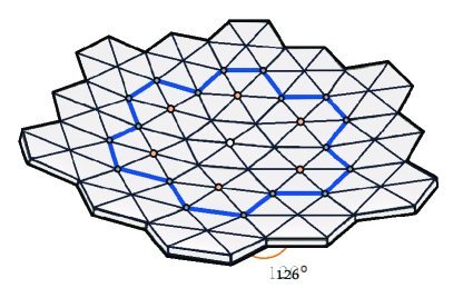
Figure 1: A part of the local fractalized main reflector. This displays iteration $n=2$. The center of the aperture is the 19 multibeam feed located at the coordinate (498956.8651, 2838440.713, 838.32178).

2 Fractalization of the aperture

Considering that FAST incorporates the Gregorian antenna design and its reflector is composed of perforated panels of size $1.5{\,}\rm m\times 1.5{\,}\rm m$ around the feed cabin, we invert the potential of the antennae to be able to trace the object. For example, it can detect a fast radio burst (FRB) event with two peaks (FRB 200428) (Lin et al. 2020) and a pulsar in local group M31 with $3.6\times 10^{5}$ s of observing time by dynamically deforming its elliptical shape (Jiang et al. 2019). Interestingly, we realized that one of the unique aspects of FAST, the cross-sectional area of the whole paraboloid $A_{\rm F}$, motivated us to reconceive the shape of FAST from geometrical iteration: we assume $2^{\rm nd}$ order Koch fractals relying on the iterated function system (IFS) technique. Considering that the observed structure of the antenna, located in the local universe, satisfies the mechanical similarity of a Julia set (Chen & Zhang 2019), we build an affine transformation set within a complex space which is similar to the process of altering the sectional area A, i.e., the Hutchinson operator used in fractal scaling

$$\mathcal{H}(A)=\bigcup_{k=1}^{m}w_{k}(A)\,.$$ (45)

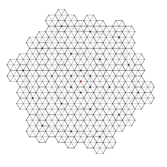
Figure 2: The blue-marked edges in Fig. 2 represent the partial deformation from star tracking. The whole area of FAST is composed of 10 728 identical triangular shaped reflectors. Each actuator node can be represented in Cartesian coordinates. Considering the mechanical support, we claim the local spatial coordinates for every cable element of FAST $\mathscr{Q}_{\rm FAST}=\rm[\textbf{X,Y,Z}]^{T}$, where these matrices X, Y and Z are sets of actuator node positions.

We introduce the Hohlfield-Cohen-Ramsey principle (HCR) (Hohlfeld & Cohen 1999), which describes the sufficient conditions for all frequency-independent antennas. The nature of the transformation produces

$$(\alpha A)\bigcap A=\alpha A,\alpha\in\mathbb{R}\,.$$ (46)

During the dimensional continuity stated in Equation (45), we define the coordinate spacing

$$\mathfrak{Z}=|{\rm z}_{i}-{\rm z}_{j}|,\quad i\neq j\,,$$ (47)

in which each $z$ denotes the coordinate of the actuator, and the total length of the broken line described by the proportion increases

$$\mathcal{L}=\left(\frac{4}{3}\right)^{n}\mathfrak{Z}\,.$$ (48)

Referring to research in 2003, K. J. Vinoy et al. first evaluated the relationship between the size of an antenna and generalized Koch fractal $D$ with respect to the angular dependence (Vinoy et al. 2003)

$$D=\frac{\log n}{\log(1/\xi)}\,{.}$$ (49)

The notation $\xi\in\rm\mathbb{R}$ is the scale factor of the snowflake, which is dependent upon the angle

$$\frac{1}{\xi}=\frac{1}{2(1+\cos\theta)}\,.$$ (50)

In this case, we substitute $n=4$, and let each edge angle of FAST consist of a unit triangular board with $\theta=60^{\circ}$, which can be described by Equation (49). Thus, each affected actuator obeys the relation

$$D =\frac{\log 4}{\log\{2(1+\cos(\pi/3))\}}$$ (51)

$$=\frac{\log 4}{\log 3}\approx 1.26185951\,.$$

For a pentagonal deformation, according to the practical investigation of FAST, these angles are $\theta_{1}=54^{\circ}$ and $\theta_{2}=72^{\circ}$. Especially for the junction between the local main reflectors, their dimensions through the Koch curve calculation are expressed as

$$(D_{1},D_{2})\approx(1.19974868,0.229966453).$$ (52)

From the point of view of the least disturbance on the performance of the fractal antenna

$$\epsilon(D,D_{1})<\epsilon(D,D_{2})\,,$$ (53)

the surface deformation at the angle of 54 degrees may have the minimum error $\epsilon$. On the other hand, one of the potentials that can be explored in FAST is the geometrical curve-fitting approach, and it is utilized to obtain an approximate formula for the design, which belongs to the area of recursive IFS. From the perspective of power electronics, we demonstrate one of the original ideas of the mechanism, for the input impedance through the fractalization

$$Z_{f}=Z_{\rm in}\left[1-(1+0.9\log 4)\frac{\log D}{D}\right]^{2}{.}$$ (54)

Substituting $D_{1}$ into Equation (54), we obtain the impedance to express the fractalized resistance

$$Z_{f}\approx 0.807\cdot Z_{\rm in}\,.$$ (55)

As the resistivity of the main-metallic aluminium is about 2.65 ohm km^-1 per square millimeter cross-sectional area, we estimate a rough value of the fractalized resistance is 2.13855 ohm km^-1 per square millimeter. Upon comparison, the value decreases by 19.3%. This case shows that the iteration in calculating the $2^{\rm nd}$ order Koch snowflake may develop to detect a low-frequency event in SETI backend improvement. We suppose that the fatigue stress tensor of the local cable network is within a reasonable range of the Miner criterion, and the adjusted shape of the reflecting surface does not violate the limitation of proportional-integral-derivative (PID) control performance of hydraulic actuators. It is only necessary to change the axial position of several groups of actuator nodes of the cable net slightly, so that the tracking area of the pulsar will generate a shape of up to $2^{\rm nd}$ order for the aluminium panels composing the Koch fractal antenna. The corollary is that the illustration depicted in Figure 2 can be referenced to develop a strategy utilizing sensitivity of fractal-area calibration (FAC).

3 Discussion

Since the main reflector of FAST is a deformable receiver composed of 2000 actuator units, using the finite Koch snowflake antenna iteration, we investigate the feasibility of applying it to a radio telescope such as FAST, aiming at optimizing the sensitivity and the observation capability for very long baseline interferometry (VLBI). From the ellipticity of EIRP to the influence of sensitivity equation for technosignatures, we incorporate various aspects, including the assumption of a second-order fractal antenna for the estimation of different intersection angles to find a suitable deformation of reflectors. We hope to apply a fractal antenna in the future and try to implement such correction to FAST, to optimize observations for SETI. Even if such a signal is like looking for a needle in a haystack, we believe it will improve additional opportunities for possible exobiological communication.

Appendix A

Define a Lie group acting on an electromagnetic field

$$L[\boldsymbol{\mathfrak{E,H}}]=L[\boldsymbol{\mathfrak{E}}]\otimes L[\boldsymbol{\mathfrak{H}}]\,.$$ (56)

According to the work by A. Bayliss & E. Turkel (Bayliss et al. 1982), Equation (2) has been extended to spherical coordinates. In such a case, the radiation $u$ is analytic, uniform and convergent if $n>1$. The series mentioned in reference Bayliss & Turkel (1980) is convergent, and can be obtained in a spherical form

$$R^{m}u(d,\theta,\varphi)= \sum_{n=1}^{m}R^{l-n}s_{n}(d,\theta,\varphi)$$ (57)

$$+\sum_{n=m+1}^{\infty}R^{l-n}s_{n}(d,\theta,\varphi)\,,$$

where $R=\alpha d$ and $\alpha\in\mathbb{N}$, multiplying by the order of $1/R$ to the radius. In the case of spherical harmonics, we express the signal function as (Bayliss et al. 1982)

$$s_{n}(\theta,\varphi)= \left[\frac{1}{n!(2j)^{n}}\right]\cdot\prod_{i=0}^{n}\left\{i(i-1)+\left[\frac{1}{\sin\theta}\frac{\partial}{\partial\theta}\right.\right.$$ (58)

$$\left.\left.+\left(\sin\theta\frac{\partial}{\partial\theta}\right)+\frac{1}{\sin^{2}\theta}\frac{\partial^{2}}{\partial\varphi^{2}}\right]\right\}s_{0}(\theta,\varphi).$$

Once the radial motion is asserted, the ERP on a 2D reference frame is the extension of electromagnetic circular polarization.

Appendix B

For the first stage receiver of a THz radar, we have the assumption: in a large-scale displacement survey, we intuitively regard the uncertainty principle in a homogeneous universe fits the narrowband approximation

$$\log\left(\frac{c+\textbf{v}}{c-\textbf{v}}\right)=\sum_{n=0}^{\infty}\frac{2}{2n+1}\cdot\left(\frac{\textbf{v}}{c}\right)^{2n+1}\thickapprox\frac{2\textbf{v}}{c}\,,$$ (59)

where the Doppler frequency

$$v_{\rm D}=-\frac{2\textbf{v}}{\lambda}\,{.}$$ (60)

The spectral energy can be written as

$$\frac{2v}{c}<< \left\{\left[\frac{\int(v_{0}-v_{\rm cut})^{2}|s_{1}(v)|^{2}{\rm d}v}{\int|s_{1}(v)|^{2}{\rm d}v}\right]\right.$$ (61)

$$\left.\times\left[\frac{\int(t_{0}-t_{\rm cut})^{2}|s_{1}(t)|^{2}{\rm d}t}{\int|s_{1}(t)|^{2}{\rm d}t}\right]\right\}^{-1}.$$

We represent in short

$$\left|\frac{v_{\rm D}}{v_{\rm cut}}\right|<<\delta v$$ (62)

while the sampling loss of the narrowband

$$\delta v\cong\frac{1}{\Delta v\Delta t}$$ (63)

is neglected. On the other hand, the normalized ambiguity function of a Doppler constant for narrowband will be

$$\frac{\iint_{-\infty}^{+\infty}\left|\int s_{2}(t)s_{1}^{*}(t-\tau){\rm e}^{2\pi jvt}{\rm d}t\right|^{2}{\rm d}\tau{\rm d}v}{\left|\int s_{1}(t)s_{1}^{*}(t){\rm d}t\right|^{2}}=1.$$ (64)

If the echnosignature is multi-point noise, we may intuitively see it as the geometrical center of the spectrum

$$\Delta v=\frac{\sum_{i}B_{i}\Delta v_{i}{\rm a}_{i}}{\sum_{i}B_{i}{\rm a}_{i}}\,,$$ (65)

where the delay frequency is $\Delta v_{i}$, corresponding to each R/T site from the target connection to the area, $B_{i}$ is the component weight and ${\rm a}_{i}$ is the delay amplitude for each site. In a non-relativistic regime

$$\Delta t=\frac{\sum_{i}B_{i}\Delta t_{i}{\rm a}_{i}}{\sum_{i}B_{i}{\rm a}_{i}}\,.$$ (66)

Overall, we define the response H and conveniently give the orthogonal expression of the ENBW for ideal IFA in the receiver

$$B=\frac{1}{|{\rm H}(v_{\rm max})|^{2}}\int_{0}^{\infty}|{\rm H}(v)|^{2}{\rm d}v\,.$$ (67)

Appendix C

See Table 1.

Table 1: GLOSSARY

Symbol	Meaning
$\omega$	Angular frequency (rad sec-1)
$k_{\rm B}$	Boltzmann’s constant ($1.38\times 10^{-23}$ J K-1)
$A$	Collecting area of the antenna ($\rm m^{2}$)
$v$	Frequency (Hz)
S	Flux density
$G$	Gain
$\theta,\varphi$	Intersection angle
$\delta v$	Narrow bandwidth
$N_{\rm b}$	Number of baselines
$t$	Observing time (s)
$\eta$	Observation efficiency
$\Delta v$	Observing channel bandwidth
$d$	Radius path or distance (m)
$T_{\rm sys}$	System noise temperature (K)
$c$	Speed of light ($2.99\times 10^{8}$ m s-1)
F	Sensitivity ($\rm m^{2}{\,}K{{}^{-1}}$)
$S_{\rm P}$	Signal power
v	Velocity (m s-1)
$\lambda$	Wavelength
ENBW	Equivalent noise bandwidth
ENR	Excess noise ratio
EIRP	Effective isotropic radiated power
HCR	Hohlfeld-Cohen-Rumsey principle
IF	Intermediate frequency
IFS	Iterated function system
NF	Noise figure
NPF	Nonlinear phase factor
PRF	Pulse repetition frequencies
RSL	Received signal level
SEFD	System equivalent flux density
SNR	Signal noise ratio

References

- Abraham & Matias (2006) Abraham, L., & Matias, Z. 2006, J. Cosmology Astropart. Phys, 2007, 020
- Bayliss & Turkel (1980) Bayliss, A., & Turkel, E. 1980, Communications on Pure and Applied Mathematics, 23, 707
- Bayliss et al. (1982) Bayliss, A., Gunzburger, M., & Turkel, G. E. 1982, Siam Journal on Applied Mathematics, 42, 430
- Chen et al. (2020) Chen, R.-R., Zhang, H.-Y., Jin, C.-J., et al. 2020, \raa, 20, 020
- Chen & Zhang (2019) Chen, S., & Zhang, T.-J. 2019, Results in Physics, 15, 102548
- Claudio (2012) Claudio, M. 2012, International Journal of Modern Physics D
- Drake et al. (1984) Drake, F., Wolfe, J. H., & Seeger, C. L. 1984, NASA Technical Paper, 2244
- Dunning et al. (2017) Dunning, A.,Bowen, M.,Castillo, S., et al. 2017, URSI GASS
- Hohlfeld & Cohen (1999) Hohlfeld, R. G., & Cohen, N. 1999, Fractals-complex Geometry Patterns and Scaling in Nature and Society, 7, 79
- Jiang et al. (2019) Jiang, P., Yue, Y.-L., Gan, H.-Q., & et al. 2019, Science China: Physics, Mechanics and Astronomy, 062, 959502
- Kardashev (1985) Kardashev, N. S. 1985, in The Search for Extracterrestrial Life: Recent Developments, Proc. IAU Symp. (Dordrecht: D. Reidel Publishing Co.), 112, 497
- Lacki et al. (2020) Lacki, Brian C., Brzycki, B., et al. 2020, arXiv e-prints, (arXiv:2006.11304)
- Li et al. (2017) Li, Q.-W., Jiang, P., & Nan, R.-D. 2017, Journal of Mechanical Engineering, 53, 62
- Lin et al. (2020) Lin, L., Zhang, C. F.and Wang, P., et al. 2020, Nature, 587, 63
- MK & Sushil (2000) MK, R., & Sushil, R. 2000, Indian journal of Radio and Space physics, 29, 363
- Nan et al. (2011) Nan,R.-D., Li,D.,Jin,C.-J., et al.2011, International Journal of Modern Physics D Gravitation Astrophysics & Cosmology, 989
- Nakagami (1960) Nakagami, M. 1960, in Statistical Methods in Radio Wave Propagation, ed. W. C. Hoffman (Pergamon), 3
- Nyquist (1928) Nyquist, H. 1928, Physical Review, 32, 110
- Peng (2008) Peng, B., Li, J.-B., & Piao, T.-Y. 2008, PUBLICATIONS OF THE ASTRONOMICAL SOCIETY OF THE PACIFIC, 120, 625
- Vinoy et al. (2003) Vinoy, K., Abraham, J. K., & Varadan, V. K. 2003, IEEE Transactions on Antennas and Propagation, 51, 2296
- Zhang et al. (2020) Zhang, Z.-S., Werthimer, D., Zhang, T.-J., Jeff, C., et al. 2020, The Astrophysical Journal,891,174