Spin-orbit coupling in organic microcavities: Lower polariton splitting, triplet polaritons, and disorder-induced dark-states relaxation

Abstract

Using an extended Tavis-Cummings model, we study the effect of the spin-orbit coupling between the singlet and the triplet molecular excitons in organic microcavities in the strong coupling regime. The model is solved in the single excitation space for polaritons, which contains the bright (permutation symmetric) singlet and triplet excitons, as well as the dark bands consisting of the nonsymmetric excitons of either type. We find that the spin-orbit coupling splits the lower polariton into two branches, and also creates a triplet polariton when the cavity mode is in resonance with the triplet excitons. The optical absorption spectrum of the system that can reveal this splitting in experiments is presented and the effect of disorder in exciton energies and couplings is explored. An important consequence of the disorder in the spin-orbit coupling — a weak coupling between the otherwise decoupled bright and dark sectors — is explored and detailed calculations of the squared transition matrix elements between the dark bands and polaritons are presented along with derivation of some approximate yet quite accurate analytical expressions. This relaxation channel for the dark states contains an interference between two transition paths that, for a given polariton state, suppresses the relaxation of one dark band and enhances it for the other.

I Introduction

The role of strong matter-light coupling Lidzey et al. (1998) in modifying and determining various physical properties has been extensively studied over the past two decades. Some important examples include the formation of polariton condensates Kasprzak et al. (2006); Keeling and Kéna-Cohen (2020) effect on superconducting phases Mitrano et al. (2016); Schlawin et al. (2017), charge and energy transport Feist and Garcia-Vidal (2015); Hagenmüller et al. (2017); Schäfer et al. (2019); Zeb et al. (2020), and chemical reaction rates Thomas et al. (2019); Herrera and Spano (2016); Galego et al. (2016, 2017); Martínez-Martínez et al. (2018); Ebbesen (2016); Feist et al. (2017); Ribeiro et al. (2018). Organic microcavities form an important class of systems that exhibit the strong matter-light coupling where the presence of the intramolecular vibrations and the triplet molecular excitons significantly enriches the prospects. The vibronic coupling and polaronic effects in these systems are very important and usually included in the models Nazir and McCutcheon (2016); Zeb et al. (2020). However, the spin-orbit coupling between the singlet molecular exciton and the triplet molecular excitons in organic microcavities has gained attention only very recently Polak et al. (2020).

The focus has been primarily on the energy landscape. The triplet excitons in organic molecules lie below the singlet excitons (by the exchange splitting ${J\sim 0.5-1~{}eV}$) and the singlet excitations relax to them (intersystem crossing, ISC Dias et al. (2013)). However, thermally activated processes (reverse intersystem crossing, RISC Dias et al. (2013)) can transfer the excitations from the triplet states to the singlet states. Compared to the singlet excitons that couple to the light and make polaritons, the electronic pumping of organic microcavities creates three times as many triplets and it is desired to make them emissive or use them to increase the polariton population for condensation or lasing. Thermally activated delayed fluorescence (TADF) Kaji et al. (2015); Wong and Zysman-Colman (2017); Yin et al. (2020), an exciting phenomenon that has attracted huge interest recently, exploits the RISC. RISC depends crucially on two quantities, (i) the size of the energy barrier and (ii) the transition matrix elements between the two types of excitations. The strength of the matter-light coupling in organic microcavities that is experimentally achievable has increased over time and recently it was demonstrated to even bring the lower polariton (LP) below the triplet exciton state, the so called inverted regime Eizner et al. (2019), allowing even a barrier-free RISC Yu et al. (2021). The matrix elements can originate from the spin-orbit coupling and thus can be increased by using heavy metals that have a larger atomic spin-orbit coupling and hence render a greater singlet character to the triplet state and vice versa Baldo et al. (1998); Adachi et al. (2001); Kawamura et al. (2005); Yersin et al. (2011). However, it does not matter how large the spin-orbit coupling is, the matrix elements still constitute a serious issue here. This is explained in the following.

For $N$ emitters coupled to a common cavity mode, there is a single bright state that creates two polaritons and ${N-1}$ “dark” states that do not couple to the cavity at all Ribeiro et al. (2018). In organic microcavities, this implies an overwhelmingly large density of states of such uncoupled singlet states that form an excitation reservoir Ribeiro et al. (2018); Eizner et al. (2019); Polak et al. (2020). Even when the spin-orbit coupling is large, the polaritonic subsystem cannot fully benefit from the triplet excitations because, as we show later, they would predominantly populate the dark singlet reservoir. The only sizable matrix elements connecting the triplet sector to the polaritons exist for a single permutation symmetric triplet excitation. There are ${N-1}$ nonsymmetric triplets that all couple to the singlet reservoir only. The fact that the high density of such dark singlet and triplet excitations dominates the dynamics and keeps the molecular excitations from the light emission has also been found recently Eizner et al. (2019); Martínez-Martínez et al. (2019). These dark states relax to the emissive polaritonic state very slowly Agranovich et al. (2002, 2003). The intramolecular vibrations of organic molecules can act as a heat bath and usually play an important role in the relaxation dynamics of excitations in organic microcavities Litinskaya et al. (2004); Michetti et al. (2009). In recent years, various theoretical del Pino et al. (2018); Groenhof et al. (2019); Sommer et al. (2021) and experimental Eizner et al. (2019); Polak et al. (2020); Yu et al. (2021); Mewes et al. (2020); Wers’́all et al. (2019); Xiang et al. (2019) works explored the relaxation pathways and dynamics of polaritons and dark states in these systems. It is interesting to explore new ways to relax the dark states to polaritons as it could help increase the polariton density for various applications.

In this work, we explore the effect of the spin-orbit coupling on the nature and dynamics of polaritons and the dark states in an organic microcavity using an extended Tavis-Cummings (TC) model Tavis and Cummings (1968). As shown in Fig. 1, the $\ket{LP}$ originating from the coupling $\omega_{R}$ between the (bright or symmetric) singlet exciton $\ket{{\mathcal{S}_{0}}}$ and the cavity mode can be made resonant to the triplet excitons as $\omega_{R}$ approaches $J$. In such a case, the effect of the spin-orbit coupling between the $\ket{{\mathcal{S}_{0}}}$ component in $\ket{LP}$ and the symmetric triplet $\ket{{\mathcal{T}_{0}}}$ becomes significant, requiring to treat the two couplings (the light-matter coupling and the spin-orbit coupling) on an equal footing; i.e., the spin-orbit coupling should not be treated as a “weak” coupling. It splits $\ket{LP}$ into $\ket{LP_{\pm}}$, both of which contain $\ket{{\mathcal{T}_{0}}}$ along with $\ket{{\mathcal{S}_{0}}}$ but have no interaction with the dark states $\ket{{\mathcal{S}_{j}}}$ and $\ket{{\mathcal{T}_{j}}}$ in a clean system. It is known that an energetic disorder can couple $\ket{{\mathcal{S}_{j}}}$ to $\ket{{\mathcal{S}_{0}}}$ (leading to finite optical absorption by $\ket{{\mathcal{S}_{j}}}$ Houdré et al. (1996); Ćwik et al. (2016)). This is also true for $\ket{{\mathcal{T}_{j}}}$ and $\ket{{\mathcal{T}_{0}}}$. We will show in this article that a disorder in the spin-orbit coupling can weakly couple the bright and dark sectors of different character; i.e., it couples $\ket{{\mathcal{S}_{j}}}$ to $\ket{{\mathcal{T}_{0}}}$, and $\ket{{\mathcal{T}_{j}}}$ to $\ket{{\mathcal{S}_{0}}}$, which induces transitions between them and hence can cause relaxation of the dark bands $\ket{\mathcal{D}_{j,\pm}}$ (that contain $\ket{{\mathcal{S}_{j}}}$ and $\ket{{\mathcal{T}_{j}}}$) to, for instance, the lowest energy polaritons, $\ket{LP_{-}}$. This could potentially be useful to increase the polariton population for an enhanced incoherent light emission or, more importantly, for creating a polariton condensate or laser.

In the following, we first consider a clean system in secs. II and III to explore the effects of the spin-orbit coupling in organic microcavities. We find that, similar to the TC model, we can decouple the system into bright and dark sectors, which make polaritons and dark bands in this case. We find that the spin-orbit coupling splits the lower polariton $\ket{LP}$ into two branches $\ket{LP_{\pm}}$ and at a certain location in the dispersion, we can have triplet polaritonic states. The optical absorption spectrum of the system, which can show $\ket{LP_{\pm}}$ in the experiments, is also presented. In sec. IV, we consider the robustness of the results of the clean model against disorder both in energies and couplings (at typical disorder strengths) by looking at its effects on the optical absorption spectrum. Finally, in sec. V, we show that the disorder in the spin-orbit coupling weakly couples the bright and the dark sectors, which induces transitions between polaritons and the dark bands and thus opens a channel for the dark states to relax into the lowest energy polaritons. We perform detailed calculations of the corresponding transition matrix element and present numerical results as well as accurate analytical expressions.

Figure 1: A sketch of the energy level diagram showing the cavity state $\ket{1_{P}}$ along with the singlet and triplet bright ($\ket{\mathcal{S}_{0}},\ket{\mathcal{T}_{0}}$) and dark ($\ket{\mathcal{S}_{j}},\ket{\mathcal{T}_{j}}$) molecular states. The coupling between the singlet exciton and the cavity photon state creates the lower and the upper polaritons, $\ket{LP}$ and UP. Roughly speaking, the $\ket{LP}$ couples to the triplet molecular exciton state and produces LP_±. The bright and the dark spaces that are decoupled for a clean system, as shown here, get weakly coupled when a disorder in the spin-orbit coupling is present.

II Model and calculations

Consider $N$ identical conjugated organic molecules placed inside a microcavity formed by, say, two plane mirrors with a separation that is of the order of half the wavelength that excites a singlet exciton on the organic molecules. This hybrid system couples the matter excitations to the cavity photons and can be excited optically or electronically. We assume that only a single cavity mode couples to the molecules and the collective matter-light coupling $\omega_{R}$ is larger than the losses, the cavity leakage $\kappa$ and the nonradiative exciton decay $\gamma$, that are inevitably present in real systems (${\kappa\sim 0.07~{}eV}$ Ćwik et al. (2016), ${\gamma\sim 0.01~{}eV}$ Dimitrov et al. (2016)), i.e., $\omega_{R}\gg\kappa,\gamma$. For simplicity, we consider three electronic states of a molecule: $\ket{G},\ket{S}and\ket{T}$ — the ground, singlet and triplet states. In this state space of a molecule $i$, the creation and annihilation operators for the singlet ($\hat{\sigma}_{i}^{\pm}$) and triplet ($\hat{\tau}_{i}^{\pm}$) excitons can be defined as

$$\hat{\sigma}_{i}^{+} =\begin{pmatrix}0&0&0\\ 1&0&0\\ 0&0&0\end{pmatrix},~{}~{}\hat{\tau}_{i}^{+}=\begin{pmatrix}0&0&0\\ 0&0&0\\ 1&0&0\end{pmatrix},$$

$$\hat{\sigma}_{i}^{-} =(\hat{\sigma}_{i}^{+})^{\dagger},~{}~{}\hat{\tau}_{i}^{-}=(\hat{\tau}_{i}^{+})^{\dagger}.$$

II.1 Hamiltonian in the rotating wave approximation

The Hamiltonian of the system we consider can then be written as

$$\mathcal{\hat{H}}=\omega_{c}\hat{a}^{\dagger}\hat{a}+\sum_{i=1}^{N}\Big{\{}\omega_{s}\hat{\sigma}_{i}^{+}\hat{\sigma}_{i}^{-}+\frac{\omega_{R}}{\sqrt{N}}(\hat{a}^{\dagger}\hat{\sigma}^{-}_{i}+\hat{\sigma}^{+}_{i}\hat{a})\\ +\left[\omega_{t}\hat{\tau}^{+}_{i}\hat{\tau}^{-}_{i}+\lambda(\hat{\sigma}^{+}_{i}\hat{\tau}^{-}_{i}+\hat{\tau}^{+}_{i}\hat{\sigma}^{-}_{i})\right]\Big{\}},$$ (1)

where $\hat{a}^{\dagger}and\hat{a}$ are the creation and annihilation operators for the cavity photons, and $\omega_{c}$, $\omega_{s}$ and $\omega_{t}$ are the energies of the cavity mode, the singlet exciton and the triplet exciton. $\omega_{R}$ is the matter-light coupling (as mentioned before) whereas $\lambda$ is the spin-orbit coupling between the singlet and the triplet molecular exciton states. If we consider all three triplets, $\ket{T}$ would be a symmetric superposition of them, while the two nonsymmetric superpositions would be decoupled.

Here, assuming that we are in the strong coupling regime Skolnick et al. (1998), the rotating wave approximation (RWA) Scully and Zubairy (1997) has been made for the light-matter coupling that ignores the coupling between subspaces with different number of excitations $\hat{\mathcal{N}}_{ex}$ (defined below), between states that have an energetic difference of $\sim 2\omega_{s}$. If $\omega_{R}\ll\omega_{s}$, these terms do not significantly affect the stationary states of the system (due to a large energetic difference between the coupled states) and hence can be ignored. Similar to the TC model Tavis and Cummings (1968), $\mathcal{\hat{H}}$ commutes with the number of excitations, $\hat{\mathcal{N}}_{ex}$, where

$$\hat{\mathcal{N}}_{ex}=\hat{a}^{\dagger}\hat{a}+\sum_{i}(\hat{\sigma}^{+}_{i}\hat{\sigma}^{-}_{i}+\hat{\tau}^{+}_{i}\hat{\tau}^{-}_{i}),$$ (2)

so we can diagonalize them simultaneously. This allows diagonalization of $\mathcal{\hat{H}}$ in a subspace with fixed $\hat{\mathcal{N}}_{ex}$. Here we restrict ourselves to $\hat{\mathcal{N}}_{ex}=1$ subspace.

The model above ignores the intramolecular vibrations and their coupling to the electronic configurations Zeb et al. (2020). This approximation is well justified at large $N$ where polaron decoupling occurs Herrera and Spano (2016); Zeb et al. (2020), but, at $N\sim 1$, the vibronic coupling cannot be ignored and has to be included in the model Zeb et al. (2017, 2020). Since our main goal in this work is to study the effect of the spin-orbit coupling between the exciton states in organic microcavities, we assume we are working with a large number of molecules, $N\gg 1$, where our model is valid. This amounts to ignoring the vibrational replicas of the polaritons and dark states that we discuss in this work. We leave the polaronic effects at small numbers of molecules for future studies.

The model is versatile as, for instance, the triplet molecular state in our model can also describe any other molecular state that interacts with the singlet coupled to the cavity mode but does not directly couple to the latter. Specifically, it could be a vibrational state within the manifold of the electronic ground state, another singlet state with negligible dipole matrix element, or a charged molecular state Zeb et al. (2020). The interpretation of our results in such cases might also be interesting but we will restrict our discussion within the intended scope in this paper.

In the following, we first show that we can block-diagonalize $\mathcal{\hat{H}}$ into polaritonic and dark sectors, where the latter can be analytically solved. We then numerically diagonalize the polaritonic block and find that the lower polariton splits into two branches, one of which becomes a purely triplet polariton in a small region of the dispersion, where exact expressions for all three polariton states can be obtained. At the end, we present numerical results for the optical absorption spectrum.

II.2 Block diagonalization of $\mathcal{\hat{H}}$

The size of the ${\hat{\mathcal{N}}_{ex}=1}$ subspace is ${2N+1}$ as there are $N$ states with a singlet exciton, $N$ states with a triplet exciton and a single state with a cavity photon. Noting that the spin-orbit term in the Hamiltonian (Eq. 1) ${\mathcal{\hat{H}}_{soc}\equiv\lambda\sum_{i=1}^{N}(\hat{\sigma}^{+}_{i}\hat{\tau}^{-}_{i}+\hat{\tau}^{+}_{i}\hat{\sigma}^{-}_{i})}$ is diagonal in the molecular index, we can apply any unitary transformation in the subspace of these $N$ singlet states and keep the above structure of $\mathcal{\hat{H}}_{soc}$ by applying the same transformation to $N$ triplet states as well. That is, a transformation such as

$$\hat{\mathcal{S}}^{+}_{n}=\sum_{i=1}^{N}a_{i,n}\hat{\sigma}^{+}_{i},$$ (3)

$$\hat{\mathcal{T}}^{+}_{n}=\sum_{i=1}^{N}a_{i,n}\hat{\tau}^{+}_{i},$$ (4)

with the same coefficients $\{a_{i,n}\}$ (where $i,n\in[1,N]$), will lead to ${\mathcal{\hat{H}}_{soc}=\lambda\sum_{n=1}^{N}(\hat{\mathcal{S}}^{+}_{n}\hat{\mathcal{T}}^{-}_{n}+H.c)}$, where $H.c$ stands for Hermitian conjugate of the previous term.

What is the best choice for $\{a_{i,n}\}$? We know that using the permutation symmetric (bright) singlet state and the ${N-1}$ (dark) singlet states orthogonal to it decouples the TC model into corresponding bright and dark sectors so using $\{a_{i,n}\}$ corresponding to this bright-dark transformation is guaranteed to simultaneously blockdiagonalizes the matter-light coupling and the spin-orbit coupling in $\mathcal{\hat{H}}$. This brings a huge simplification as it reduces the original ${(2N+1)\times(2N+1)}$ system to a simpler ${(2+1)\times(2+1)}$ bright polaritonic system along with ${N-1}$ trivial ${2\times 2}$ dark excitonic systems. This is explicitly demonstrated in the following sections using a specific basis transformation.

II.3 Bright and dark exciton states

We know that the symmetric (bright) and nonsymmetric (dark) superpositions of the singlet molecular exciton states block-diagonalize the TC model in the single excitation space reducing the problem to a two level polaritonic system along with $N-1$ dark states that are all decoupled from the cavity mode. Following the discussion in the previous section, we apply the same transformation to the triplet excitons as well. Defining ${\ket{GS}\equiv\ket{G_{1},G_{2},....,G_{N}}}$ to be the ground state of the molecules, the bright states, ${\ket{{\mathcal{S}_{0}}}\equiv\hat{\mathcal{S}}^{+}_{0}\ket{GS}}$ and ${\ket{{\mathcal{T}_{0}}}\equiv\hat{\mathcal{T}}^{+}_{0}\ket{GS}}$, are created by

$$\hat{\mathcal{S}}^{+}_{0} \equiv \frac{1}{\sqrt{N}}\sum_{j=1}^{N}\hat{\sigma}_{j}^{+},~{}{\hat{\mathcal{T}}}^{+}_{0}\equiv\frac{1}{\sqrt{N}}\sum_{j=1}^{N}\hat{\tau}_{j}^{+}.$$ (5)

For the nonsymmetric or dark states, being a degenerate manifold, there is no unique representation and one can choose any complete set as basis states for the dark space. We construct an orthonormal representation for the dark states where different dark states tend to localize on different molecules, given by ${\ket{{\mathcal{S}_{j}}}\equiv\hat{\mathcal{S}}^{+}_{j}\ket{GS}}$, and ${\ket{{\mathcal{T}_{j}}}\equiv\hat{\mathcal{T}}^{+}_{j}\ket{GS}}$, where ${j\in[1,N-1]}$ and the creation operators are,

$$\hat{\mathcal{S}}^{+}_{j} \equiv \frac{1}{\sqrt{j(j+1)}}\left(\sum_{i=1}^{j}\hat{\sigma}_{i}^{+}-j\hat{\sigma}_{j+1}^{+}\right),$$ (6)

$$\hat{\mathcal{T}}^{+}_{j} \equiv \frac{1}{\sqrt{j(j+1)}}\left(\sum_{i=1}^{j}\hat{\tau}_{i}^{+}-j\hat{\tau}_{j+1}^{+}\right).$$ (7)

As can be seen, the ${\ket{{\mathcal{S}_{j}}}}$ has a weight ${j/(j+1)}$ over a single molecule (labeled ${j+1}$) and only a weight ${1/(j+1)}$ distributed equally over other $j$ molecules. The reason we introduce this particular choice is that, compared to more delocalized representations, e.g., Fourier transform, the “nondiagonal” matrix elements between the singlet and the triplet dark manifolds are suppressed when a disorder in the spin-orbit coupling is considered (see sec. V.1).

II.4 Polaritons and dark bands

We now show that, as explained in sec. II.2, the transformations in sec. II.3 above block-diagonalize $\mathcal{\hat{H}}$ in Eq. 1. In the single excitation space, we now have the following states, $\{\ket{GS}\ket{1_{P}},\ket{{\mathcal{S}_{k}}}\ket{0_{P}},\ket{{\mathcal{T}_{k}}}\ket{0_{P}}\}$, where $\ket{0_{P}}~{}and~{}\ket{1_{P}}$ are the cavity states with zero and one photons, and $k=0,j$ with label $j$ is reserved for the dark states ($j\in[1,N-1]$). We find that this particular choice of the basis states completely decouples $\mathcal{\hat{H}}$ in Eq. 1 into bright and dark parts,

$$\mathcal{\hat{H}}=\mathcal{\hat{H}}_{B}+\mathcal{\hat{H}}_{D}.$$ (8)

Here, $\mathcal{\hat{H}}_{B}$ is only a three state system in the bright space, i.e., $\{\ket{GS}\ket{1_{P}},\ket{{\mathcal{S}_{0}}}\ket{0_{P}},\ket{{\mathcal{T}_{0}}}\ket{0_{P}}\}$, given by

$$\mathcal{\hat{H}}_{B}=\begin{pmatrix}\omega_{c}&\omega_{R}&0\\ \omega_{R}&\omega_{s}&\lambda\\ 0&\lambda&\omega_{t}\end{pmatrix}\equiv\begin{pmatrix}\delta&\omega_{R}&0\\ \omega_{R}&0&\lambda\\ 0&\lambda&-J\end{pmatrix},$$ (9)

where we define the detuning $\delta\equiv\omega_{c}-\omega_{s}$ and exchange splitting $J\equiv\omega_{s}-\omega_{t}$, and set $\omega_{s}=0$ as the reference. It is worth reminding that despite its simplicity, $\mathcal{\hat{H}}_{B}$ above describes the collective coupling of $N$ molecules to the cavity mode including the spin-orbit coupling. This is one of the main achievements of our transformations in Eqs.5-7.

We find that, $\mathcal{\hat{H}}_{D}$ on the other hand is a sum of ${N-1}$ two-level-systems $\mathcal{\hat{H}}_{j}$ each in the dark space of $\{\ket{{\mathcal{S}_{j}}}\ket{0_{P}},\ket{{\mathcal{T}_{j}}}\ket{0_{P}}\}$. The diagonalization of $\mathcal{\hat{H}}_{j}$ is trivial, it gives the same two energies for all ${j\in[1,N-1]}$ eigenstates due to identical coupling $\lambda$. That is,

$$\mathcal{\hat{H}}_{D}=\sum_{j=1}^{N-1}\mathcal{\hat{H}}_{j},$$ (10)

where

$$\mathcal{\hat{H}}_{j}=\begin{pmatrix}\omega_{s}&\lambda\\ \lambda&\omega_{t}\end{pmatrix} =\begin{pmatrix}0&\lambda\\ \lambda&-J\end{pmatrix},$$ (11)

with eigenstates and energies given by,

$$\ket{\mathcal{D}_{j,\pm}} =A_{\pm}\ket{{\mathcal{S}_{j}}}\pm B_{\pm}\ket{{\mathcal{T}_{j}}},$$ (12)

$$E_{j,\pm} =\frac{1}{2}(-J\pm\sqrt{J^{2}+4\lambda^{2}}),$$ (13)

$$A_{+} =\cos(\theta),A_{-}=\sin(\theta),B_{\pm}=A_{\mp},$$ (14)

$$2\theta =\tan^{-1}(2\lambda/J),$$ (15)

where $\ket{0_{P}}$ is omitted for brevity. We see that, in the limit $\lambda\ll J$, $\theta\sim 0$ and $\ket{\mathcal{D}_{j,+}}\sim\ket{{\mathcal{S}_{j}}}$ while $\ket{\mathcal{D}_{j,-}}\sim-\ket{{\mathcal{T}_{j}}}$. Since, the energies $E_{j,\pm}$ are the same for all dark states in a given band, these are in fact highly degenerate levels. We will come back to the dark states later when we consider a disorder in the spin-orbit coupling, in sec. IV, where the energies $E_{j,\pm}$ make distributions of finite width. In the following we explore the “bright” sector represented by $\mathcal{\hat{H}}_{B}$ that hosts more interesting polaritonic states.

First, we solve $\mathcal{\hat{H}}_{B}$ in Eq. 9 numerically for its eigenstates and energies to see how the spin-orbit coupling affects them. We find that $\lambda\neq 0$ splits the otherwise lower polariton $\ket{LP}$ into two branches, which we call $\ket{LP_{\pm}}$, while the upper polariton state is modified to a lesser extent. The effect of the spin-orbit coupling is maximized when the singlet and triplet states are brought closer in energy. For a given $J$, this occurs when the $\ket{LP}$ comes closer to the triplet, i.e., at $\omega_{R}\sim J$. This will be shown in sec. III.1.1. At $\delta=-J$, the exact analytical solution is also possible, which shows a triplet polariton state, as will be discussed in sec. III.1.2 along with the eigenstate structure in sec. III.1.3. For the experimentally relevant parameter regime ${\omega_{R},J\sim 0.5-1~{}eV}$, however, we can approximately solve the model at any $\delta$ by adiabatically eliminating the high energy state originating from the upper polariton $\ket{UP}$ to obtain an effective Two-level system describing the low energy polaritonic branches of the spectrum. We will show this in sec. III.1.4. We will then present the numerical results for optical absorption in sec. III.2.

Figure 2: The polaritonic states $\ket{UP}$ and $\ket{LP_{\pm}}$ at $\omega_{R}=J=0.5~{}eV$ and $\lambda=0.3~{}eV$. (a) The energy of $\ket{UP}$ and $\ket{LP_{\pm}}$ along with the bare energies of the three components — the cavity photon and the molecular excitons. At $\delta=-J$, $\ket{LP_{+}}$ becomes a triplet polariton as indicated. (b-d) The Hopfield coefficients, i.e., the weights of the component states. The weight of the singlet in $\ket{LP_{+}}$ decreases to zero as $\delta\rightarrow-J$, the dip in the dashed line in (c) [indicated by a small arrow], is the region where triplet polaritons exist.

III Results and discussion

In this section, we will first present our results for the eigenstates and energies of the system and then the optical absorption spectrum.

III.1 Stationary states and energies

In the following, we show how the spin-orbit coupling modifies the spectrum of the system.

III.1.1 Lower polariton splitting

Figure 2(a) shows the spectrum of $\mathcal{\hat{H}}_{B}$, i.e., the energy of the polaritonic states of the system at ${\omega_{R}=J=0.5~{}eV}$ and ${\lambda=0.3~{}eV}$, as a function of the detuning $\delta$. The energy of a bare singlet, triplet and photon is also plotted. We call the highest energy state $\ket{UP}$ and the two lowest energy states $\ket{LP_{\pm}}$, due to their relation to the upper polariton and lower polariton of the TC model (i.e., the $\lambda=0$ case). In Fig. (2)(a), two anticrossings can be observed: one between $\ket{UP}$ and $\ket{LP_{+}}$ near zero, the energy of the singlet state, and one between $\ket{LP_{\pm}}$ near the energy of the triplet state, $-J=-0.5~{}eV$. $\ket{LP_{\pm}}$ can be thought of as arising from the splitting of the $\ket{LP}$ due to its interaction with the triplet state, hence the names.

In the following, we focus at $\delta=-J$, the point where the cavity dispersion crosses the triplet state. There, the $\ket{LP_{+}}$ state completely loses its singlet exciton component, becoming a triplet-only polariton, as marked in Figs. 2(a,c).

III.1.2 Triplet Polaritons

$\ket{LP_{+}}$ becomes a purely triplet polariton when the cavity mode is in resonance with the triplet state, i.e., at $\omega_{c}=\omega_{t}$ or $\delta=-J$. At this point, $\mathcal{\hat{H}}_{B}$ can be solved analytically by yet another bright-dark transformation, involving weighted symmetric and nonsymmetric superpositions of the photon and the triplet state, ${(\omega_{R}\ket{1_{P}}+\lambda\ket{{\mathcal{T}_{0}}})}$ and ${(\lambda\ket{1_{P}}-\omega_{R}\ket{{\mathcal{T}_{0}}})}$, where the symmetric state couples to the singlet with an enhanced strength $\sqrt{\omega_{R}^{2}+\lambda^{2}}$ but the nonsymmetric state is completely decoupled from it. The symmetric superposition forms $\ket{LP_{-}}$ and $\ket{UP}$ eigenstates, given by (unnormalized),

$$\ket{LP_{-}} =\omega_{R}\ket{1_{P}}+\lambda\ket{{\mathcal{T}_{0}}}+E_{UP}\ket{{\mathcal{S}_{0}}},$$ (16)

$$\ket{UP} =\omega_{R}\ket{1_{P}}+\lambda\ket{{\mathcal{T}_{0}}}+E_{LP_{-}}\ket{{\mathcal{S}_{0}}},$$ (17)

with energies

$$E_{LP_{-}} =\frac{1}{2}\left(-J-\sqrt{J^{2}+4\left(\lambda^{2}+\omega_{R}^{2}\right)}\right),$$ (18)

$$E_{UP} =\frac{1}{2}\left(-J+\sqrt{J^{2}+4\left(\lambda^{2}+\omega_{R}^{2}\right)}\right),$$ (19)

while the nonsymmetric state is an eigenstate of $\mathcal{\hat{H}}_{B}$, given by

$$\ket{LP_{+}}_{T} =\frac{\lambda\ket{1_{P}}-\omega_{R}\ket{{\mathcal{T}_{0}}}}{\sqrt{\lambda^{2}+\omega_{R}^{2}}}.$$ (20)

It is worth noting that even though $\ket{LP_{+}}_{T}$ forms at the same energy ${E=\omega_{c}=\omega_{t}}$, it is not a trivial superposition of its components, rather it is a genuinely new nondegenerate state orthogonal to the other eigenstates of the system. Furthermore, from the exact numerical results at ${\delta\neq-J}$, we find that in a small region around this resonance, the weight of the singlet exciton vanishes up to first order. This means that the $\ket{LP_{+}}$ state is approximately a triplet polariton in a small but finite region. This will be explained in sec. III.1.3. From Eq. 20, we can see that the maximal mixing occurs at $\lambda=\omega_{R}$, where the photon $\ket{1_{P}}$ and the bright triplet $\ket{{\mathcal{T}_{0}}}$ have equal weights. We can see from Eq. 20 that $\ket{LP_{+}}_{T}$ becomes more triplet like at $\lambda<\omega_{R}$ and more photon like at $\lambda>\omega_{R}$.

III.1.3 Eigenstate structure

The three polaritonic eigenstates of $\mathcal{\hat{H}}_{B}$ in general contain all three components: the photon, the bright singlet and the bright triplet excitons. For a given eigenstate, we call the weights of these components its Hopfield coefficients. Figures 2(b-d) shows the Hopfield coefficients for the three eigenstates for the same parameters as in Fig. (2)(a). $\ket{UP}$ is far away from the triplet state so there is a negligible triplet component in this branch, where as its singlet and photon components are only slightly affected by a finite spin-orbit coupling $\lambda$. Close to resonance ($\delta=0$), all states have a nonzero photon component. $\ket{LP_{\pm}}$ both contain a sizable triplet component. $\ket{LP_{+}}$ contains the photon close to the resonance only and it approaches to excitons away from it. The singlet component in $\ket{LP_{-}}$ decreases away from the resonance but it still stays relatively large. On the other hand this state approaches the photon or the triplet away from the resonance.

As indicated by a small arrow in Fig. 2(c), the singlet weight in $\ket{LP_{+}}$ has a minimum that touches zero at $\delta=-J$ making $\ket{LP_{+}}$ a pure triplet polariton. Since around a minimum of any function, there is no first order change and the leading term is second order, there is a small region $\delta\omega$ around this point where the singlet weight in $\ket{LP_{+}}$ vanishes up to first order in $\delta\omega/2$ and so the triplet polariton picture is valid to this order of approximation.

From the structure of $\ket{LP_{-}}$, one can naively think that it might help the triplet to singlet transition that is highly desirable for optoelectronic devices. However, as Ref. Martínez-Martínez et al. (2019) shows, the density of the dark states $\ket{{\mathcal{S}_{j}}}$ and $\ket{{\mathcal{T}_{j}}}$, or their dark bands that are eigenstates of $\mathcal{\hat{H}}_{D}$, is much larger and determines the reverse intersystem crossing rates. In other words, it is only the permutation symmetric superposition of the singlet and triplet, $\ket{{\mathcal{S}_{0}}}$ and $\ket{{\mathcal{T}_{0}}}$, that make up the polaritonic states. However, as we show in sec. IV, a disorder in the spin-orbit coupling can open up a relaxation channel for the dark bands.

Figure 3: Comparison of approximate analytical and numerical results for the low energy eigenstates at $\delta=0$, $\lambda=0.3~{}eV$ and $J=0.5~{}eV$. (a) The energies of $\ket{LP_{\pm}}$ as a function of $\omega_{R}$. The triplet energy $-J$ as well as the $\ket{LP}$ energy at $\lambda=0$, i.e., $-\omega_{R}$, are also shown as dotted lines. (b) The Hopfield coefficients of the $\ket{LP_{-}}$ at $\omega_{R}\geq J$. The analytical results give the same weight to the photon and the bright singlet states (at $\delta=0$) because of the way they are constructed using the adiabatic elimination.

III.1.4 Approximate expressions for $\ket{LP_{\pm}}$

At $\lambda=0$, $\mathcal{\hat{H}}_{B}$ can be solved analytically, giving the two singlet exciton polaritons of the TC model and the decoupled triplet exciton state. A unitary transformation to these basis states can indicate the origin of the lower polariton splitting at $\lambda\neq 0$ and help us obtain an approximate analytical result for the two low energy branches, $\ket{LP_{\pm}}$. Let us take the resonant case, $\delta=0$, to illustrate this point. In this basis, $\mathcal{\hat{H}}_{B}$ can be written as

$$\mathcal{\hat{H}}_{B}=\begin{pmatrix}+\omega_{R}&0&\frac{\lambda}{\sqrt{2}}\\ 0&-\omega_{R}&\frac{\lambda}{\sqrt{2}}\\ \frac{\lambda}{\sqrt{2}}&\frac{\lambda}{\sqrt{2}}&-J\end{pmatrix},$$ (21)

which, on adiabatic elimination Brion et al. (2007) of the $\ket{UP}$ (the high energy state at $+\omega_{R}$), reduces to

$$\mathcal{\hat{H}}_{B}=\begin{pmatrix}-\omega_{R}&\frac{\lambda}{\sqrt{2}}\\ \frac{\lambda}{\sqrt{2}}&-J-\frac{\lambda^{2}}{2\omega_{R}}\end{pmatrix}.$$ (22)

This reduced model of the two lower energy states is a good approximation in the parameter regime, $\omega_{R}\gtrsim J$, as we will see shortly.

At ${\delta\sim 0}$ and ${\omega_{R}\sim J}$, the parameter regime we considered here, diagonalizing the matter-light part first to form the polaritonic states has an advantage over diagonalizing the matter-only spin-orbit term first. In the former, one state gets closer to the left over state (triplet) and one gets away from it, while in the latter case, both mixed matter states get away from the left over state (photon state). Thus to obtain the two lowest energy states $LP_{\pm}$, adiabatic elimination is more accurate in the former case where we eliminate the state that is away from the other two. Had we taken the eigenstates at $\omega_{R}=0$, i.e., had we diagonalized the spin-orbit term first, we would have obtained two exciton states with one above the singlet and the other below the triplet. At $\delta=0$, it would have allowed us to eliminate the lower state due to an extra energetic difference of $J$ to obtain approximations for the two high energy eigenstates LP₊ and UP, but not the lowest energy state $\ket{LP_{-}}$ that we are interested in. Nonetheless, different routes can be necessary for different domains of $\delta$, e.g., diagonalizing the exciton states first can work better at $\delta<-J$ where the photon state is closer to the lower excitonic state permitting the elimination of the high energy state.

Coming back to Eq. 22, the eigenstates (unnormalized) of the reduced model and their energies are given by,

$$\ket{LP_{\pm}} =\alpha_{LP_{\pm}}\ket{{\mathcal{S}_{0}}}+\beta_{LP_{\pm}}\ket{{\mathcal{T}_{0}}}+\gamma_{LP_{\pm}}\ket{1_{P}},$$ (23)

$$\alpha_{LP_{\pm}} =\frac{1}{\sqrt{2}}\left(E_{\pm}+J+\lambda^{2}/2\omega_{R}\right),$$

$$\beta_{LP_{\pm}} =\lambda/\sqrt{2},$$

$$\gamma_{LP_{\pm}} =-\alpha_{LP_{\pm}},$$

$$E_{\pm} ={-\Delta\pm\sqrt{\Delta^{2}-J\omega_{R}}},$$ (24)

$$\Delta =(\omega_{R}+J)/2+{\lambda}^{2}/4\omega_{R}.$$

Figure 3(a) compares Eq. 24 and the exact numerical low energy spectrum at $\delta=0$, $\lambda=0.3~{}eV$, and $J=0.5~{}eV$. The red dotted line shows the energy of the $\ket{LP}$ when there is no spin-orbit coupling ($\lambda=0$). The analytical results agree reasonably well to the exact numerical results at $\omega_{R}\gtrsim J$. The approximate eigenstates in Eq. 23 are compared to the exact results in Fig. 3(b). The approximate results force the singlet and the photon weights to be equal (squares partially hidden behind the circles in the upper dotted line), which becomes closer to the exact results at $\omega_{R}\sim 1eV$. Compared to the energies in Fig. 3(a), the approximate state requires a relatively larger $\omega_{R}$ ($\omega_{R}>1eV$, not shown) for a similar match to the exact results.

We have seen how $\lambda>0$ affects the stationary states of the system. Let us consider something that is routinely measured in the experiments, the optical absorption spectrum.

Figure 4: Absorption spectrum at $J=0.5~{}eV$. The matter-light coupling $\omega_{R}$ varies along the row where as the spin-orbit coupling $\lambda$ changes along the column. At fixed $\omega_{R}$ (in a column), the lower polariton splits into two branches $\ket{LP_{\pm}}$ as we move to lower rows to increase $\lambda$. The effect becomes more prominent as we increase $\omega_{R}$ and bring the $\ket{LP}$ energy closer to that of the triplet exciton.

III.2 Absorption Spectrum

In experiments, measuring the optical absorption by the organic microcavities is a standard method to investigate strong matter-light coupling and polaritons. In this section, we present the calculated absorption spectrum of our system for a selected set of $\omega_{R}$ and $\lambda$ values. Figure 4 shows the absorption spectrum versus detuning $\delta$ at $J=0.5~{}eV$. The value of $\omega_{R}$ varies from $0.3~{}eV$ to $0.7~{}eV$ along the row from the left to the right, and $\lambda$ varies from $0.1$ to $0.5~{}eV$ from the top to the bottom along the column. Starting from the top left, Fig. (4)(a), and moving to the right, we see the very faint effect of the triplet and the absorption appears almost similar to that of the singlet polaritons of the TC model. However, as we increase $\lambda$ to $0.3~{}eV$, moving to the second row, the second anticrossing now becomes prominent and we clearly see the splitting of the LP into two branches. The splitting increases as we increase $\omega_{R}$ because it decreases the effective detuning between the singlet polariton and the triplet state. Increasing $\lambda$ further to $0.5~{}eV$ in the bottom row, this splitting increases accordingly and in Fig. (4)(i), the two branches of the $\ket{LP}$, $\ket{LP_{\pm}}$ even become deceptive — they could be found in the experiments but look similar to the usual singlet polaritons (except that they both become flat at large positive $\delta$). Looking at columns, from the top to the bottom, i.e., at fixed $\omega_{R}$, we observe the $\ket{LP}$ splitting into $\ket{LP_{\pm}}$ as $\lambda$ increases.

Since energies and couplings in organic materials are usually disordered, the robustness of the picture presented so far against disorder needs to be checked. This will be done in the following section.

IV Effects of disorder

In this section, we discuss the effects of the disorder that is inevitably present in organic materials. The energies $\omega_{s},\omega_{t}$ of the singlet and the triplet exciton states in organic materials contain disorder and form a distribution of finite width around a mean value. The strength of this energetic disorder can be characterized as the width (standard deviation) $\Delta_{e}$ of a Gaussian distribution, and its typical value is $\Delta_{e}\sim 0.1eV$ Bässler (1981); Bässler et al. (1982). A similar disorder in the spin-orbit coupling $\lambda$ is bound to happen due to differences in the individual molecular exciton states, while the randomness in the orientations of molecules and their position in the cavity relative to the antinode of the electromagnetic field in the cavity leads to a distribution in the light-matter coupling $g$ for individual molecules.

IV.1 Model including disorder

Considering such disorder, the energies of the singlet and the triplet molecular states are no longer fixed at $\omega_{s},\omega_{t}$ but are randomly taken from a Gaussian distribution of width $\Delta_{e}$ centered around these. Similarly, the spin-orbit coupling and the coupling of the individual molecules to the cavity mode are drawn randomly from Gaussian distributions of width $\Delta_{\lambda}$ and $\Delta_{g}$ centered around $\lambda$ and $g=\omega_{R}/\sqrt{N}$, respectively. Here, we impose a constraint $\sqrt{\sum_{i=1}^{N}{g_{i}^{2}}}=\omega_{R}$ to keep the collective coupling to a fixed value because it determines the polariton energies in the absence of disorder and can serve as a reference. This also allows us to use $\Delta_{\omega_{R}}\equiv\sqrt{N}\Delta_{g}$ that avoids the trivial dependence on $N$. The combined notation we use for the coupling disorder width is $\Delta_{c}$ with $c=\lambda,\omega_{R}$.

The Hamiltonian $\mathcal{\hat{H}}$ in Eq. 1 modifies to $\mathcal{\hat{H}}_{\Delta}$, given by

$$\mathcal{\hat{H}}_{\Delta}=\omega_{c}\hat{a}^{\dagger}\hat{a}+\sum_{i=1}^{N}\Big{\{}\omega_{s,i}\hat{\sigma}_{i}^{+}\hat{\sigma}_{i}^{-}+g_{i}(\hat{a}^{\dagger}\hat{\sigma}^{-}_{i}+\hat{\sigma}^{+}_{i}\hat{a})\\ +\left[\omega_{t,i}\hat{\tau}^{+}_{i}\hat{\tau}^{-}_{i}+\lambda_{i}(\hat{\sigma}^{+}_{i}\hat{\tau}^{-}_{i}+\hat{\tau}^{+}_{i}\hat{\sigma}^{-}_{i})\right]\Big{\}},$$ (25)

where $\omega_{s,i},\omega_{t,i},g_{i},and\lambda_{i}$ are energies and couplings for the $i$th molecule. Due to the presence of disorder in the diagonal terms in $\mathcal{\hat{H}}_{\Delta}$ in Eq. 25, the delocalized symmetric singlet and triplet states can no longer reduce the problem size and we have to work in the full Hilbert subspace for a single excitation. That is, we cannot separate the bright and the dark excitonic spaces. We numerically diagonalize $\mathcal{\hat{H}}_{\Delta}$ and calculate the absorption spectrum to see how robust our previous findings are against the disorder. The results are presented in the following section.

IV.2 Robustness of $LP_{\pm}$

Absorption spectrum with disorder: Figure 5 shows the absorption spectrum at three values of disorder in energies and couplings, ${\Delta_{e/c}=0,0.05,0.1~{}eV}$, calculated at ${N=100}$ and averaged over $400$ random realizations of the energies and couplings to remove the noise at this relatively small $N$. $\Delta_{e}$ increase from the top to the bottom while $\Delta_{c}$ increase from the left to the right. The other parameters are the same as in Fig. 4(e), so that at ${\Delta_{e}=\Delta_{c}=0}$ [Fig. 5(a)], the results match those of the clean system. First, we note that, compared to the disorder in the couplings $\Delta_{c}$, the energetic disorder $\Delta_{e}$ spreads the photon spectral weight to a greater extent. This can be seen by comparing the $i$th column to the $i$th row in Fig. 5 [e.g., for the first row and column, Figs. (d) and (g) are affected more than Figs (b) and (c)]. The $\ket{LP_{-}}$ branch that is very faint at $\delta\gtrsim 0.3eV$ even without disorder, quickly disappears in this and neighboring region when either $\Delta_{e}$ or $\Delta_{c}$ are $0.1eV$, see the last row and columns in Fig. 5. However, we see that the two anticrossings are quite intact even when both the disorder types reach their maximum strength, ${\Delta_{e/c}=0.1eV}$, where they are relatively diffused but still recognizable. Thus, the overall picture of lower polariton splitting should still be identifiable in the experiments involving typical disorder strengths shown here.

In the following, we consider the consequence of the disorder in the spin-orbit coupling on the dynamics of the dark bands and polaritons. We show that it opens up a relaxation channel for the dark states.

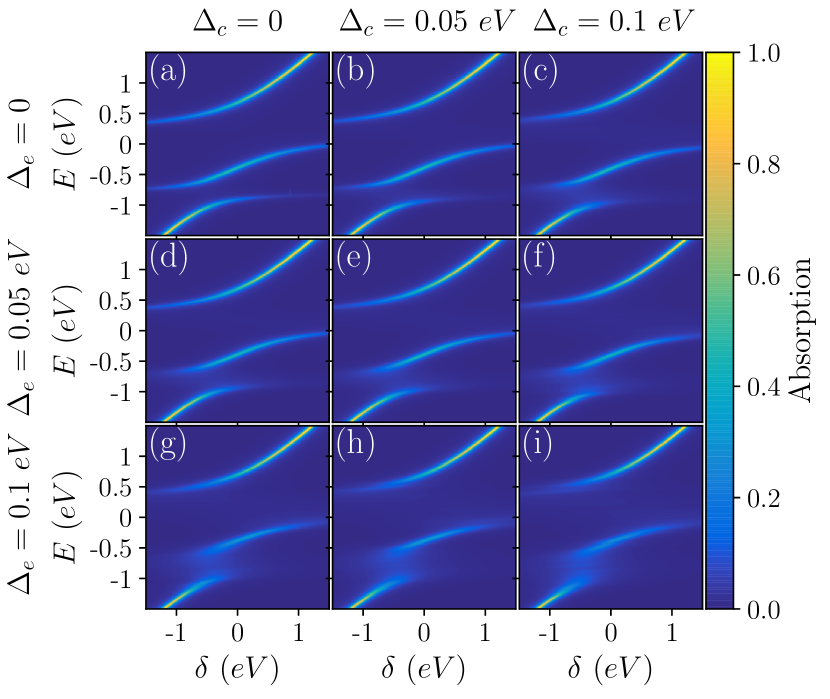
Figure 5: Effects of disorder in exciton energies and couplings on the optical absorption spectrum. Energies and couplings are taken randomly from gaussian distributions of widths $\Delta_{e}$ and $\Delta_{c}$ with mean values given by $\omega_{s}=0,\omega_{t}=-J=-0.5~{}eV$, and $\omega_{R}=0.5~{}eV,\lambda=0.3~{}eV$. $\Delta_{e}$ varies along the column whereas $\Delta_{c}$ varies along the rows, as labelled. Panel $(a)$ is the same as Fig. 4$(e)$. The results are obtained at $N=100$ and are averaged over $400$ independent random samples for the energies and couplings to reduce the noise due to a relatively small $N$. We see that the energetic disorder is relatively more detrimental but the spectrum keeps its main features intact even at the largest (and quite realistic) disorder strengths shown [panel $(i)$].

V Relaxation dynamics of the dark states

We know the basic difference between the generic weak and the strong coupling cases. In the former case, the stationary states are not much different from the original states, they acquire only a small component from each other that causes transitions between the original states usually relaxing the system towards the lower energy. (In the latter case, the stationary states are superpositions of the original states shifted in energies with sizable components from multiple original states.) Inter-system-crossing and reverse intersystem crossing are examples of the weak coupling in organic materials that is caused by a spin-orbit coupling $\lambda$ that is much smaller than the energetic difference $J$ between the singlet and the triplet exciton states and hence is assumed to couple them only weakly.

In the clean system we considered in Secs. II and III, the bright and the dark states are energetically separated. The bright states along with the cavity states make the polaritons while the dark states in the singlet and the triplet sector are completely decoupled from the bright sector. They make the dark bands or levels due to their intersector coupling.

We would like to explore how a disorder in the spin-orbit coupling affects this picture. We find that it can couple the bright singlet states to the dark triplet states and vice versa. This weak coupling will induce transitions between the dark bands and polaritons where the former contain the dark components and the latter the bright components. So we have a relaxation channel that can transfer the excitations from the dark bands to the polaritons.

To compute the transition rate between two states, we need to consider two quantities, the squared transition matrix element between them and the energy difference between them. If we are to compute the transition rate from a set of degenerate states to a given state, we can combine the squared transition matrix element for all states in the set. Since the dark bands should not be too wide, we can apply this idea here and combine the squared transition matrix elements to get a single number that can be used in the Fermi golden rule, or a more sophisticated formalism for an open quantum system involving the bath spectral density del Pino et al. (2015, 2018), to calculate the total transition rate.

It can be easily verified that for a degenerate manifold where multiple representations of the states are possible, the transition matrix elements squared for all states always sum up to a unique value and it is independent of the choice of the representation. We will continue using the same representation for the dark states that we introduced in sec. II.3 to compute this quantity.

V.1 Matrix elements

Let us calculate the matrix elements of the Hamiltonian $\mathcal{\hat{H}}_{\Delta}$ in Eq. 25 containing a disorder in the spin-orbit couplings only, i.e., $\Delta_{\lambda}>0$, but ${\Delta_{e}=0=\Delta_{\omega_{R}}}$.

$$\mathcal{H}_{{\mathcal{S}_{0}},{\mathcal{T}_{0}}} =\braket{{\mathcal{S}_{0}}}{\mathcal{\hat{H}}_{\Delta}}{{\mathcal{T}_{0}}},$$

$$=\frac{1}{N}\sum_{i=1}^{N}\lambda_{i}=\braket{\lambda}=\lambda,$$ (26)

where $\braket{\lambda}=\lambda$ is the mean value of the spin-orbit coupling. Defining,

$$\Lambda_{j} \equiv\left(\sum_{i=1}^{j}\lambda_{i}-j\lambda_{j+1}\right),$$ (27)

we can similarly write other nonzero matrix elements,

$$\mathcal{H}_{{\mathcal{S}_{0}},{\mathcal{T}_{j}}} =\frac{1}{\sqrt{Nj(j+1)}}\Lambda_{j}=\mathcal{H}_{{\mathcal{T}_{0}},{\mathcal{S}_{j}}},$$ (28)

$$\mathcal{H}_{{\mathcal{S}_{j}},{\mathcal{T}_{j^{\prime}>j}}} =\frac{1}{\sqrt{j(j+1)j^{\prime}(j^{\prime}+1)}}\Lambda_{j},$$ (29)

$$\mathcal{H}_{{\mathcal{S}_{j}},{\mathcal{T}_{j^{\prime}<j}}} =\frac{1}{\sqrt{j(j+1)j^{\prime}(j^{\prime}+1)}}\Lambda_{j^{\prime}},$$ (30)

$$\mathcal{H}_{{\mathcal{S}_{j}},{\mathcal{T}_{j}}} =\frac{1}{j(j+1)}\left(\sum_{i=1}^{j}\lambda_{i}+j^{2}\lambda_{j+1}\right).$$ (31)

We would like to compare the relative sizes of these matrix elements at large $N$. Using

$$\sum_{i=1}^{j}\lambda_{i}\to j\braket{\lambda}$$ (32)

introduces $\mathcal{O}(\Delta_{\lambda})$ errors at small $j$ but becomes exact at $j\gg 1$. At $N\to\infty$, states with $j,j^{\prime}\gg 1$ are dominant, for which we can approximate the matrix elements in Eqs. 28-31. Noting that

$$\Lambda_{j}\simeq j(\lambda-\lambda_{j+1})\approx j\mathcal{O}(\Delta_{\lambda}),$$ (33)

we obtain

$$\mathcal{H}_{{\mathcal{S}_{0}},{\mathcal{T}_{j}}} =\mathcal{H}_{{\mathcal{T}_{0}},{\mathcal{S}_{j}}}\approx\mathcal{O}(\Delta_{\lambda})/\sqrt{N},$$ (34)

$$\mathcal{H}_{{\mathcal{S}_{j}},{\mathcal{T}_{j^{\prime}>j}}} \approx\mathcal{O}(\Delta_{\lambda})/j,$$ (35)

$$\mathcal{H}_{{\mathcal{S}_{j}},{\mathcal{T}_{j^{\prime}<j}}} \approx\mathcal{O}(\Delta_{\lambda})/j^{\prime},$$ (36)

$$\mathcal{H}_{{\mathcal{S}_{j}},{\mathcal{T}_{j}}} \approx\lambda.$$ (37)

First, it is clear that the “off-diagonal” (${j\neq j^{\prime}}$) matrix elements in Eqs. 35 and 36 are suppressed by $j,j^{\prime}$ and so vanish quickly at $j,j^{\prime}\gg 1$ and can be ignored in comparison to the diagonal terms. The value of the off-diagonal term at the lowest $j,j^{\prime}=1,2$ is $(\lambda_{1}-\lambda_{2})/\sqrt{12}$ from exact expression, Eq. 29. Even substituting ${(\lambda_{1}-\lambda_{2})\to\Delta_{\lambda}}$, we obtain ${0.28\Delta_{\lambda}=0.028~{}eV}$ at $\Delta_{\lambda}=0.1~{}eV$, which is still an order of magnitude smaller than the diagonal term in Eq. 37 if ${\lambda\sim 0.3~{}eV}$. Furthermore, these off-diagonal terms are $\mathcal{O}(1/\sqrt{N})$ smaller than the coupling between the dark and the bright sector, Eq. 34, for most of the dark states (large $j$), so it is a fair approximation to ignore them. This leads to a great simplification as, treating Eq. 34 to be only a weak coupling, it makes the dark sector a sum of two-level systems (with modified couplings) that can be analytically solved.

Had we considered the Fourier representation for the dark states, ${\ket{{\mathcal{S}_{k}}}\to\sum_{n=1}^{N}e^{i2\pi kn/N}\sigma_{n}^{+}\ket{GS}}$, ${\ket{{\mathcal{T}_{k}}}\to\sum_{n=1}^{N}e^{i2\pi kn/N}\tau_{n}^{+}\ket{GS}}$, we would have obtained ${\mathcal{H}_{{\mathcal{S}_{0}},{\mathcal{T}_{j}}}=\mathcal{H}_{{\mathcal{S}_{l}},{\mathcal{T}_{j+l}}}}$ with ${j,l\in[1,N-1]}$, and it would not have been possible to ignore the off-diagonal couplings between the dark states in comparison to the couplings between the bright and the dark sector.

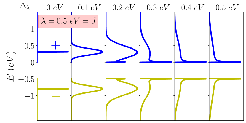
Figure 6: The evolution of the dark bands with the disorder in the spin-orbit couplings $\Delta_{\lambda}$. The density of states of $\pm$ dark bands is shown at $\lambda=0.5~{}eV=J$, for a set of $\Delta_{\lambda}$ values, $\Delta_{\lambda}=0-0.5~{}eV$ in steps of $0.1~{}eV$.

V.2 Dark bands

Assuming the polaritonic states are energetically away from the dark sectors, the coupling between the dark and the bright states, Eq. 34, will act only as a small perturbation at large $N$. For the diagonalization of the dark sectors, we can safely ignore it leaving only the diagonal terms (Eq. 31). So, the dark bands in the presence of disorder can be analytically calculated, given by,

$$\ket{\mathcal{D}_{j,\pm}} =A_{j,\pm}\ket{{\mathcal{S}_{j}}}\pm B_{j,\pm}\ket{{\mathcal{T}_{j}}},$$ (38)

$$E_{j,\pm} =\frac{1}{2}(-J\pm\sqrt{J^{2}+4\lambda_{jj}^{2}}),$$ (39)

$$A_{j,+} =\cos(\theta_{j}),A_{j,-}=\sin(\theta_{j}),B_{j,\pm}=A_{j,\mp},$$ (40)

$$2\theta_{j} =\tan^{-1}(2\lambda_{jj}/J),\lambda_{jj}\equiv\mathcal{H}_{{\mathcal{S}_{j}},{\mathcal{T}_{j}}}.$$ (41)

From hereon, we will refer to the two dark bands with their labels $\pm$. Figure 6 shows how the distribution of dark band energies $\{E_{j,\pm}\}$, i.e., the density of states for the dark bands $\pm$, evolve with $\Delta_{\lambda}$ at $\lambda=0.5~{}eV=J$. At $\Delta_{\lambda}=0$, the two bands are flat as expected but at a small finite $\Delta_{\lambda}$ become Gaussian. As $\Delta_{\lambda}$ increase, the distribution of molecular couplings $\lambda_{i}$ creates a distribution of dark state couplings $\lambda_{jj}$ with more and more states away from the mean coupling $\lambda$. The couplings at and around zero value increase in number so we obtain the dark bands containing more and more states closer to the bare singlet and triplet dark states. The same is true for higher couplings that spread the bands away from the corresponding bare state energies, i.e., $E_{j,-}$ are pushed below while $E_{j,+}$ are pushed upwards. In other words, a wider distribution of $\lambda_{i}$ and hence $\lambda_{jj}$ create a wider range of mixing between the bare states, some very close to the pure singlet or triplet and some very close to the maximal $50/50$ mixing.

V.3 Transitions between dark bands and polaritons

The Hamiltonian of the bright sector is the same as $\mathcal{\hat{H}}_{B}$ in Eq. 9 under the approximations made above where the coupling between the dark and the bright is assumed weak and ignored in the diagonalization. $\mathcal{\hat{H}}_{B}$ cannot be analytically solved for general parameters, but we can consider the general form of its eigenstates, given by

$$\ket{\Phi_{x}} =\alpha_{x}\ket{{\mathcal{S}_{0}}}+\beta_{x}\ket{{\mathcal{T}_{0}}}+\gamma_{x}\ket{1_{P}},$$ (42)

where ${x=LP_{\pm},UP}$.

We are interested to find the effects of the perturbation, Eq. 28, on the dynamics of these polaritons and the dark states in Eq. 38. To this end, the matrix elements of the perturbation between a given pair of states should give us the probability for the transition between them. Here, we like to compute ${\mathcal{M}_{j,\pm,x}}$ where,

$$\mathcal{M}_{j,\pm,x} =\braket{\mathcal{D}_{j,\pm}}{\mathcal{\hat{H}}_{\Delta}}{\Phi_{x}},$$ (43)

$$=\left(\pm B_{j,\pm}\alpha_{x}+A_{j,\pm}\beta_{x}\right)\mathcal{M}_{j},$$ (44)

where $\mathcal{M}_{j}=\mathcal{H}_{{\mathcal{S}_{0}},{\mathcal{T}_{j}}}=\mathcal{H}_{{\mathcal{T}_{0}},{\mathcal{S}_{j}}}$ is given by Eq. 28.

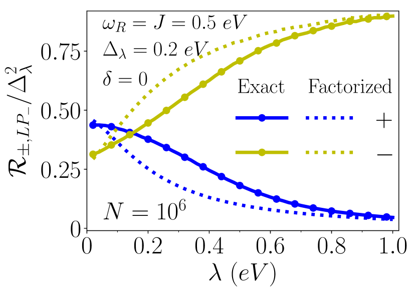
Figure 7: The relaxation of the dark states to $\ket{LP_{-}}$ induced by the disorder in the spin-orbit coupling. $\mathcal{R}_{\pm,LP_{-}}/\Delta_{\lambda}^{2}$ is shown as a function of $\lambda$ at $\delta=0$, $\omega_{R}=J=0.5~{}eV$. At $\lambda=0$, the dark states are either singlet or triplet so the interference term vanishes and $\mathcal{R}_{\pm,LP_{-}}$ are determined only by the weights of the corresponding bright components in $\ket{LP_{-}}$. As $\lambda$ increases, the dark states obtain the missing components and the interference between the two transition paths becomes important. $\mathcal{R}_{+,LP_{-}}$ ($\mathcal{R}_{-,LP_{-}}$) decreases (increases) due to destructive (constructive) interference. The factorised case overestimates the interference term.

V.4 Total squared matrix elements $\mathcal{R}_{\pm,x}$

Since the dark state should make a narrow band at typical parameters, their energy difference from a given polaritonic state is approximately the same. So to calculate the transition rate between the $+$ ($-$) dark band and polariton $\ket{\Phi_{x}}$, we can simply sum the corresponding squared matrix elements over all dark states $\{\ket{\mathcal{D}_{j,+}}\}$ ($\{\ket{\mathcal{D}_{j,-}}\}$).

$$\mathcal{R}_{\pm,x} =\sum_{j=1}^{N-1}|\mathcal{M}_{j,\pm,x}|^{2},$$

$$=\sum_{j=1}^{N-1}\left(B_{j,\pm}^{2}\alpha_{x}^{2}+A_{j,\pm}^{2}\beta_{x}^{2}+\mathcal{I}_{j,\pm,x}\right)\mathcal{M}_{j}^{2},$$ (45)

where

$$\mathcal{I}_{j,\pm,x} =\pm\alpha_{x}\beta_{x}\sin(2\theta_{j}),$$ (46)

gives the interference between the two transition paths available: from the dark singlet to the bright triplet and from the dark triplet to the bright singlet, in case of a transition from a given dark band ($\pm$) state to a polaritonic state. We will see below that this interference can suppress or enhance the relaxation rate quite substantially.

Equation 45 can be computed numerically, but it can also be approximated as follows. At ${\lambda\ll J}$, ${\mathcal{I}_{j,\pm,x}\sim 0}$ when ${A_{j,+},B_{j,-}\simeq 1}$, ${A_{j,-},B_{j,+}\simeq 0}$, and $\ket{\mathcal{D}_{j,+}}\simeq\ket{{\mathcal{S}_{j}}}$ and $\ket{\mathcal{D}_{j,-}}\simeq\ket{{\mathcal{T}_{j}}}$. Then, ${\mathcal{R}_{+,x}\simeq\beta_{x}^{2}\mathcal{R}}$ and ${\mathcal{R}_{-,x}\simeq\alpha_{x}^{2}\mathcal{R}}$, where

$$\mathcal{R} =\sum_{j=1}^{N-1}|\mathcal{M}_{j}|^{2}.$$ (47)

From numerical tests at large enough $N$, we find that not only $\mathcal{R}$ in Eq. 47 but also the distribution of the matrix elements $\mathcal{M}_{j}$ is independent of the mean coupling $\lambda$, they only depend on the disorder strength $\Delta_{\lambda}$. This means that, to see how $\mathcal{R}_{\pm,x}$ behave with $\lambda$ at a fixed $\Delta_{\lambda}$, we only need to focus on the distribution of the terms in the prefactor of $\mathcal{M}_{j}^{2}$ in Eq. 45.

V.5 Factorization and approximate expressions for $\mathcal{R}_{\pm,x}$

At ${\lambda\gtrsim J}$, we can approximate $\mathcal{R}_{\pm,x}$ by using the dark bands for the clean system in Eq. 12 instead of actual dark bands in Eq. 38. We will see that this turns out to be a reasonably good approximation. So the coefficients and the interference term in Eq. 45 are assumed to be the same for all states in a given dark band, i.e., ${A_{j,\pm}\to A_{\pm}}$, etc. It leads to a factorisation,

$$\mathcal{R}_{\pm,x} =\left(B_{\pm}^{2}\alpha_{x}^{2}+A_{\pm}^{2}\beta_{x}^{2}+\mathcal{I}_{\pm,x}\right)\mathcal{R}.$$ (48)

Thus, the problem reduces to the computation of the total squared matrix element $\mathcal{R}$ between the bright singlet and the whole dark triplet space (or vice versa) along with the diagonalization of a two-level dark and three-level polariton system to compute the prefactor in Eq. 48.

V.6 Numerical Results

Figure 7 presents the numerical results for the total squared matrix element between the dark bands $\pm$ and the lowest polaritonic state $\ket{LP_{-}}$. $\mathcal{R}_{\pm,LP_{-}}$ from Eq. 45 for $x=LP_{-}$ is shown as a function of $\lambda$ at ${\omega_{R}=J=0.5~{}eV}$, ${\delta=0,\Delta_{\lambda}=0.2~{}eV}$, and $N=10^{6}$. For comparison, the factorized version in Eq. 48 is also shown. The results are well converged with respect to the system size $N$. We note that the factorized results are reasonably good approximation. To understand the exact results, we will first look at the behavior of the factorized version and then see why the exact results differ.

We will see below that the factor $\mathcal{R}$ in Eq. 48 is essentially independent of $\lambda$ so the behavior of the factoried case as a function of $\lambda$ can be understood by looking at how the coefficients in the prefactor of $\mathcal{R}$ in Eq. 48, in particular, the interference term $\mathcal{I}_{\pm,x}$, change with $\lambda$. For $x=LP_{-}$, the coefficients $\alpha_{x},\beta_{x}$ have different signs (at $\lambda,\omega_{R}\geq 0$), so the interference term can be written as

$$\mathcal{I}_{\pm,x} =\mp|\alpha_{x}\beta_{x}|\sin(2\theta),$$

$$\propto\mp\sin(2\theta)=\mp\lambda/\sqrt{\lambda^{2}+(J/2)^{2}},$$

which means that the two paths will interfere constructively for the $-$ and destructively for the $+$ dark band.

As discussed before for the $\lambda\ll J$ limit, at small $\lambda\sim 0$ in Fig. 7, either component significantly dominates in the two dark bands (the singlet dominates in the $+$ band and the triplet dominates in the $-$ band), reducing the size of $\mathcal{I}_{\pm,x}$. So $\mathcal{R}_{\pm,LP_{-}}$ are determined primarily from the size of the bright exciton components in $\ket{LP_{-}}$. At the parameters considered in Fig. 7, the bright triplet component of $\ket{LP_{-}}$ is slightly larger than its bright singlet component, so the $+$ band with dark singlet character relaxes more quickly. That is, $\mathcal{R}_{+,LP_{-}}$ is slightly larger than $\mathcal{R}_{-,LP_{-}}$ at $\lambda\sim 0$. However, as $\lambda$ increases, the two bright exciton components in $\ket{LP_{-}}$ increase slightly but the $\pm$ dark bands acquire more and more mixed character, so the interference term quickly becomes more and more important, explaining the increase and decrease in $\mathcal{R}_{\pm,LP_{-}}$.

Compared to the exact results, the factorized version overestimates the interference effect. The reason is simple. A distribution in the couplings $\{\lambda_{i}\}$ creates a similar distribution for the matrix elements $\lambda_{jj}=\mathcal{H}_{{\mathcal{S}_{j}},{\mathcal{T}_{j}}}$ (see Fig. 10 in the tAppendix A), but it in turn creates a strongly distorted distribution for ${\sin(2\theta_{j})=\lambda_{jj}/\sqrt{\lambda_{jj}^{2}+(J/2)^{2}}}$ (that determines the interference term $\mathcal{I}_{j,\pm,x}$) that has lower average compared to the factorized model [${\sin(2\theta)=\lambda/\sqrt{\lambda^{2}+(J/2)^{2}}}$] at $\lambda>0$, with the difference first increasing (at $\lambda\lesssim J/2$) and then decreasing (at $\lambda\gtrsim J/2$) with an increase in $\lambda$. This is further discussed in the Appendix A where the distributions are also shown.

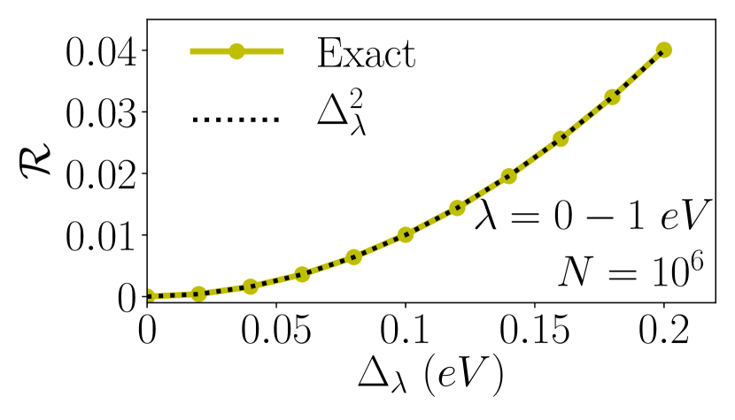
Figure 8: The squared matrix elements $\mathcal{R}$ that determines the transition rates between the dark states and polaritons as a function of the disorder in the spin-orbit coupling $\Delta_{\lambda}$. Analytical results $\mathcal{R}\simeq\Delta_{\lambda}^{2}$ also shown for comparison.

V.7 Analytical results for $\mathcal{R}$ at large $N$

Let us now consider the factor $\mathcal{R}$ in Eq. 48. At ${N\to\infty}$, an approximate but quite accurate expression for $\mathcal{R}$ can be obtained. Replacing

$$\sum_{i=1}^{j}\lambda_{i}\to j\braket{\lambda},$$ (49)

in Eq. 47 [with ${\mathcal{M}_{j}=\mathcal{H}_{{\mathcal{S}_{0}},{\mathcal{T}_{j}}}}$ in Eq. 28], where $\braket{\lambda}$ is the mean value of the spin-orbit coupling, introduces $\mathcal{O}(\Delta_{\lambda})$ errors at small $j$ but becomes exact at $j\gg 1$. With this approximation, we obtain

$$\mathcal{R} =\frac{1}{N}\sum_{j=1}^{N-1}\frac{j}{(j+1)}\left(\braket{\lambda}^{2}+\lambda_{j+1}^{2}-2\braket{\lambda}\lambda_{j+1}\right).$$ (50)

Again, replacing ${j/(j+1)\to 1}$ affects only a few terms with small $j\sim 1$, and should not affect the results in the thermodynamic limit, $N\to\infty$. Making this substitution in Eq. 50 and noting that

$$\sum_{j=1}^{N-1}\lambda_{j+1} =(N-1)\braket{\lambda},$$ (51)

$$\sum_{j=1}^{N-1}\lambda_{j+1}^{2} =(N-1)\braket{\lambda^{2}},$$ (52)

we obtain,

$$\mathcal{R} \simeq\frac{N-1}{N}\left(\braket{\lambda}^{2}+\braket{\lambda^{2}}-2\braket{\lambda}^{2}\right),$$

$$\simeq\left(\braket{\lambda^{2}}-\braket{\lambda}^{2}\right),$$

$$=\Delta_{\lambda}^{2}.$$ (53)

V.8 Comparison of analytical and numerical results for $\mathcal{R}$

Figure 8 shows the exact results for $\mathcal{R}$ at $N=10^{6}$, numerically computed from Eqs. 47 and 28, as well as the analytical expression, Eq. 53. The difference is invisible. The results also do not depend on $\lambda$, checked for ${\lambda=0-1~{}eV}$. It is worth reminding that the results do not depend on the explicit values of other parameters $\delta,\omega_{R}$, etc., as $\mathcal{R}$ is not the squared matrix element for the eigenstates but for the bright and dark states of different exciton types.

V.9 A simplified formula for $\mathcal{R}_{\pm,x}$

Using Eqs. 53 and 48, we obtain a very simple expression,

$$\mathcal{R}_{\pm,x} \simeq\left(B_{\pm}\alpha_{x}\pm A_{\pm}\beta_{x}\right)^{2}\Delta_{\lambda}^{2},$$ (54)

which can now be computed from the two dark (Eq. 12) and three polaritonic eigenstates, eliminating all complications. For the polaritonic states ${x=LP_{\pm}}$, we can even use the expressions obtained in sec. III.1.4, i.e., Eq. 23, which makes Eq. 54 an analytical expression. It can now be used with an appropriate open quantum system method to calculate, for instance, the population dynamics of the dark states and polaritons.

VI Summary and outlook

We investigate the role of the spin-orbit coupling between the singlet and the triplet molecular excitons in organic microcavities. We decouple the system into a bright sector that forms polaritons and a dark sector containing the dark exciton states that are decoupled from the cavity and form two dark bands. We show that the spin-orbit coupling splits the lower polariton into two branches that can be observed in the optical absorption spectrum. We find that when the cavity is in resonance with the triplet state, we obtain triplet polaritons. We also see the effects of disorder in energies and couplings on the absorption spectrum and see that the experiments should be able to find the spin-orbit induced splitting at typical disorder strengths. The spin-orbit coupling couples the bright singlet to the bright triplet and the dark singlet to the dark triplet sectors but does not couple the bright to the dark sectors. We show that the disorder in the spin-orbit coupling does exactly that and hence can be potentially very useful in optoelectronic devices where dark population is desired to be transferred to the polaritons. Considering it to be a weak coupling, we calculate the squared transition matrix elements between the dark bands and polaritons and also find approximate analytical expressions for them that can be employed to calculate the population dynamics.

There are plenty of organic molecules that have been proven to exhibit large enough spin-orbit coupling in electroluminescent devices where an efficient ISC along with a large radiative phosphorescent rate, or a large RISC rate in TADF, is observed. Some examples include heavy metal complexes Yersin et al. (2011) containing Ir, Pt, Os, Cu, Ag etc., such as PtOEP (platinum octaethylporphyrin) Baldo et al. (1998), Ir(ppy)₃, Btp₂Ir(acac), FIrpic  Kawamura et al. (2005), Pt(4,6-dFppy)(acac) and Ir(4,6-dFppy)₂(acac) Rausch et al. (2010), Ir(dm-2-piq)₂(acac), Cu(POP)(pz₂BH₂) Yersin et al. (2011), and mixed-ligand iradium complexes Ir(Phbib)(ppy)Cl, Ir(Mebib)(mppy)Cl, Ir(Mebib)(ppy)Cl, etc. Obara et al. (2006). Since these molecules are excellent at photoemission, they also have a large dipole matrix element required to achieve strong matter-light coupling, and thus are promising candidates to demonstrate the lower polariton splitting or an enhanced dark state to polariton relaxation as predicted in this work.

Besides the experimental scrutiny of our results, various unexplored avenues for future theoretical work also exist as described in the following. We know that the triplet exciton has a net spin and hence a magnetic moment, so $\ket{LP_{\pm}}$ would borrow it (proportional to the triplet weight) and should thus be manipulated using an external magnetic field. It would be interesting to consider all three triplet states in the model and explore the response of the system to such a field. When both the dark bands are able to relax to $\ket{LP_{-}}$, it can bring down the threshold pump power for creating their condensate or lasing. Considering it an open quantum system with an appropriate bath spectral density to study how the spin-orbit coupling and its disorder affect this threshold is intriguing. Due to the polaron decoupling at large $N$, we ignored the vibrations and vibronic coupling in our model. Exploring the interplay between vibrations and spin-orbit coupling at small $N$ can also be a future work.

*

Appendix A SUPPRESSION OF THE INTERFERENCE BETWEEN THE TWO TRANSITION PATHS DUE TO DISORDER

Figure 9: (Color online) An illustration of how a distribution of $\lambda_{jj}$ is mapped onto a distribution of $\sin(2\theta_{j})$. The number of entries in the $\lambda_{jj}$ in the yellow (gray) shaded region go to the blue (black) slot in the $\sin(2\theta_{j})$ distribution. The entries on the right of the yellow (gray) shaded region in the $\lambda_{jj}$ distribution shown or in any other distribution that we consider (where $\lambda>0$) all go to the narrow region above the blue (black) shaded region below the thick black dotted curve.

First, let us understand how a distribution of couplings $\lambda_{jj}$ transforms into a distribution of the interference terms, $\sin(2\theta_{j})$. Figure 9 shows a $\lambda_{jj}$ distribution that is centered around zero along with the function $\sin(2\theta_{j})$. The number of elements in the $\lambda_{jj}$ distribution in a window $0.2~{}eV>\lambda_{jj}>0.3~{}eV$ [yellow (gray) shaded region] will move to the blue (black) shaded region on the $\sin(2\theta_{j})$ distribution that is shown on the right. The elements at $\lambda_{jj}>0.5~{}eV$ are very few in this distribution but can be half of the total for a distribution with $\lambda\sim 0.5~{}eV$. Following the above rule, they all move to a very narrow region close to the extreme value of $\sin(2\theta_{j})=1$ making a sharp peaked distribution there. The entries close to ${\lambda_{jj}=0}$ will spread over a larger region on the ${\sin(2\theta_{j})}$ distribution because it has a sharp change around $\lambda_{jj}=0$, dispersing the distribution shown here (with mean at ${\lambda=0}$) symmetrically on either side but creating a long tail for slightly shifted distributions. This is seen in Fig. 10, where the distributions of $\lambda_{jj}$ and ${\sin(2\theta_{j})}$ are shown at ${N=10^{6}}$, ${\Delta_{\lambda}=0.2~{}eV}$, ${J=0.5~{}eV}$ and a set of $\lambda$ values, ${\lambda=0,0.25,0.5,and0.75~{}eV}$. The mean value of the distribution and the value for the factorized case (that is equivalent to assuming no disorder in $\lambda_{i}$), Eq. 48, are also shown by solid and dotted vertical lines.

As explained using Fig. 9, compared to the input distributions $\lambda_{jj}$, the distributions of ${\sin(2\theta_{j})}$ are spread more near zero but shifted more away from zero, resulting in flattened and broadened distribution at $\lambda=0$ (red), but creating a long tail at $\lambda=0.25~{}eV$ and pushing the whole distributions at $\lambda=0.5and0.75~{}eV$ close to $1$ on the ${\sin(2\theta_{j})}$ scale. The asymmetry introduced lowers the mean value for the distributions (solid vertical lines) from the factorized case (dotted vertical lines) for all $\lambda>0$ cases shown, with the difference decreasing at higher $\lambda$.

We can now understand that at $0<\lambda<J/2=0.25~{}eV$ (distributions not shown), the difference keeps increasing with an increase in $\lambda$. This increase and decrease of the difference between the exact and the factorize case is reflected in Fig. 7, and shows that the interference is, on average, suppressed by the disorder in the couplings and the suppression is maximum around $\lambda=J/2$. The reason that the factorized model overestimates the interference effect in Fig. 7 is that it ignores this suppression.

Figure 10: (Color online) The influence of the distribution of couplings $\{\lambda_{i}\}$ on the couplings between the dark states $\lambda_{jj}$ and the interference terms $\sin(2\theta_{j})$. The distributions are calculated at $N=10^{6}$, $\Delta_{\lambda}=0.2~{}eV$ and $J=0.5~{}eV$ for $\lambda=0,0.25,0.5,0.75~{}eV$ with line colour changing from yellow to blue (gray to black). The distributions are normalised by their peak value for easier comparison. Solid and dotted vertical lines show the mean value of the distribution and the value for the factorised case, Eq. 48. (a) The distributions of the matrix elements between the singlet and the triplet dark states $\lambda_{jj}$. The distributions do not seem to differ much from the original gaussians for $\{\lambda_{i}\}$ (not shown here). The thick dotted curve shows the dependence of the interference term ${\sin(2\theta_{j})}$ on $\lambda_{jj}$—the values are shown on the vertical axis on the right side as indicated by a small arrow. (b) The distributions of $\sin(2\theta_{jj})$ corresponding to the distributions of $\lambda_{jj}$ shown in (a). The mean value for the distributions (solid vertical lines) is lower from that of the factorised case (dotted vertical lines) at $\lambda\geq 0.25~{}eV$ but the difference decreases with an increase (or decrease, see text) in $\lambda$.

References

- Lidzey et al. (1998) D. G. Lidzey, D. Bradley, M. Skolnick, T. Virgili, S. Walker, and D. Whittaker, Nature 395, 53 (1998).
- Kasprzak et al. (2006) J. Kasprzak, M. Richard, S. Kundermann, A. Baas, P. Jeambrun, J. M. J. Keeling, F. M. Marchetti, M. H. Szymańska, R. André, J. L. Staehli, V. Savona, P. B. Littlewood, B. Deveaud, and L. S. Dang, Nature 443, 409 (2006).
- Keeling and Kéna-Cohen (2020) J. Keeling and S. Kéna-Cohen, Ann. Rev. Phys. Chem. 71 (2020), 10.1146/annurev-physchem-010920-102509.
- Mitrano et al. (2016) M. Mitrano, A. Cantaluppi, D. Nicoletti, S. Kaiser, A. Perucchi, S. Lupi, P. Di Pietro, D. Pontiroli, M. Riccò, S. R. Clark, D. Jaksch, and A. Cavalleri, Nature 530, 461 (2016).
- Schlawin et al. (2017) F. Schlawin, A. S. D. Dietrich, M. Kiffner, A. Cavalleri, and D. Jaksch, Phys. Rev. B 96, 064526 (2017).
- Feist and Garcia-Vidal (2015) J. Feist and F. J. Garcia-Vidal, Phys. Rev. Lett. 114, 196402 (2015).
- Hagenmüller et al. (2017) D. Hagenmüller, J. Schachenmayer, S. Schütz, C. Genes, and G. Pupillo, Phys. Rev. Lett. 119, 223601 (2017).
- Schäfer et al. (2019) C. Schäfer, M. Ruggenthaler, H. Appel, and A. Rubio, Proc. Natl. Acad. Sci. U. S. A. 116, 4883 (2019).
- Zeb et al. (2020) M. A. Zeb, P. G. Kirton, and J. Keeling, “Incoherent charge transport in an organic polariton condensate,” (2020), arXiv:2004.09790 [cond-mat.quant-gas] .
- Thomas et al. (2019) A. Thomas, L. Lethuillier-Karl, K. Nagarajan, R. M. A. Vergauwe, J. George, T. Chervy, A. Shalabney, E. Devaux, C. Genet, J. Moran, and T. W. Ebbesen, Science 363, 615 (2019).
- Herrera and Spano (2016) F. Herrera and F. C. Spano, Phys. Rev. Lett. 116, 238301 (2016).
- Galego et al. (2016) J. Galego, F. J. Garcia-Vidal, and J. Feist, Nat. Commun. 7, 13841 (2016).
- Galego et al. (2017) J. Galego, F. J. Garcia-Vidal, and J. Feist, Phys. Rev. Lett. 119, 136001 (2017).
- Martínez-Martínez et al. (2018) L. A. Martínez-Martínez, R. F. Ribeiro, J. Campos-González-Angulo, and J. Yuen-Zhou, ACS Photonics 5, 167 (2018).
- Ebbesen (2016) T. W. Ebbesen, Acc. Chem. Res 49, 2403 (2016).
- Feist et al. (2017) J. Feist, J. Galego, and F. J. Garcia-Vidal, ACS Photonics 5, 205 (2017).
- Ribeiro et al. (2018) R. F. Ribeiro, L. A. Martínez-Martínez, M. Du, J. Campos-Gonzalez-Angulo, and J. Yuen-Zhou, Chem. Sci. 9, 6325 (2018).
- Nazir and McCutcheon (2016) A. Nazir and D. P. S. McCutcheon, Journal of Physics: Condensed Matter 28, 103002 (2016).
- Polak et al. (2020) D. Polak, R. Jayaprakash, T. P. Lyons, L. A. Martínez-Martínez, A. Leventis, K. J. Fallon, H. Coulthard, D. G. Bossanyi, K. Georgiou, A. J. Petty, II, J. Anthony, H. Bronstein, J. Yuen-Zhou, A. I. Tartakovskii, J. Clark, and A. J. Musser, Chem. Sci. 11, 343 (2020).
- Dias et al. (2013) F. B. Dias, K. N. Bourdakos, V. Jankus, K. C. Moss, K. T. Kamtekar, V. Bhalla, J. Santos, M. R. Bryce, and A. P. Monkman, Advanced Materials 25, 3707 (2013), https://onlinelibrary.wiley.com/doi/pdf/10.1002/adma.201300753 .
- Kaji et al. (2015) H. Kaji, H. Suzuki, T. Fukushima, K. Shizu, K. Suzuki, S. Kubo, T. Komino, H. Oiwa, F. Suzuki, A. Wakamiya, Y. Murata, and C. Adachi, Nature Communications 6, 8476 (2015).
- Wong and Zysman-Colman (2017) M. Y. Wong and E. Zysman-Colman, Advanced Materials 29, 1605444 (2017), https://onlinelibrary.wiley.com/doi/pdf/10.1002/adma.201605444 .
- Yin et al. (2020) X. Yin, Y. He, X. Wang, Z. Wu, E. Pang, J. Xu, and J.-a. Wang, Frontiers in Chemistry 8, 725 (2020).
- Eizner et al. (2019) E. Eizner, L. A. Martínez-Martínez, J. Yuen-Zhou, and S. Kéna-Cohen, Science Advances 5 (2019), 10.1126/sciadv.aax4482, https://advances.sciencemag.org/content/5/12/eaax4482.full.pdf .
- Yu et al. (2021) Y. Yu, S. Mallick, M. Wang, and K. Börjesson, Nature Communications 12, 3255 (2021).
- Baldo et al. (1998) M. A. Baldo, D. F. O’Brien, Y. You, A. Shoustikov, S. Sibley, M. E. Thompson, and S. R. Forrest, Nature 395, 151 (1998).
- Adachi et al. (2001) C. Adachi, M. A. Baldo, M. E. Thompson, and S. R. Forrest, Journal of Applied Physics 90, 5048 (2001), https://doi.org/10.1063/1.1409582 .
- Kawamura et al. (2005) Y. Kawamura, K. Goushi, J. Brooks, J. J. Brown, H. Sasabe, and C. Adachi, Applied Physics Letters 86, 071104 (2005), https://aip.scitation.org/doi/pdf/10.1063/1.1862777 .
- Yersin et al. (2011) H. Yersin, A. F. Rausch, R. Czerwieniec, T. Hofbeck, and T. Fischer, Coordination Chemistry Reviews 255, 2622 (2011), controlling photophysical properties of metal complexes: Towards molecular photonics.
- Martínez-Martínez et al. (2019) L. A. Martínez-Martínez, E. Eizner, S. Kéna-Cohen, and J. Yuen-Zhou, The Journal of Chemical Physics 151, 054106 (2019), https://doi.org/10.1063/1.5100192 .
- Agranovich et al. (2002) V. Agranovich, M. Litinskaia, and D. Lidzey, physica status solidi (b) 234, 130 (2002).
- Agranovich et al. (2003) V. M. Agranovich, M. Litinskaia, and D. G. Lidzey, Phys. Rev. B 67, 085311 (2003).
- Litinskaya et al. (2004) M. Litinskaya, P. Reineker, and V. Agranovich, Journal of Luminescence 110, 364 (2004).
- Michetti et al. (2009) P. Michetti, G. La Rocca, and G. C. L. Rocca, Phys. Rev. B 79, 035325 (2009).
- del Pino et al. (2018) J. del Pino, F. A. Y. N. Schröder, A. W. Chin, J. Feist, and F. J. Garcia-Vidal, Phys. Rev. Lett. 121, 227401 (2018).
- Groenhof et al. (2019) G. Groenhof, C. Climent, J. Feist, D. Morozov, and J. J. Toppari, The Journal of Physical Chemistry Letters 10, 5476 (2019), pMID: 31453696, https://doi.org/10.1021/acs.jpclett.9b02192 .
- Sommer et al. (2021) C. Sommer, M. Reitz, F. Mineo, and C. Genes, Phys. Rev. Research 3, 033141 (2021).
- Mewes et al. (2020) L. Mewes, M. Wang, R. A. Ingle, K. Börjesson, and M. Chergui, Communications Physics 3, 157 (2020).
- Wers’́all et al. (2019) M. Wers’́all, B. Munkhbat, D. G. Baranov, F. Herrera, J. Cao, T. J. Antosiewicz, and T. Shegai, ACS Photonics 6, 2570 (2019), https://doi.org/10.1021/acsphotonics.9b01079 .
- Xiang et al. (2019) B. Xiang, R. F. Ribeiro, L. Chen, J. Wang, M. Du, J. Yuen-Zhou, and W. Xiong, The Journal of Physical Chemistry A 123, 5918 (2019), pMID: 31268708, https://doi.org/10.1021/acs.jpca.9b04601 .
- Tavis and Cummings (1968) M. Tavis and F. W. Cummings, Phys. Rev. 170, 379 (1968).
- Houdré et al. (1996) R. Houdré, R. P. Stanley, and M. Ilegems, Phys. Rev. A 53, 2711 (1996).
- Ćwik et al. (2016) J. A. Ćwik, P. Kirton, S. De Liberato, and J. Keeling, Phys. Rev. A 93, 033840 (2016).
- Dimitrov et al. (2016) S. D. Dimitrov, B. C. Schroeder, C. B. Nielsen, H. Bronstein, Z. Fei, I. McCulloch, M. Heeney, and J. R. Durrant, Polymers 8 (2016), 10.3390/polym8010014.
- Skolnick et al. (1998) M. S. Skolnick, T. A. Fisher, and D. M. Whittaker, Semiconductor Science and Technology 13, 645 (1998).
- Scully and Zubairy (1997) M. O. Scully and M. S. Zubairy, Quantum Optics (Cambridge University Press, 1997).
- Zeb et al. (2017) M. A. Zeb, P. Kirton, and J. Keeling, ACS Photonics 5, 249 (2017).
- Brion et al. (2007) E. Brion, L. H. Pedersen, and K. Mølmer, Journal of Physics A: Mathematical and Theoretical 40, 1033 (2007).
- Bässler (1981) H. Bässler, physica status solidi (b) 107, 9 (1981), https://onlinelibrary.wiley.com/doi/pdf/10.1002/pssb.2221070102 .
- Bässler et al. (1982) H. Bässler, G. Schönherr, M. Abkowitz, and D. M. Pai, Phys. Rev. B 26, 3105 (1982).
- del Pino et al. (2015) J. del Pino, J. Feist, and F. J. Garcia-Vidal, New J. Phys. 17, 053040 (2015).
- Rausch et al. (2010) A. F. Rausch, H. H. H. Homeier, and H. Yersin, “Organometallic Pt(II) and Ir(III) triplet emitters for oled applications and the role of spin–orbit coupling: A study based on high-resolution optical spectroscopy,” in Photophysics of Organometallics, edited by A. J. Lees (Springer Berlin Heidelberg, Berlin, Heidelberg, 2010) pp. 193–235.
- Obara et al. (2006) S. Obara, M. Itabashi, F. Okuda, S. Tamaki, Y. Tanabe, Y. Ishii, K. Nozaki, and M.-a. Haga, Inorganic Chemistry 45, 8907 (2006).