Burling graphs revisited, part I:
New characterizations

Abstract

The Burling sequence is a sequence of triangle-free graphs of increasing chromatic number. Each of them is isomorphic to the intersection graph of a set of axis-parallel boxes in $\mathbb{R}^{3}$. These graphs were also proved to have other geometrical representations: intersection graphs of line segments in the plane, and intersection graphs of frames, where a frame is the boundary of an axis-aligned rectangle in the plane.

We call Burling graph every graph that is an induced subgraph of some graph in the Burling sequence. We give five new equivalent ways to define Burling graphs. Three of them are geometrical, one is of a more graph-theoretical flavor, and one, that we call abstract Burling graphs, is more axiomatic.

Keywords: Burling graphs, intersection graphs of geometric objects

1 Introduction

Graphs in this paper have neither loops nor multiple edges. In this introduction they are non-oriented, but oriented graphs will be considered in the rest of the paper. A class of graphs is hereditary if it is closed under taking induced subgraphs. A triangle in a graph is a set of three pairwise adjacent vertices, and a graph is triangle-free if it contains no triangle. The intersection graph of sets $S_{1},\dots,S_{n}$ is defined as follows: the vertices are the sets, and for $i\neq j$, $S_{i}$ is connected to $S_{j}$ by an edge if and only if $S_{i}\cap S_{j}\neq\varnothing$.

Burling graphs

In 1965, Burling [2] proved that triangle-free intersection graphs of axis-aligned boxes in $\mathbb{R}^{3}$ have unbounded chromatic number. The work of Burling uses purely geometric terminology. However, one may rephrase it into a more modern graph theoretic setting and define in a combinatorial way a sequence of triangle-free graphs with increasing chromatic number, and prove that each of them is isomorphic to the intersection graph of a set of axis-parallel boxes in $\mathbb{R}^{3}$. The definition of this sequence is recalled in Section 4, and we call it the Burling sequence.

It was later proved that every graph in the Burling sequence is isomorphic to the intersection graph of various geometrical objects. In a work of Pawlik, Kozik, Krawczyk, Lason, Micek, Trotter and Walczak [7], the objects under consideration are line segments in the plane. The intersection graphs of line segments in the plane are called line segment graphs. In fact, the Burling sequence was rediscovered in [7], and the way it is presented in recent works is inspired by this paper.

In works of Pawlik, Kozik, Krawczyk, Lason, Micek, Trotter and Walczak [6], Krawczyk, Pawlik and Walczak [5], and later Chalopin, Esperet, Li and Ossona de Mendez [3], the objects under consideration are frames, where a frame is the boundary of an axis-aligned rectangle in the plane. In fact, a stronger result is given in [5]: it is proved that every graph of the Burling sequence is a restricted frame graph, meaning that the frames satisfy several constraints that we recall in Section 6.

The Burling sequence also attracted attention lately because it is a good source of examples of graphs of high chromatic number in some hereditary classes of graphs that are not defined geometrically, but by excluding several patterns as induced subgraphs. Most notably, it is proved in [7] that they provide a counter-example to a well-studied conjecture of Scott, see [11] for a survey.

Since graphs of the Burling sequence appear in the context of hereditary classes of graphs, it is natural to define Burling graphs as graphs that are induced subgraphs of some graph in the Burling sequence. Observe that Burling graphs trivially form a hereditary class (in fact, the smallest hereditary class that contains the Burling sequence). The goal of this work is a better understanding of Burling graphs.

New geometrical characterizations

In this first part, we give three new characterizations of Burling graphs: as intersection graphs of frames, as intersection graphs of line segments in the plane and as intersection graphs of boxes of the 3-dimensional space. The new feature of our characterizations is that they provide the following equivalences. We put some restrictions on the geometrical objects, to obtain what we call strict frame graphs, strict line segment graphs and strict box graphs. The precise definitions are given in Section 6. We then prove that a graph $G$ is a Burling graph if and only if it is a strict frame graph (resp. a strict line segment graph, a strict box graph).

Observe that in [7] (resp. [3, 6, 7]), it is proved that every Burling graph is a strict line segment graph (resp. a strict frame graph). The proofs there are implicit because the authors of these works do not mention our new restrictions, but it is straightforward to check that their way to embed Burling graphs in the plane satisfies them. Note that as pointed out by an anonymous referee, strict frame graphs are implicitly defined in [5] as intersection graphs of clean directed families of frames avoiding some configurations. Our contribution is the definition of the new restrictions on the geometrical objects and the converse statements: every strict frame graph and every strict line segment graph is a Burling graph. Examples of line segment graphs that are not Burling graphs are already given in [3]. We go further by providing examples of restricted frame graphs that are not Burling graphs, showing that our new restrictions are necessary, see Figures 15, 15 and 15. Note that proving that the examples are not Burling graphs is non-trivial and postponed to the second part of this work [9].

Combinatorial characterizations

The definition of Burling graphs as induced subgraphs of graphs in the Burling sequence is not very easy to handle, at least for us. So, to prove the equivalence between Burling graphs and our geometrical constructions, we have to introduce two other new equivalent definitions of Burling graphs. The first one, called derived graphs, is purely combinatorial: we see how every Burling graph can be derived from some tree structure using several simple rules (and we prove that only Burling graphs are obtained). Derived graphs are defined in Section 3 and their equivalence with Burling graphs is proved in Section 4. In fact, derived graphs have a natural orientation that is very useful to consider, so they are defined as oriented graphs. Then, in Section 5 we prove that derived graphs can be defined as graphs obtained from a set with two relations satisfying a small number of axioms, again with simple rules. We call these abstract Burling graphs.

The advantage of this approach is that derived graphs seem to be specific and well structured, while abstract Burling graphs seem to be general (though they are equivalent). As a consequence, derived graphs turn out to be useful to study the structure of Burling graphs, and this will be mostly done in the second part of this work [9]. On the other hand, since abstract Burling graphs are “general”, it is easy to check that geometrical objects satisfy the axioms in their definition. So the proof that every graph arising from one of our geometrical characterizations is an abstract Burling graph, and therefore a Burling graph, is not too long. This is done in Section 6. Moreover, abstract Burling graphs might be of use to prove other geometrical or combinatorial characterizations of Burling graphs.

Figure 1: The six equivalent classes of graphs in this article. Each arrow shows an inclusion and the label of the arrow shows where the proof may be found.

Sum up

To sum up, we have now six different ways to define Burling graphs: as induced subgraphs of graphs in the classical Burling sequence, as derived graphs, as abstract Burling graphs, as strict frame graphs, as strict line segment graphs and as strict box graphs. In Figure 1, we sum up where the different steps of the proofs of the equivalence between all classes can be found.

The second [9] and third [10] parts of this work are about the structure of Burling graphs and are motivated by the chromatic number in hereditary classes of graphs. For instance, we prove a decomposition theorem for oriented Burling graphs and study under what conditions simple operations such as gluing along a clique, subdividing an edge or contracting an edge preserve being a Burling graph. We prove that no subdivision of $K_{5}$ is a Burling graph. Moreover, we classify as Burling or not Burling many series-parallel graphs.

We also prove that no wheel is a Burling graph, where a wheel is a graph made of a chordless cycle and a vertex with at least three neighbors in the cycle. This last result was already known by Scott and Seymour (personal communication, 2017). Very recently, Davies rediscovered this independently and published a proof [4]. Some of the results of Part 2 and Part 3 appeared in the master thesis of the first author, see [8].

2 Notation

There is a difficulty regarding notations in this paper. The graphs we are interested in will be defined from trees. More specifically, a tree $T$ is considered and a graph $G$ is derived from it, following some rules defined in the next section. We have $V(G)=V(T)$ but $E(G)$ and $E(T)$ are different (disjoint, in fact). Also, even if we are originally motivated by non-oriented graphs, it turns out that $G$ has a natural orientation, and considering this orientation is essential in many of our proofs.

So, in many situations, we have to deal simultaneously with the tree, the oriented graph derived from it and the underlying graph of this oriented graph. A last difficulty is that since we are interested in hereditary classes, we allow removing vertices from $G$. However, we have to keep all vertices of $T$ to study $G$ because of the so-called shadow vertices: the vertices of $T$ that are not in $G$, which nevertheless capture essential structural properties of $G$. All this will become clearer in the next section. For now, it explains why we need to be very careful about the notation that is mostly classical, see [1].

Notation for trees

A tree is a graph $T$ such that for every pair of vertices $u,v\in V(T)$, there exists a unique path from $u$ to $v$. A rooted tree is a pair $(T,r)$ such that $T$ is a tree and $r\in V(T)$. The vertex $r$ is called the root of $(T,r)$. Often, the rooted tree $(T,r)$ is abusively referred to as $T$, in particular when $r$ is clear from the context.

In a rooted tree, each vertex $v$ except the root has a unique parent which is the neighbor of $v$ in the unique path from the root to $v$. We denote the parent of $v$ by $p(v)$. If $u$ is the parent of $v$, then $v$ is a child of $u$. A leaf of a rooted tree is a vertex that has no children. Note that every tree has at least one leaf. We denote by $L(T)$ the set of all leaves of $T$.

A branch in a rooted tree is a path $v_{1}v_{2}\dots v_{k}$ such that for each $i\in\{1,\dots,k-1\}$, the vertex $v_{i}$ is the parent of $v_{i+1}$. This branch starts at $v_{1}$ and finishes at $v_{k}$. A branch that starts at the root and finishes at a leaf is a principal branch. Note that every rooted tree has at least one principal branch.

If $T$ is a rooted tree, the descendants of a vertex $v$ are all the vertices that are on a branch starting at $v$. The ancestors of $v$ are the vertices on the unique path from $v$ to the root of $T$. Notice that a vertex is a descendant and an ancestor of itself. Any descendant of a vertex $v$, other than itself, is called a proper descendant of $v$.

It is classical to orient the edges of a rooted tree (from the root, or sometimes to the root), but to avoid any confusion with the oriented graph derived from a tree, we will not use any of these orientations here. Also, we will no more use words such as neighbors, adjacent, path, etc. for trees. Only parent, child, branch, descendant and ancestor will be used.

Notation for graphs and oriented graphs

By graph, we mean a non-oriented graph with no loops and no multiple edges. By oriented graph, we mean a graph whose edges (called arcs) are all oriented, and no arc is oriented in both directions. When $G$ is a graph or an oriented graph, we denote by $V(G)$ its vertex set. We denote by $E(G)$ the set of edges of a graph $G$ and by $A(G)$ the set of arcs of an oriented graph $G$. When $u$ and $v$ are vertices, we use the same notation $uv$ to denote an edge and an arc. However, observe that the arc $uv$ is different from the arc $vu$, while the edge $uv$ is equal to the edge $vu$.

For an oriented graph $G$, its underlying graph is the graph $H$ such that $V(H)=V(G)$ and for all $u,v\in V(H)$, $uv\in E(H)$ if and only if $uv\in A(G)$ or $vu\in A(G)$. We then also say that $G$ is an orientation of $H$. When there is no risk of confusion, we often use the same letter to denote an oriented graph and its underlying graph.

In the context of oriented graphs, we use the words in-neighbor, out-neighbor, in-degree, out-degree, sink and source with their classical meaning. Terms from the non-oriented realm, such as degree, neighbor, isolated vertex or connected component, when applied to an oriented graph, implicitly apply to its underlying graph.

Notation for binary relations

Let $S$ be a set, and let $\operatorname{R}$ be a binary relation on $S$. We write $x\operatorname{R}y$ for $(x,y)\in\operatorname{R}$, and $x\operatorname{\cancel{\operatorname{R}}}y$ for $(x,y)\notin\operatorname{R}$. For an element $s\in S$, we denote by $[s\operatorname{R}]$ the set $\{t\in S:s\operatorname{R}t\}$.

The relation $\operatorname{R}$ is asymmetric if for all $x,y\in S$, $x\operatorname{R}y$ implies $y\operatorname{\cancel{\operatorname{R}}}x$, and it is transitive if for all $x,y,z\in S$, $x\operatorname{R}y$ and $y\operatorname{R}z$ implies $x\operatorname{R}z$. The relation $\operatorname{R}$ is a strict partial order if it is asymmetric and transitive.

A directed cycle in $\operatorname{R}$ is a set of elements $x_{1},x_{2},\dots,x_{n}$, with $n\in\mathbb{N}$, such that $x_{1}\operatorname{R}x_{2}$, $x_{2}\operatorname{R}x_{3}$, $\dots$, $x_{n}\operatorname{R}x_{1}$. Note that when we deal with relations, we allow cycles on one or two elements. So, strict partial orders do not have directed cycles. In fact, a relation $\operatorname{R}$ has no directed cycles if and only if its transitive closure is a strict partial order.

An element $s\in S$ is said to be a minimal element with respect to $\operatorname{R}$ if there exists no element $t\in S\setminus\{s\}$ such that $t\operatorname{R}s$. Notice that if a relation $\operatorname{R}$ on a finite set $S$ has no directed cycle, then $S$ necessarily has a minimal element with respect to $\operatorname{R}$.

3 Derived graphs

In this section, we introduce the class of derived graphs and study some of their basic properties. A Burling tree is a 4-tuple $(T,r,\operatorname{\ell},\operatorname{c})$ in which:

1. $T$ is a rooted tree and $r$ is its root,

2. $\operatorname{\ell}$ is a function associating to each vertex $v$ of $T$ which is not a leaf, one child of $v$ which is called the last-born of $v$,

3. $\operatorname{c}$ is a function defined on the vertices of $T$. If $v$ is a non-last-born vertex in $T$ other than the root, then $\operatorname{c}$ associates to $v$ the vertex-set of a (possibly empty) branch in $T$ starting at the last-born of $p(v)$. If $v$ is a last-born or the root of $T$, then we define $\operatorname{c}(v)=\varnothing$. We call $\operatorname{c}$ the choose function of $T$.

By abuse of notation, we often use $T$ to denote the 4-tuple.

The oriented graph $G$ fully derived from the Burling tree $T$ is the oriented graph whose vertex-set is $V(T)$ and $uv\in A(G)$ if and only if $v$ is a vertex in $\operatorname{c}(u)$. A non-oriented graph $G$ is fully derived from $T$ if it is the underlying graph of the oriented graph fully derived from $T$.

A graph (resp. oriented graph) $G$ is derived from a Burling tree $T$ if it is an induced subgraph of a graph (resp. oriented graph) fully derived from $T$. The oriented or non-oriented graph $G$ is called a derived graph if there exists a Burling tree $T$ such that $G$ is derived from $T$.

Observe that if the root of $T$ is in $V(G)$, then it is an isolated vertex of $G$. Observe that a last-born vertex of $T$ that is in $G$ is a sink of $G$.

Let us give some examples. In all figures in this paper, the tree $T$ is represented with black edges while the arcs of $G$ are represented in red. The last-born of a vertex of $T$ is presented as its rightmost child. Moreover, shadow vertices, the vertices of $T$ that are not in $G$, are represented in white.

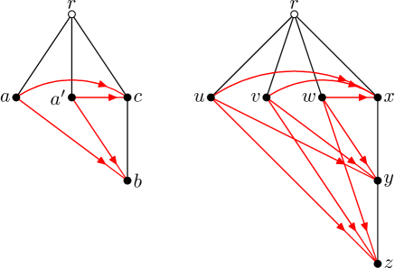
Figure 2: Complete bipartite graphs seen as derived graphs

On the first graph represented in Figure 2, $\operatorname{c}(x)=\operatorname{c}(y)=\{z,w\}$. It shows that at least one orientation of $C_{4}$ is a derived graph, so that $C_{4}$ is a derived graph. The second graph shows that $K_{3,3}$ is a derived graph, and it is easy to generalize this construction to $K_{n,m}$ for all integers $n,m\geq 1$. In both graphs, the vertex $r$ of $T$ is not a vertex of $G$. Figure 3 is a presentation of $C_{6}$ as a derived graph. Notice that, in this presentation, $v$ is a shadow vertex.

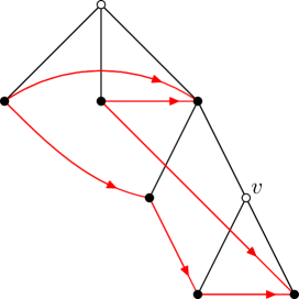
Figure 3: Cycle of length 6 seen as a derived graph

Notice that if a graph $G$ is derived from $T$, the branches of $T$, restricted to the vertices of $G$, are stable sets of $G$. In particular, no edge of $T$ is an edge of $G$.

Let $G$ be an oriented graph derived from a Burling tree $T$. A vertex $v$ in $G$ is a top-left vertex if its distance in $T$ to the root of $T$ is minimum among all vertices of $G$, and one of the followings holds:

1. $v$ is not a last-born,

2. $v$ is a last-born and every vertex of $G$ whose distance in $T$ to the root is minimum is also a last-born.

There might be more than one top-left vertex in a graph. For example, in the first graph of Figure 2, both vertices $x$ and $y$ are top-left vertices.

Lemma 3.1.

Every non-empty oriented graph $G$ derived from a Burling tree $(T,r,\operatorname{\ell},\operatorname{c})$ contains at least one top-left vertex and every such vertex is a source of $G$. Moreover, the neighborhood of a top-left vertex is a stable set.

Proof.

By the definition of top-left vertex, it exists in $G$. Let $v$ be a top-left vertex of $G$. Suppose for the sake of contradiction that $uv\in A(G)$ for some vertex $u\in V(G)$. Thus $v$ is a vertex in $\operatorname{c}(u)$. Denote by $d(x)$ the distance in $T$ of a vertex $x$ to $r$. The fact that $v\in\operatorname{c}(u)$ means that $v$ is a descendant of a brother of $u$, and therefore $d(v)\geq d(u)$. Since $v$ is a vertex that minimizes the distance to the root, we must have $d(v)=d(u)$, and in particular $p(v)=p(u)$. Notice that $u$ and $v$ cannot both be last-born. On the other hand, $v$ is a last-born because $u$ cannot be connected to one of its non-last-born brothers. This contradicts the definition of a top-left vertex. So $N(v)=N^{+}(v)$. It follows that $N(v)$ is included in a branch of $T$, and is therefore a stable set. ∎

Lemma 3.2.

An oriented derived graph has no directed cycles and its underlying graph has no triangles.

Proof.

Adding a source whose neighborhood is a stable set to an oriented graph with no directed cycle and no triangle does not create a triangle or a directed cycle. Since every induced subgraph of a derived graph is a derived graph, the statement follows from Lemma 3.1 by a trivial induction. ∎

Suppose that $(T,r,\operatorname{\ell},\operatorname{c})$ is a Burling tree, $u$ is a non-leaf vertex of $T$ and $v$ is its last-born. Suppose that $b$ is a non-last-born child of $u$. Consider the tree $T’$ obtained from $T$ by removing the edges $uv$ and $ub$, and adding a vertex $w$ adjacent to $u$, $v$ and $b$. Define $\operatorname{\ell}^{\prime}(u)=w$, $\operatorname{\ell}^{\prime}(w)=v$ and $\operatorname{\ell}^{\prime}(z)=\operatorname{\ell}(z)$ for all non-leaf vertices $z$ of $T\setminus\{u\}$. Define $\operatorname{c}^{\prime}(z)=\operatorname{c}(z)\cup\{w\}$ for every vertex $z\in V(T)\setminus\{b\}$ such that $v\in\operatorname{c}(z)$ or $b\in\operatorname{c}(z)$, define $\operatorname{c}^{\prime}(w)=\varnothing$, and define $\operatorname{c}^{\prime}(z)=\operatorname{c}(z)$ otherwise. See Figure 4.

Definition 3.3.

The Burling tree $(T^{\prime},r^{\prime},\operatorname{\ell}^{\prime},\operatorname{c}’)$ defined above is said to be obtained from $(T,r,\operatorname{\ell},\operatorname{c})$ by sliding $b$ into $uv$ (note that the definition requires that $v$ is a last-born).

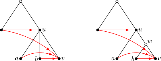
Figure 4: Sliding $b$ into $uv$

Lemma 3.4.

If $(T^{\prime},r^{\prime},\operatorname{\ell}^{\prime},\operatorname{c}’)$ is obtained from $(T,r,\operatorname{\ell},\operatorname{c})$ by sliding a vertex into an edge, then any oriented graph derived from $(T,r,\operatorname{\ell},\operatorname{c})$ can be derived from $(T^{\prime},r^{\prime},\operatorname{\ell}^{\prime},\operatorname{c}’)$.

Proof.

Let $G$ be derived from $T$. The statement follows directly from the fact that the function $\operatorname{c}$ is the restriction of $\operatorname{c}’$ to $V(G)$. ∎

The next lemma shows that all derived graphs can be derived from Burling trees with specific properties. This will reduce the technical difficulty of some proofs.

Lemma 3.5.

Every oriented derived graph $G$ can be derived from a Burling tree $(T,r,\operatorname{\ell},\operatorname{c})$ such that:

1. $r$ is not in $V(G)$,

2. every non-leaf vertex in $T$ has exactly two children,

3. no last-born of $T$ is in $V(G)$.

Proof.

We apply a series of transformations on $(T,r,\operatorname{\ell},\operatorname{c})$ until the conclusion is satisfied.

First transformation: If $r\in V(G)$, build a tree $T^{\prime}$ by adding to $T$ a new vertex $r^{\prime}$ adjacent to $r$. Define $\operatorname{\ell}^{\prime}(r^{\prime})=r$ and $\operatorname{\ell}^{\prime}(v)=\operatorname{\ell}(v)$ for all vertices $v$ of $T$. Moreover set $\operatorname{c}^{\prime}(r^{\prime})=\varnothing$, and do not change the choose function on the rest of the vertices. Notice that $r$ is an isolated vertex in $G$, thus $G$ can be derived from $(T^{\prime},r^{\prime},\operatorname{\ell}^{\prime},\operatorname{c}^{\prime})$.

Second transformation: Suppose that $u$ is a non-leaf vertex of $T$ which has only one child. Build a tree $T^{\prime}$ by adding a new child $v$ to $u$ and define $\operatorname{c}^{\prime}(v)=\varnothing$. Notice that $v$ is a leaf, so it does not have a last-born in $T^{\prime}$. The graph $G$ is also derived from $T^{\prime}$. Apply this process until that every non-leaf vertex in $G$ has at least two children.

Third transformation: Suppose that $u$ is a vertex in $T$ with at least three children, let $v$ be the last-born of $u$ and $a,b$ be two distinct children of $u$ other than $v$. We define a Burling tree $T^{\prime}$ by sliding $b$ into the edge $uv$, and observe that the degree of $u$ in $T^{\prime}$ is smaller than in $T$. And by Lemma 3.4, $G$ can be derived from $T^{\prime}$. We apply the transformation until all vertices have at most two children.

Notice that during this process we decrease the number of children of $u$, the new vertex $w$ has two children, and we do not increase the number of children of any other vertex. Hence the process terminates if we apply the transformation until conclusion (ii) of the lemma is satisfied.

Moreover, notice that in applying the third transformation on a vertex $u$, we do not decrease the number of children of any vertex other than $u$, and once again the new vertex that we create has two children. Thus, after the third transformation, we do not undo the effect of the second transformation.

Notice that after the second and the third transformations, Property (i) of the lemma remains satisfied.

Fourth transformation: If $v$ is a last-born of $T$ that is in $V(G)$, then let $u$ be the parent of $v$. Observe that $\operatorname{c}(v)=\varnothing$. We build a tree $T^{\prime}$ by removing the edge $uv$, adding a new vertex $w$ adjacent to $u$ and $v$, and a new vertex $x$ adjacent to $w$. Define $\operatorname{\ell}^{\prime}(u)=w$, $\operatorname{\ell}^{\prime}(w)=x$ and $\operatorname{\ell}^{\prime}(y)=\operatorname{\ell}(y)$ for all non-leaf vertices $y$ of $T\setminus u$. Define $\operatorname{c}^{\prime}(y)=\operatorname{c}(y)\cup\{w\}$ for every vertex $y\in V(T)$ such that $v\in\operatorname{c}(y)$ and $\operatorname{c}^{\prime}(y)=\operatorname{c}(y)$ otherwise. We see that $G$ can be derived from $(T^{\prime},r^{\prime},\operatorname{\ell}^{\prime},c^{\prime})$, and $v$ is not a last-born in $T^{\prime}$, so we have reduced the number of last-borns of the Burling tree in $V(G)$. Apply this transformation until there is no last-born of the Burling tree in $V(G)$. See Figure 5.

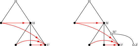
Figure 5: Turning $v$ into a non-last-born

Finally, notice that this transformation does not cancel the effect of the previous ones. This completes the proof of the lemma. ∎

4 Equality of Burling graphs and derived graphs

In this section, we recall the classical definition of the Burling sequence and prove that derived graphs and Burling graphs form the same class.

Burling graphs

There are different equivalent approaches to define Burling graphs. See [2] for the first definition by Burling, or [7] for a second definition. The definition that we use here is the one from [3] (see Appendix B of [3]).

Definition 4.1.

Let $(G,\mathcal{S})$ be a pair where $G$ is a graph and $\mathcal{S}$ is a set of stables sets of $G$. We define a function $\operatorname{\textsc{next-b}}$ associating to a pair $(G,\mathcal{S})$ another pair $(G^{\prime},\mathcal{S}^{\prime})$ as follows:

1. Take a copy of $G$.

2. For each stable set $S\in\mathcal{S}$, take a new copy of $G$ and denote it by $G_{\mathcal{S}}$. Note that the same set of stable sets as $\mathcal{S}$ exists in $G_{\mathcal{S}}$. Denote it by $\mathcal{S}_{S}$.

3. For each $S\in\mathcal{S}$ and $Q\in\mathcal{S}_{S}$, add a new vertex $v_{S,Q}$ adjacent to all vertices in $Q$.

4. Denote by $G^{\prime}$ the obtained graph

5. Consider every stable set of the form $S\cup Q$ and $S\cup\{v_{S,Q}\}$ where $S\in\mathcal{S}$ and $Q\in\mathcal{S}_{S}$. Call $\mathcal{S}^{\prime}$ the set of all these stable sets.

The pair $(G^{\prime},\mathcal{S}^{\prime})$ is defined to be $\operatorname{\textsc{next-b}}(G,\mathcal{S})$.

Starting with $(G_{1},S_{1})$ where $G_{1}=K_{1}$ and $\mathcal{S}_{1}=\{V(G_{1})\}$ and applying the function $\operatorname{\textsc{next-b}}$ iteratively, we define a sequence $(G_{k})_{k\geq 1}$ in which $(G_{k+1},\mathcal{S}_{k+1})=\operatorname{\textsc{next-b}}(G_{k},\mathcal{S}_{k})$. This sequence is called the Burling sequence. In Figure 6, the first three graphs in this sequence are represented. The edges of the graphs are represented in red and the stable sets are represented by dashed curves.

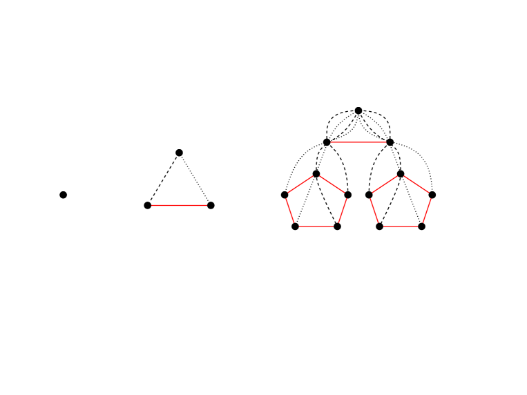
Figure 6: The first three graphs in the Burling sequence

Notice that a copy of the first graph $G_{1}$, which is a single vertex, is present in all the graphs of the sequence, and it is an isolated vertex of them.

The class of Burling graphs is the class consisting of all graphs in the Burling sequence and their induced subgraphs.

Burling proved that the graphs of the Burling sequence have unbounded chromatic number. (See Theorem 1 of [7].) For the sake of completeness, we include the sketch of the proof here. Here, a coloring of a graph is a function that assigns to each vertex a color, in such a way that adjacent vertices receive different colors. By induction, we prove the following statement:

In every coloring of the vertices of $G_{k}$, one of the stable sets in the family $\mathcal{S}_{k}$ receives at least $k$ colors.

This is obvious for $k=1$. Suppose the statement holds for some fixed $k$. Consider a coloring of $G_{k+1}$. By the induction hypothesis, in the first copy of $G_{k}$ in $G_{k+1}$, there exists a stable set $S\in\mathcal{S}_{k}$ which receives at least $k$ colors. Again, by the induction hypothesis, in $G_{S}$, the copy of $G_{k}$ associated to $S$, there exists a stable set $Q\in\mathcal{S}_{S}$ receiving $k$ colors. Now either the $k$ colors of $S$ are the same as the $k$ colors of $Q$, in which case $v_{S,Q}$ has a new color, and therefore $S\cup\{v_{S,Q}\}\in\mathcal{S}_{k+1}$ receives $k+1$ different colors, or the colors in $S$ and $Q$ are different, in which case $S\cup Q\in\mathcal{S}_{k+1}$ receives $k+1$ different colors. This completes the proof.

Tree sequence

Recall that a principal branch of a Burling tree $(T,r,\operatorname{\ell},\operatorname{c})$ is any branch starting in its root $r$ and ending in one of its leaves. The principal set of $(T,r,\operatorname{\ell},\operatorname{c})$ is the set of all vertex-sets of the principal branches of $T$. We denote the principal set of $T$ by $\mathcal{P}(T)$. Notice that there is a one-to-one correspondence between $\mathcal{P}(T)$ and $L(T)$, the set of leaves of $T$.

If a graph $G$ is derived from a Burling tree $T$, then the restriction of each principal branch of $T$ to the vertices of $G$, forms a stable set in $G$. In particular, $\mathcal{P}(T)$, restricted to $V(G)$, is a set of stable sets of $G$.

In this section, we define a sequence $(T_{k})_{k\geq 1}$ of Burling trees and we prove that the sequence $(T_{k},\mathcal{P}_{k})_{k\geq 1}$ of Burling trees and their principle sets is in correspondence to the sequence $(G_{k},\mathcal{S}_{k})_{k\geq 1}$ of Burling graphs. More precisely, we will show that the $k$-th Burling graph $G_{k}$ is isomorphic to the graph fully derived from $T_{k}$, and $S_{k}$ is the same as $\mathcal{P}_{k}=\mathcal{P}(T_{k})$.

To define the mentioned sequence, we first define a function $\operatorname{\textsc{next-t}}$ on Burling trees.

Definition 4.2.

Let $(T,r,\operatorname{\ell},\operatorname{c})$ be a Burling tree, and let $\mathcal{S}$ denote its principal set. We build a Burling structure $(T^{\prime},r^{\prime},\operatorname{\ell}^{\prime},\operatorname{c}^{\prime})$ with principal set $\mathcal{S}^{\prime}$ as follows:

1. Take a copy of $(T,r,\operatorname{\ell},\operatorname{c})$.

2. For each principal branch $P\in\mathcal{S}$ ending in the leaf $l$, pend a leaf $l_{P}$ to $l$, and define $\operatorname{\ell}(l)=l_{P}$. Then put a copy $(T,r,\operatorname{\ell},\operatorname{c})_{P}$ on $l_{P}$, identifying its root with $l_{P}$. Denote the principal set of $(T,r,\operatorname{\ell},\operatorname{c})_{P}$ by $\mathcal{S}_{P}$.

3. For each copy $(T,r,\operatorname{\ell},\operatorname{c})_{P}$, corresponding to a leaf $l\in P$, for each $Q\in\mathcal{S}_{P}$, add a new leaf $l_{P,Q}$ to $l$.

4. to obtain $c^{\prime}$, first extend the function $\operatorname{c}$ naturally to the copies of $(T,r,\operatorname{\ell},\operatorname{c})$, and then also define $\operatorname{c}^{\prime}(l_{P,Q})=Q$ for $P\in\mathcal{S}$ and $Q\in\mathcal{S}_{P}$.

5. Notice that the result is a Burling tree $(T^{\prime},r^{\prime},\operatorname{\ell}^{\prime},\operatorname{c}^{\prime})$.

6. Observe that the principal branches of $T^{\prime}$ are of the form $P\cup Q$ or $P\cup\{l_{P,Q}\}$ for $P\in\mathcal{S}$ and $Q\in\mathcal{S}_{P}$. Thus $\mathcal{S}^{\prime}=\{P\cup Q,P\cup\{l_{P,Q}\}:P\in\mathcal{S},Q\in\mathcal{S}_{P}\}$.

We denote $(T^{\prime},r^{\prime},\operatorname{\ell}^{\prime},\operatorname{c}^{\prime})$ by $\operatorname{\textsc{next-t}}(T,r,\operatorname{\ell},\operatorname{c})$. By abuse of notation, we may write $T^{\prime}=\operatorname{\textsc{next-t}}(T)$.

Starting from $T_{1}$, the one vertex Burling tree, and applying the $\operatorname{\textsc{next-t}}$ function iteratively, we reach a sequence $(T_{k},r_{k},\operatorname{\ell}_{k},\operatorname{c}_{k})_{k\geq 1}$ of Burling trees that we call the tree sequence.

In the rest of this section whenever we use the notation $(G_{k},\mathcal{S}_{k})$, we mean the $k$-th graph in the Burling sequence and its set of stable sets. Similarly, when we write $(T_{k},r_{k},\operatorname{\ell}_{k},\operatorname{c}_{k})$, or by abuse of notation $T_{k}$, we mean the $k$-th Burling tree in the tree sequence.

The next two lemmas are about some properties of the sequence $(T_{k})_{k\geq 1}$.

Lemma 4.3.

Let $v$ be a vertex in $T_{k}$. If $v$ is not a leaf, then it has at least two children in $T_{k}$.

Proof.

We prove the lemma by induction on $k$. For $k=1$, there is nothing to prove. Suppose that the statements are true for $T_{k}$ where $k\geq 1$.

Let $v$ be a vertex in $T_{k+1}=\operatorname{\textsc{next-t}}(T_{k})$ which is not a leaf. The vertex $v$ appears in one of the copies of $T_{k}$, and because it is not a leaf, either it is a non-leaf vertex of a copy of $T_{k}$, and thus it has at least 2 children by the induction hypothesis, or it is a leaf of the main copy of $T_{k}$ in $T_{k+1}$. But notice that as a leaf of the main copy of $T_{k}$, in Step (ii) of Definition 4.2, it receives a child, and in Step (iii) it receives at least one more child. So $v$ has at least 2 children in $T_{k+1}$. ∎

Lemma 4.4.

If $v$ is a non-last-born vertex in $T_{k}$ which is not the root, then $c_{k}(v)\neq\varnothing$. In particular, the last-born brother of $v$ is in $c_{k}(v)$.

Proof.

We prove the lemma by induction on $k$. For $k=1$, there is nothing to prove. Suppose that the statements are true for $T_{k}$ where $k\geq 1$, and suppose that $v$ is a non-last-born vertex in $T_{k+1}$ other than its root. There are two possibilities:

First, $v$ is a non-last-born vertex in one of the copies of $T_{k}$ (either the main copy, or a copy corresponding to a principal branch). In this case, the result follows from the induction hypothesis.

Second, $v$ is a vertex of the form $l_{P,Q}$ as in Step (iii) of Definition 4.2. Then in Step (iv) we define $c_{k+1}(v)$ to be $Q$ which is not empty. ∎

Equality of Burling graphs and derived graphs

We are now ready to prove the equality of Burling graphs and derived graphs.

Lemma 4.5.

For every $k\geq 1$, $G_{k}$ is fully derived from $T_{k}$, and $\mathcal{S}_{k}$ is $\mathcal{P}_{k}=\mathcal{P}(T_{k})$.

Proof.

We prove the lemma by induction on $k$. If $k=1$, the statement holds. Suppose that $G_{k}$ is fully derived from $T_{k}$ and $\mathcal{S}_{k}$ is equal to $\mathcal{P}_{k}$.

To build $T_{k+1}$, to every leaf $l$ of $T_{k}$, we add a new leaf and we pend a copy of $T_{k}$ to this new leaf. Since every leaf in $T_{k}$ identifies exactly one of the principal branches, or by the induction hypothesis, one stable set in $\mathcal{S}_{k}$, this step is equivalent to step (ii) in Definition 4.1. Then for each copy $(T_{k})_{P}$ of $T_{k}$, we add $|\mathcal{P}_{k}|=|\mathcal{S}_{k}|$ new leaves to the leaf corresponding of the principal branch $P$. For a new vertex $l_{P,Q}$ corresponding to the branch $Q\in\mathcal{P}(T_{k})_{P}$, we define the choose-function to be $Q\in(T_{k})_{P}$ which assures that in the graph fully derived from $T$, this vertex is complete to $Q$. Thus these new vertices $l_{P,Q}$ are the vertices $v_{P,Q}$ that we add in step (iii) of Definition 4.1, and $G_{k+1}$ is the graph fully derived from $T_{k+1}$.

Finally, we notice that the vertex sets of the principal branches of $T_{k+1}$ are exactly sets of the form $P\cup Q$ and $P\cup\{l_{P,Q}\}$ for $P\in\mathcal{\mathcal{missing}}P_{k}=\mathcal{S}_{k}$ and $Q\in(\mathcal{P}_{k})_{P}=(\mathcal{S}_{k})_{P}$. Thus $\mathcal{S}_{k+1}=\mathcal{P}_{k+1}$. ∎

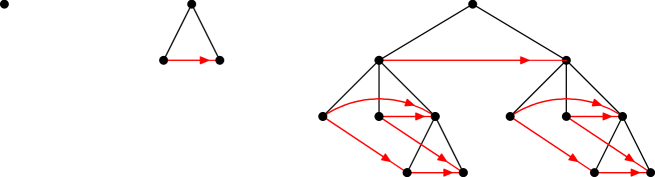
Figure 7: The first three graphs of the Burling sequence seen as fully derived graphs

Figure 7 shows some orientations of the first three graphs of the Burling sequence as fully derived graphs.

Now we define the notion of extension for Burling trees, which is, as we will see formally in Lemma 4.7, closely related to the notion of induced subgraph in fully derived graphs.

Definition 4.6.

Let $(T,r,\operatorname{\ell},\operatorname{c})$ and $(T^{\prime},r^{\prime},\operatorname{\ell}^{\prime},\operatorname{c}^{\prime})$ be two Burling trees. We say that $T^{\prime}$ is an extension of $T$ if there exists an injection $\varphi$ from $V(T)$ to $V(T^{\prime})$ with the following properties:

1. $\varphi(r)=r^{\prime}$,

2. $\varphi$ preserves ancestors, i.e. if $u$ is an ancestor of $v$ in $T$, then $\varphi(u)$ is an ancestor of $\varphi(v)$ in $T^{\prime}$,

3. $\varphi$ preserves the last-born vertices, i.e. if $v\in V(T)$ is a last-born in $T$, then $\varphi(v)$ is a last-born in $T^{\prime}$.

4. $\varphi$ preserves the choose-path function on $T$, i.e. for every vertex $v\in T$, $\varphi(\operatorname{c}(v))=\operatorname{c}^{\prime}(\varphi(v))\cap\varphi(V(T))$.

Lemma 4.7.

Let $G$ and $G^{\prime}$ be two oriented graphs fully derived from $T$ and $T^{\prime}$ respectively. If $T^{\prime}$ is an extension of $T$, then $G$ is an induced subgraph of $G$.

Proof.

Let $\varphi$ be the injection from $V(T)$ to $V(T^{\prime})$. Since $G$ and $G^{\prime}$ are fully derived from $T$ and $T^{\prime}$, $V(G)=V(T)$ and $V(G^{\prime})=V(T^{\prime})$. Thus $\varphi$ can be seen as an injection from $V(G)$ to $V(G^{\prime})$. By property (iv) in Definition 4.6, $v\in\operatorname{c}(u)$ if and only if $\varphi(v)\in\operatorname{c}^{\prime}(\varphi(u))$. In other words, $uv\in A(G)$ if and only if $\varphi(u)\varphi(v)\in A(G^{\prime})$. Thus $G$ is an induced subgraph of $G^{\prime}$. ∎

Next lemma shows that the tree sequence $(T_{k})_{k\geq 1}$ contains all the Burling trees in the extension sense.

Lemma 4.8.

If $(T,r,\operatorname{\ell},\operatorname{c})$ is a Burling tree such that every non-leaf vertex has exactly two children, then there is an integer $i\geq 1$ such that $T_{i}$ is an extension of $T$.

Proof.

We prove the lemma by induction on the number of vertices of $T$.

For the induction step, the smallest possible $T$ is a tree on three vertices: the root $r$, the last-born of the root $v$, and the other child of the root $u$. If $\operatorname{c}(u)=\{v\}$, then $T_{2}$ is an extension of $T$. If $\operatorname{c}(u)=\varnothing$, then $T_{3}$ is an extension of $T$ as shown in Figure 8.

Figure 8: When $\operatorname{c}(u)=\varnothing$, $T_{3}$ (right) is an extension of $T$ (left)

Suppose that the lemma is true for every Burling tree on at most $n$ vertices. Suppose that $T$ on $n>1$ vertices is given.

Consider the set of all the vertices of $T$ which have the maximum distance to $r$. Because every non-leaf vertex in $T$ has two children, there is a non-last-born vertex $x$ in this set. Notice that $x$ has no children. Denote by $p$ the parent of $x$ and by $y$ the last-born of $p$. Notice that $y$ also has the maximum distance to the root, and thus both $x$ and $y$ are leaves of $T$.

Consider the tree $(T^{\prime},r,\operatorname{\ell}^{\prime},\operatorname{c}^{\prime})$, obtained from $T$ by removing the two leaves $x$ and $y$, and restricting the functions $\operatorname{\ell}$ and $\operatorname{c}$. By induction hypothesis, there exist $k$ such that $T_{k}$ is an extension of $T$. Let $\varphi$ be the injection from $V(T)$ to $V(T_{k})$. In the rest of the proof, we will define $\varphi$ on $x$ and $y$ in order to extend $\varphi$ to $V(T)$, in a way that all the four properties of Definition 4.6 remain satisfied.

Now there are two possible cases.

Case 1: $y\in\operatorname{c}(x)$.

If $\varphi(p)$ is not a leaf of $T_{k}$, then define $\varphi(x)$ to be a non-last-born child of $\varphi(p)$, which exists by lemma 4.3, and define $\varphi(y)$ to be the last-born of $\varphi(p)$. By Lemma 4.4, $\varphi(y)$ is in $c_{k}(\varphi(x))$. Notice that this extension of $\phi$ has all the properties of Definition 4.6. Properties (i) to (iii) are easy to verify, and for Property (iv), notice that no descendant of $\varphi(y)$ is in the image of $\varphi$, thus $\varphi(\operatorname{c}(x))=\varphi(\{y\})=\{\operatorname{\ell}_{k}(p)\}=c_{k}(\varphi(y))\cap\operatorname{im}(\varphi)$.

If $\varphi(p)$ is a leaf of $T_{k}$, then consider $T_{k+1}$. In building $T_{k+1}$, every leaf of the first copy of $T_{k}$, including $\varphi(p)$, will receive a last-born and at least one non-last-born child. Define again $\varphi(x)$ to be a non-last-born child of $\varphi(p)$ and $\varphi(y)$ to be the last-born of $\varphi(p)$. See Figure 9. Notice that again $\varphi$ has all the required properties. So $T_{k+1}$ is an extension of $T$.

Figure 9: Case 1 of the proof of Lemma 4.8

Case 2: $y\notin\operatorname{c}(x)$.

If $\varphi(p)$ is not a leaf of $T_{k}$, by 4.3 it has at least two children. Choose two paths starting at two different children of $\varphi(p)$ and ending at two different leafs $l$ and $\operatorname{\ell}^{\prime}$ of $T_{k}$. In $T_{k+1}$, consider $l$ and $\operatorname{\ell}^{\prime}$ in the first copy of $T_{k}$. Define $\varphi(x)$ to be some non-last-born of $l$ in $T_{k+1}$ and $\varphi(y)$ to be the last-born of $\operatorname{\ell}^{\prime}$ in $T_{k+1}$. See Figure 10, left. Notice that $l\neq\operatorname{\ell}^{\prime}$, thus $\varphi(y)\notin\varphi(x)$. The new function $\varphi$ has all the required properties. Hence $T_{k+1}$ is an extension of $T$.

If $\varphi(p)$ is a leaf of $T_{k}$, then consider $T_{k+1}$. In $T_{k+1}$, the vertex $\varphi(p)$ in the main copy of $T_{k}$ has a last-born $l$ and at least one non-last-born. Choose any non-last-born child of $\varphi(p)$ and denote it by $n$. Notice that $n$ is a leaf of $T_{k+1}$. Thus in $T_{k+2}$, this vertex will have a some children, including at least one non-last-born, that we denote by $l^{\prime}$. Notice that $l\notin c_{k+2}(l^{\prime})$. Define $\varphi(x)=l^{\prime}$ and $\varphi(y)=l$. See Figure 10, right. It is easy to check that $\varphi$ has all the properties of Definition 4.6, so $T_{k+2}$ is an extension of $T$.

Figure 10: Case 2 of the proof of Lemma 4.8

∎

Now we can prove the main theorem of the section.

Theorem 4.9.

The class of derived graphs is the same as the class of Burling graphs.

Proof.

Suppose that $H$ is a Burling graph. So $H$ is an induced subgraph of some $G_{k}$ which is a fully derived graph by Lemma 4.5. Thus $H$ is a derived graph.

Now suppose that $H$ is derived from a tree $T$. By Lemma 3.5, we may assume that every non-leaf vertex in $T$ has exactly two children. Notice that $H$ is an induced subgraph of $G$, the graph fully derived from $T$. By Lemma 4.8, there exists $k$ such that $T_{k}$ is an extension of $T$. Moreover, by Lemma 4.5, $G_{k}$ is the graph fully derived from $T_{k}$. Thus by Lemma 4.7, $G$ is an induced subgraph of $G_{k}$, and thus it is a Burling graph. Therefore, so is $H$. ∎

Theorem 4.9 enables us to interchangeably use the words Burling graphs or derived graphs for referring to this class. The advantage of derived graphs to the classical definition of Burling graphs is that thanks to the tree structure, we can study the behavior of the stable sets much better. The Burling tree captures in an easier way both the structure of the stable sets, and the adjacency of vertices in Burling graphs. Moreover, as we will show in the second part of this work, the orientation gives us more information about the properties of this class of graphs.

5 Abstract Burling graphs

In this section, we prove that Burling graphs can be defined as abstract Burling graph, that are graphs arising from two relations defined on a set and satisfying a small number of axioms.

Definition 5.1.

A Burling set is a triple $(S,\operatorname{\prec},\operatorname{\curvearrowright})$ where $S$ is a non-empty finite set, $\operatorname{\prec}$ is a strict partial order on $S$, $\operatorname{\curvearrowright}$ is a binary relation on $S$ that does not have directed cycles, and such that the following axioms hold:

1. if $x\operatorname{\prec}y$ and $x\operatorname{\prec}z$, then either $y\operatorname{\prec}z$ or $z\operatorname{\prec}y$,

2. if $x\operatorname{\curvearrowright}y$ and $x\operatorname{\curvearrowright}z$, then either $y\operatorname{\prec}z$ or $z\operatorname{\prec}y$,

3. if $x\operatorname{\curvearrowright}y$ and $x\operatorname{\prec}z$, then $y\operatorname{\prec}z$,

4. if $x\operatorname{\curvearrowright}y$ and $y\operatorname{\prec}z$, then either $x\operatorname{\curvearrowright}z$ or $x\operatorname{\prec}z$.

Let us give an example of a Burling set. Let $(T,r,\operatorname{\ell},\operatorname{c})$ be a Burling tree, and set $V=V(T)$. For $x,y\in V$, we define $x\operatorname{\prec}y$ if and only if $x$ is a proper descendant of $y$ in $T$ and $x\operatorname{\curvearrowright}y$ if and only if $y\in\operatorname{c}(x)$. Note that $x\operatorname{\curvearrowright}y$ if and only if there is an arc from $x$ to $y$ in the oriented graph fully derived from $(T,r,\operatorname{\ell},\operatorname{c})$.

We show that $(V,\operatorname{\prec},\operatorname{\curvearrowright})$ forms a Burling set. First notice that the proper descendant relation on a rooted tree forms a strict partial order. Second, remember that by Lemma 3.2, the relation $\operatorname{\curvearrowright}$ has no directed cycles. Now we check the four axioms of Definition 5.1. Let $x$, $y$, and $z$ be three elements of $V$:

Axiom (i): Suppose that $x\operatorname{\prec}y$ and $x\operatorname{\prec}z$. So both $y$ and $z$ are ancestors of $x$ in $T$, so they are on the same branch and hence comparable with respect to $\operatorname{\prec}$.

Axiom (ii): Suppose that $x\operatorname{\curvearrowright}y$ and $x\operatorname{\curvearrowright}z$. So $y,z\in\operatorname{c}(x)$. Thus by definition, they are on the same branch and are comparable with respect to $\operatorname{\prec}$.

Axiom (iii): Suppose that $x\operatorname{\curvearrowright}y$ and $x\operatorname{\prec}z$. So $y\in\operatorname{c}(x)$ and thus $y$ is a descendant of $p(x)$. On the other hand, $z$ is an ancestor of $x$, so it is an ancestor of $y$ too, and it is different from $y$. Hence $y\operatorname{\prec}z$.

Axiom (iv): Suppose that $x\operatorname{\curvearrowright}y$ and $y\operatorname{\prec}z$. Let $l$ be the last-born of $p(x)$. So $y$ is a descendant of $l$, and $z$ is an ancestor of $y$. Either $z$ is a descendant of $l$ too, in which case $x\operatorname{\curvearrowright}z$ or $z$ is a proper ancestor of $l$, in which case it is a proper ancestor of $x$ too, i.e. $x\operatorname{\prec}z$.

Lemma 5.2.

Let $S$ be a Burling set, and let $x,y\in S$. At most one of the following holds: $x\operatorname{\curvearrowright}y$, $y\operatorname{\curvearrowright}x$, $x\operatorname{\prec}y$, or $y\operatorname{\prec}x$. In particular, $\operatorname{\curvearrowright}\cap\operatorname{\prec}=\varnothing$.

Proof.

Notice that if any of the four relations hold, then $x\neq y$, because $\operatorname{\prec}$ is a strict partial order and $\operatorname{\curvearrowright}$ has no directed cycle of length 1.

First suppose that $x\operatorname{\curvearrowright}y$. Because $\operatorname{\curvearrowright}$ has no directed cycles, we cannot have $y\operatorname{\curvearrowright}x$. Moreover, if $x\operatorname{\prec}y$, then by Axiom (iii) of Definition 5.1 we must have $y\operatorname{\prec}y$ which is a contradiction. If $y\operatorname{\prec}x$, then by Axiom (iv), we have either $x\operatorname{\curvearrowright}x$ or $x\operatorname{\prec}x$, in both cases, it is a contradiction.

It just remains to check that $x\operatorname{\prec}y$ and $y\operatorname{\prec}x$ cannot happen simultaneously, which is clear by the definition of strict partial orders. ∎

Lemma 5.3.

Let $\operatorname{R}=\operatorname{\curvearrowright}\cup\operatorname{\prec}$. The relation $\operatorname{R}$ has no directed cycle. In particular, $\operatorname{R}$ has some minimal element which is therefore minimal for both $\operatorname{\curvearrowright}$ and $\operatorname{\prec}$.

Proof.

Suppose for the sake of contradiction that there is a cycle in $\operatorname{R}$, and let $x_{1},x_{2},\dots,x_{n}$ be a minimal cycle.

By definition, $n\neq 1$, and by Lemma 5.2, $n\neq 2$.

Now suppose that $n\geq 4$. Notice that none of $\operatorname{\curvearrowright}$ and $\operatorname{\prec}$ has a directed cycle, thus there exists $1\leq i\leq n$, such that $x_{i}\operatorname{\curvearrowright}x_{i+1}$ and $x_{i+1}\operatorname{\prec}x_{i+2}$ (summations modulo $n$). Hence by Axiom (iv), we must have either $x_{i}\operatorname{\curvearrowright}x_{i+2}$ or $x_{i}\operatorname{\prec}x_{i+2}$. In any case, $x_{i}\operatorname{R}x_{i+2}$, which is in contradiction to the minimality of the chosen directed cycle.

Finally, suppose that $n=3$. Up to symmetry, we have $x_{1}\operatorname{\curvearrowright}x_{2}$ and $x_{2}\operatorname{\prec}x_{3}$, and therefore by Axiom (iv), $x_{1}\operatorname{R}x_{3}$. But because this is a cycle, we must have $x_{3}\operatorname{R}x_{1}$. This is in contradiction to Lemma 5.2.

So $\operatorname{R}$ has no directed cycle. So there exists a minimal element in $\operatorname{R}$ which is, by definition, a minimal element for both $\operatorname{\curvearrowright}$ and $\operatorname{\prec}$. ∎

We recall that in a given Burling set $S$, and for an element $s$ in $S$, $[s{\operatorname{\curvearrowright}}]=\{t\in S:s\operatorname{\curvearrowright}t\}$, and $[s{\operatorname{\prec}}]=\{t\in S:s\operatorname{\prec}t\}$.

Lemma 5.4.

Let $s$ be an element of a Burling set $S$. Then there exists an ordering of the elements of $[s{\operatorname{\curvearrowright}}]$ such as $u_{1},u_{2},\dotsm u_{k}$ and an ordering of the elements of $[s{\operatorname{\prec}}]$ such as $v_{1},v_{2},\dots v_{l}$ such that $u_{1}\operatorname{\prec}u_{2}\operatorname{\prec}\dots\operatorname{\prec}u_{k}\operatorname{\prec}v_{1}\operatorname{\prec}v_{2}\operatorname{\prec}\dots\operatorname{\prec}v_{l}$.

Proof.

By Axiom (ii) of Burling sets, all the elements of $[s{\operatorname{\curvearrowright}}]$ form a chain $u_{1}\operatorname{\prec}u_{2}\operatorname{\prec}\dots\operatorname{\prec}u_{k}$. Moreover, by Axiom (i), all the elements of $[s{\operatorname{\prec}}]$ also form a chain $v_{1}\operatorname{\prec}v_{2}\operatorname{\prec}\dots\operatorname{\prec}v_{l}$. Finally, $u_{k}\operatorname{\prec}v_{1}$ follows from Axiom (iii) since $s\operatorname{\curvearrowright}u_{k}$ and $s\operatorname{\prec}v_{1}$. ∎

Let $(S,\operatorname{\prec},\operatorname{\curvearrowright})$ be a Burling set. We define the oriented graph $G$ derived from $(S,\operatorname{\prec},\operatorname{\curvearrowright})$ as the oriented graph on vertex-set $S$ such that for $x,y\in S$, $xy\in A(G)$ if and only if $x\operatorname{\curvearrowright}y$. We denote $G$ by $\operatorname{\Gamma}(S)$, and we say that $G$ is an abstract Burling graph.

Notice that if $S$ is a Burling set and $G=\operatorname{\Gamma}(S)$, then for every induced subgraph $G^{\prime}$ of $G$, $S^{\prime}=V(G^{\prime})$ as a subset of $S$ is itself a Burling set with inherited relations $\operatorname{\prec}$ and $\operatorname{\curvearrowright}$, and moreover $G^{\prime}=\operatorname{\Gamma}(S^{\prime})$.

Equality of abstract Burling graphs and Burling graphs

Lemma 5.5.

Every oriented derived graph is an abstract Burling graph.

Proof.

We checked after Definition 5.1 that if $T$ is a Burling tree, then $V=V(T)$ forms a Burling set, and from there, it follows easily that the graph fully derived from $T$ is exactly $\operatorname{\Gamma}(V)$. Thus every fully derived Burling graph is an abstract Burling graph. Moreover, since abstract Burling graphs form a hereditary class, every derived graph is an abstract Burling graph. ∎

Lemma 5.6.

Let $G$ be an oriented graph. If $G=\operatorname{\Gamma}(S)$ for some Burling set $S$, then $G$ is an oriented derived graph.

Proof.

We prove the following statement by induction on the number of elements of $S$.

Statement 1.

There exists a Burling tree $(T,r,\operatorname{\ell},\operatorname{c})$ such that $S\subseteq V(T)$, and for every two distinct elements $x$ and $y$ in $S$:

1. $x\operatorname{\prec}y$ if and only if $x$ is a descendant of $y$ in $T$,

2. $x\operatorname{\curvearrowright}y$ if and only if $y\in\operatorname{c}(x)$ in $T$.

If $|S|=1$, then the result obviously holds. Suppose that the statement holds for every Burling set on at most $k-1$ elements, and let $S$ be a Burling set on $k\geq 2$ elements.

Let $v\in S$ be a minimal element of $\operatorname{\curvearrowright}\cup\operatorname{\prec}$ which exists by Lemma 5.3. Set $S^{\prime}=S\setminus\{v\}$. By the induction hypothesis, there exists a Burling tree $(T^{\prime},r^{\prime},\operatorname{\ell}^{\prime},\operatorname{c}^{\prime})$ such that $S^{\prime}\subseteq V(T^{\prime})$ and the two properties of the statement hold.

Now let $[v{\operatorname{\curvearrowright}}]=\{u_{1},u_{2},\dots,u_{m}\}$ and $[v{\operatorname{\prec}}]=\{w_{1},w_{2},\dots,w_{n}\}$ (both possibly empty). By Lemma 5.4, suppose without loss of generality that $u_{1}\operatorname{\prec}u_{2}\operatorname{\prec}\dots\operatorname{\prec}u_{m}\operatorname{\prec}w_{1}\operatorname{\prec}w_{2}\operatorname{\prec}\dots\operatorname{\prec}w_{n}$. Thus by the induction hypothesis, they appear on a same branch of $T^{\prime}$. So from the root to the leaf, they appear in this order: $w_{n},\dotsm w_{1},u_{n},\dots,u_{1}$. Now we consider two cases:

Case 1: $[v{\operatorname{\prec}}]=\varnothing$. In this case, add a parent $r$ to $r^{\prime}$ and define $\operatorname{\ell}(r)=r^{\prime}$. Then add $v$ as a child of $r$. If $[v{\operatorname{\curvearrowright}}]=\varnothing$, then define $\operatorname{c}(v)=\varnothing$. Otherwise, let $P$ be the set of vertices on the path between $r^{\prime}$ and $u_{1}$, including both of them, and define $\operatorname{c}(v)=P$. Call this new Burling tree $T$.

Case 2: $[v{\operatorname{\prec}}]\neq\varnothing$. In this case, if $w_{1}$ is a leaf, and hence $[v{\operatorname{\curvearrowright}}]=\varnothing$, then add $v$ as a last-born child of $w_{1}$ and define $\operatorname{c}(v)=\varnothing$. If $w_{1}$ is not a leaf, then add $v$ as a non-last-born child of $w_{1}$. If $[v{\operatorname{\curvearrowright}}]=\varnothing$, define $\operatorname{c}(v)=\varnothing$. Otherwise, let $P$ be the set of vertices on the path between $\operatorname{\ell}(w_{1})$ and $u_{1}$, and define $\operatorname{c}(v)=P$. Call the obtained Burling tree $T$.

In both cases, we obviously have $S\subseteq V(T)$, so it remains to prove the two properties of the statement. For any two distinct elements of $S$ which are both different from $v$, the result follows from the induction hypothesis. So consider $v$ and an element $u$ of $S$ different from $v$. Notice that by minimality of $v$ with respect to both relations, we have neither $u\operatorname{\curvearrowright}v$ nor $u\operatorname{\prec}v$ in $S$, and by the construction of $T$, in both cases, $v$ is not in $\operatorname{c}(u)$, and it has no descendant, so in particular, $u$ is not a descendant of $v$. Moreover, by construction of $T$ in both cases, if $v\operatorname{\prec}u$ in $S$, then $v$ is a descendant of $u$ in $T$, and if $v\operatorname{\curvearrowright}u$ in $S$, then $u\in\operatorname{c}(v)$ in $T$.

Now suppose that $x$ is an element of $S$, and in $T$, $x$ is an ancestor of $v$, and thus we are necessarily in case 2. We prove that $v\operatorname{\prec}x$. If $x=w_{1}$, then the result is immediate. Otherwise, $x$ is an ancestor of $w_{1}$. Thus by the induction hypothesis, $w_{1}\operatorname{\prec}x$. On the other hand, $v\operatorname{\prec}w$. Since $\operatorname{\prec}$ is a strict partial order, $v\operatorname{\prec}x$.

Finally, suppose that $x$ is an element of $S$ and in $T$, $x\in\operatorname{c}(v)$. We show that $v\operatorname{\curvearrowright}x$ in $S$. From $x\in\operatorname{c}(v)$, we know that $x$ is a vertex among the vertices of the path from the last-born of $w_{1}$ to $u_{1}$. If $x=u_{1}$, then the result is immediate. If not, we have $v\operatorname{\curvearrowright}u_{1}$ and $u_{1}\operatorname{\prec}x$. So by Axiom (i) of Definition 5.1, either $v\operatorname{\curvearrowright}x$ or $v\operatorname{\prec}x$. But the latter is not possible because otherwise from $v\operatorname{\prec}x$ and the fact that $v\neq x$, we know that $x$ is either $w_{1}$ or it is an ancestor of $w_{1}$ in $T$. But this is not possible, because $x\in\operatorname{c}(v)$.

To complete the proof we notice that $G$ is exactly the subgraph of the graph derived from $T$, induced by the vertices of $S$. ∎

Theorem 5.7.

The class of abstract Burling graphs is equal to the class of derived graphs, and therefore to the class of Burling graphs.

Proof.

The proof follows directly from Lemmas 5.5 and 5.6. ∎

We remark here that even though the classes of graphs derived from Burling sets and the graphs derived from Burling trees are the same, there is no immediate one-to-one correspondence between Burling sets and Burling graphs. Burling sets do not need notions equivalent to root and last-born. This is what makes them a general object to work with. On the other hand, derived graphs, having all these specific notions, provide strong tools to deduce structural results, as we will see in the second part of this work.

Topological orderings

We here make several remarks about topological orderings of the vertices in Burling graphs, and BFS and DFS algorithms on them. We do not really need these easy observations (and therefore omit their straightforward formal proofs), but we believe that they help to understand the next section.

It was observed in Lemma 3.2 that oriented derived graphs have no directed cycles. And in Lemma 5.3, we go further and observe that the union of the relations $\operatorname{\prec}$ and $\operatorname{\curvearrowright}$ has no directed cycles (which is easy to see directly on an oriented graph derived from a tree). This means that when an oriented graph $G$ is derived from a tree $T$, if one orients every edge of $T$ from the root to the bottom, then the oriented graph $G^{*}$ on $V(T)=V(G)$ with the union of arcs from $T$ and from $G$ has no directed cycle.

This implies that there should exist a topological ordering of $G^{*}$. And indeed, there is a natural way to find one: with BFS applied to $T$ (starting at the root, and with priority given to non-last-borns). If we denote by $\operatorname{s}(v)$ the opposite of the number given by BFS to each vertex, we have the following: if $u\operatorname{\prec}v$ or $u\operatorname{\curvearrowright}v$, then $\operatorname{s}(u)<\operatorname{s}(v)$. See Figure 11.

Now, in $G^{*}$, change the orientation of every arc of $G$ (but keep the arcs of $T$ from root to leaves). Again, it is easy to check that there is no directed cycle, so there should exist a topological ordering again. This time, an ordering may be obtained with DFS (starting at the root and with priority given to the last-born). If denote by $\operatorname{\overline{s}}(v)$ the opposite of the number given by DFS to each vertex, we have the following: if $v\operatorname{\prec}u$ or $u\operatorname{\curvearrowright}v$, then $\operatorname{\overline{s}}(u)<\operatorname{\overline{s}}(v)$. An example is represented in Figure 11.

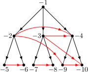
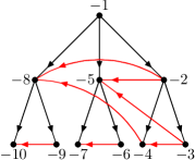
Figure 11: Functions $\operatorname{s}$ and $\operatorname{\overline{s}}$ viewed as topological orderings. Every arc is from a number to a smaller number.

We sum up the main properties of $\operatorname{s}$ and $\operatorname{\overline{s}}$, as defined in this paragraph, in the next lemma. As we will see in the next section, in geometrical interpretations of Burling graphs, there are natural geometrical counterparts of the functions $\operatorname{s}$ and $\operatorname{\overline{s}}$, with each time a similar lemma.

Lemma 5.8.

If $A\operatorname{\prec}B$, then $\operatorname{s}(A)<\operatorname{s}(B)$ and $\operatorname{\overline{s}}(A)<\operatorname{\overline{s}}(B)$. If $A\operatorname{\curvearrowright}B$, then $\operatorname{s}(A)<\operatorname{s}(B)$ and $\operatorname{\overline{s}}(A)>\operatorname{\overline{s}}(B)$.

6 Burling graphs as intersection graphs

In this section, we define three classes of graphs: strict frame graphs, strict line segment graphs, and strict box graphs. We show that they are all equal to the class of Burling graphs.

Strict frame graphs

A frame in $\mathbb{R}^{2}$ is the boundary of an axis-aligned rectangle. Intersection graphs of frames are called frame graphs. Frame graphs clearly form a hereditary class of graphs. The class of restricted frame graphs, defined in [3] (Definition 2.2.), is a subclass of frame graphs. They are the frame graphs with some extra restrictions.

Definition 6.1.

A set of frames in the plane is restricted if it has the following restrictions:

1. there are no three frames, which are mutually intersecting (in other words, the intersection graph of the frames is triangle-free),

2. corners of a frame do not coincide with any point of another frame,

3. the left side of any frame does not intersect any other frame,

4. if the right side of a frame intersects a second frame, this right side intersects both the top and bottom of this second frame,

5. if two frames have non-empty intersection, then no frame is (entirely) contained in the intersection of the regions bounded by the two frames. If frames $A$ and $B$ intersect as in Figure 12, we say that frame $A$ enters frame $B$.

The only possibility for two frames to intersect with these restrictions is shown in Figure 12. In such case, we say that the frame $A$ enters the frame $B$.

Figure 12: Intersection of two frames in restricted frame graphs

Figure 13: A graph obtained from $K_{5}$ by subdividing some edges and its presentation as a restricted frame graph

Figure 14: A necklace and its presentation as a restricted frame graph

Figure 15: A wheel and its presentation as a restricted frame graph. It is easy to see that subdividing the dashed edges yields to restricted frame graphs (see also Appendix A of [3]).

A restricted frame graph is the intersection graph of a restricted set of frames in the plane. An oriented restricted frame graph is a frame graph such that every edge $AB$ is oriented from $A$ to $B$ when frame $A$ enters frame $B$.

See Figures 15, 15 and 15 for some examples of restricted frame graphs. It is worth noting that in the second part of this work, we prove that non of these graphs are Burling graphs.

Now we introduce the class of strict frame graphs, a subclass of restricted frame graphs, and show that it is equal to the class of Burling graphs.

Definition 6.2.

A restricted set of frames in the plane is strict if for any two frames $A$ and $B$ such that $A$ is entirely inside $B$, when a frame $C$ intersects both, $C$ enters both $A$ and $B$. See Figure 16.

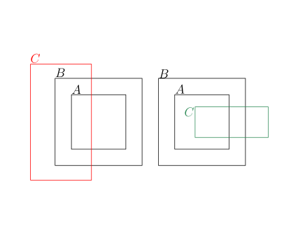
Figure 16: Left: the forbidden structure in strict frame graph, right: the allowed structure

A strict frame graph is the intersection graph of a strict set of frames in the plane. An oriented strict frame graph is a strict frame graph, oriented as an oriented restricted frame graph.

Let $F$ be a non-empty finite strict set of frames in the plane. Define $A\operatorname{\prec}B$ if and only if $A$ is entirely inside $B$. Define $A\operatorname{\curvearrowright}C$ if and only if $A$ enters $C$. We denote by $A\operatorname{{}^{\circ}}$ the area that frame $A$ encloses. Two frames are comparable if $A\operatorname{{}^{\circ}}\cap B\operatorname{{}^{\circ}}\neq\varnothing$ and incomparable otherwise. Note that in a strict set of frames, two frames are comparable if and only if one of them enters the other or is inside the other.

We denote by $\operatorname{s}(A)$ the vertical length of a frame $A$ and by $\operatorname{\overline{s}}(A)$ the maximum real number $x$ such that $x$ is the $x$-coordinate of a point of $A$.

Lemma 6.3.

If $A\operatorname{\prec}B$, then $\operatorname{s}(A)<\operatorname{s}(B)$ and $\operatorname{\overline{s}}(A)<\operatorname{\overline{s}}(B)$. If $A\operatorname{\curvearrowright}B$, then $\operatorname{s}(A)<\operatorname{s}(B)$ and $\operatorname{\overline{s}}(A)>\operatorname{\overline{s}}(B)$.

Proof.

Obvious from the definitions. ∎

Lemma 6.4.

For every non-empty finite and strict set of frames $F$, the triple $(F,\operatorname{\prec},\operatorname{\curvearrowright})$ forms a Burling set.

Proof.

First, $\operatorname{\prec}$ is obviously transitive and asymmetric, so it is a strict partial order. Moreover, by Lemma 6.3, the relation $\operatorname{\curvearrowright}$ cannot have any directed cycle. Now we prove that the four axioms hold. Now we prove that the four axioms of Burling sets hold.

Axiom (i): If $A\operatorname{\prec}B$ and $A\operatorname{\prec}C$, $C\operatorname{{}^{\circ}}$ and $B\operatorname{{}^{\circ}}$ both contain $A$ and thus their intersection is not empty, so $B$ and $C$ are comparable. Now we cannot have $B\operatorname{\curvearrowright}C$ or $C\operatorname{\curvearrowright}B$, because it contradicts item (v) of Definition 6.1. Thus either $B\operatorname{\prec}C$ or $C\operatorname{\prec}B$.

Axiom (ii): If $A\operatorname{\curvearrowright}B$ and $A\operatorname{\curvearrowright}C$, then again $B\operatorname{{}^{\circ}}\cap C\operatorname{{}^{\circ}}\neq\varnothing$, so $B$ and $C$ are comparable. But because $F$ is triangle-free, we cannot have $B\operatorname{\curvearrowright}C$ or $C\operatorname{\curvearrowright}B$. So either $B\operatorname{\prec}C$ or $C\operatorname{\prec}B$.

Axiom (iii): if $A\operatorname{\curvearrowright}B$ and $A\operatorname{\prec}C$, then by Lemma 6.3, $\operatorname{\overline{s}}(B)<\operatorname{\overline{s}}(A)<\operatorname{\overline{s}}(C)$. Since there are points of $A\operatorname{{}^{\circ}}$ which are in both $B\operatorname{{}^{\circ}}$ and $C\operatorname{{}^{\circ}}$, $B$ and $C$ are comparable. Since $\operatorname{\overline{s}}(B)<\operatorname{\overline{s}}(C)$, by Lemma 6.3, we cannot have $B\operatorname{\curvearrowright}C$ or $C\operatorname{\prec}B$. Moreover, $C\operatorname{\curvearrowright}B$ contradicts the restriction of Definition 6.2. Thus $B\operatorname{\prec}C$.

Axiom (iv): If $A\operatorname{\curvearrowright}B$ and $B\operatorname{\prec}C$, then by Lemma 6.3, $\operatorname{s}(A)<\operatorname{s}(B)<\operatorname{s}(C)$. There are points of $A\operatorname{{}^{\circ}}$ which are inside $C\operatorname{{}^{\circ}}$. So $A$ and $C$ are comparable. Since $\operatorname{s}(A)<\operatorname{s}(C)$, by Lemma 6.3, we cannot have $C\operatorname{\curvearrowright}A$ or $C\operatorname{\prec}A$. So, $A\operatorname{\curvearrowright}C$ or $A\operatorname{\prec}C$. ∎

Lemma 6.5.

Every Burling graph is a strict frame graph.

Proof.

If $G$ is a derived graph, then by theorem 4.9 it is an induced subgraph of a graph $G_{k}$ in the Burling sequence. It is easy to check that in the geometrical representation of the Burling sequence in [6] one never creates the forbidden structure of Definition 6.2. One can see the construction of the graphs in the Burling sequence as restricted frame graphs in [6, 3], and check that in their construction, the forbidden constraint of Definition 6.2 does not happen. Moreover, we notice restriction of frames to an induced subgraph, does not create any of the forbidden constraints. ∎

Theorem 6.6.

The class of strict frame graphs is equal to the class of Burling graphs.

Proof.

By Lemma 6.4, every frame graph, is the underlying graph of an abstract Burling graph, and therefore by Theorems 5.7, a Burling graphs. This, along with Lemma 6.5, completes the proof. ∎

Strict line segment graphs

Let $l$ be a non-vertical line segment in $\mathbb{R}^{2}$. We can characterize $l$ by $y=ax+b$ for $x\in[\alpha,\beta]$. The number $a$ is the slope of $l$. We say that $l$ has positive slope if $a$ is a finite positive number (in which case $l$ is neither horizontal nor vertical). We denote the interval $[\alpha,\beta]$ by $\operatorname{X-span}(l)$, and the interval $[a\alpha+b,a\beta+b]$ by $\operatorname{Y-span}(l)$. Finally, for $l$ with positive slope, we define the territory of $l$ to be the unbounded polyhedron defined by $y\geq ax+b$ and $y\in\operatorname{Y-span}(l)$. We denote the territory of $l$ by $\mathcal{T}(l)$. See Figure 17.

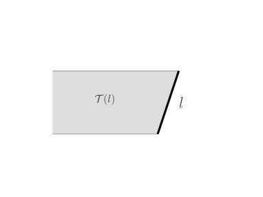
Figure 17: The gray area is the territory of segment $l$.

Definition 6.7.

Let $L$ be a finite set of line segments in $\mathbb{R}^{2}$. We call $L$ a strict set of line segments if the following hold:

1. all the segments in $L$ have positive slopes,

2. no end-point of any line segment lies on another line segment,

3. there exist no three pairwise intersecting line segments in $L$ (in other words, the intersection graph of $L$ is triangle-free),

4. for any two non-intersecting line segments $l$ and $m$, if there exists a point $p$ of $m$ such that $p\in\mathcal{T}(l)$, then $m$ is entirely in $T(l)$ and $\operatorname{Y-span}(m)\subsetneq\operatorname{Y-span}(l)$,

5. if $l$ and $k$ are two intersecting segments, then there are no segments entirely inside $\mathcal{T}(l)\cap\mathcal{T}(k)$,

6. If $k$ and $l$ are two intersecting segments such that the slope of $k$ is less than the slope of $l$, then $\operatorname{Y-span}(k)\subsetneq\operatorname{Y-span}(l)$ and $\operatorname{X-span}(l)\subsetneq\operatorname{X-span}(k)$ such that the maximum of $\operatorname{X-span}(l)$ is strictly less than the maximum of $\operatorname{X-span}(k)$. See Figure 18,

   

   Figure 18: two intersecting segments

7. for any two non-intersecting line segments $l$ and $m$ such that one is in the territory of the other, if a line segment $k$ intersects both of them, then the slope of $k$ is strictly less than both the slope of $l$ and the slop of $m$, as illustrated in Figure 19.

   

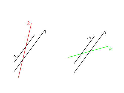
   Figure 19: Left: forbidden and right: allowed structure in constraint (vii).

Let $L$ be a strict finite set of line segments in the plane. Define $l\operatorname{\prec}k$ if and only if $l$ is in the territory of $k$, and define $l\operatorname{\curvearrowright}k$ if and only if $l$ and $k$ have non-empty intersection and the slope of $l$ is less than the slope of $k$.

Note that by Constraint (ii) of Definition 6.7, intersecting line segments must have distinct slopes.

Lemma 6.8.

If for two non-intersecting line segments $l$ and $m$ we have $\mathcal{T}(l)\cap\mathcal{T}(m)\neq\varnothing$, then $\mathcal{T}(l)\subseteq\mathcal{T}(m)$ or $\mathcal{T}(m)\subseteq\mathcal{T}(l)$.

Proof.

Since $\mathcal{T}(l)\cap\mathcal{T}(m)\neq\varnothing$, $\operatorname{Y-span}(l)\cap\operatorname{Y-span}(m)\neq\varnothing$. Thus necessarily one of them has some points inside the territory of the other, and thus by Constraint (iv), is entirely inside the territory of the other. ∎

We denote by $\operatorname{s}(l)$ the length of the interval $\operatorname{Y-span}(l)$ and by $\operatorname{\overline{s}}(l)$ the maximum real number $x$ such that $x$ is the $x$-coordinate of a point of $l$, i.e. the maximum of $\operatorname{X-span}(l)$.

Lemma 6.9.

If $l\operatorname{\prec}k$, then $\operatorname{s}(l)<\operatorname{s}(k)$ and $\operatorname{\overline{s}}(l)<\operatorname{\overline{s}}(k)$. If $l\operatorname{\curvearrowright}k$, then $\operatorname{s}(l)<\operatorname{s}(k)$ and $\operatorname{\overline{s}}(l)>\operatorname{\overline{s}}(k)$.

Proof.

If $l\operatorname{\prec}k$, then $\operatorname{s}(l)<\operatorname{s}(k)$ and $\operatorname{\overline{s}}(l)<\operatorname{\overline{s}}(k)$ because $l$ is in the territory of $k$. The inequalities are strict because of Constraint (iv) of Definition 6.7.

If $l\operatorname{\curvearrowright}k$, then $\operatorname{s}(l)<\operatorname{s}(k)$ and $\operatorname{\overline{s}}(l)>\operatorname{\overline{s}}(k)$ because of Constraint (vi) of Definition 6.7. ∎

Lemma 6.10.

$(L,\operatorname{\prec},\operatorname{\curvearrowright})$ forms a Burling set.

Proof.

First, $\operatorname{\prec}$ is obviously transitive and asymmetric, so it is a strict partial order. Moreover, by Lemma 6.9, the relation $\operatorname{\curvearrowright}$ cannot have any directed cycle. Now we prove that the four axioms of Burling sets hold.

Axiom (i): If $k\operatorname{\prec}l$ and $k\operatorname{\prec}m$, then because of Constraint (v) of Definition 6.7, $l$ and $m$ do not intersect. Moreover, because $k$ is inside the territory of both $l$ and $m$, then by Lemma 6.8, one of them is inside the territory of the other.

Axiom (ii): If $k\operatorname{\curvearrowright}l$ and $k\operatorname{\curvearrowright}m$, then by Constraint (iii), $m$ and $l$ do not intersect. Moreover, notice that by Constraint (vi), the leftmost point of $k$ (the lower endpoint of $k$) is inside the territory of both $l$ and $m$. Thus by Lemma 6.8, one of them is inside the territory of the other.

Axiom (iii): If $k\operatorname{\curvearrowright}l$ and $k\operatorname{\prec}m$, then by Lemma 6.9, $\operatorname{\overline{s}}(l)<\operatorname{\overline{s}}(k)<\operatorname{\overline{s}}(m)$. So, if $l$ and $m$ intersect, then by Lemma 6.9 again, $m\operatorname{\curvearrowright}l$. So, $k$, $l$ and $m$ contradict Constraint (vii). Hence, $l$ and $m$ do not intersect. So, the segment $k$ and thus the intersection of $k$ and $l$ is in the territory of $m$, so by property (iv), $l$ is in the territory of $m$, i.e. $l\operatorname{\prec}m$.

Axiom (iv): If $k\operatorname{\curvearrowright}l$ and $l\operatorname{\prec}m$, then two cases are possible. Case 1: $k$ and $m$ do not intersect. Let $p=(x,y)$ denote the intersection point of $k$ and $l$. Because $p$ is inside the territory of $m$, by Constraint (iv), $k\operatorname{\prec}m$. Case 2: $k$ and $m$ intersect. Then, by Lemma 6.9, $s(k)<s(l)<s(m)$. So $k\operatorname{\curvearrowright}m$.

∎

A strict line segment graph is the intersection graph of a strict set of line segments in the plane.

Lemma 6.11.

Every Burling graph is a strict line segment graph.

Proof.

In [7], graphs of the Burling sequence as presented as line segment graphs. One can check easily that in this construction, all the constraints of Definition 6.7 hold. Now, because every Burling graph is an induced subgraph of a graph in the Burling sequence, and because removing line segments from a strict set of line segments leaves a strict set of line segments, the proof is complete. ∎

Theorem 6.12.

The class of strict line segment graphs is equal to the class of Burling graphs.

Proof.

By Lemma 6.10, every line segment graph, is the underlying graph of an abstract Burling graph, and therefore by Theorems 5.7, a Burling graph. This, along with Lemma 6.11, completes the proof. ∎

Strict box graphs

Let $S$ be a strict set of frames in the $\mathbb{R}^{2}$. Suppose that to each frame $A\in S$ is associated a non-empty interval $I_{A}$ of $\mathbb{R}$. The set of intervals is compatible with $S$ if for all pairs $A,B\in S$ we have:

• if $A$ enters $B$, then $I_{B}\subsetneq I_{A}$ and

• if $A$ is inside $B$ then $I_{A}\cap I_{B}=\varnothing$.

Note that if $A$ and $B$ are incomparable, then there is no condition on $I_{A}$ and $I_{B}$ (in particular, their intersection can be empty or not).

Lemma 6.13.

For every finite strict set $S$ of frames in the plane, there exists a set of intervals compatible with $S$.

Proof.

By lemma 6.4, the intersection graph of $S$ is an abstract Burling graph. Hence by Lemma 5.6, $G$ can be derived from a Burling tree. So, by Lemma 3.5, $G$ is isomorphic to a graph $H$ derived from a Burling tree $(T,r,\operatorname{\ell},\operatorname{c})$ such that $r$ is not in $V(H)$, every non-leaf vertex in $T$ has exactly two children, and no last-born of $T$ is in $V(G)$. So, every frame $A$ of $S$ corresponds to a vertex $v_{A}\neq r$ of $H$ that is not a last-born. Moreover, $A$ is inside $B$ if and only if $v_{A}$ is a descendant of $v_{B}$ in $T$ and $A$ enters $B$ if and only if $v_{B}\in c(v_{A})$.

Hence, it is enough to prove that we may associate to every vertex $v$ of $H$ an interval $I_{z}$ in such a way that for all vertices $u,v$ of $H$:

• if $u\in c(v)$, then $I_{u}\subsetneq I_{v}$ and

• if $u$ is a proper descendant of $v$ then $I_{u}\cap I_{v}=\varnothing$.

We now define the intervals. We first perform a DFS search of $T$, starting at the root and giving priority to the last-borns. This defines an integer $f(v)$ for each vertex $v$ of $T$ satisfying $f(r)=1$, and for every non-leaf vertex $v$ with last-born child $u$ and non-last-born child $w$, $f(u)=f(v)+1$ and

$$f(w)=\max\{f(x):\text{ $x$ is a descendant of $u$}\}+1.$$

See Figure 20.

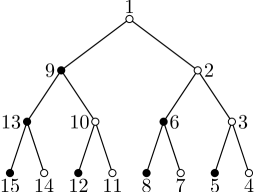
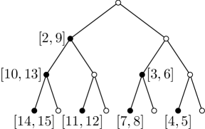
Figure 20: Intervals associated to the non-last-borns of a Burling tree.

Let $w$ be a vertex of $H$. So, $w$ is a vertex of $T$ that is neither $r$ nor a last-born. It follows that $u$ has a parent $v$ that has a last-born child $u$. We associate to $w$ the interval $[f(u),f(w)]$ (note that $f(u)<f(w)$ since we apply DFS with priority to the last-borns).

Suppose that $w$ is a proper descendant of $w^{\prime}$, and their intervals are $[f(u),f(w)]$ and $[f(u^{\prime}),f(w^{\prime})]$ with notation as above. In fact, both $u$ and $w$ are descendant of $w^{\prime}$, so by the properties of DFS, $f(u)>f(w^{\prime})$. This implies that $[f(u),f(w)]$ and $[f(u^{\prime}),f(w^{\prime})]$ are disjoint.

Suppose that $w^{\prime}\in c(w)$, and their intervals are $[f(u),f(w)]$ and $[f(u^{\prime}),f(w^{\prime})]$ with notation as above. Note that $u^{\prime}$ and $w^{\prime}$ are both descendants of $u$. So $f(u)<f(u^{\prime})<f(w^{\prime})$. And since $w^{\prime}$ is a descendant of $u$, $f(w^{\prime})<f(w)$. Hence $[f(u^{\prime}),f(w^{\prime})]\subsetneq[f(u),f(w)]$. ∎

When an interval $I$ is associated to a frame $A$ of $\mathbb{R}^{2}$, there is a natural way to define an axis-align box of $\mathbb{R}^{3}$: $\{(x,y,z):(x,y)\in A\operatorname{{}^{\circ}},z\in I\}$. This is the box associated to $A$ and $I$.

A set of axis-aligned boxes of $\mathbb{R}^{3}$ is strict if it can be obtained from a strict set $S$ of frames by considering of set of intervals compatible with $S$, and by taking for each frame $A$ and each interval $I_{A}$ the box associated to $A$ and $I_{A}$.

Lemma 6.14.

Suppose that a strict set $S^{\prime}$ of boxes is obtained from a strict set of frames $S$. Let $A,B\in S$ be frames, and $A^{\prime},B^{\prime}$ be the respective boxes associated to them. Then $A\cap B\neq\varnothing$ if and only if $A^{\prime}\cap B^{\prime}\neq\varnothing$. In particular, the intersection graph of $S$ is isomorphic to the intersection graph of $S^{\prime}$.

Proof.

If $A$ enters $B$, then $A^{\prime}\cap B^{\prime}\neq\varnothing$ because both the frames and the interval associated to them have a non-empty intersection. If $A$ is inside $B$, then $A^{\prime}\cap B^{\prime}=\varnothing$ because the intervals associated to $A$ and $B$ are disjoint. If $A$ and $B$ are incomparable, then $A^{\prime}\cap B^{\prime}=\varnothing$ because $A\operatorname{{}^{\circ}}\cap B\operatorname{{}^{\circ}}=\varnothing$. ∎

A strict box graph is the intersection graph of a strict set of boxes of $\mathbb{R}^{3}$.

Theorem 6.15.

The class of strict box graphs is equal to the class of Burling graphs.

Proof.

Suppose that $G$ is a Burling graph. Then, by Theorem 6.6, $G$ is the intersection graph of a strict set $S$ of frames. By Lemma 6.13, a set of intervals compatible with $S$ exists. Hence, by Lemma 6.14, $G$ is isomorphic to a strict box graph.

Suppose conversely that $G$ is a strict box graph. Then, by definition, it arises from a strict set of frames and a set of interval compatible with it. Hence, by Lemma 6.14, $G$ is isomorphic to a strict frame graph. So by Theorem 6.6, $G$ is a Burling graph. ∎

References

- [1] John Adrian Bondy and Uppaluri Siva Ramachandra Murty, Graph theory with applications, Elsevier, New York, 1976.
- [2] James Perkins Burling, On coloring problems of families of polytopes (PhD thesis), University of Colorado, Boulder (1965).
- [3] Jérémie Chalopin, Louis Esperet, Zhentao Li, and Patrice Ossona de Mendez, Restricted frame graphs and a conjecture of Scott, Electron. J. Comb. 23 (2016), no. 1, P1.30.
- [4] James Davies, Triangle-free graphs with large chromatic number and no induced wheel, arXiv:2104.05907, 2021.
- [5] Tomasz Krawczyk, Arkadiusz Pawlik, and Bartosz Walczak. Coloring triangle-free rectangle overlap graphs with colors, Discrete & Computational Geometry. 53. (2015) doi:10.1007/s00454-014-9640-3.
- [6] Arkadiusz Pawlik, Jakub Kozik, Tomasz Krawczyk, Michal Lason, Piotr Micek, William T. Trotter, and Bartosz Walczak. Triangle-free geometric intersection graphs with large chromatic number. Discret. Comput. Geom., 50(3):714–726, 2013.
- [7] Arkadiusz Pawlik, Jakub Kozik, Tomasz Krawczyk, Michał Lasoń, Piotr Micek, William T. Trotter, and Bartosz Walczak, Triangle-free intersection graphs of line segments with large chromatic number, J. Comb. Theory, Ser. B 105 (2014), 6–10.
- [8] Pegah Pournajafi, Burling graphs revisited, Rapport de stage de Master 2e année, ENS de Lyon, 2020.
- [9] Pegah Pournajafi and Nicolas Trotignon. Burling graphs revisited, part II: Structure. arXiv:2106.16089, 2021.
- [10] Pegah Pournajafi and Nicolas Trotignon. Burling graphs revisited, part III: Applications to -boundedness. arXiv:2112.11970, 2021.
- [11] Alex Scott and Paul D. Seymour, A survey of -boundedness, J. Graph Theory 95 (2020), no. 3, 473–504.