Hybrid quantum-classical approach for coupled-cluster Green’s function theory
Abstract
The three key elements of a quantum simulation are state preparation, time evolution, and measurement. While the complexity scaling of time evolution and measurements are well known, many state preparation methods are strongly system-dependent and require prior knowledge of the system’s eigenvalue spectrum. Here, we report on a quantum-classical implementation of the coupled-cluster Green’s function (CCGF) method, which replaces explicit ground state preparation with the task of applying unitary operators to a simple product state. While our approach is broadly applicable to many models, we demonstrate it here for the Anderson impurity model (AIM). The method requires a number of gates that grows as per time step to calculate the impurity Green’s function in the time domain, where is the total number of energy levels in the AIM. Since the number of gates is analogous to the computational time complexity of a classical simulation, we achieve an order of magnitude improvement over a classical CCGF calculation of the same order, which requires computational resources per time step.
1 Introduction
Quantum simulations of fermionic and bosonic systems frequently involve three key components: state preparation, evaluating the system’s dynamics, and measuring the relevant observables. While the computational complexity (e.g., the number of gates) of implementing dynamics and measurements on a quantum computer scale polynomially with the size of the system, the complexity of state preparation often depends strongly on the nature of the system and its ground state. Current quantum algorithms for computing zero temperature Green’s functions, for instance, need to prepare the many-body ground state. Non-variational quantum algorithms that utilize adiabatic quantum computing and quantum phase estimation (QPE) [4], as well as variational approaches [37, 30, 12], have been proposed. Their complexity depends on the size the spectral gap and (or) the overlap between the ground state and the initial trial state , which implies prior knowledge of the system. In terms of resources, a system’s ground state can be prepared to fidelity with probability using[18]
single- and two-qubit gates, not including query complexity of the block encodings of the Hamiltonian and trial state preparation. Here, and describe the block encoding of the Hamiltonian of the system and is the lower bound on the overlap of the initial trial state with the ground state. If a many-body system has a small spectral gap or the overlap is exponentially small, initial state preparation may become infeasible on a quantum computer.
Here, we introduce a unitary formulation of the classical coupled-cluster (CC) method that can be implemented using hybrid quantum/classical computers to compute Green’s functions. In contrast to other reported quantum-based Green’s function approaches[17, 11], our method does not employ the commonly-used variational quantum eigensolver (VQE). Instead, it replaces the need for preparing a many-body ground state on a quantum computer with a simpler task of applying unitary operators to a product state. This new approach thus eliminates the need for prior information about the system. While our approach is versatile and can be applied to many model Hamiltonians, we benchmark it here for the case of the Anderson Impurity model (AIM), which lies at the heart of other widely-used many-body approaches like dynamical mean-field theory (DMFT) [13].
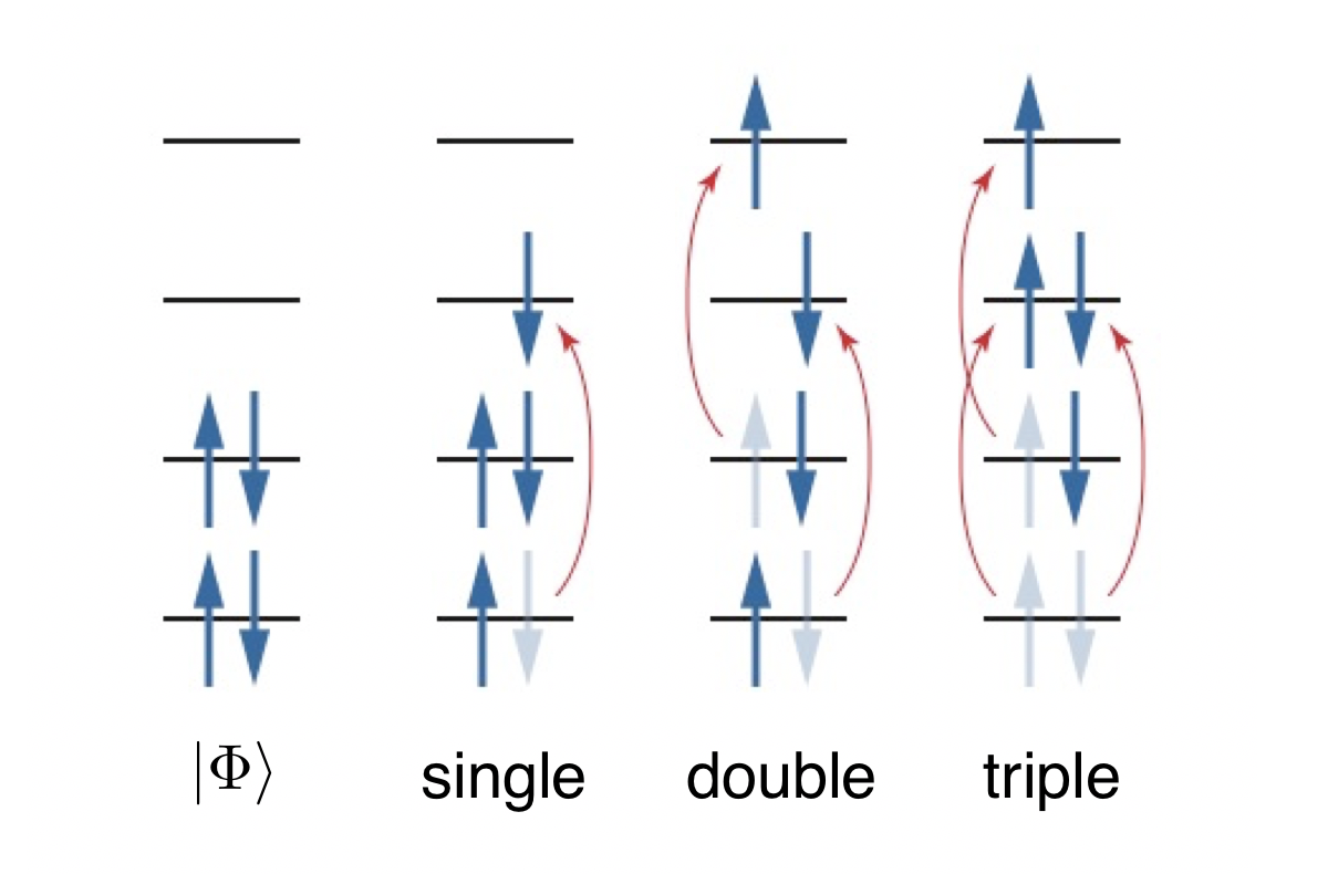
Classical CC methods have been used to compute the impurity coupled cluster Green’s function (CCGF) [24, 25, 26] both for the AIM and other Green’s function schemes for solving impurity models [38, 34]. The CC approach solves the corresponding many-body problem by considering a subset of excitations from a reference state [9, 10, 8, 27, 31]. This method becomes exact in the limit that all possible excitations are considered; however, the computational complexity grows polynomially in the system size and factorially in the number of excited particles considered. Typical implementations use the Hartree-Fock solution as a reference and truncate the possible excitations to single-, double-, and sometimes triple-particle excitations (see. Fig. 1). These implementations achieve for CCGF based on single and double excitations and when triple excitations are added. This scaling is a significant improvement over the exponential scaling of methods like exact diagonalizaton and its non-exact variants like the Lanczos algorithm, or quantum Monte Carlo methods applied to models with a sign problem. However, for strongly correlated regimes, where many-body effect become significant, one often needs to go beyond triple excitations to obtain converged solutions [3]. In this regime, classical algorithms for computing reliable CCGFs in either the frequency or time domain become severely constrained by memory and storage requirements [6, 28, 29, 35].
As with the classical CC algorithm, our hybrid quantum-classical algorithm for calculating the Green’s function requires a reference state ; however, we have found that we can obtain accurate results for the AIM using a simple product state. This aspect replaces the need for preparing a more complicated ground state on a quantum computer with a simpler task of applying unitary operators to a product state. To achieve this, we use the single CC amplitude obtained from fully converged classical CC calculations to construct the quantum measurement of the time-evolved unitary components of the non-Hermitian CCGF. This scheme allows us to extract the value of the Green’s function in the time domain. Using quantum computing algorithms for unitary time dynamics, our formalism can then calculate the impurity Green’s function of our benchmark AIM model at time to precision with a total -gate cost of
Here, is the probability of failing to properly implement the linear combination of unitary operators, is the synthesis error introduced by the time evolution operator, is the total evolution time, is the number of continuum energy levels (or “bath sites”) in the AIM, is the error introduced by the measurement scheme used, and is a constant dependent on the parameters of the AIM.
2 Methods
2.1 The Anderson Impurity Model
Our CC method is broadly applicable to many fermionic models of interest. Here, we demonstrate and benchmark our approach using the AIM [2], which has played an essential role in developing our understanding of localized fermionic degrees of freedom coupled to a continuum [15, 20]. The model describes localized magnetic moments embedded in a sea of conduction electrons and is closely related to the Kondo problem [32, 15]. It also plays a central role in dynamical mean-field theory (DMFT) [14], where an infinite interacting system is mapped onto an AIM whose parameters are determined self-consistently to reproduce the physics of the original problem. (In the DMFT context, the continuum levels are often referred to as “bath” levels, and we will use this language throughout the paper.)
The Hamiltonian for the AIM is given by
| (1) | ||||
Here, is an energy level index, where corresponds to the impurity site and correspond to the energy levels of the continuum or bath, is the Coulomb repulsion on the impurity site, is the hybridization parameter that allows hopping between the bath and impurity levels, and are the on-site energies of each level.
2.2 Coupled Cluster Green’s Functions from a sum of Unitary Operators
Given a many-body system with a model Hamiltonian , our goal is to construct the time-dependent single-particle retarded (advanced) Green’s function [] with the error of at most . Here, we focus on the zero-temperature case, where the Green’s functions are given by
| (2) |
and
| (3) |
where is the fermionic annihilation operator in the Heisenberg representation and is the ground state of .
Our algorithm to compute or consists of three main components, which address ground state preparation, time evolution, and measurements. As discussed in the introduction, the bottleneck for many quantum or quantum- classical algorithms lies in preparing the ground state of the system. A novel aspect of our CC method is that it allows us to approximate the ground state by considering excitations from a simple product reference state . Specifically, the state is approximated by applying cluster operators to (as in classical CC methods), but the operators are approximated here by a linear combination of unitary operators, as described in greater detail below.
2.3 State Preparation
As described in Refs. 24, 25, 26, the CCGF is built upon the CC bi-variational exponential parametrization of the reference state for approaching the many-body ground-state wave function of a system
| (4) |
and its dual
| (5) |
where and are cluster (excitation) and de-excitation operators, respectively. In the language of second quantization, and are given by sum of multi-particle scattering operators
| (6) | ||||
Here, the indices () denote occupied (unoccupied) spin-orbitals in the reference , the coefficients ’s and ’s are scalar amplitudes, and is the excitation level ( number of electrons) that defines the approximation in the CC hierarchy (e.g. corresponds to CC singles and doubles (CCSD) [31], corresponds to CC singles, doubles, and triples (CCSDT) [23, 22, 33], etc., see Fig. 1).
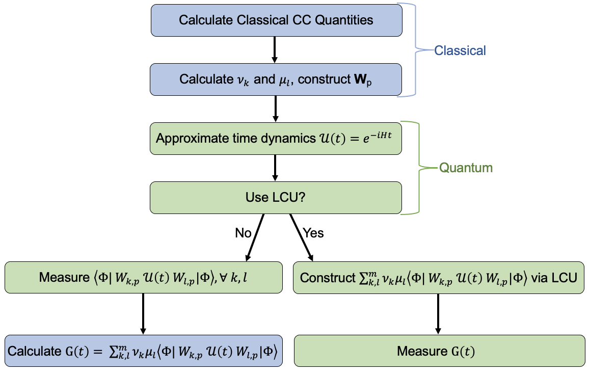
By employing the CC bi-variational parametrization, the time-dependent CCGF for a many-body electron system can be expressed as
| (7) |
where
| (8) |
and
| (9) |
Here, denotes the expectation value of an operator with respect to the reference . In the classical CCGF formulation, the operators appearing in Eqs. (8) and (9) are not unitary. This method must be modified for use on quantum computers, which require unitary operations.
We now illustrate how to develop a unitary formulation of the CC method using the lesser part [Eq. (8)]. Similar considerations apply to the greater term . We have found that at least one time-independent set of unitaries can be employed to expand and with the scalar coefficients and such that Eq. (8) can be fully unitarized. If we limit our discussion to the CCSD framework (i.e. , where for and , with and being the virtual and occupied subspace, respectively) and the index , then one option for is (see detailed derivation in A)
Here, denotes an Pauli operator (or gate) acting on the th spin-orbital (or qubit) with Pauli operators acting on all qubits before it in our ordering, and , where and denote the numbers of virtual and occupied spin-orbitals, respectively. The coefficients and are given by cluster amplitudes (see A). Note that the CCSD ground state energy for a general AIM with one impurity site only depends on the single amplitude, i.e. since the double amplitudes in a CCSD calculation of AIM are only used to converge the single amplitudes corresponding to the excitation from the impurity to the bath. Thus, if we only use the converged amplitude to construct (or approximate) the correlated wave function, the associated ground state energy will be exactly same as the CCSD correlation energy but the number of unitary vectors is greatly reduced from to .
Once the unitary set and time propagator operator are constructed, the lesser CCGF can be expressed as
| (10) |
where the expectation values are computed using a quantum device. In the case of the AIM, the lesser CCGF for the impurity site would correspond to . Note that the gate depth for is just , while the number of terms in Eq. (10) scales as . The method(s) for constructing the time evolution operator and measuring the expected values in Eq. (10) are discussed in the next two subsections.
In analogy to the single-reference CC formulations discussed above, one can map to other parametrizations of the ground wave function. For example, one can consider a unitary representation
| (11) |
where is an anti-Hermitian cluster operator, or multi-reference CC expansions
| (12) |
where the coefficients define the eigenvector of the effective Hamiltonian, are reference functions defining model space, and the operators are reference-specific cluster operators. If we choose a specific Slater determinant as a reference, other Slater determinants can be obtained as a , where the operator contains a string of creation/annihilation operators carrying active spin-orbital indices only.
2.4 Time evolution
There are multiple methods for approximating the time evolution operator. One option, which we adopt here, is to use a symmetrized Trotter formula with a Givens rotation, as described in Ref. 16. In this case, we separate the potential terms from the hopping terms and implement them separately as , as proposed in Ref. 16. By implementing a series of Givens rotations between the potential and hopping terms, the hopping terms become single qubit rotations, which must be synthesized using gates. Note that this Trotter decomposition will require two implementations of the set of Givens rotations, a set of rotations into the diagonal basis of the hopping Hamiltonian and a set of rotations back into the computational basis.
For more advanced simulation methods such as qubitization[19] and Taylor series expansion [5], oracles are required. They incur a cost based on query complexity, i.e. the number of times an oracle must be accessed to perform the simulation. These oracles must also be constructed using basic gates and ancilla qubits, thus increasing the gate count. However, it was recently shown that the most expensive oracle to implement in the Taylor series and Qubitization methods, the Select(H) oracle, can be implemented with just gates[36]. For a comparison of time evolution methods in terms of gate count, see Tab. 1.
| \rowcolor[HTML]EFEFEF Algorithm | Ref. | Ancilla Qubits | Query Complexity | Gate/Query | Total Gate Count |
|---|---|---|---|---|---|
| Trotter (Givens rotation) | 16 | 0 | - | - | |
| \rowcolor[HTML]EFEFEF Taylor Series | 5, 36 | ||||
| Qubitization | 19, 36 |
2.5 Measurement
Although the scaling of the number of measurements needed to calculate the Green’s function grows quadratically in the system size, the linear combination of the expectation values needed to calculate the impurity Green’s function can be calculated in one circuit using the linear combination of unitaries (LCU) method[7].
To implement a linear combination of unitary operators, LCU requires ancillary qubits. Using the LCU method to measure the Green’s function of the AIM thus requires , and the number of required ancilla qubits therefore grows as . From theorem 3 of Ref. 7, we know the probability of success for this method. Consider a linear combination of unitary operators , with , , and . Let . Then there exists a quantum algorithm that implements an operator proportional to with failure probability , where and are the probabilities of failure to add and subtract two terms, respectively. We utilize this method to measure each term in Eq. (10) with one circuit, thus reducing the measurement error.
To measure the entire Green’s function in the time-domain with just one circuit with LCU, we first construct the circuit that implements the LCU that is comprised of all of the terms in Eq. (10), and then measure the expectation value of the LCU operator with the Hadamard test. It is also possible to measure each expectation value in Eq. (10) by using the Hadamard test with each term in an independent circuit, and then combine them. The -gate counts for the LCU method and the direct Hadamard test are given in the Error Analysis and Gate Count Scaling section. Because the LCU method has a failure probability, it is possible that the direct Hadamard test could be advantageous in terms of gate count, even though it has poorer scaling with respect to the system size.
We now focus on computing the local Green’s function of the AIM. In this case, the circuit to measure the real part of in the time-domain via LCU is
where the qubit state of the ancilla register is prepared in a state determined by the coefficients of the LCU. The top single ancilla qubit is the one utilized for the Hadamard test. Finally, to measure the imaginary part of the expectation value instead of the real part as shown, one needs only to apply two single qubit gates to the ancilla qubit.
3 Results and Benchmarks
3.1 Two and Three-Site Examples
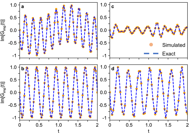
To demonstrate our method, we employed this hybrid quantum-classical algorithm to compute the many-body CCGF of AIM with and and compared our results with the exact solutions obtained with exact diagionalization.
For the case, we employ four qubits on the quantum simulator within the Qiskit framework[1]. We represent the model system with qubit #1 and #3 denoting the impurity site, and use a simple reference state . For the lesser CCGF, the set ( = 3) then only includes two elements , , such that is given by a linear combination of only three terms
| (13) | |||||
with the coefficient for each term determined from the product of the elements of and () as demonstrated in Eq. (10). The same strategy can be easily extended to an AIM with more bath levels. For example, for simulating a three-level model, six qubits can be employed to represent the model system with two qubits denoting the impurity site, and the trial state given by . In this case, computing the lesser CCGF Green’s function requires a set ( = 3) with six elements , , , , , , such that is given by a sum over twenty-one terms. However, based on our previous finding, these twenty-one terms can be reduced to just three terms related to only two elements of the set , . This reduction is due to the fact that the CCSD ground state energy for the AIM only depends on the single excitation cluster amplitudes.
To implement the time evolution operator in our examples, we separate the potential terms from the hopping terms and implement the former as a second order symmetric product formula. However, for our two and three-site examples, we do not implement the more advanced Trotter method with Givens rotations and instead implement the terms directly.
Figure 3 shows the impurity Green’s function in the time domain for the two- (Fig. 3a and 3b) and three-site (Fig. 3c and 3d) AIM. (In both cases, our simulations were conducted for parameters that typically arise in the DMFT self-consistency loop, along with a parameter set that corresponds to the final self-consistent solution.) We then fast-fourier transform (FFT) the time domain impurity Green’s function to the frequency domain to obtain the spectral functions , as shown in Fig. 4. For the three-site system, we tested the dependence of the solution on the number of Trotter steps taken per time step. We found that the results shown in Figs. 3c and 3d had little dependence on the number of Trotter steps taken for our choice of parameters and time step size. For example, data obtained for 8 and 32 Trotter steps per time step essentially coincide in Figs 3c and 3d. Here, the insensitivity of the solution on the number of Trotter steps is due to the small time step size we employed. In all cases, our hybrid quantum-classical algorithm reproduces the exact solution obtained by exact diagonalization.
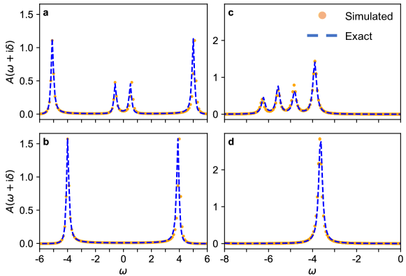
Although the examples of the two- and three-site Anderson impurity model are relatively simple, it is important to note that this method is very general. Here, we focused on the solutions of the two- and three-site problems for two sets of parameters (each) in order to emphasize that the efficacy of our approach does not depend strongly on the specific model parameters, even though the specifics of the model lead to simplifications in the method. It is also important to see the flexibility of the operators in the construction of any form of the -electron ground state wave functions.
4 Discussion
4.1 Advantages over VQE-based methods
Several VQE-based methods to calculate the Green’s function have been proposed in the literature. Ref. 17, for example, uses a unitary coupled cluster ansatz to prepare an approximation to the ground state, which is then used to generate transition matrix elements via statistical sampling. These transition matrix elements are then used in conjunction with the (known) pole locations (obtained via any one of a number of previously proposed algorithms for obtaining many-electron energy eigenvalues) to construct the Green’s function of the lithium hydride and water molecules. In a similar variational formulation, the authors of Ref. 11 utilize the VQE framework to calculate both the real-time Green’s functions and the Lehmann representation of the spectral function of a many-body system. To do this, the authors utilize VQE to construct the ground state, implement time evolution, find transition matrix elements, and obtain the many-electron energy eigenvalues needed in the Lehmann representation. As a numerical demonstration, they utilize the two-site Fermi-Hubbard model.
Our method differs from these VQE-based methods in many important ways. First, we do not require any prior determination of the many-electron energy eigenvalues. Instead, we work directly in the time domain and use a Fourier transform to obtain them. Second, our method does not rely on classical optimization algorithms, thus bypassing the so called “barren minima” problem that can occur in VQE solutions. Third, we have flexibility in the definition of the time-independent sets, which offers a tuning mechanism to the available quantum resources. The sets also allow for the definition of selective sub-sets of excitations to describe correlations in the -electron space. This freedom could be exploited in the construction of a subspace representation of the Green’s function, as is done in active-space formulations of ionization-potentials/electron-affinities equation-of-motion coupled-cluster methods.
Finally, the sets also provide great flexibility in emulating any form of the -electron ground-state wave functions, including higher-order coupled-cluster wave function expansions, configuration interaction representations, and multi-reference wave functions that may be required to handle strong correlation effects in the ground state. In this paper, we focused only on the single-reference CC parametrizations of the ground-state wave functions. From this perspective, the possibility of mapping arbitrary wave functions into the Pauli strings spanning the subspace defines the universal character of the proposed quantum algorithm in dealing with various many-body systems.
4.2 Error Analysis and Gate Count Scaling
Suppose we want to calculate the impurity Green’s function of an AIM with bath sites in the time domain, to within a total error for a total time . We consider two main contributions to , namely the synthesis error from implementing the time evolution operator, and due to statistical errors in the measurement scheme. Here, we propose utilizing LCU with the Hadamard test to measure the entire impurity Green’s function in the time domain with one circuit, using the Trotter (Givens rotations) method to approximate the time evolution operator. Alternatively, one could measure each expectation value in Eq. (10) separately with the Hadamard test, again using the Trotter (Givens rotation) method of Ref. 16 to approximate the time evolution operator. In our two-site example, we use the Hadamard test method for the convenience of implementation.
With the LCU method, for a given failure probability , measurement error tolerance , and number of gates required to implement the multiple controlled unitary operators, we need to use gates to successfully measure the full impurity Green’s function. Here, we use the convention that the variance in a single measurement is , and grows as with the number of samples taken. In this case, the number of ancilla qubits required to implement the LCU will grow as , plus one ancilla for the Hadamard test. Breaking the multiple controlled qubits into basis gates requires extra "work qubits," and the number of work qubits needed grows as the number of ancillas in the control register minus one. This additional requirement does not change the asymptotic scaling of the number of ancilla qubits required; it remains . (See, e.g. Ref. 21 for gate construction of the multiple controlled unitaries.)
To implement the multiple controlled version of each unitary within the LCU method, gates are required, where is the total evolution time and is a system-dependent factor from utilizing the Trotter decomposition of the time evolution operator. Implementing all multiple controlled unitaries then requires gates. Note, however, that each unitary will have some synthesis error due to the approximation of the time evolution operator and there will be time evolution operators in the full circuit. Therefore, to maintain a maximum synthesis error of , each time evolution operator can contribute no more than error. In the above expression, substituting gives a total gate scaling of . Thus, we have a full gate count of to measure the impurity Green’s function in the time domain. This implementation has the advantage of only requiring one circuit to measure with the Hadamard test.
If one uses the Hadamard test to measure each term in Eq. (10) separately, each controlled unitary will require gates. Since there are controlled unitaries to be implemented, this yields a gate complexity of . Since each unitary includes time evolution with some synthesis error, we again take . Similarly, for each of the unitary operators to be measured, the measurement error grows as , where is again the number of samples taken. Thus, to measure all of the terms to a total measurement error , total samples are required. Substituting gives a total gate scaling of .
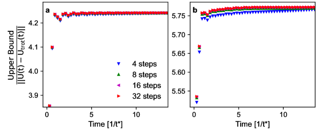
Figure 5 shows the ratio of the upper bound on the Trotter error from Ref. 16 to the actual Trotter error computed for our system in different parameter regimes for both the two and three-site systems. To obtain this figure, we compute the value of the factor directly and utilize the 2-norm of the operators equal to the largest singular value.
5 Conclusions
We have presented a hybrid quantum-classical approach for calculating time-domain Green’s functions of fermionic models based on coupled-cluster methods. Applying this approach to the AIM, we built a rigorous but straightforward fermion-to-unitary mapping for the non-unitary CCGF exponential operators. We then combined the cluster amplitudes calculated using the classical coupled-cluster algorithm with measurements of time-evolution operators on a quantum device to extract the impurity Green’s function in the real-time domain. On the quantum end, this approach replaces the need to prepare the ground state and can be easily generalized to many models. Our method has a T-gate count that scales as with no state preparation, if we use the LCU measurement scheme outlined here with the Trotter (Givens rotation) time evolution procedure.
We demonstrated the accuracy of our approach for the two- and three-level AIM models on a quantum simulator, where we obtained results in excellent agreement with the exact solutions. Further complexity analysis of the employed second-order symmetric time-evolution operator indicates that our method has comparable scaling of the gate counts (as a function of system size) in comparison with other state-of-the-art time evolution schemes. Our work provides a novel strategy for calculating the time-domain impurity Green’s function using a controlled approximation for the ground state wave function. This approach could be beneficial for situations where we know little about the ground state of the system or when the system’s spectral gap is small.
References
- Aleksandrowicz et al. [2019] Gadi Aleksandrowicz, Thomas Alexander, Panagiotis Barkoutsos, Luciano Bello, Yael Ben-Haim, David Bucher, Francisco Jose Cabrera-Hernández, Jorge Carballo-Franquis, Adrian Chen, Chun-Fu Chen, Jerry M. Chow, Antonio D. Córcoles-Gonzales, Abigail J. Cross, Andrew Cross, Juan Cruz-Benito, Chris Culver, Salvador De La Puente González, Enrique De La Torre, Delton Ding, Eugene Dumitrescu, Ivan Duran, Pieter Eendebak, Mark Everitt, Ismael Faro Sertage, Albert Frisch, Andreas Fuhrer, Jay Gambetta, Borja Godoy Gago, Juan Gomez-Mosquera, Donny Greenberg, Ikko Hamamura, Vojtech Havlicek, Joe Hellmers, Łukasz Herok, Hiroshi Horii, Shaohan Hu, Takashi Imamichi, Toshinari Itoko, Ali Javadi-Abhari, Naoki Kanazawa, Anton Karazeev, Kevin Krsulich, Peng Liu, Yang Luh, Yunho Maeng, Manoel Marques, Francisco Jose Martín-Fernández, Douglas T. McClure, David McKay, Srujan Meesala, Antonio Mezzacapo, Nikolaj Moll, Diego Moreda Rodríguez, Giacomo Nannicini, Paul Nation, Pauline Ollitrault, Lee James O’Riordan, Hanhee Paik, Jesús Pérez, Anna Phan, Marco Pistoia, Viktor Prutyanov, Max Reuter, Julia Rice, Abdón Rodríguez Davila, Raymond Harry Putra Rudy, Mingi Ryu, Ninad Sathaye, Chris Schnabel, Eddie Schoute, Kanav Setia, Yunong Shi, Adenilton Silva, Yukio Siraichi, Seyon Sivarajah, John A. Smolin, Mathias Soeken, Hitomi Takahashi, Ivano Tavernelli, Charles Taylor, Pete Taylour, Kenso Trabing, Matthew Treinish, Wes Turner, Desiree Vogt-Lee, Christophe Vuillot, Jonathan A. Wildstrom, Jessica Wilson, Erick Winston, Christopher Wood, Stephen Wood, Stefan Wörner, Ismail Yunus Akhalwaya, and Christa Zoufal. Qiskit: An Open-source Framework for Quantum Computing, January 2019. URL https://doi.org/10.5281/zenodo.2562111.
- Anderson [1961] P. W. Anderson. Localized magnetic states in metals. Phys. Rev., 124:41–53, Oct 1961. doi: 10.1103/PhysRev.124.41.
- Bartlett and Musiał [2007] Rodney J. Bartlett and Monika Musiał. Coupled-cluster theory in quantum chemistry. Rev. Mod. Phys., 79:291–352, Feb 2007. doi: 10.1103/RevModPhys.79.291.
- Bauer et al. [2016] Bela Bauer, Dave Wecker, Andrew J. Millis, Matthew B. Hastings, and Matthias Troyer. Hybrid quantum-classical approach to correlated materials. Physical Review X, 6(3):1–11, 2016. ISSN 21603308. doi: 10.1103/PhysRevX.6.031045.
- Berry et al. [2015] Dominic W Berry, Andrew M Childs, Richard Cleve, Robin Kothari, and Rolando D Somma. Simulating Hamiltonian Dynamics with a Truncated Taylor Series. Phys. Rev. Lett., 114(9):90502, mar 2015. doi: 10.1103/PhysRevLett.114.090502.
- Bhaskaran-Nair et al. [2016] Kiran Bhaskaran-Nair, Karol Kowalski, and William A. Shelton. Coupled cluster green function: Model involving single and double excitations. J. Chem. Phys., 144(14):144101, 2016. doi: http://dx.doi.org/10.1063/1.4944960.
- Childs and Wiebe [2012] Andrew M. Childs and Nathan Wiebe. Hamiltonian simulation using linear combinations of unitary operations. Quantum Information and Computation, 12(11-12):901–924, 2012. ISSN 15337146. doi: 10.26421/QIC12.11-12.
- Čížek [1966] J. Čížek. On the correlation problem in atomic and molecular systems. calculation of wavefunction components in Ursell-type expansion using quantum-field theoretical methods. J. Chem. Phys., 45(11):4256–4266, 1966. doi: http://dx.doi.org/10.1063/1.1727484.
- Coester [1958] F. Coester. Bound states of a many-particle system. Nucl. Phys., 7:421–424, 1958. ISSN 0029-5582. doi: http://dx.doi.org/10.1016/0029-5582(58)90280-3.
- Coester and Kümmel [1960] F. Coester and H. Kümmel. Short-range correlations in nuclear wave functions. Nucl. Phys., 17:477–485, 1960. ISSN 0029-5582. doi: http://dx.doi.org/10.1016/0029-5582(60)90140-1.
- Endo et al. [2020a] Suguru Endo, Iori Kurata, and Yuya O. Nakagawa. Calculation of the Green’s function on near-term quantum computers. Phys. Rev. Research, 2:033281, Aug 2020a. doi: 10.1103/PhysRevResearch.2.033281.
- Endo et al. [2020b] Suguru Endo, Iori Kurata, and Yuya O. Nakagawa. Calculation of the Green’s function on near-term quantum computers. Phys. Rev. Research, 2:033281, Aug 2020b. doi: 10.1103/PhysRevResearch.2.033281.
- Georges and Kotliar [1992] Antoine Georges and Gabriel Kotliar. Hubbard model in infinite dimensions. Phys. Rev. B, 45:6479–6483, Mar 1992. doi: 10.1103/PhysRevB.45.6479.
- Georges et al. [1996] Antoine Georges, Gabriel Kotliar, Werner Krauth, and Marcelo J. Rozenberg. Dynamical mean-field theory of strongly correlated fermion systems and the limit of infinite dimensions. Reviews of Modern Physics, 68(1):13–125, 1996. ISSN 1526498X. doi: 10.1103.
- Hewson [1993] A.C. Hewson. The Kondo Problem to Heavy Fermions. Cambridge Studies in Magnetism, Vol. 2. Cambridge University Press, Cambridge, 1993.
- Kivlichan et al. [2020] Ian D. Kivlichan, Craig Gidney, Dominic W. Berry, Nathan Wiebe, Jarrod McClean, Wei Sun, Zhang Jiang, Nicholas Rubin, Austin Fowler, Alán Aspuru-Guzik, Hartmut Neven, and Ryan Babbush. Improved Fault-Tolerant Quantum Simulation of Condensed-Phase Correlated Electrons via Trotterization. Quantum, 4:296, 2020. ISSN 2521-327X. doi: 10.22331/q-2020-07-16-296.
- Kosugi and Matsushita [2020] Taichi Kosugi and Yu-ichiro Matsushita. Construction of Green’s functions on a quantum computer: Quasiparticle spectra of molecules. Phys. Rev. A, 101:012330, Jan 2020. doi: 10.1103/PhysRevA.101.012330.
- Lin and Tong [2020] Lin Lin and Yu Tong. Near-optimal ground state preparation. Quantum, 4:372, December 2020. ISSN 2521-327X. doi: 10.22331/q-2020-12-14-372.
- Low and Chuang [2019] Guang Hao Low and Isaac L. Chuang. Hamiltonian Simulation by Qubitization. Quantum, 3:163, 2019. ISSN 2521-327X. doi: 10.22331/q-2019-07-12-163.
- Mahan [1990] G.D. Mahan. Many-Particle Physics. Physics of Solids and Liquids. Springer US, 1990. ISBN 9780306434235.
- Nielsen and Chuang [2011] Michael A. Nielsen and Isaac L. Chuang. Quantum Computation and Quantum Information: 10th Anniversary Edition. Cambridge University Press, New York, NY, USA, 10th edition, 2011. ISBN 1107002176, 9781107002173.
- Noga and Bartlett [1988] J. Noga and R. J. Bartlett. Erratum: The full ccsdt model for molecular electronic structure [j. chem. phys. 86, 7041 (1987)]. J. Chem. Phys., 89(5):3401–3401, 1988. doi: 10.1063/1.455742.
- Noga and Bartlett [1987] Jozef Noga and Rodney J. Bartlett. The full ccsdt model for molecular electronic structure. J. Chem. Phys., 86(12):7041–7050, 1987. doi: 10.1063/1.452353.
- Nooijen and Snijders [1992] Marcel Nooijen and Jaap G. Snijders. Coupled cluster approach to the single-particle Green’s function. Int. J. Quantum Chem., 44(S26):55–83, 1992. ISSN 1097-461X. doi: 10.1002/qua.560440808.
- Nooijen and Snijders [1993] Marcel Nooijen and Jaap G. Snijders. Coupled cluster Green’s function method: Working equations and applications. Int. J. Quantum Chem., 48(1):15–48, 1993. ISSN 1097-461X. doi: 10.1002/qua.560480103.
- Nooijen and Snijders [1995] Marcel Nooijen and Jaap G. Snijders. Second order many-body perturbation approximations to the coupled cluster Green’s function. J. Chem. Phys., 102(4):1681–1688, 1995. doi: http://dx.doi.org/10.1063/1.468900.
- Paldus et al. [1972] J. Paldus, J. Čížek, and I. Shavitt. Correlation problems in atomic and molecular systems. IV. Extended coupled-pair many-electron theory and its application to the B molecule. Phys. Rev. A, 5:50–67, Jan 1972. doi: 10.1103/PhysRevA.5.50.
- Peng and Kowalski [2018] Bo Peng and Karol Kowalski. Green’s function coupled-cluster approach: Simulating photoelectron spectra for realistic molecular systems. J. Chem. Theory Comput., 14(8):4335–4352, 2018. doi: 10.1021/acs.jctc.8b00313.
- Peng et al. [2019] Bo Peng, Roel Van Beeumen, David B. Williams-Young, Karol Kowalski, and Chao Yang. Approximate Green’s function coupled cluster method employing effective dimension reduction. Journal of Chemical Theory and Computation, 15(5):3185–3196, 2019. doi: 10.1021/acs.jctc.9b00172. PMID: 30951302.
- Peruzzo et al. [2014] Alberto Peruzzo, Jarrod McClean, Peter Shadbolt, Man Hong Yung, Xiao Qi Zhou, Peter J. Love, Alán Aspuru-Guzik, and Jeremy L. O’Brien. A variational eigenvalue solver on a photonic quantum processor. Nature Communications, 5(May), 2014. ISSN 20411723. doi: 10.1038/ncomms5213.
- Purvis and Bartlett [1982] G. Purvis and R. Bartlett. A full coupled-cluster singles and doubles model: The inclusion of disconnected triples. J. Chem. Phys., 76(4):1910–1918, 1982. doi: http://dx.doi.org/10.1063/1.443164.
- Schrieffer and Wolff [1966] J. R. Schrieffer and P. A. Wolff. Relation between the Anderson and Kondo Hamiltonians. Phys. Rev., 149:491–492, Sep 1966. doi: 10.1103/PhysRev.149.491.
- Scuseria and Schaefer [1988] Gustavo E. Scuseria and Henry F. Schaefer. A new implementation of the full ccsdt model for molecular electronic structure. Chem. Phys. Lett., 152(4):382–386, 1988. ISSN 0009-2614. doi: https://doi.org/10.1016/0009-2614(88)80110-6.
- Shee and Zgid [2019] Avijit Shee and Dominika Zgid. Coupled cluster as an impurity solver for Green’s function embedding methods. Journal of Chemical Theory and Computation, 15(11):6010–6024, 2019. doi: 10.1021/acs.jctc.9b00603. PMID: 31518129.
- Vila et al. [2020] F. D. Vila, J. J. Rehr, J. J. Kas, K. Kowalski, and B. Peng. Real-time coupled-cluster approach for the cumulant Green’s function. Journal of Chemical Theory and Computation, 16(11):6983–6992, 2020. doi: 10.1021/acs.jctc.0c00639. PMID: 33108872.
- Wan [2021] Kianna Wan. Exponentially faster implementations of select(h) for fermionic hamiltonians. Quantum, 5:380, Jan 2021. ISSN 2521-327X. doi: 10.22331/q-2021-01-12-380.
- Wecker et al. [2015] Dave Wecker, Matthew B. Hastings, and Matthias Troyer. Progress towards practical quantum variational algorithms. Physical Review A - Atomic, Molecular, and Optical Physics, 92(4):1–11, 2015. ISSN 10941622. doi: 10.1103/PhysRevA.92.042303.
- Zhu et al. [2019] Tianyu Zhu, Carlos A. Jiménez-Hoyos, James McClain, Timothy C. Berkelbach, and Garnet Kin-Lic Chan. Coupled-cluster impurity solvers for dynamical mean-field theory. Phys. Rev. B, 100:115154, Sep 2019. doi: 10.1103/PhysRevB.100.115154.
Acknowledgements: We thank E. F. Dumitrescu for useful discussions. T. K. is supported by the U. S. Department of Energy, Office of Science, Office of Workforce Development for Teachers and Scientists, Office of Science Graduate Student Research (SCGSR) program. The SCGSR program is administered by the Oak Ridge Institute for Science and Education (ORISE) for the DOE. ORISE is managed by ORAU under contract number DE-SC0014664. All opinions expressed in this paper are the author’s and do not necessarily reflect the policies and views of DOE, ORAU, or ORISE. This work was performed in part at Oak Ridge National Laboratory, operated by UT-Battelle for the U.S. Department of Energy under Contract No. DE-AC05-00OR22725. B. P. and K. K. were supported by the “Embedding QC into Many-body Frameworks for Strongly Correlated Molecular and Materials Systems” project, which is funded by the U. S. Department of Energy, Office of Science, Office of Basic Energy Sciences (BES), the Division of Chemical Sciences, Geosciences, and Biosciences. B. P. also acknowledges the support of Laboratory Directed Research and Development (LDRD) program from PNNL. T. K. and P. L. were supported by the U. S. Department of Energy, Office of Science, Office of Advanced Scientific Computing Research (ASCR) Quantum Algorithm Teams (QAT) and Quantum Computing Application Teams (QCATS) programs, under field work proposal numbers ERKJ333 and ERKJ347.
Author Contributions: T. K., B. P., K. K., and P. L. designed the study, T. K. and B. P. collected data, and produced figures. S. J. developed a classical exact diagionalization code for the AIM. B. P., K. K., and P. L., supervised the research. All authors discussed the results and contributed to the final paper.
Competing Interests: The authors declare no competing interests.
Data availability: The data supporting this study are available at https://doi.org/10.5281/zenodo.5920664.
Code availability: The code used to obtain the coupled-cluster quantities is available at https://github.com/spec-org/gfcc. The code used for the quantum-classical algorithm is available at https://doi.org/10.5281/zenodo.5920664.
Appendix A Finding Unitaries and scalar coefficients .
If index denotes impurity site, then one option of can be obtained through the Jordan-Wigner mapping of the transformed . Here, we use the Jordan-Wigner transformation given by
| (14) |
where the first qubits hold the down occupation information for each site, and the second qubits hold the up occupation information for each site. In the CCSD approximation, this can be expressed as
where . The can then be chosen as , and the scalars are the corresponding cluster amplitudes in (A). can be expanded by the same set with the corresponding scalars given by
Similarly, we can transform ,
to get another set of unitaries and corresponding scalars for greater part of the coupled cluster Green’s function.
It is worth mentioning that the cluster amplitudes, ’s, in the present context are obtained from classical CCSD calculation on AIM, which numerically scales ( denoting the number of occupied spin-orbitals and denoting the number of virtual spin-orbitals).
