Jet Angularities in Z+jet production at the LHC

Abstract

We present a phenomenological study of angularities measured on the highest transverse-momentum jet in LHC events that feature the associate production of a $Z$ boson and one or more jets. In particular, we study angularity distributions that are measured on jets with and without the SoftDrop grooming procedure. We begin our analysis exploiting state-of-the-art Monte Carlo parton shower simulations and we quantitatively assess the impact of next-to-leading order (NLO) matching and merging procedures. We then move to analytic resummation and arrive at an all-order expression that features the resummation of large logarithms at next-to-leading logarithmic accuracy (NLL) and is matched to the exact NLO result. Our predictions include the effect of soft emissions at large angles, treated as a power expansion in the jet radius, and non-global logarithms. Furthermore, matching to fixed-order is performed in such a way to ensure what is usually referred to as NLL^′ accuracy. Our results account for realistic experimental cuts and can be easily compared to upcoming measurements of jet angularities from the LHC collaborations.

1 Introduction

During the first two runs of the CERN Large Hadron Collider (LHC) the experimental collaborations have accumulated a vast amount of high-quality data of proton–proton collisions at energies as high as $13$ TeV. In the current shutdown period, the collaborations refine their search and measurement strategies, in order to fully exploit the physics potential of the acquired data, and to prepare for the upcoming third run of the LHC. However, no significant increase in collision energy is planned for the foreseeable future. Accordingly, the focus of the theory and experimental communities should be on devising new effective and robust analysis techniques to interrogate the data, so that no stone is left unturned. In this context, the use of deep-learning algorithms to augment performance is now becoming standard practice (see e.g. (Larkoski:2017jix, ; Kasieczka:2019dbj, ; Benato:2020sbi, ) for recent reviews). Complementary to this effort, measurement campaigns that deliver unfolded data that can be compared to state-of-the-art theoretical calculations have been, and will further be, pursued in order to stress-test our understanding of the Standard Model.

The physics of jets and their structure plays a special role in this effort. First of all, jets, i.e. collimated sprays of particles, are ubiquitous objects in hadronic-collision events. Furthermore, in experimental analyses, jets can be used in the context of searches for new physics, but also as a probe of strong-interaction phenomena and dynamics. Measurements of jet cross sections provide stringent tests of our understanding of the strong interaction, ranging over several orders of magnitude in the relevant energy scales. High-quality jet data are used in fits for the strong coupling constant, see e.g. (Britzger:2017maj, ; Chatrchyan:2013txa, ; Aaboud:2017fml, ; ATLAS:2015yaa, ; CMS:2014mna, ) and form an important input for constraining parton distribution functions (PDFs) (Aad:2021zrv, ; Aad:2013lpa, ; Khachatryan:2014waa, ; Khachatryan:2016mlc, ; AbdulKhalek:2020jut, ; Harland-Lang:2017ytb, ; Pumplin:2009nk, ; Watt:2013oha, ).

An accurate description of jets and their structure poses numerous theoretical challenges. Despite the fact that $2\to 2$ processes involving either two jets or a jet and an electroweak gauge boson are known to next-to-next-to-leading order (NNLO) accuracy in the strong coupling expansion, the presence of multiple scales, such as the jet transverse momentum, the jet radius and the substructure variables we would like to consider, e.g. the jet mass, renders fixed-order predictions in QCD insufficient. In order to achieve higher precision, fixed-order results need to be combined with resummed calculations. However, all-order evaluations of jet substructure observables are far from trivial due to the presence of hard boundaries in phase space, which give rise to non-global effects (Dasgupta:2001sh, ; Dasgupta:2002bw, ), and because of the algorithmic nature of jet definitions that make all-order factorisations difficult to achieve. These challenges have been tackled by the theory community over the past decade and nowadays, thanks to numerous QCD studies, e.g. (Dasgupta:2013ihk, ; Dasgupta:2013via, ; Larkoski:2014wba, ; Dasgupta:2015lxh, ; Salam:2016yht, ; Dasgupta:2016ktv, ; Dasgupta:2015yua, ; Larkoski:2014gra, ; Larkoski:2015kga, ; Larkoski:2020wgx, ; Larkoski:2013eya, ; Kang:2019prh, ; Cal:2019gxa, ; Cal:2020flh, ), a deeper understanding of jet substructure has been reached. One of the lessons we have learnt from these investigations is that so-called grooming techniques, i.e. jet substructure algorithms that aim to clean up a jet by removing from its constituents the ones that originate from soft physics, actually improve our ability to use perturbation theory to describe jet physics. They reduce the impact of non-perturbative effects due to hadronisation and the underlying event (UE), for a recent review, see e.g. (Marzani:2019hun, ). Furthermore, the all-order structure of the perturbative result is also simplified because groomers, such as the modified-MassDrop/SoftDrop algorithm (Dasgupta:2013ihk, ; Larkoski:2014wba, ), can eliminate the logarithmic enhancement due to soft gluons at wide angles, including the intricate structure of non-global logarithms by turning logarithms of the observable under consideration into logarithms of an external parameter, such as $z_{\text{cut}}$ in the case of SoftDrop .

In this study we concentrate on high-energy proton–proton collisions that result in the production of an electroweak $Z$ boson (decaying into a pair of muons) in association with one or more jets. For the jet with the highest transverse momentum, we are going to consider jet angularity observables (Larkoski:2014pca, ), which are variables that probe the energy flow within a jet. Prior to the angularity evaluation we optionally perform the SoftDrop procedure on the candidate jet. The considered jet angularities form an interesting testbed for our theoretical understanding of intra-jet QCD dynamics. Furthermore, they over great application potential, e.g. in distinguishing quark-like from gluon-like jets, in a theoretically well-defined way (Badger:2016bpw, ; Gras:2017jty, ; Amoroso:2020lgh, ), or in extractions of the strong coupling constant (Bendavid:2018nar, ). Our analysis begins with a detailed phenomenological study of jet angularities, which is performed exploiting state-of-the-art Monte Carlo (MC) parton shower simulations. Beside assessing the relative importance of the different contributions that affect the angularity distributions, such as perturbative radiation, hadronisation and the UE, our studies aim to quantify the role of modern NLO merging techniques on jet substructure distributions. We then move to the second part of the paper, where we present first-principle theoretical predictions for the observables of interest. Our resummed calculation is performed at next-to-leading logarithmic accuracy (NLL) matched to fixed-order predictions evaluated at NLO in $\alpha_{s}$. Furthermore, by keeping track of the jet flavour in our matching procedure, we are able to obtain what is usually referred to as $\text{NLL}^{\prime}$ accuracy. We stress that such accuracy is achieved for both the groomed and the ungroomed distributions, which implies that we account for single-logarithmic corrections originating from soft emissions at wide angle, that we treat as an expansion in the jet radius parameter, and from non-global logarithms, in the limit of large number of colours ($N_{c}$). Furthermore, our initial detailed study of MC predictions allows us to supplement our perturbative $\text{NLO}+\text{NLL}^{\prime}$ predictions with non-perturbative corrections extracted from hadron-level MC simulations. Our theoretical predictions are fully differential in the kinematics of the jets and of the leptonic decay products of the $Z$ boson, so that we can impose realistic fiducial cuts and compare them to the distributions obtained from MC event generators. Our predictions are obtained with the resummation plugin of the S HERPA generator framework (Gerwick:2014gya, ) and they can be directly compared to unfolded measurements from the LHC collaborations, once these become available.

The paper is organised as follows: in Section 2 we introduce the class of angularity observables to consider and detail our event selection cuts. In Section 3 we present and compare hadron-level predictions for groomed and ungroomed jet angularities from the H ERWIG and P YTHIA event generators, based on the leading-order matrix elements, and S HERPA , using multijet merging at leading and next-to-leading order. Section 4 is devoted to the all-orders evaluation of jet angularities at $\text{NLO}+\text{NLL}^{\prime}$ accuracy using the S HERPA resummation framework. In Section 5 we compare our resummed predictions with the parton-level results of our MC simulations. We extract non-perturbative corrections from the full particle-level simulations and apply them to our $\text{NLO}+\text{NLL}^{\prime}$ predictions. Our conclusions are presented in Section 6. Additional results are collected in Appendix A.

2 Observable definition

In this study we concentrate on the production of a leptonically decaying $Z$ boson associated with one or more jets at the LHC. Jets are defined using the anti-$k_{t}$ clustering algorithm (Cacciari:2008gp, ) with radius parameter $R_{0}$ and standard $E$-scheme recombination, i.e. the momenta of objects that are paired together are simply added so that the resulting jet momentum is given by the sum of its constituents’ momenta.

On the hardest jet, i.e. the jet with the largest transverse momentum $p_{T,\text{jet}}$, we measure the angularities (Berger:2003iw, ; Almeida:2008yp, ; Larkoski:2014pca, )

$$\lambda_{\alpha}^{\kappa}=\sum_{i\in\text{jet}}\mathopen{}\mathclose{{}\left(\frac{p_{T,i}}{\sum_{j\in\text{jet}}p_{T,j}}}\right)^{\kappa}\mathopen{}\mathclose{{}\left(\frac{\Delta_{i}}{R_{0}}}\right)^{\alpha}\,,$$ (1)

where

$$\Delta_{i}=\sqrt{(y_{i}-y_{\text{jet}})^{2}+(\phi_{i}-\phi_{\text{jet}})^{2}}\,,$$ (2)

is the Euclidean azimuth-rapidity distance of particle $i$ from the jet axis. Our study is limited to a subset of the above defined general angularities, namely the ones that exhibit infrared and collinear (IRC) safety. This poses the restrictions $\kappa=1$ and $\alpha>0$. Furthermore, it is well-known (Banfi:2004yd, ; Larkoski:2013eya, ) that IRC safe angularities with $\alpha\leq 1$ are sensitive to recoil against soft emissions, leading to a rather complicated resummation structure. To circumvent these additional complications, we compute for these angularities the distance measure in Eq. (2) with respect to the jet axis obtained by reclustering the jet constitutents with the anti-$k_{t}$ algorithm but using the Winner-Take-All (WTA) recombination scheme (Larkoski:2014uqa, ). We are also interested in computing angularities on groomed jets. In this case, we recluster the jet with the Cambridge–Aachen (C/A) algorithm and consider the SoftDrop grooming algorithm with parameters $z_{\rm cut}$ and $\beta$ (Larkoski:2014wba, ). The angularity is then computed on the resulting SoftDrop jet, i.e. both sums in Eq. (1) are restricted to the particles that survived the grooming. For groomed jets we also adopt the WTA prescription for angularities with $\alpha\leq 1$.

In order to highlight the behaviour of the angularity distributions in different energy regimes, standard and groomed angularities are considered in different jet transverse momentum bins. This will allow us, for instance, to better study the impact of non-perturbative corrections, e.g. from the parton-to-hadron transition. We note that, in order to avoid issues related to bin-migration, which greatly complicates the structure of the resummation of the SoftDrop $\beta=0$ (modified MassDrop) angularities (Marzani:2017mva, ), we shall always choose the reference transverse momentum $p_{T,\text{jet}}$ to be the one before grooming. Our theoretical predictions, both the ones obtained with matrix-element improved parton showers and with all-order resummation matched to fixed-order calculations, account for fiducial cuts and therefore can directly be compared to unfolded measurements.

Event selection cuts

We close this section by detailing the fiducial volume for the jets and leptons in our subsequent studies. Our choices follow the selection of a recent (preliminary) CMS measurement CMS-PAS-SMP-20-010 . We consider the inclusive production of a pair of oppositely charged muons in proton–proton collisions at $13~{}\text{TeV}$ centre-of-mass energy. We require all final state particles to have pseudo-rapidity $|\eta|<5$. For both muon candidates we require

$$p_{T,\mu}>26~{}\mathrm{GeV}\,,\;\;\text{and}\;\;|\eta_{\mu}|<2.4\,.$$ (3)

The lepton pair has to pass the additional conditions

$$\quad 70~{}\mathrm{GeV}<m_{\mu^{+}\mu^{-}}<110~{}\mathrm{GeV}\,,\;\;\text{and}\;\;p_{T,\mu^{+}\mu^{-}}>30\;\text{GeV}\,.$$ (4)

In what follows we will refer to the lepton pair as $Z$ boson, where nevertheless we imply the inclusion of off-shell effects. We then select events that exhibit at least one anti-$k_{t}$ jet (Cacciari:2008gp, ) with

$$|y_{\text{jet}}|<1.7\,,\quad\text{and}\quad R_{0}=0.8~{},$$ (5)

and consider several bins in $p_{T,\text{jet}}$ starting at $50~{}\text{GeV}$ following CMS-PAS-SMP-20-010 . We compiled results for all bins used there, but will in the following limit the discussion to $p_{T,\text{jet}}\in[120,150]~{}\text{GeV}$ and $p_{T,\text{jet}}\in[408,1500]~{}\text{GeV}$ that we find representative for the lower and higher jet scale selections. In order to gain better control over NLO QCD corrections for the $Zj$ production process, that become large when the $Z$-boson transverse momentum is significantly smaller than $p_{T,\text{jet}}$ (Rubin:2010xp, ), we require the transverse momenta of the lepton pair and the leading jet to be largely balanced. To this end we impose the constraint

$$\Delta^{p_{T}}_{Z,{\rm jet}}\equiv\mathopen{}\mathclose{{}\left|\frac{p_{T,\rm jet}-p_{T,\mu^{+}\mu^{-}}}{p_{T,\rm jet}+p_{T,\mu^{+}\mu^{-}}}}\right|<0.3\,.$$ (6)

Finally, we require the $Z$-boson and the leading jet to be well separated in azimuthal angle, i.e.

$$\Delta^{\phi}_{Z,{\rm jet}}\equiv\mathopen{}\mathclose{{}\left|\phi_{Z}-\phi_{\rm jet}}\right|>2\,.$$ (7)

In our following studies we will consider the jet angularities $\lambda_{\alpha}^{\kappa}$ with $\mathopen{}\mathclose{{}\left(\kappa,\alpha}\right)=(1,1/2),\,(1,1)$ and $(1,2)$. In previous studies (Larkoski:2014pca, ; Badger:2016bpw, ) these have been dubbed Les Houches Angularity (LHA) $\lambda^{1}_{1/2}$, Width $\lambda^{1}_{1}$, and Thrust $\lambda^{1}_{2}$, respectively. We adopt this naming convention here. For SoftDrop grooming we use $\beta=0$, $z_{\text{cut}}=0.1$ throughout.

3 State-of-the-art Monte Carlo study of jet angularities

The Born-level contributions to $Zj$ production are given by the two channels $pp\rightarrow\mu^{+}\mu^{-}+q/g$, where $q$ represents a massless quark or anti-quark. Jet angularities become non-trivial upon inclusion of additional radiation, which in general purpose MC generators is accounted for by parton shower simulations (Buckley:2011ms, ). However, to properly include non-logarithmic corrections, e.g. from hard real emissions, these should be matched to exact higher-order matrix elements, as obtained, for example using event generators such as M CFM  Campbell:1999ah ; Campbell:2011bn ; Boughezal:2016wmq , P OWHEG  Nason:2004rx ; Frixione:2007vw ; Alioli:2010xd or M ADGRAPH 5_aMC@NLO Frixione:2002ik ; Alwall:2014hca . Here we consider simulations including the complete set of NLO QCD corrections to the $Zj$ and $Zjj$ production processes matched to the S HERPA parton shower in the MEPS@NLO formalism (Hoeche:2012yf, ). To address the sensitivity of the angularities to non-perturbative corrections we also account for UE contributions to the collision final states and model the parton-to-hadron transition. In this section we describe the calculational setups for our Monte Carlo simulations and then present corresponding predictions for the groomed and ungroomed LHA, Width, and Thrust angularities.

3.1 Monte Carlo generator setup

We compile MC predictions for the jet angularities with the S HERPA  (Gleisberg:2008ta, ; Bothmann:2019yzt, ) event generator, version 2.2.10, using the NNPDF-3.0 NNLO PDF set (Ball:2014uwa, ). We consider the inclusive $Zj$ production process in the MEPS@NLO multijet merging formalism (Hoeche:2012yf, ), thereby combining the NLO QCD matrix elements for $\mu^{+}\mu^{-}j$ and $\mu^{+}\mu^{-}jj$ production, matched with the S HERPA Catani–Seymour dipole shower (Schumann:2007mg, ). We set the merging-scale parameter to $Q_{\text{cut}}=30\,\text{GeV}$ (which is of the order of the jet $p_{T}$ cut used in our event selection). We obtain the QCD one-loop amplitudes for the one- and two-jet processes from R ECOLA  (Actis:2016mpe, ; Biedermann:2017yoi, ), using the C OLLIER library (Denner:2016kdg, ) for the evaluation of tensor and scalar integrals. To assess the impact of the QCD one-loop corrections, we furthermore compile MEPS@LO (Hoeche:2009rj, ) predictions based on merging the one- and two-jet leading-order matrix elements, using $Q_{\text{cut}}=30\,\text{GeV}$ as well.

The perturbative scales entering the calculation are defined according to the CKKW-style scale setting prescription (Catani:2001cc, ; Hoeche:2009rj, ). In this procedure the hard-process partons are clustered into a Born-like $2\to 2$ configuration that defines the core process with an associated scale $\mu_{\text{core}}$. For the production channels considered here the event-wise determined core process, of order $\alpha_{\text{s}}^{n_{\text{core}}}$, can correspond to $jj\to\mu^{+}\mu^{-}$ ($n_{\text{core}}=0$), $jj\to Zj$ ($n_{\text{core}}=1$), or $jj\to jj$ ($n_{\text{core}}=2$). For the three possible cluster configurations the corresponding core-process scale is given by

$$\mu_{\text{core}}=\mathopen{}\mathclose{{}\left\{\begin{array}[]{lcl}m_{\mu^{+}\mu^{-}}&:&n_{\text{core}}=0\\ \sqrt{m^{2}_{\mu^{+}\mu^{-}}+p^{2}_{T,\mu^{+}\mu^{-}}}&:&n_{\text{core}}=1\;.\\ p_{T,j}&:&n_{\text{core}}=2\end{array}}\right.$$ (8)

The core-process scale is then used to define the factorisation scale and the parton shower starting scale of the core process, i.e.

$$\mu_{\text{F}}=\mu_{\text{core}}\,,\quad\mu_{\text{Q}}=R_{0}\mu_{\text{core}}\,.$$ (9)

Our choice of $\mu_{\text{Q}}$ here is motivated by the corresponding scale in the resummed calculation, c.f. Sec. 4. The effective renormalisation scale, $\mu_{\text{CKKW}}$, of the $n$-parton hard matrix elements corresponds to

$$\alpha_{\text{s}}^{n}(\mu^{2}_{\text{CKKW}})=\alpha_{\text{s}}^{n_{\text{core}}}(\mu^{2}_{\text{core}})\prod\limits_{i=1}^{n-n_{\text{core}}}\alpha_{\text{s}}(t_{i})\,,$$ (10)

with $t_{i}$ the reconstructed shower-branching scales. To estimate the perturbative uncertainties of our MC predictions, we do on-the-fly (Bothmann:2016nao, ) $7$-point variations (Cacciari:2003fi, ) of the factorisation and renormalisation scales in the matrix elements and the parton shower. The uncertainty bands given later on correspond to the envelope of the settings $\{(\tfrac{1}{2}\mu_{\text{R}},\tfrac{1}{2}\mu_{\text{F}})$, $(\tfrac{1}{2}\mu_{\text{R}},\mu_{\text{F}})$, $(\mu_{\text{R}},\tfrac{1}{2}\mu_{\text{F}})$, $(\mu_{\text{R}},\mu_{\text{F}})$, $(\mu_{\text{R}},2\mu_{\text{F}})$, $(2\mu_{\text{R}},\mu_{\text{F}})$, $(2\mu_{\text{R}},2\mu_{\text{F}})\}$.

To model the parton-to-hadron transition we use the S HERPA cluster fragmentation model (Winter:2003tt, ). The UE simulation relies on the S HERPA implementation of the Sjöstrand–Zijl multiple-parton interaction model (Sjostrand:1987su, ). In both models the default set of tuning parameters is used, see (Bothmann:2019yzt, ) for details.

To obtain further independent predictions, in particular for the modelling of non-perturbative effects, we compile additional results from H ERWIG  (Bellm:2015jjp, ; Bellm:2019zci, ), version 7.2.1, and P YTHIA  (Sjostrand:2014zea, ), version 8.303. For both generators we consider the $\mu^{+}\mu^{-}j$-production process at leading order, invoking the respective default models for the QCD parton shower, hadronisation and UE simulation.

For event selection and analysis we employ the R IVET analysis package (Buckley:2010ar, ; Bierlich:2019rhm, ). For jet reconstruction we use the F AST J ET  package (Cacciari:2011ma, ). For the SoftDrop grooming we rely on the implementation in the RecursiveTools class which is a part of the F AST J ET  contrib package.

3.2 Hadron-level Monte Carlo predictions

To set the stage we begin by directly comparing the hadron-level predictions obtained from the various event generators, i.e. calculational setups, for the three considered jet angularities, both, with and without SoftDrop grooming. These will later serve as means to extract non-perturbative corrections and estimates for related uncertainties for our resummed predictions, see Section 5.

In Fig. 1 and Fig. 2 we collate the generators’ predictions for the lower and higher $p_{T,\text{jet}}$ slice, respectively. For each angularity we provide results without (left column) and with (right column) SoftDrop grooming. The broken $x$-axes indicate the fact that the first bins start at zero and, hence, they appear unbounded on a logarithmic scale. For each individual panel we include a ratio plot, with the S HERPA MEPS@NLO result taken as reference. For the S HERPA MEPS@LO and MEPS@NLO predictions we include uncertainty bands, green solid and red hatched, respectively, that reflect the envelope of the 7-point scale variations in both the matrix-element and parton-shower component. The inclusion of the exact NLO QCD one-loop corrections in the MEPS@NLO method results in a significant reduction of scale uncertainties, for all angularities both in their groomed and ungroomed variants.

Considering the ungroomed angularities for the lower $p_{T,\text{jet}}$ window first, we observe that with increasing $\alpha$ the distributions peak at lower observable values. While the LHA angularity distribution exhibits a Sudakov peak around $\lambda^{1}_{1/2}\approx 0.25$, for the Thrust variable the maximum is at $\lambda^{1}_{2}\approx 0.05$. All generator predictions largely agree on the peak position. However, for lower observable values quite sizeable deviations can be observed, reaching and partially exceeding $50\%$. Notably, the two S HERPA predictions agree quite nicely in this observable range, that in fact is significantly affected by non-perturbative corrections, described by the same models in the MEPS@LO and MEPS@NLO simulations. However, H ERWIG and P YTHIA use alternative models and parameter tunes for hadronisation and UE. Both generators predict somewhat narrower distributions in comparison to S HERPA . For large values of the angularities, i.e. towards the kinematical endpoints, the MEPS@NLO calculation predicts somewhat larger event fractions than what is obtained using LO matrix elements, with the largest deviation appearing in comparison to the P YTHIA LO result. This systematic effect which barely exceeds 15% is, however, within the scale uncertainty band. It is interesting to note that a similar pattern between LO and NLO matrix elements was already observed by the CMS collaboration Sirunyan:2018xdh when comparing their measurement of the groomed jet mass to analytic QCD predictions.

Upon invoking SoftDrop grooming of the jet constituents, the spread in the generator predictions is sizeably reduced. In particular, in the region of very small observable values, dominated by non-perturbative effects in the ungroomed case, the predictions now agree to within 10%. It is clearly visible that grooming decreases the jet-angularity values, and in fact significantly sculpts the observable distributions. With increasing $\alpha$, a secondary peak emerges below the grooming transition point that moves towards smaller values of $\lambda$. For large observable values grooming has much smaller impact and the spread in the generator predictions observed in the ungroomed case basically remains unaltered.

For higher jet transverse momenta, i.e. $p_{T,\text{jet}}\in[408,1500]\;\text{GeV}$ presented in Fig. 2, the picture somewhat changes. Both for the groomed and ungroomed angularities we observe a larger variation of the predictions for $\lambda\gtrsim 0.1$. The differences between the S HERPA MEPS@NLO predictions and the P YTHIA LO results reach up to 30%. This increase with respect to the lower-$p_{T,\text{jet}}$ slice can be expected as the inclusive $K$-factors, with the fiducial cuts adopted here, are also found to be increasing functions of jet transverse momentum. It is interesting to note that the S HERPA MEPS@LO results agree very well with the H ERWIG predictions, for all three considered angularities, with and without grooming. The inclusion of the full set of one-loop virtual corrections for the one- and two-jet processes in the MEPS@NLO calculation translates into corrections of ${\cal{O}}(10-15\%)$ for larger values of $\lambda$. Despite the larger sensitivity to higher-order perturbative corrections, the relative impact of non-perturbative effects, most relevant for small angularity values, is reduced for jets with high transverse momentum.

We note that measurements of (groomed) jet angularities differential in $p_{T,\text{jet}}$ provide means to probe the modelling of perturbative as well as non-perturbative corrections in MC generators. In Sec. 5 we will use the presented simulations to extract non-perturbative corrections for the resummed calculations. There we will also present a comparison of the generators’ parton-level predictions, i.e. without the inclusion of UE and hadronisation, with the $\text{NLO}+\text{NLL}^{\prime}$ results.

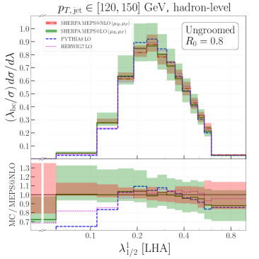
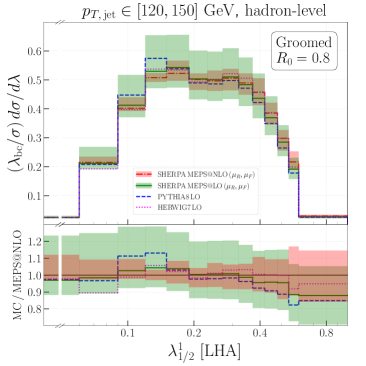
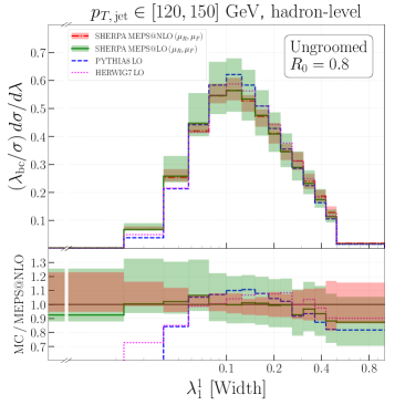
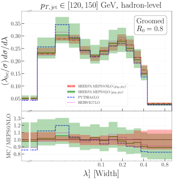
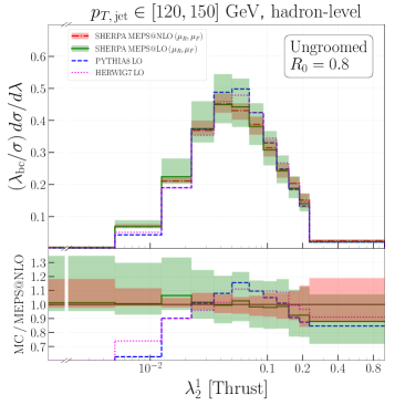
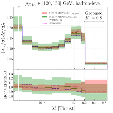
Figure 1: Comparison of hadron-level predictions for ungroomed and groomed jet-angularities in $Zj$ production from P YTHIA and H ERWIG (both based on the LO $Zj$ matrix element), and MEPS@LO as well as MEPS@NLO results from S HERPA . Here $p_{T,\text{jet}}\in[120,150]\;\text{GeV}$ and $\lambda_{\text{bc}}$ stands for the bin centre.

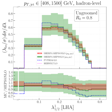
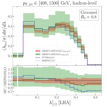
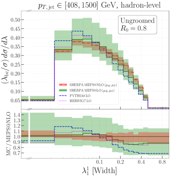
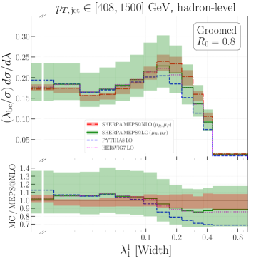
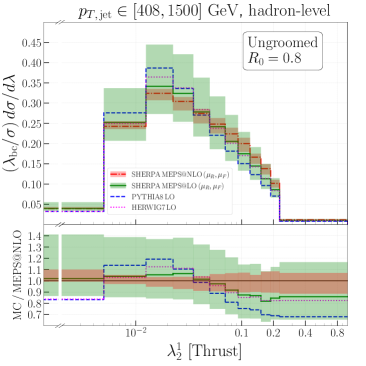
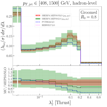
Figure 2: Comparison of hadron-level predictions for ungroomed and groomed jet-angularities in $Zj$ production from P YTHIA and H ERWIG (both based on the LO $Zj$ matrix element), and MEPS@LO as well as MEPS@NLO results from S HERPA . Here $p_{T,\text{jet}}\in[408,1500]\;\text{GeV}$ and $\lambda_{\text{bc}}$ stands for the bin centre.

4 All-order resummation at next-to-leading logarithmic accuracy

To perform the NLL resummation of the jet angularities we use the S HERPA implementation of the C AESAR resummation formalism (Banfi:2004yd, ), first presented in (Gerwick:2014gya, ). This framework has recently been employed to obtain resummed predictions for SoftDrop thrust (Marzani:2019evv, ) and multijet resolution scales (Baberuxki:2019ifp, ) in electron–positron collisions, as well as $\text{NLO}+\text{NLL}^{\prime}$ predictions for SoftDrop groomed hadronic event shapes, in particular groomed transverse thrust (Baron:2020xoi, ).

For a generic observable, the master formula for the all-order cumulative cross section for observable values up to $v$, with $L=-\ln(v)$, can be written as a sum over partonic channels $\delta$:

$$\begin{split}\Sigma_{\mathrm{res}}(v)&=\sum_{\delta}\Sigma_{\mathrm{res}}^{\delta}(v)\,,\,\,\text{with}\\ \Sigma_{\mathrm{res}}^{\delta}(v)&=\int d\mathcal{B_{\delta}}\frac{\mathop{d\sigma_{\delta}}}{\mathop{d\mathcal{B_{\delta}}}}\exp\mathopen{}\mathclose{{}\left[-\sum_{l\in\delta}R_{l}^{\mathcal{B_{\delta}}}(L)}\right]\mathcal{P}^{\mathcal{B}_{\delta}}(L)\mathcal{S}^{\mathcal{B_{\delta}}}(L)\mathcal{F}^{\mathcal{B_{\delta}}}(L)\mathcal{H}^{\delta}(\mathcal{B_{\delta}})\,,\end{split}$$ (11)

where $\frac{\mathop{d\sigma_{\delta}}}{\mathop{d\mathcal{B_{\delta}}}}$ is the fully differential Born cross section for the partonic channel $\delta$ and $\mathcal{H}$ implements the kinematic cuts applied to the Born phase space $\mathcal{B}$. $\mathcal{F}$ denotes the multiple emission function which, for additive observables such as the angularities considered in this paper, is simply given by $\mathcal{F}(L)=e^{-\gamma_{E}R^{\prime}}/\Gamma(1+R^{\prime})$, with $R^{\prime}(L)=\partial R/\partial L$ and $R(L)=\sum_{l\in\delta}R_{l}(L)$. The ratio of parton-distribution-functions (PDFs) $\mathcal{P}$ takes into account the true initial-state collinear scale. The soft function $\mathcal{S}$ implements the non-trivial aspects of colour evolution. The collinear radiators $R_{l}$ for the hard legs $l$ were computed in (Banfi:2004yd, ) for a general observable $V$ scaling for the emission of a soft-gluon of relative transverse momentum $k_{t}^{(l)}$ and relative rapidity $\eta^{(l)}$ with respect to leg $l$ as

$$V(k)=\mathopen{}\mathclose{{}\left(\frac{k_{t}^{\mathopen{}\mathclose{{}\left(l}\right)}}{\mu_{Q}}}\right)^{a}e^{-b_{l}\eta^{\mathopen{}\mathclose{{}\left(l}\right)}}d_{l}\mathopen{}\mathclose{{}\left(\mu_{Q}}\right)g_{l}\mathopen{}\mathclose{{}\left(\phi}\right)\,.$$ (12)

The C AESAR resummation plugin to S HERPA hooks into the event generation framework, facilitating the process management, and providing access to the C OMIX matrix-element generator (Gleisberg:2008fv, ), as well as phase-space integration and event-analysis functionalities. The S HERPA framework is also used to compile all the required higher-order tree-level and one-loop calculations. For the NLO QCD computations we use the S HERPA implementation of the Catani–Seymour dipole subtraction (Gleisberg:2007md, ) and the interfaces to the R ECOLA  (Actis:2016mpe, ; Biedermann:2017yoi, ) and O PEN L OOPS  (Cascioli:2011va, ) one-loop amplitude generators. The plugin implements the building blocks of the C AESAR master formula Eq. (11), along with the necessary expansion in $\alpha_{s}$ used in the matching with fixed-order calculations. The building blocks are evaluated fully differentially for each Born-level configuration $\mathcal{B}_{\delta}$ of a given flavour and momentum configuration.

In Ref. (Baron:2020xoi, ) the C AESAR formalism and the corresponding implementation in the S HERPA plugin were extended to include the phase-space constraints given by SoftDrop grooming with general parameters $z_{\text{cut}}$ and $\beta$. Note that, as already pointed out in (Larkoski:2014wba, ), differential distributions computed from Eq. (11) at NLL are discontinuous at $L=L_{z}=-\ln z_{\text{cut}}$. A way to cure this behaviour was proposed in Ref. (Marzani:2019evv, ). However, as this discontinuity is a subleading (NNLL) effect, we decided to leave it untouched and checked that the two approaches were in agreement within our theoretical uncertainties. Furthermore, we note that our resummation is strictly valid in the limit of small $z_{\text{cut}}$, i.e. $\lambda_{\alpha}\ll z_{\text{cut}}\ll 1$. However, for $\beta=0$ SoftDrop , finite-$z_{\text{cut}}$ corrections are already present at the (leading) single-logarithmic accuracy Dasgupta:2013ihk . For the specific choice of $z_{\text{cut}}=0.1$ adopted in this paper, these corrections have been studied in Marzani:2017mva in the context of the groomed jet mass in dijet processes, and found to have a negligible effect around one percent.

The treatment of the kinematic endpoint is implemented in the same way as in Ref. (Baron:2020xoi, ) by shifting the relevant logarithms and adding power-suppressed terms to achieve a cumulative distribution that approaches one at the kinematic endpoint and has a smooth derivative approaching zero. In particular, we introduce the additional parameters $p,x_{L},v_{\mathrm{max}}$ and modify all logarithms by power-suppressed terms according to

$$\ln\mathopen{}\mathclose{{}\left(\frac{x_{L}}{v}}\right)\to\frac{1}{p}\ln\mathopen{}\mathclose{{}\left[\mathopen{}\mathclose{{}\left(\frac{x_{L}}{v}}\right)^{p}-\mathopen{}\mathclose{{}\left(\frac{x_{L}}{v_{\mathrm{max}}}}\right)^{p}+1}\right]=L\,.$$ (13)

Here we set $v_{\mathrm{max}}$ to the numerically determined endpoint of the NLO distribution, and by default use $p=1$.

We fix the renormalisation and factorisation scale to the transverse momentum of the Z boson, $p_{T,\mu^{+}\mu^{-}}$, and the resummation scale to $\mu_{Q}=p_{T,\mu^{+}\mu^{-}}R_{0}$. Note, for the Born configuration, on which the resummation is performed, it holds $p_{T,\mu^{+}\mu^{-}}\equiv p_{T,\text{jet}}$. To evaluate the perturbative uncertainties of our results, we vary $\mu_{R}$ and $\mu_{F}$ according to a 7-point variation, i.e. $(\mu_{R}/p_{T,\mu^{+}\mu^{-}},\mu_{F}/p_{T,\mu^{+}\mu^{-}})\in\{(0.5,0.5),(0.5,1),(1,0.5),(1,1),(1,2),(2,1),(2,2)\}$, simultaneously in the fixed-order calculation and the resummation. The argument of $\alpha_{\text{s}}$ in the resummation is always taken to be $\mu_{R}$, with a compensating term for the LL dependence to remain NLL accurate and ignoring the NNLL ambiguity this introduces in pure NLL terms. Additionally, we calculate the resummed distribution with $x_{L}\in\{0.5,1,2\}$ for $\mu_{R}=\mu_{F}=p_{T,\mu^{+}\mu^{-}}$. The total uncertainty is obtained by taking the envelope of all those predictions with $(\mu_{R}/p_{T,\mu^{+}\mu^{-}},\mu_{F}/p_{T,\mu^{+}\mu^{-}},x_{L})=(1,1,1)$ as central value.

The ingredients of the master formula Eq. (11) are readily available in the case of global event shapes, with or without SoftDrop grooming. However, some adaptations are needed if we want to apply this approach to the resummation of non-global jet angularity distributions measured on the leading jet in $Z$+jet events. These are described in Section 4.1 below. We then discuss aspects related to the matching to NLO fixed-order calculations in Section 4.2 and present numerical results in Section 4.3.

4.1 Jet angularities resummation within the S HERPA framework

Compared to the formalism described above and used in (Gerwick:2014gya, ; Baberuxki:2019ifp, ; Baron:2020xoi, ), some adjustments are necessary to the S HERPA resummation framework. In particular we have to take into account the fact that the angularities are sensitive to radiation within the hardest jet in the event only. Let us label, for definiteness, the initial state legs as $l=1,2$ and the measured final state leg as $l=3$. As our observable is not sensitive to radiation collinear to the initial state legs, we are allowed to set $\mathcal{P}=1$ and $R_{1}=R_{2}=0$ in Eq. (11). Keeping in mind that the Born phase space is given by final states consisting of a single parton plus the $Z$ boson, only one radiator is left. In terms of Eq. (12), the angularity observables $\lambda^{1}_{\alpha}$ can be parametrised by

$$a =1\,,$$ (14)

$$b_{3} =\alpha-1\,,$$ (15)

$$g_{3}d_{3}(\mu_{Q}) =\mathopen{}\mathclose{{}\left(2\frac{\cosh(y_{3})}{R_{0}}}\right)^{\alpha-1}\frac{\mu_{Q}}{p_{T,\text{jet}}R_{0}}\,,$$ (16)

where $y_{3}\equiv y_{\text{jet}}$ denotes the rapidity of the hard jet. Note that for our choice of $\mu_{Q}=p_{T,\text{jet}}R_{0}$ the last factor in $g_{3}d_{3}$ equals unity.

A number of complications arises when considering the presence of a jet boundary. First, when originally computing the radiators, one conventionally divides the phase space for each dipole at $\eta=0$. An arbitrary rapidity condition with respect to leg $l$, $\eta_{l}>\eta_{\text{min},l}$, leads to an additional contribution

$$\Delta R_{l}(L)=-2C_{l}\mathopen{}\mathclose{{}\left(\eta_{\text{min},l}-\ln 2E_{l}/Q}\right)t(L/a)\,,$$ (17)

where we have introduced

$$t(L)=\int^{\mu_{Q}}_{\mu_{Q}e^{-L}}\frac{dk_{t}}{k_{t}}\frac{\alpha_{\text{s}}\mathopen{}\mathclose{{}\left(k_{t}}\right)}{\pi}=\frac{-\ln(1-2\alpha_{s}\beta_{0}L)}{2\pi\beta_{0}}\,,$$ (18)

with $\beta_{0}=(11C_{A}-2n_{f})/(12\pi)$. Note that the last equality holds with $\alpha_{\text{s}}=\alpha_{\text{s}}(\mu_{R})$ at NLL accuracy. We can use this to reflect the rapidity requirement given by the jet condition by setting $\eta_{\text{min},3}=\ln\mathopen{}\mathclose{{}\left(2\cosh(y_{3})/R_{0}}\right)$. Here $Q$ is an arbitrary scale, which we choose to identify with the partonic centre-of-mass energy, that ultimately cancels in the final expressions. For global observables this cancellation happens with the soft function $\mathcal{S}$, however, the restriction to radiation inside the jet additionally affects the structure of soft emissions. The details were worked out in (Dasgupta:2012hg, ) for the jet-mass observable. Those results apply to the general class of angularities as well, as they depend on the scaling of the observable with $k_{t}$ only, i.e. on the parameter $a$ in Eq. (12). This implies (using $a=1$)

$$\mathcal{S}^{\mathcal{B}_{\delta}}(L)=S_{\text{global}}^{\mathcal{B}_{\delta}}\mathopen{}\mathclose{{}\left(t(L)}\right)S_{\text{non-global}}^{\mathcal{B}_{\delta}}\mathopen{}\mathclose{{}\left(t(L)}\right)\;.$$ (19)

In a general way, the global contribution can be written as

$$S_{\text{global}}^{\mathcal{B}_{\delta}}(t)=\operatorname{Tr}\mathopen{}\mathclose{{}\left[He^{-t\mathopen{}\mathclose{{}\left(\mathbf{\Gamma}^{\mathcal{B}_{\delta}}}\right)^{\dagger}}ce^{-t\mathbf{\Gamma}^{\mathcal{B}_{\delta}}}}\right]/\operatorname{Tr}\mathopen{}\mathclose{{}\left[cH}\right]\;,$$ (20)

where $c$ and $H$ are the colour metric and hard function, respectively, see (Gerwick:2014gya, ; Baberuxki:2019ifp, ) for details of the notation. We can write the matrix $\mathbf{\Gamma}$ in colour space as a sum over dipoles

$$\mathbf{\Gamma}^{\mathcal{B}_{\delta}} =\sum_{i>j\in\mathcal{B}_{\delta}}\mathbf{T}_{i}\cdot\mathbf{T}_{j}I_{ij}\,.$$ (21)

In our case only three dipoles, namely 12, 13 and 23, contribute to the soft function. As a consequence, by exploiting colour conservation, all colour operators $\mathbf{T}_{i}\cdot\mathbf{T}_{j}$ can be written as linear combinations of the $SU(3)$ Casimir invariants $C_{F}$ and $C_{A}$ and, consequently, the matrix structure of Eq. (20) disappears. The coefficients of the single-logarithmic function $t$, can be obtained by integrating the matrix elements for each dipole $ij$ over the appropriate phase space. Because the collinear contributions have already been included in the radiators $R_{l}$ in Eq. (11), the $I_{ij}$ coefficients are purely due to soft wide-angle radiation. Consequently, they are functions of the jet radius $R_{0}$ only, and are independent of the angularity exponent $\alpha$. In particular, they coincide with those computed in (Dasgupta:2012hg, ) for the jet mass:

$$I_{12} =\frac{R^{2}_{0}}{4}\,,$$ (22)

$$I_{13}=I_{23} =\frac{R^{2}_{0}}{16}+\mathcal{O}(R^{4}_{0})\,.$$ (23)

Note that by including the above dipoles we account for initial-state radiation at NLL accuracy, as an expansion in powers of the jet radius. Higher order terms in the jet radius expansion can be computed, but in addition to the suppression in $R^{2}_{0}$ the corresponding coefficient drops rapidly, and even for $R_{0}=1$ the first terms are an appropriate approximation (Dasgupta:2012hg, ).

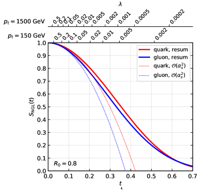
Figure 3: Sudakov suppression factor associated with the non-global logarithms, $S_{\text{non-global}}^{(3)}\mathopen{}\mathclose{{}\left(t(L)}\right)$. The two curves correspond to the case where the final-state parton is either a quark (solid red) or a gluon (dashed blue). The Sudakov is plotted as a function of the scaled variable $t(L)$ (cf. Eq. (18)). For illustrative purpose, the top axes show the corresponding values of $\lambda_{\alpha}^{1}$ (irrespective of $\alpha$) for two representative jet transverse momenta.

The non-global part $S_{\text{non-global}}^{\mathcal{B}_{\delta}}(t)$ is computed numerically, in the large-$N_{c}$ limit, following the algorithm highlighted in (Dasgupta:2001sh, ), as also done in (Dasgupta:2012hg, ). This can straightforwardly be applied to ungroomed angularities. For SoftDrop groomed distributions, the non-global factor remains the same for $v\geq z_{\text{cut}}$ and saturates at that value, i.e. $S_{\text{non-global}}^{\text{(groomed)}}(v)=S_{\text{non-global}}^{\text{(ungroomed)}}(\text{max}(v,z_{\text{cut}}))$. We also note that the non-global contribution only depends on $v$ (and the jet transverse momentum through $\alpha_{s}(\mu_{R})$) but not on the angularity parameter $\alpha$. Similarly, for the groomed case, the contribution from non-global logarithms only depends on $z_{\text{cut}}$ and not on $\beta$. The main reason behind this is that, at single-logarithmic accuracy, non-global logarithms originate from configurations that are strongly ordered in energy with angles commensurate with the jet radius $R_{0}$.

In practice, $S_{\text{non-global}}(t)$ is computed separately for each possible colour dipole, either incoming–incoming or incoming–final. These contributions are independent of the jet rapidity meaning, in particular, that the two possible incoming–final configurations are equal. One can then reconstruct the two Born channels $\delta$ from the dipole contributions as done in (Dasgupta:2012hg, ). This procedure allows one to recover the full-$N_{c}$ result at least for the first non-trivial term of the expansion in $\alpha_{s}$. We finally note that the numerical procedure described in (Dasgupta:2001sh, ) introduces an angular cut-off $\theta_{\text{min}}$ to regulate the collinear divergence. We have performed 4 independent runs with $\theta_{\text{min}}=\{0.008,0.004,0.002,0.001\}$ and extrapolated the result to $\theta_{\text{min}}\to 0$ using the same approach as in (Dasgupta:2020fwr, ).

Fig. 3 shows the resulting non-global contributions $S_{\text{non-global}}^{\mathcal{B}_{\delta}}(t)$ for both (Born-level) quark and gluon jets. The upper set of axes indicate what value of $t$ corresponds to the observable value $\lambda^{1}_{\alpha}$ for fixed $p_{T,\text{jet}}$. We have checked that they agree within $\sim 1\%$ with the results obtained in (Dasgupta:2012hg, ) at $t\lesssim 0.4$. However, the results presented here extend to larger values of $t$, as appropriate for the kinematic range investigated in this paper.

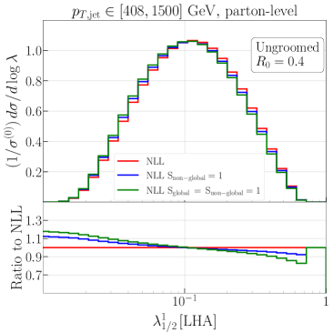
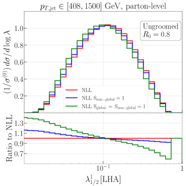
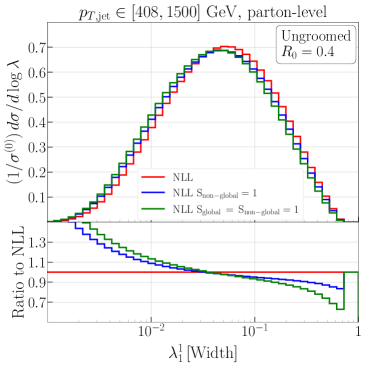
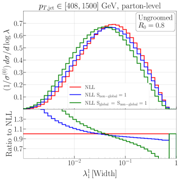
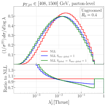
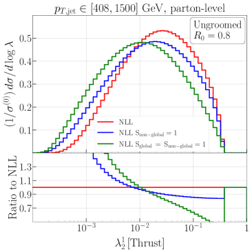
Figure 4: Anatomy of soft structure of the NLL predictions for angularities $\lambda^{1}_{\alpha}$, for $\alpha\in\{1/2,1,2\}$ (top to bottom), for jet radius $R_{0}=0.4$ (left) and $R_{0}=0.8$ (right), with $p_{T,\text{jet}}\in[408,1500]~{}\text{GeV}$. Besides the full NLL distribution (red) variants obtained by either excluding the non-global soft contribution ($S_{\text{non-global}}=1$, blue) or the entire soft contributions ($S_{\text{global}}=S_{\text{non-global}}=1$, green) are shown.

To gauge the numerical impact of the global and non-global soft function on our NLL predictions for the jet-angularity variables, we present in Fig. 4 results for the ungroomed case. As both $\mathcal{S}$-function contributions contain terms expected to vanish in the $R_{0}\to 0$ limit, we here show results for the two considered jet radii, $R_{0}=0.4$ and $R_{0}=0.8$. Besides the complete NLL distribution (in red), we depict results for $S_{\text{non-global}}=1$ (in blue), allowing us to quantify the numerical effect of non-global logarithms, and $S_{\text{global}}=S_{\text{non-global}}=1$ (in green), effectively neglecting soft wide-angle emissions entirely. We observe that these contributions have a bigger impact for larger jet radii as theoretically anticipated. Furthermore, we observe a somewhat milder (relative) impact of $\mathcal{S}$ in the $\alpha=0.5$ case, when comparing to $\alpha=2$. For the latter a quite significant shift of the distribution is found. The case $\alpha=1$ lies in between the other two. This is understood from the fact that, for a given value of the angularity, the soft function is independent of $\alpha$ while the effect of the collinear contribution increases when decreasing $\alpha$. When invoking grooming, the soft function remains unchanged for observable values larger than the transition point. However, below the transition point the soft-function contributions become constant, given by $S_{\text{non-global}}(z_{\text{cut}})$ and $S_{\text{non-global}}(z_{\text{cut}})S_{\text{global}}(z_{\text{cut}})$, respectively. This is illustrated and confirmed in Fig. 15 in App. A.1. We have checked explicitly that our observations on the impact of the soft function both for the groomed and ungroomed case also hold after matching to NLO, as described in what follows.

We close this discussion of the NLL resummation, by noting, had we defined jets with algorithms that differ from anti-$k_{t}$, for instance, C/A or $k_{t}$, a new class of so-called clustering logarithms would have appeared at NLL, see e.g. (Banfi:2005gj, ; Delenda:2006nf, ; Banfi:2010pa, ; Delenda:2012mm, ; Lifson:2020gua, ).

4.2 Matching to NLO and achieving $\text{NLL}^{\prime}$ accuracy

In order to achieve a faithful description of the angularity distributions across their whole spectrum, we need to match our all-order results with fixed-order predictions, computed here at NLO accuracy. Our matching procedure will keep track of the jet flavour, so that we can obtain what is usually referred to as $\text{NLO}+\text{NLL}^{\prime}$ accuracy.

The matching procedure is defined for the cumulative distribution (for simplicity, we use $\lambda\equiv\lambda_{\alpha}^{1}$)

$$\Sigma(\lambda)=\int_{0}^{\lambda}\mathop{d\sigma}.$$ (24)

We also introduce the notation $\Sigma^{\delta}_{\mathrm{res,fo,match}}$ (see also (Baberuxki:2019ifp, ; Baron:2020xoi, )) in order to denote the results for the cumulative distribution for the (family of) flavour channel(s) $\delta$ computed, with resummation, at fixed order, or matched between the two, respectively. In the following, the channel label is omitted in general expressions and we use the shorthand $\sigma=\Sigma(1)$. We denote the expansion of any cumulative distribution $\Sigma$ to order $\alpha_{s}^{2}$ relative to the $pp\to\mu^{+}\mu^{-}j$ Born process as

$$\Sigma=\Sigma^{(0)}+\Sigma^{(1)}+\Sigma^{(2)}+{\cal{O}}(\alpha_{s}^{4})\,,\hskip 28.45274pt\Sigma^{(k)}\propto\alpha^{2}_{\text{EW}}\,\alpha_{s}^{1+k}\,.$$ (25)

In practice, at least for $\Sigma^{(2)}_{\mathrm{fo}}$, we only calculate

$$\overline{\Sigma}^{(2)}_{\mathrm{fo}}(\lambda)=\int_{\lambda}^{1}\mathop{d\sigma^{(2)}}~{},\hskip 28.45274pt\Sigma^{(2)}_{\mathrm{fo}}=\sigma^{(2)}_{\mathrm{fo}}-\overline{\Sigma}^{(2)}_{\mathrm{fo}}\,.$$ (26)

We employ a multiplicative matching scheme, in which, for every partonic channel $\delta$, we have

$$\Sigma_{\text{match,mult}}^{\delta}(\lambda)=\Sigma_{\text{res}}^{\delta}(\lambda)\mathopen{}\mathclose{{}\left[1+\frac{\Sigma_{\mathrm{fo}}^{\delta,(1)}(\lambda)-\Sigma_{\mathrm{res}}^{\delta,(1)}(\lambda)}{\sigma^{\delta,(0)}}}\right.\\ \mathopen{}\mathclose{{}\left.+\frac{1}{\sigma^{\delta,(0)}}\mathopen{}\mathclose{{}\left(-\overline{\Sigma}^{\delta,(2)}_{\mathrm{fo}}(\lambda)-\Sigma_{\mathrm{res}}^{\delta,(2)}(\lambda)-\Sigma_{\mathrm{res}}^{\delta,(1)}(\lambda)\frac{\Sigma_{\mathrm{fo}}^{\delta,(1)}(\lambda)-\Sigma_{\mathrm{res}}^{\delta,(1)}(\lambda)}{\sigma^{\delta,(0)}}}\right)}\right]\;.$$ (27)

By this procedure we automatically include the correct coefficients

$$\frac{\alpha_{s}}{2\pi}C^{\delta,(1)}\equiv\lim\limits_{\lambda\to 0}\frac{\Sigma_{\mathrm{fo}}^{\delta,(1)}(\lambda)-\Sigma_{\mathrm{res}}^{\delta,(1)}(\lambda)}{\sigma^{\delta,(0)}}\,,$$ (28)

thus reaching $\text{NLO}+\text{NLL}^{\prime}$ accuracy. The final result we present corresponds to

$$\Sigma_{\text{match,mult}}(\lambda)=\sum_{\delta}\Sigma_{\text{match,mult}}^{\delta}(\lambda)\,.$$ (29)

We use the anti-$k_{t}$ algorithm with our choice of parameters for defining jets, and employ the flavour-$k_{t}$ algorithm from (Banfi:2006hf, ) (BSZ) to assign the flavour channels. However, the BSZ algorithm is not immediately applicable here, due to the non-global structure of the angularities. In particular, at any perturbative order there exist contributions with only a single jet constituent, such that the angularity variable equals zero. In principle we need to perform the resummation around multi-jet configurations. However, to achieve our target accuracy, it is sufficient to guarantee that configurations occuring at LO are dressed with the proper LL Sudakov factor. An explicit example is given in Fig. 5(b). Our matching scheme achieves this by multiplying these $Z+jj$ events with the full NLL $\Sigma^{\delta}_{\text{res}}$ corresponding to the channel $\delta$ obtained after dropping the second jet, which will contain the correct LL factor. It is hence crucial that the flavour channel of those contributions is defined by the single object inside the leading jet alone. At the same time, in the example shown in Fig. 5(a), the quarks need to be clustered in the collinear limit and the jet identified as a gluon jet. While at this stage we could just use the combined flavour of all anti-$k_{t}$ jet constituents, NLO contributions would spoil the IR safety of this procedure. Examples of relevant configurations are given in Fig. 5(c) and (d), where an IR-safe algorithm needs to ensure that the $g\to q\bar{q}$ splitting is undone first in the soft gluon limit. Here we propose and employ the following algorithm to assign flavour to the leading anti-$k_{t}$ jet:

1. Start with the list $\mathcal{O}$ of all coloured final-state objects, containing particle four-momenta and flavour labels, and the beams $B,\bar{B}$ with their respective flavours.

2. Run the standard anti-$k_{t}$ algorithm with radius parameter $R_{0}$ on $\mathcal{O}$, and obtain the objects in the leading, i.e. highest $p_{T}$, jet $J\subset\mathcal{O}$.

3. If $J$ consists of only one object, $J=\{j\in\mathcal{O}\}$, terminate the algorithm. The flavour of $j$ defines the flavour channel $\delta$.

4. Otherwise, determine the pair $\{i,k\}\subset\mathcal{O}$ that minimises the BSZ measure $d_{ik}^{\text{BSZ}}$ and the objects $l,m$ that have minimal BSZ distances to the beams $d_{lB}^{\text{BSZ}},d_{m\bar{B}}^{\text{BSZ}}$. Perform a cluster step according to $d^{\text{BSZ}}=\min(d_{ik}^{\text{BSZ}},d_{lB}^{\text{BSZ}},d_{m\bar{B}}^{\text{BSZ}})$:

   1. If $d^{\text{BSZ}}=d_{ik}^{\text{BSZ}}$, update $\mathcal{O}$ by removing $i$ and $k$ and adding a new object with momentum $p_{i}+p_{k}$ and the combined flavour of objects $i$ and $k$.

   2. If $d^{\text{BSZ}}=d_{lB}^{\text{BSZ}}$ ($d^{\text{BSZ}}=d_{m\bar{B}}^{\text{BSZ}}$), update $\mathcal{O}$ by removing $l$ ($m$) and assign the combined flavour of $l$ and $B$ ($m$ and $\bar{B}$) to the beam $B$ ($\bar{B}$).

   Go to step 1 and repeat.

We finally can define bland versions of this algorithm, vetoing clusterings that would lead to jets with multiple flavours by setting the corresponding distance measures to infinity. We use this bland variant and identify every event as having a leading jet that is either quark- or gluon-like.

(a)                           (b)                             (c)                             (d)

Figure 5: Examples for partonic input configurations to the flavour assignment algorithm. Configuration (a) needs to be identified as a gluon jet in the collinear limit, whereas for (b) we need to perform the LL resummation for a quark jet. IR safety requires that configurations (c) and (d) in the limit where $p_{g}\to 0$ are identified as gluon and quark jet, respectively.

Note that the only contribution that matters are the cross terms between $C^{\delta,(1)}$ and the leading logarithms, which only depend on this flavour assignment and not on details of partons outside the jet. Therefore, we can sort any configuration with the same flavour assignment of the leading jet into the same channel. With this procedure we can ensure a correct assignment of the LO real corrections, while maintaining an infrared-safe definition of jet flavour also at NLO.

4.3 $\text{NLO}+\text{NLL}^{\prime}$ validation and predictions

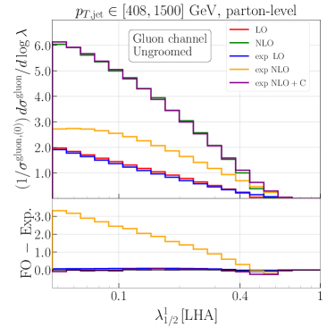
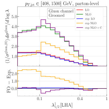
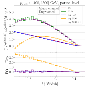
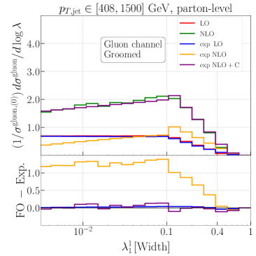
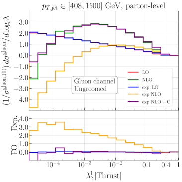
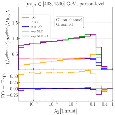
Figure 6: Fixed-order predictions for the gluon channel, identified with the BSZ algorithm, for ungroomed (left column) and groomed (right column) angularities $\lambda^{1}_{\alpha}$, for $\alpha\in\{1/2,1,2\}$, compared to the expansion of the resummation at the corresponding order of $\alpha_{\text{s}}$, see text for details. The jet transverse momentum is constrained to $p_{T,\text{jet}}\in[408,1500]~{}\text{GeV}$.

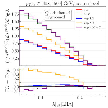
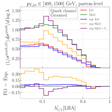
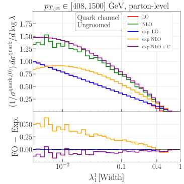
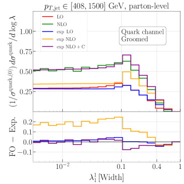
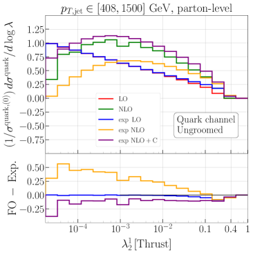
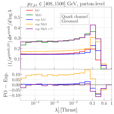
Figure 7: Fixed-order predictions for the quark channel, identified with the BSZ algorithm, for ungroomed (left column) and groomed (right column) angularities $\lambda^{1}_{\alpha}$, for $\alpha\in\{1/2,1,2\}$, compared to the expansion of the resummation at the corresponding order of $\alpha_{\text{s}}$, see text for details. The jet transverse momentum is constrained to $p_{T,\text{jet}}\in[408,1500]~{}\text{GeV}$.

Splitting up the full fixed-order calculation into separate flavour channels in an infrared safe way, enables us to validate our results, in particular the effective inclusion of the $C^{\delta,(1)}$ coefficients, for each partonic channel $\delta$ individually. We hence compare the leading-order contributions

$$\Sigma_{\text{LO}}^{\delta}(\lambda) =\sigma^{\delta,(0)}+\Sigma_{\mathrm{fo}}^{\delta,(1)}(\lambda)\,,$$ (30)

$$\Sigma_{\text{exp LO}}^{\delta}(\lambda) =\sigma^{\delta,(0)}+\Sigma_{\mathrm{res}}^{\delta,(1)}(\lambda)\,,$$ (31)

obtained respectively for the exact matrix element and for the expansion of the resummed calculation. Similarly, at NLO, we compare

$$\Sigma_{\text{NLO}}^{\delta}(\lambda) =\sigma^{\delta,(0)}+\Sigma_{\mathrm{fo}}^{\delta,(1)}(\lambda)-\overline{\Sigma}^{\delta,(2)}_{\mathrm{fo}}(\lambda)\,,$$ (32)

$$\Sigma_{\text{exp NLO}}^{\delta}(\lambda) =\sigma^{\delta,(0)}+\Sigma_{\mathrm{res}}^{\delta,(1)}(\lambda)+\Sigma^{\delta,(2)}_{\mathrm{res}}(\lambda)\,,$$ (33)

$$\Sigma_{\text{exp NLO+C}}^{\delta}(\lambda) =\sigma^{\delta,(0)}+\mathopen{}\mathclose{{}\left(1+\frac{\Sigma_{\mathrm{fo}}^{\delta,(1)}(\lambda)-\Sigma_{\mathrm{res}}^{\delta,(1)}(\lambda)}{\sigma^{\delta,(0)}}}\right)\Sigma_{\mathrm{res}}^{\delta,(1)}(\lambda)+\Sigma^{\delta,(2)}_{\mathrm{res}}\,,$$ (34)

where $\Sigma_{\text{exp NLO}}^{\delta}(\lambda)$ is the NLO expansion of the all-order result, while $\Sigma_{\text{exp NLO+C}}^{\delta}(\lambda)$ also includes the contribution from the $C^{\delta,(1)}$ coefficient. Note that $\Sigma_{\text{NLO}}(1)=\Sigma_{\text{LO}}(1)=\sum_{\delta}\mathopen{}\mathclose{{}\left(\sigma^{\delta,(0)}+\sigma^{\delta,(1)}_{\mathrm{fo}}}\right)$.

In Figs. 6 and 7 we present the differential distributions $d\sigma/d\log\lambda\equiv d\Sigma(\lambda)/d\log\lambda$ in $\lambda$, separately for the gluon (Fig. 6) and quark (Fig. 7) channel, identified by the BSZ flavour-$k_{t}$ algorithm, for the representative jet-$p_{T}$ slice $p_{T,\text{jet}}\in[408,1500]\;\text{GeV}$. We have checked that analogous results are obtained for the other transverse momentum slices. In all these validations we assume a jet radius of $R_{0}=0.8$. As before, we consider the angularities $\lambda^{1}_{\alpha}$ with $\alpha\in\{1/2,1,2\}$ either without grooming or with SoftDrop grooming using $z_{\text{cut}}=0.1,\,\beta=0$. For each observable we include an additional panel that contains the differences between the fixed-order result, i.e. Eqs. (30) and (32), and the expansions of the resummation up to order $\alpha_{\text{s}}$ and $\alpha_{\text{s}}^{2}$, i.e. Eqs. (31) and (33), (34), respectively.

We first note that for all angularities — groomed or ungroomed — the difference between the derivatives of $\Sigma_{\text{LO}}$ and $\Sigma_{\text{exp LO}}$ vanishes for $\lambda\ll 1$, as expected in the ungroomed case. For the groomed angularities there are in principle, for $\beta=0$, deviations of $\mathcal{O}(z_{\text{cut}})$. Those appear to be too small to observe numerically here, as was also observed for example for event shapes in Baron:2020xoi . In comparing $d\Sigma_{\text{NLO}}/dL$ and $d\Sigma_{\text{exp NLO}}/dL$ (with $L\equiv\log(1/\lambda)$) we observe a linearly rising difference, indicating missing terms of order $\alpha_{\text{s}}^{2}L^{2}$ in $\Sigma_{\text{exp NLO}}$. By including the $C^{\delta,(1)}$ coefficient in $\Sigma_{\text{exp NLO+C}}$, the derivatives only differ by a constant, confirming that missing terms in the cumulative distribution are reduced to order $\alpha_{\text{s}}^{2}L$.

Having validated our resummation calculations by comparing their expansions to the corresponding fixed-order predictions, we finally present our matched resummed $\text{NLO}+\text{NLL}^{\prime}$ results and compare them to their NLO counterparts. Figs. 8 and  9 contain our predictions for the two considered transverse-momentum slices, using the same set of observables and grooming parameters as above. These figures also illustrate how the full result is obtained as the sum of the two flavour channels — quarks and gluons — identified by our BSZ flavour-assignment procedure. We note that, for all observables, the contribution from gluon jets is increased for the higher $p_{T,\text{jet}}$ slice compared to the case $p_{T,\text{jet}}\in[120,150]~{}\text{GeV}$. However, for both slices we observe a more significant contribution from gluon jets for larger values of the angularities, while the low-$\lambda^{1}_{\alpha}$ tails are entirely dominated by quark jets. This is a confirmation that a cut on the jet angularity can serve as a theoretically well-defined and IRC safe quark–gluon discriminant, as pointed out, for instance, in Refs. (Gras:2017jty, ; Badger:2016bpw, ; Larkoski:2013eya, ; Larkoski:2014pca, ). We leave further investigation on this topic to future work. In addition to the matched resummation, we show the full fixed-order predictions at NLO accuracy. All-order effects turn out to be important essentially over the entire observable range. In particular, only for the highest values of the observables do NLO and matched predictions start to look similar. This appears to be the case for both ungroomed and groomed distributions. After a detailed analysis, we have concluded that this effect, the size of which is rather surprising, is driven by the large constant contribution of Eq. (28), which in turn originate from the large perturbative corrections that characterise the $Z$+jets process. Similar observations have been reported for the groomed jet mass in $Zj$ production in Ref. (Frye:2016aiz, ).

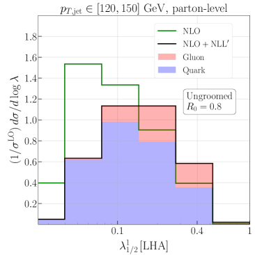
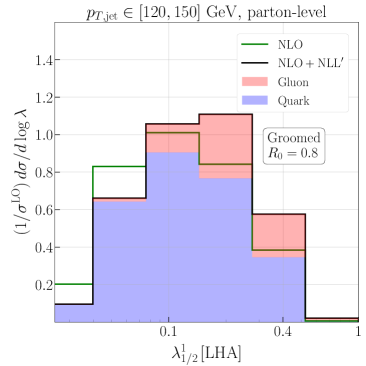
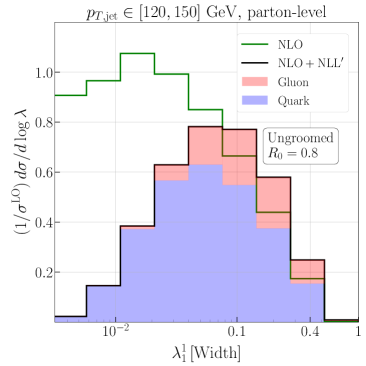
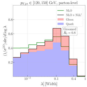
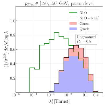
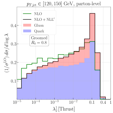
Figure 8: Fixed-order and matched predictions at NLO and $\text{NLO}+\text{NLL}^{\prime}$ accuracy, for ungroomed (left row) and groomed (right row) angularities, for $\alpha\in\{1/2,1,2\}$. The colour scheme indicates how the gluon (red) and quark (blue) channel as identified with the BSZ algorithm stack up to form the $\text{NLO}+\text{NLL}^{\prime}$ prediction. The jet transverse momentum is constrained to $p_{T,\text{jet}}\in[120,150]~{}\text{GeV}$.

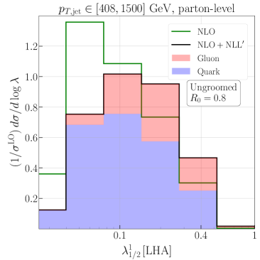
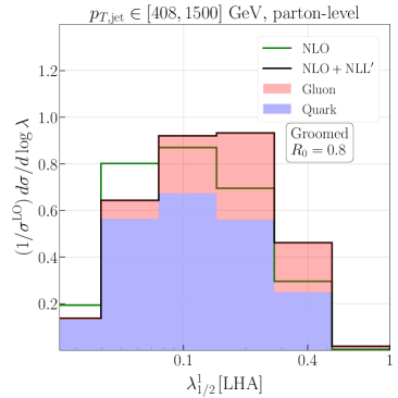
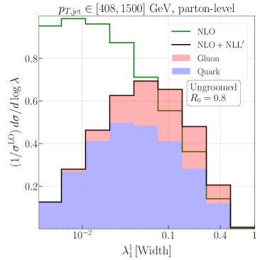
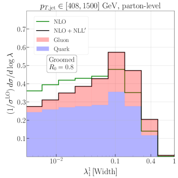
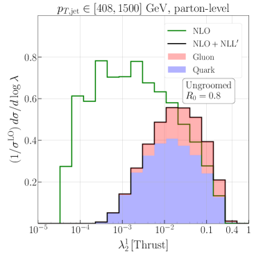
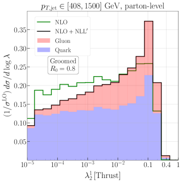
Figure 9: Fixed-order and matched predictions at NLO and $\text{NLO}+\text{NLL}^{\prime}$ accuracy, for ungroomed (left row) and groomed (right row) angularities, for $\alpha\in\{1/2,1,2\}$. The colour scheme indicates how the gluon (red) and quark (blue) channel as identified with the BSZ algorithm stack up to form the $\text{NLO}+\text{NLL}^{\prime}$ prediction. The jet transverse momentum is constrained to $p_{T,\text{jet}}\in[408,1500]~{}\text{GeV}$.

5 Final predictions

In this section we provide our final theoretical predictions for the leading-jet angularities. We start the discussion with a comparison of our $\text{NLO}+\text{NLL}^{\prime}$ results with parton-level MC predictions from the P YTHIA , H ERWIG and S HERPA event generators. We then discuss the size of non-perturbative corrections due to hadronisation and UE, and demonstrate how to account for these effects in our final $\text{NLO}+\text{NLL}^{\prime}$ predictions.

5.1 $\text{NLO}+\text{NLL}^{\prime}$ at parton level

Let us start by comparing our $\text{NLO}+\text{NLL}^{\prime}$ results for the jet angularities against different parton-level MC predictions. As in Section 3 we consider the LHA ($\lambda^{1}_{1/2}$), Width ($\lambda^{1}_{1}$), and Thrust ($\lambda^{1}_{2}$) observables. In Figs. 10 and 11 we compare the $\text{NLO}+\text{NLL}^{\prime}$ distributions against the parton-level MEPS@NLO predictions of S HERPA and the LO results from P YTHIA and H ERWIG . As before we consider two $p_{T,\text{jet}}$ slices, namely $p_{T,\text{jet}}\in[120,150]$ GeV in Fig. 10 and $p_{T,\text{jet}}\in[408,1500]$ GeV in Fig. 11. The theoretical uncertainty for the resummed and matched predictions is obtained by varying renormalisation ($\mu_{R}$) and factorisation ($\mu_{F}$) scales, as well as the parameter $x_{L}$ that determines the resummation scale, as detailed in Sec. 4, while the uncertainty band of the S HERPA MEPS@NLO predictions corresponds to variations of $\mu_{R}$ and $\mu_{F}$ only, however, both in the matrix element and parton-shower component. For this reason, the former yields a more conservative assessment of the uncertainty than the latter.

A useful viewpoint to understand our results is to consider the different types of contributions that affect the distributions. Roughly speaking, even at parton level, the behaviour of the distributions at low values of the observables strongly depends on the details of the treatment of radiation in the infrared region, e.g. the parton-shower cutoff or the Landau pole in the resummation. This region is characterised by large non-perturbative corrections, mostly due to hadronisation. The size of the region depends on the angularity exponent $\alpha$, the presence of grooming and the considered transverse momentum region. Following the analysis of, e.g., Refs. (Dasgupta:2013ihk, ; Larkoski:2014wba, ) we can estimate the region of large non-perturbative corrections to be

ungroomed jets or SoftDrop jets with $$\alpha\leq 1 \quad\lambda^{1}_{\alpha}\lesssim\mathopen{}\mathclose{{}\left(\frac{\mu_{\text{NP}}}{p_{T,\text{jet}}R_{0}}}\right)^{\min(\alpha,1)}\,,$$: (35)

SoftDrop jets with $$\alpha>1 \quad\lambda^{1}_{\alpha}\lesssim\mathopen{}\mathclose{{}\left(\frac{\mu_{\text{NP}}}{p_{T,\text{jet}}R_{0}}}\right)\mathopen{}\mathclose{{}\left(\frac{\mu_{\text{NP}}}{z_{\rm cut}p_{T,\text{jet}}R_{0}}}\right)^{\frac{\alpha-1}{1+\beta}}\,,$$: (36)

where $\mu_{\text{NP}}$ is a non-perturbative scale that we take to be $1$ GeV. For $\alpha\leq 1$, the non-perturbative corrections first come from the region of hard-collinear radiation which is mostly unaffected by the grooming procedure. Conversely, when applying SoftDrop for angularities with $\alpha>1$, the factor in the second bracket of Eq. (36) is smaller than 1 and the boundary of the non-perturbative region is pushed towards smaller observable values. Above the thresholds identified by Eqs. (35), (36), we expect (resummed) perturbation theory to provide a good description of the underlying physical processes. In this second region we can expect our $\text{NLO}+\text{NLL}^{\prime}$ predictions and the MC ones to agree best. Finally, we can identify a third region, which is characterised by very large values of the observables, close to the kinematic endpoint of the distribution. In our resummed and matched prediction this region is under the jurisdiction of the NLO calculation, however the actual value of the kinematic endpoint is strongly affected by the presence of additional emissions, as captured by the parton-shower simulations. For the same reason, we also expect this very last bin to be rather sensitive to non-perturbative contributions, especially the UE, as we shall discuss below.

We can now move to analyse in more detail the various cases. First of all we consider the ungroomed $\lambda^{1}_{1/2}$ distribution for the lower transverse momentum bin in Fig. 10. From the qualitative argument of Eq. (35), we expect the boundary between the first two regions to be located around $\lambda^{1}_{1/2}\simeq 0.1$. Indeed, in the region to the left of this value the agreement between the $\text{NLO}+\text{NLL}^{\prime}$ and the three parton-level MC predictions is rather poor, with the $\text{NLO}+\text{NLL}^{\prime}$ and S HERPA MEPS@NLO uncertainty bands not overlapping. Above this value, the agreement improves, as expected, until we end up in the third region, close to the endpoint, where the predictions from the two approaches are in strong disagreement. The situation does not improve with SoftDrop ​​, as we have anticipated earlier. If anything the agreement between the two predictions deteriorates at the boundary between the first and second region. We attribute this to the presence of transition-point effects (remember that we have chosen $z_{\rm cut}=0.1$). However, as these are formally NNLL effects, they are not very-well modelled by our calculation. In the case of the higher transverse momentum bin, the boundary between the first two regions is pushed to smaller values of the observable ($\lambda^{1}_{1/2}\simeq 0.05$) and, consequently, the region where we find agreement between resummation and MC simulations should widen. This appears clearly in the top-left plot of Fig. 11, which represents the ungroomed case. In fact, the $\text{NLO}+\text{NLL}^{\prime}$ result is in very good agreement with the P YTHIA prediction. Changes in behaviour of the groomed distribution with respect to the lower-$p_{T}$ case are instead minimal. In both cases, we still see large deviations in the endpoint region. Therefore, we must conclude that the distribution of the LHA observable is not well theoretically controlled in our $\text{NLO}+\text{NLL}^{\prime}$ calculation. Since the different parton-shower simulations agree among themselves much better, a more systematic study of the differences with respect to the analytic approach seems well motivated. In this context we note that Ref. Hoeche:2017jsi presented such comparison for the closely related BKS observables Berger:2002ig ; Berger:2003iw and fractional-energy correlations Banfi:2004yd in $e^{+}e^{-}$ collisions, in an approach that could be extended to groomed observables, also in hadronic collision. In any case, as we shall see shortly, the other angularities considered in this study do not suffer from this problem to the same extend.

Now let us examine the remaining two cases, i.e. the $\lambda^{1}_{1}$ and $\lambda^{1}_{2}$ distributions. Similarly to the $\lambda^{1}_{1/2}$ case it is convenient to consider the three different $\lambda$ regions. Let us concentrate on the $p_{T,\text{jet}}\in[120,150]$ GeV slice in Fig. 10 first. We observe differences between our $\text{NLO}+\text{NLL}^{\prime}$ results and MC predictions in the first region for the ungroomed distributions, i.e. $\lambda^{1}_{\alpha}\lesssim 0.01$.

However, we notice that grooming now significantly improves the overall agreement between the different predictions, especially for the $\lambda^{1}_{2}$ case, as expected from Eq. (36). Differences between $\text{NLO}+\text{NLL}^{\prime}$ and the parton-shower simulations in the endpoint region are also seen in this case, but this time all predictions remain consistent within the estimated uncertainties. We also note the abrupt change of behaviour in the SoftDrop distributions around $\lambda^{1}_{\alpha}\simeq z_{\text{cut}}=0.1$, which marks the boundary between the groomed and ungroomed regions. As already explained, this discontinuity is beyond the accuracy of our resummation and it is therefore reassuring that the theoretical uncertainty in this region is rather large. Finally, we note that the overall agreement between our $\text{NLO}+\text{NLL}^{\prime}$ calculation and the parton showers further improves for high transverse momentum jets, evidenced by Fig. 11. Thus, unlike the case of the LHA observable, the $\text{NLO}+\text{NLL}^{\prime}$ predictions for jet width and jet thrust in general agree with the corresponding results from parton-shower simulations. This allows us to conclude that the $\lambda^{1}_{1}$ and $\lambda^{1}_{2}$ distributions are well under theoretical control. It is interesting to point out that, in the context of quark–gluon discrimination, the ATLAS collaboration has also observed Aad:2014gea a worsening of the agreement between the experimental data and Monte Carlo simulations, for smaller values of $\alpha$ although with large uncertainties.

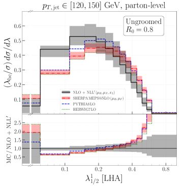
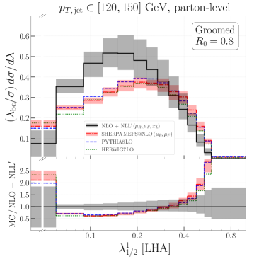
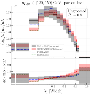
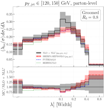
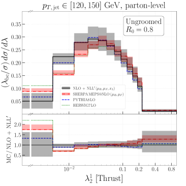
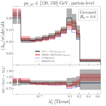
Figure 10: Comparison of parton-level predictions for ungroomed and groomed jet-angularities in $Zj$ production from P YTHIA , H ERWIG (both LO), and S HERPA (MEPS@NLO) with $\text{NLO}+\text{NLL}^{\prime}$ results for $p_{T,\text{jet}}\in[120,150]\;\text{GeV}$. Here $\lambda_{\text{bc}}$ stands for the bin centre.

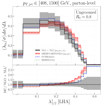
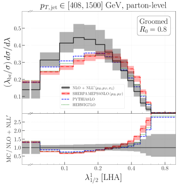
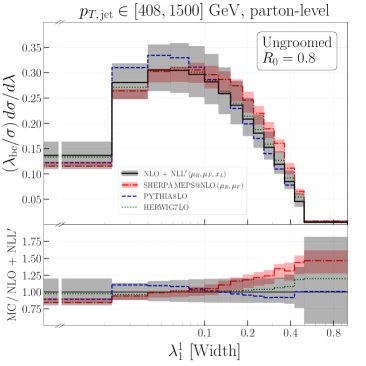
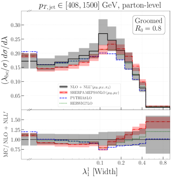
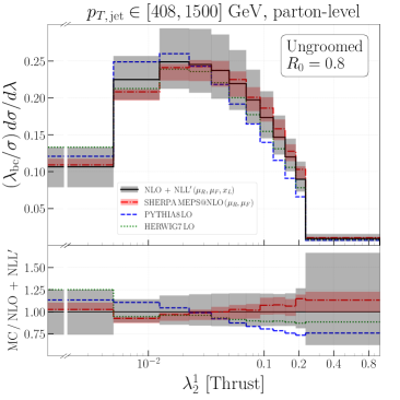
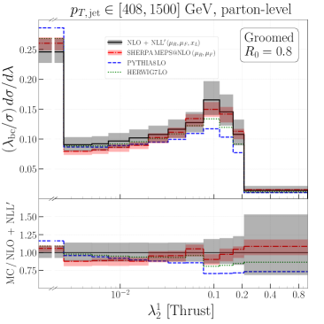
Figure 11: Comparison of parton-level predictions for ungroomed and groomed jet-angularities in $Zj$ production from P YTHIA , H ERWIG (both LO), and S HERPA (MEPS@NLO) with $\text{NLO}+\text{NLL}^{\prime}$ results for $p_{T,\text{jet}}\in[408,1500]\;\text{GeV}$. Here $\lambda_{\text{bc}}$ stands for the bin centre.

5.2 Impact of non-perturbative corrections

Both the $\text{NLO}+\text{NLL}^{\prime}$ and the MC predictions in Section 5.1 were given without including non-perturbative corrections due to the UE and hadronisation. In this section we provide an estimate of these contributions and demonstrate how one can introduce corresponding corrections to our $\text{NLO}+\text{NLL}^{\prime}$ results.

Let us consider the parton-to-hadron transition first. One way to add hadronisation effects to our $\text{NLO}+\text{NLL}^{\prime}$ results is to perform a field-theoretical analysis, based on non-perturbative matrix elements. However, the jet structure may not only be significantly affected by hadronisation but also by the UE. The underlying event, unlike hadronisation, should not be seen as a non-perturbative correction to our $Zj$ matrix elements, but rather as independent semi-hard processes, contributing with additional final-state partons that ultimately hadronise. Therefore, the UE cannot be straightforwardly included into the resummation framework beyond the simple model of uniform radiation (Dasgupta:2007wa, ; Marzani:2017kqd, ). Moreover, hadronisation may lead to non-trivial clustering of partons from different processes, i.e. the hard scattering and the UE, into final-state hadrons. Therefore, we prefer to rely on dynamical non-perturbative models as implemented in the P YTHIA , H ERWIG and S HERPA MC event generators (Buckley:2011ms, ). Each of these programs is using its own default combination of non-perturbative models for hadronisation and UE. More precisely, in both the P YTHIA and S HERPA frameworks the UE is described by the Poisson-based Sjöstrand–Zijl model presented in (Sjostrand:1985vv, ; Sjostrand:1987su, ; Sjostrand:2004pf, ) whereas in H ERWIG the UE is simulated based on the eikonal-model for soft emissions (Bahr:2008dy, ; Gieseke:2016fpz, ). The hadronisation effects are simulated according to the Lund string model (Andersson:1983ia, ; Sjostrand:1984ic, ) in P YTHIA and according to cluster-fragmentation models both in H ERWIG (Webber:1983if, ; Kupco:1998fx, ) and S HERPA (Winter:2003tt, ).

In order to estimate the overall impact of non-perturbative effects we consider the ratios of hadron-to-parton-level predictions. To this end, each MC simulation with P YTHIA , H ERWIG and S HERPA is performed twice: first at parton level (without hadronisation and UE) and second at hadron level (with both UE and hadronisation switched on). This approach allows us to consider the ratio $\mathopen{}\mathclose{{}\left(d\sigma^{\rm HL}/d\lambda}\right)/\mathopen{}\mathclose{{}\left(d\sigma^{\rm PL}/d\lambda}\right)$ evaluated per $\lambda$-bin for each MC generator. The $\mathopen{}\mathclose{{}\left(d\sigma^{\rm HL}/d\lambda}\right)/\mathopen{}\mathclose{{}\left(d\sigma^{\rm PL}/d\lambda}\right)$ ratios obtained with P YTHIA , H ERWIG and S HERPA are then combined into an envelope, with extreme points given by the maximal and minimal predictions per given angularity bin. The central value of the envelope is determined by the respective arithmetic mean value. The resulting ratios, together with their uncertainties are shown in Figs. 12 (a) and (b), differential in $\lambda^{1}_{\alpha}$, for the two representative $p_{T,\text{jet}}$ bins, respectively. Experimental studies of jet structure may be based on all final-state particles, i.e. jet constituents, or purely on the tracks left by charged hadrons only. Therefore, it is convenient to consider two types of $\mathopen{}\mathclose{{}\left(d\sigma^{\rm HL}/d\lambda}\right)/\mathopen{}\mathclose{{}\left(d\sigma^{\rm PL}/d\lambda}\right)$ ratios: the first one where all final-state hadrons in the jet are considered (red solid areas in Fig. 12) and the second one where only the charged jet constituents are used in the evaluation of the angularities (blue hatched areas). We note that the shape and the size of non-perturbative corrections in the two cases are rather similar. By comparing Figs. 12 (a) and (b), we observe that the behaviour of the non-perturbative correction factors obtained here feature all the expected properties. The overall size of the non-perturbative corrections decreases as the transverse momentum increases, in line with our expectation for IRC safe observables. This remains true for the charged-hadrons only case, despite IRC unsafety. Applying SoftDrop typically reduces the size and the onset of non-perturbative corrections, although this feature is less prominent in the LHA case, for which non-perturbative corrections remain rather large also for groomed jets.

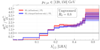
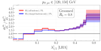
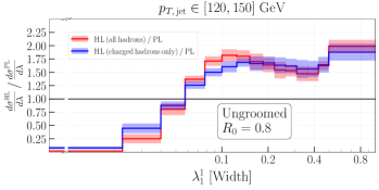
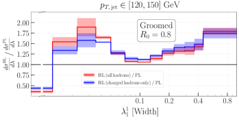
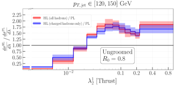
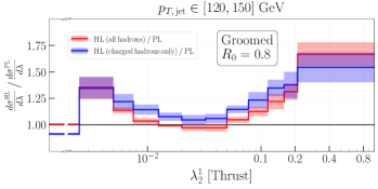
(a)

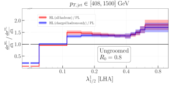
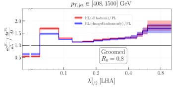
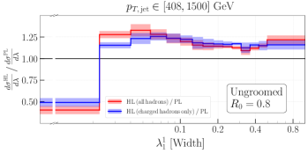
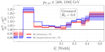
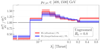
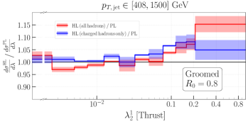
(b)

Figure 12: Hadron-to-parton-level ratios with associated uncertainties extracted from MC simulations. Results are provided for jet angularities based on all hadrons, and charged hadrons only, for $p_{T,\text{jet}}\in[120,150]\;\text{GeV}$ (a) and $p_{T,\text{jet}}\in[408,1500]\;\text{GeV}$ (b).

Finally, we use the results in Fig. 12 to correct our $\text{NLO}+\text{NLL}^{\prime}$ predictions for non-perturbative effects. In order to do that we take our $\text{NLO}+\text{NLL}^{\prime}$ distributions as in Figs. 10 and 11 and multiply them on a per-bin basis by the corresponding central value of the $\mathopen{}\mathclose{{}\left(d\sigma^{\rm HL}/d\lambda}\right)/\mathopen{}\mathclose{{}\left(d\sigma^{\rm PL}/d\lambda}\right)$ ratios shown in Fig. 12. The final uncertainty bands are obtained by summing in quadrature the perturbative and non-perturbative uncertainties.

The $\text{NLO}+\text{NLL}^{\prime}$ + NP distributions, represented by black solid lines, in Figs. 13 and 14 present the main result of this paper. They feature our $\text{NLO}+\text{NLL}^{\prime}$ perturbative predictions and include an MC-based estimate of non-perturbative corrections, here for the case where all hadrons in the jet are considered, for the three angularities $\lambda^{1}_{\alpha}$, for the two representative transverse momentum bins. Corresponding results for the case where only charged tracks are considered in the observable calculation are presented in Appendix A.2 in Figs. 16 and 17. The gray uncertainty bands represent the perturbative, $(\mu_{R},\mu_{F},x_{L})$ variations, and non-perturbative, $\delta_{\text{NP}}$, systematics added in quadrature. For comparison, we also report the S HERPA MEPS@NLO hadron-level predictions, red dashed-dotted lines, including systematic variations of the factorisation and renormalisation scale, red hatched band. We see a good agreement between the two predictions for the jet Width and Thrust. We expect that a comparison to upcoming experimental data would find agreement with these distributions. However, the size of the experimental uncertainties will tell us whether the theoretical calculation needs to be improved, in order to perform precision phenomenology. In this context, these observables could be exploited to extract jet properties, such as the flavour, or, even more ambitiously, parameters of the Standard Model such as couplings and masses. The situation for the LHA distribution is instead in stark contrast. Here the resummed calculation and event-generator predictions are not in agreement, especially in the groomed case. This is true both at parton- and hadron-level. In this case upcoming LHC data may help us to shed light on the discrepancy. The data may favour the MC prediction, indicating that modelling used in the resummed calculation, which for instance neglects recoil, is not appropriate. On the other hand, the data may favour the resummation, indicating the need for a better understanding of the logarithmic structure that is achieved by the parton-shower models.

We conclude this section by reporting that most of the conclusions reached above, also hold for smaller jet radii. Explicit resummed and matched results for $R_{0}=0.4$ , as well as their comparison to S HERPA MEPS@NLO predictions, are collected in Appendix A.3.

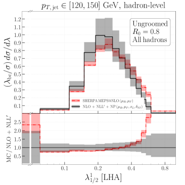
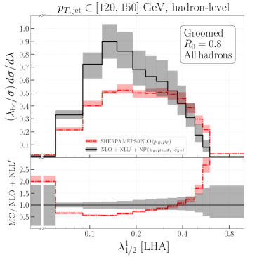
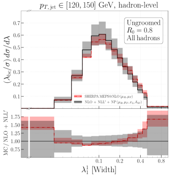
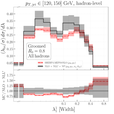
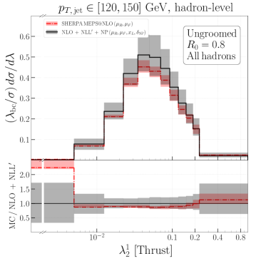
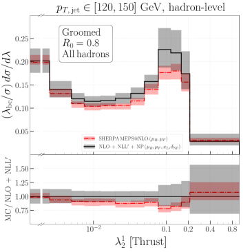
Figure 13: Comparison of hadron-level predictions from S HERPA (MEPS@NLO), based on all final state hadrons, for ungroomed and groomed jet-angularities in $Zj$ production, with $p_{T,\text{jet}}\in[120,150]\;\text{GeV}$, with $\text{NLO}+\text{NLL}^{\prime}$ results corrected for non-perturbative effects. Here $\lambda_{\text{bc}}$ stands for the bin centre.

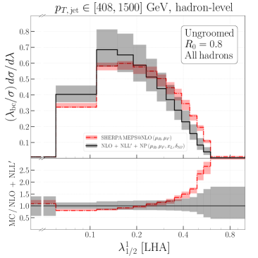
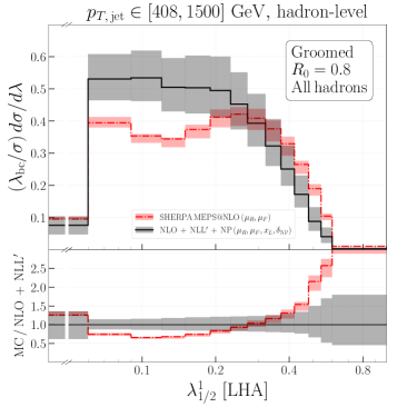
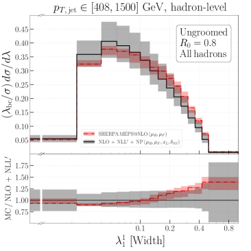
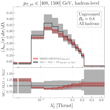
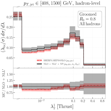
Figure 14: Comparison of hadron-level predictions from S HERPA (MEPS@NLO), based on all final state hadrons, for ungroomed and groomed jet-angularities in $Zj$ production, with $p_{T,\text{jet}}\in[408,1500]\;\text{GeV}$, with $\text{NLO}+\text{NLL}^{\prime}$ results corrected for non-perturbative effects. Here $\lambda_{\text{bc}}$ stands for the bin centre.

6 Conclusions and Outlook

In this paper we have performed a detailed phenomenological analysis of variables that describe the internal structure of jets produced in association with a $Z$ boson decaying into muons. Our study has focussed on IRC safe jet angularities that are characterised by an angular exponent $\alpha$, the variation of which allows us to probe QCD radiation in different ways. In particular, inspired by an upcoming measurement by the CMS collaboration, we have derived results for $\alpha=1/2,1,2$. Furthermore, we have considered standard (ungroomed) and groomed jets. Our grooming algorithm of choice has been SoftDrop ​​, which is characterised by the momentum fraction parameter $z_{\rm cut}$ and the angular exponent $\beta$. We have shown explicit results for the combination $z_{\rm cut}=0.1$, $\beta=0$, corresponding to the default choice of the CMS collaboration in their ongoing study.

Comparisons between unfolded experimental measurements and accurate first-principle theoretical predictions can allow us to test, and improve, our description of jet angularities. These observables are interesting for many reasons. For instance, they can be employed to distinguish quark-like from gluon-like jets, in a theoretically well-defined way (Badger:2016bpw, ; Gras:2017jty, ; Amoroso:2020lgh, ). They can also be used to extract Standard Model parameters, such as the strong coupling constant (Bendavid:2018nar, ). Furthermore, jet-angularity measurements can form an important input to constrain Monte Carlo event generators in general and the tuning of non-perturbative model parameters in particular (Amoroso:2020lgh, ).

The first part of the paper has been devoted to a detailed comparison of different MC event generators that provide an increasing sophistication in the way they include fixed-order matrix elements. In the region of small angularities, where soft radiation, both of perturbative and non-perturbative origin, dominates, we have confirmed that the spread in the predictions provided by widely used general-purpose event generators is largely reduced when grooming is considered. In our study we have also investigated the impact of fixed-order corrections to the parton shower. In particular, we have compared LO predictions from P YTHIA and H ERWIG , to the ones obtained with merged samples from S HERPA , both at LO and NLO. The inclusion of full NLO QCD corrections in the S HERPA MEPS@NLO simulations leads to a significant reduction of systematic uncertainties, estimated by consistent variations of the factorisation and renormalisation scales in both the matrix element and parton-shower components. When comparing to the LO simulations, we have observed noticeable effects at large values of the angularities, ranging from $\sim 10\%$ at moderate transverse momentum to $\sim 30\%$ in the high-$p_{T,\text{jet}}$ region. This applies to both, standard and groomed jets. This behaviour is perhaps related to an analogous trend observed in the inclusive $K$-factors, which are increasing functions of the jet transverse momentum. Our findings underline the importance of using state-of-the-art generators for jet phenomenology, especially when considering processes characterised by fairly large radiative corrections, as the one considered here, i.e. hadronic $Zj$ production.

The second part of this study has instead focussed on all-order predictions obtained with resummed perturbation theory at single-logarithmic accuracy. Thanks to a flavour-dependent matching to fixed-order predictions, we have been able to achieve $\text{NLO}+\text{NLL}^{\prime}$ accuracy. This includes, for the ungroomed case, the resummation of non-global logarithms, which we perform in the large-$N_{c}$ limit. The resummed and matched calculations are implemented in the resummation plugin to S HERPA . This allows us to exploit the main features of the event generation framework, including phase-space integration, matrix-element evaluations and matching, obtaining $\text{NLO}+\text{NLL}^{\prime}$ predictions that include fiducial cuts and can be faithfully compared to unfolded measurements. To this end, we complemented our perturbative predictions with non-perturbative corrections, derived from MC simulations, both for angularity measurements based on all or charged-only jet constituents. As expected, groomed jets benefit from smaller corrections, which however remain rather large for the $\lambda^{1}_{1/2}$ angularity. Although we have focussed on one particular combination of SoftDrop parameters, our resummed calculation is more general. It applies for all $\beta\geq 0$ values and can be extended to negative $\beta$ if SoftDrop is used in tagging rather than grooming mode. If one wanted to consider much smaller values of $z_{\rm cut}$, in addition the systematic resummation of related logarithmic corrections should be included. Similarly, for large values of $z_{\rm cut}$, power corrections can become important and should be included.

The main deliverable of this paper are $\text{NLO}+\text{NLL}^{\prime}$ predictions for jet angularities in $Z$+jets events in proton–proton collisions that can be immediately exploited for data–theory comparisons. However, this work has already shown us the path towards higher precision that we need to pursue. In this context, we can identify four complementary lines of research. First of all, although we do not expect large corrections, one should improve the accuracy of the resummation, in order to reduce the theoretical uncertainty. The framework for NNLL calculations has been worked out using SCET, although explicit results only exist, to the best of our knowledge, for the case $\alpha=2$ (Frye:2016okc, ; Frye:2016aiz, ). Second, it would be desirable to match the resummation to NNLO distributions. However, we recognise that this endeavour is much more formidable as it requires calculating $Z$ plus two partons at NNLO accuracy. Some first steps have however already been taken in this direction Hartanto:2019uvl ; Abreu:2020jxa ; Canko:2020ylt ; Badger:2021nhg . Next, given that the size of non-perturbative corrections can remain large even for groomed angularities, e.g. for $\alpha<1$, it would be interesting to study additional grooming strategies, such as complementing the SoftDrop procedure with a filtering step Butterworth:2008iy or using the Recursive SoftDrop algorithm Dreyer:2018tjj , although these tools would most likely further complicate the structure of the analytic resummation. Finally, a SCET framework to deal with non-perturbative effects has been recently developed (Hoang:2019ceu, ; Pathak:2020iue, ) and it would be interesting to quantitatively compare its predictions to the phenomenological model employed here.

Appendix A Additional results

In this Appendix, we collect supplementary results.

A.1 Numerical effects of the global and non-global soft function for groomed observables

In Fig. 15 we show the same results as in Fig. 4 in the main text, but with grooming.

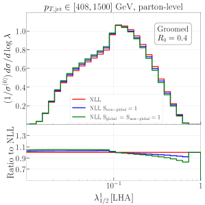
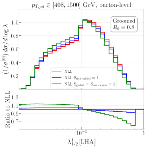
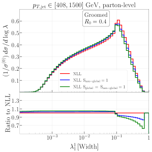
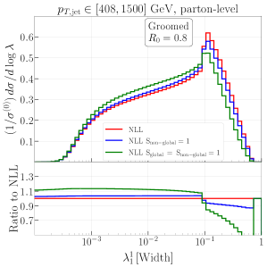
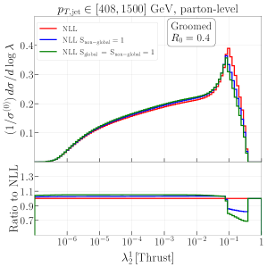
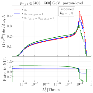
Figure 15: Same as Fig. 4 but with soft-drop grooming using $z_{\text{cut}}=0.1$, $\beta=0$.

A.2 Hadron-level predictions based on charged particles only

In Figs. 16 and 17 we provide $\text{NLO}+\text{NLL}^{\prime}$ + NP predictions for the jet angularities based on the charged jet constituents only for the two considered $p_{T,\text{jet}}$ slices, i.e. $p_{T,\text{jet}}\in[120,150]\;\text{GeV}$ and $p_{T,\text{jet}}\in[408,1500]\;\text{GeV}$. The corresponding correction factors have been presented in Fig. 12 in Section 5.2. The predictions are compared to MEPS@NLO results from S HERPA .

A.3 Hadron-level results for $R_{0}=0.4$ jets

Here we provide results analogous to the ones presented in Section 5.2 but for a smaller jet radius, namely $R_{0}=0.4$ jets. In particular, we show $\text{NLO}+\text{NLL}^{\prime}$ predictions, including non-perturbative corrections, and compare them to S HERPA MEPS@NLO results. This is done for the case of all-hadrons in Figs. 18 and 19 for the two considered transverse momentum slices, respectively, while in Figs. 20 and 21 we present corresponding results based on charged hadrons only.

The comparison yields very similar findings to the $R_{0}=0.8$ case reported in the main text. However, for the groomed width in the lower transverse momentum slice we here observe very large non-perturbative corrections (with corresponding large uncertainties). This signals the breakdown of our approximate treatment for including non-perturbative corrections. Here we probe a region of phase space close to the parton-shower cutoffs, below which the Monte Carlo simulations are purely determined by non-perturbative effects and, consequently, the hadron-to-parton-level ratios get large. This effect becomes more important as we lower $p_{T,\text{jet}}$ and/or the jet radius $R_{0}$. Its onset can be estimated using Eqs. (35) and (36).

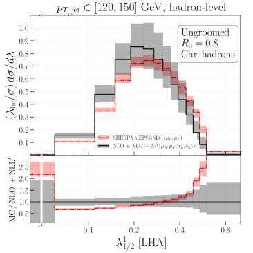
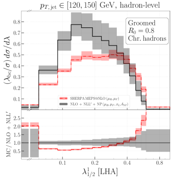
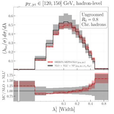
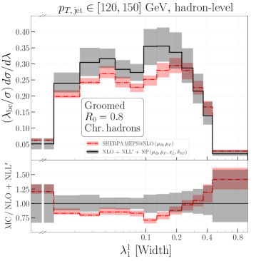
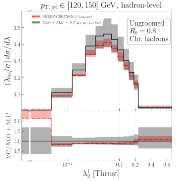
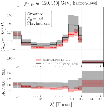
Figure 16: Comparison of hadron-level predictions from S HERPA (MEPS@NLO), based on charged hadrons only, for ungroomed and groomed jet-angularities in $Zj$ production, with $p_{T,\text{jet}}\in[120,150]\;\text{GeV}$, with $\text{NLO}+\text{NLL}^{\prime}$ results corrected for non-perturbative effects. Here $\lambda_{\text{bc}}$ stands for the bin centre.

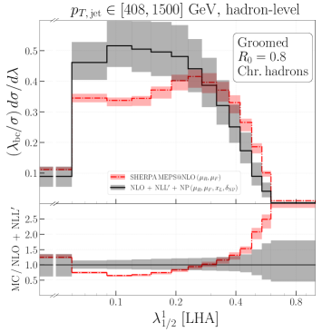
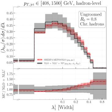
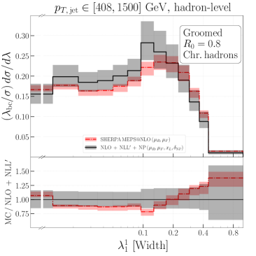
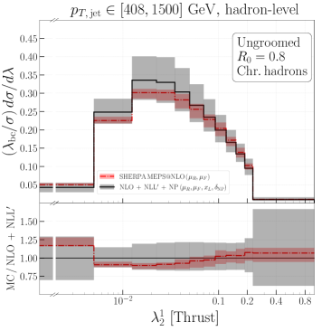
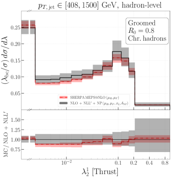
Figure 17: Comparison of hadron-level predictions from S HERPA (MEPS@NLO), based on charged hadrons only, for ungroomed and groomed jet-angularities in $Zj$ production, with $p_{T,\text{jet}}\in[408,1500]\;\text{GeV}$, with $\text{NLO}+\text{NLL}^{\prime}$ results corrected for non-perturbative effects. Here $\lambda_{\text{bc}}$ stands for the bin centre.

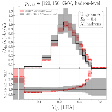
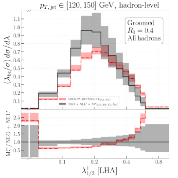
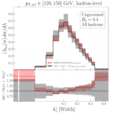
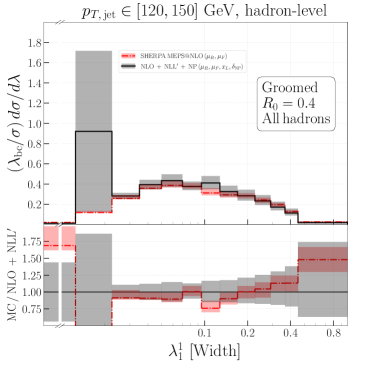
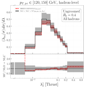
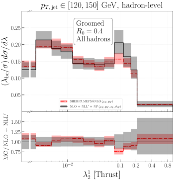
Figure 18: Same as Fig. 13 but for $R_{0}=0.4$ jets.

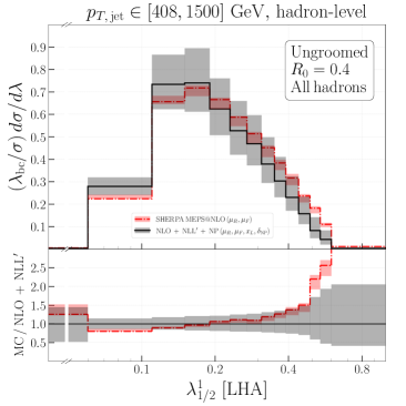
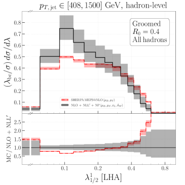
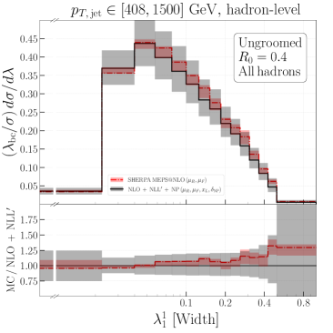
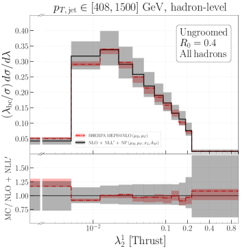
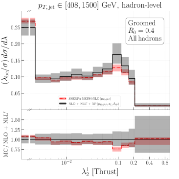
Figure 19: Same as Fig. 14 but for $R_{0}=0.4$ jets.

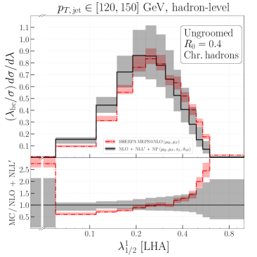
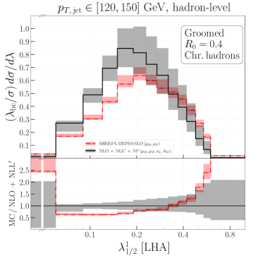
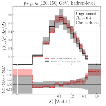
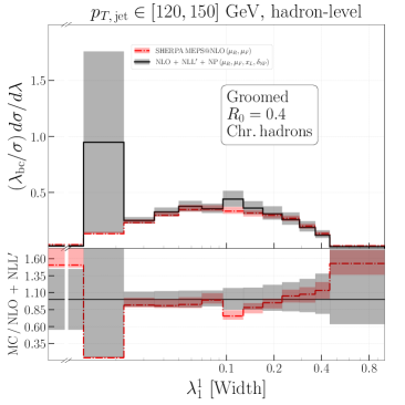
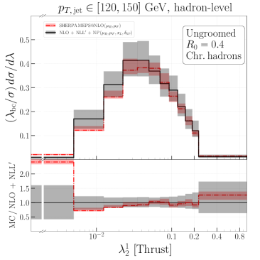
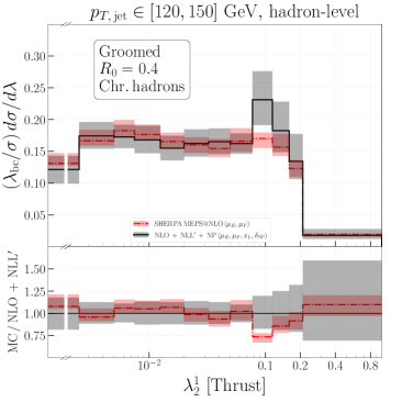
Figure 20: Same as Fig. 16 but for $R_{0}=0.4$ jets.

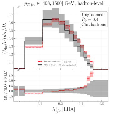
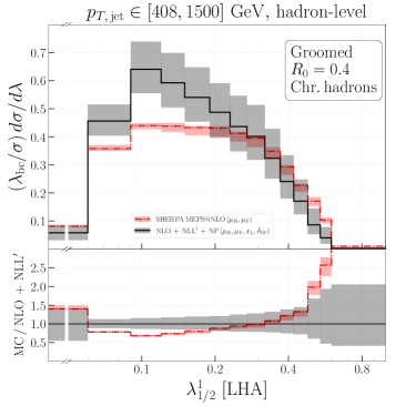
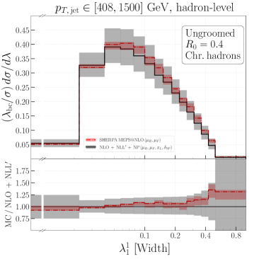
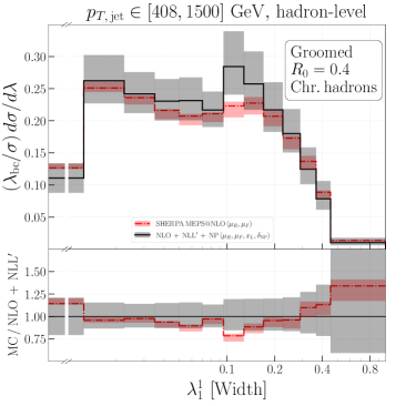
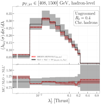
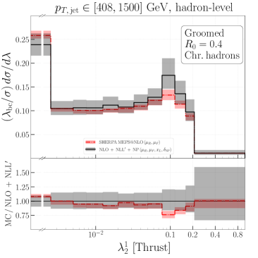
Figure 21: Same as Fig. 17 but for $R_{0}=0.4$ jets.

References

- (1) A. J. Larkoski, I. Moult, and B. Nachman, Jet Substructure at the Large Hadron Collider: A Review of Recent Advances in Theory and Machine Learning, Phys. Rept. 841 (2020) 1–63, [arXiv:1709.04464].
- (2) A. Butter et al., The Machine Learning Landscape of Top Taggers, SciPost Phys. 7 (2019) 014, [arXiv:1902.09914].
- (3) L. Benato, P. L. S. Connor, G. Kasieczka, D. Krücker, and M. Meyer, Teaching machine learning with an application in collider particle physics, JINST 15 (2020), no. 09 C09011.
- (4) D. Britzger, K. Rabbertz, D. Savoiu, G. Sieber, and M. Wobisch, Determination of the strong coupling constant using inclusive jet cross section data from multiple experiments, Eur. Phys. J. C79 (2019), no. 1 68, [arXiv:1712.00480].
- (5) CMS Collaboration, S. Chatrchyan et al., Measurement of the Ratio of the Inclusive 3-Jet Cross Section to the Inclusive 2-Jet Cross Section in pp Collisions at = 7 TeV and First Determination of the Strong Coupling Constant in the TeV Range, Eur. Phys. J. C73 (2013), no. 10 2604, [arXiv:1304.7498].
- (6) ATLAS Collaboration, M. Aaboud et al., Determination of the strong coupling constant from transverse energy–energy correlations in multijet events at using the ATLAS detector, Eur. Phys. J. C77 (2017), no. 12 872, [arXiv:1707.02562].
- (7) ATLAS Collaboration, G. Aad et al., Measurement of transverse energy-energy correlations in multi-jet events in collisions at TeV using the ATLAS detector and determination of the strong coupling constant , Phys. Lett. B750 (2015) 427–447, [arXiv:1508.01579].
- (8) CMS Collaboration, V. Khachatryan et al., Measurement of the inclusive 3-jet production differential cross section in proton–proton collisions at 7 TeV and determination of the strong coupling constant in the TeV range, Eur. Phys. J. C75 (2015), no. 5 186, [arXiv:1412.1633].
- (9) ATLAS Collaboration, G. Aad et al., Determination of the parton distribution functions of the proton from ATLAS measurements of differential and boson production in association with jets, arXiv:2101.05095.
- (10) ATLAS Collaboration, G. Aad et al., Measurement of the inclusive jet cross section in pp collisions at sqrt(s)=2.76 TeV and comparison to the inclusive jet cross section at sqrt(s)=7 TeV using the ATLAS detector, Eur. Phys. J. C73 (2013), no. 8 2509, [arXiv:1304.4739].
- (11) CMS Collaboration, V. Khachatryan et al., Constraints on parton distribution functions and extraction of the strong coupling constant from the inclusive jet cross section in pp collisions at TeV, Eur. Phys. J. C75 (2015), no. 6 288, [arXiv:1410.6765].
- (12) CMS Collaboration, V. Khachatryan et al., Measurement and QCD analysis of double-differential inclusive jet cross sections in pp collisions at TeV and cross section ratios to 2.76 and 7 TeV, JHEP 03 (2017) 156, [arXiv:1609.05331].
- (13) R. Abdul Khalek et al., Phenomenology of NNLO jet production at the LHC and its impact on parton distributions, Eur. Phys. J. C80 (2020), no. 8 797, [arXiv:2005.11327].
- (14) L. A. Harland-Lang, A. D. Martin, and R. S. Thorne, The Impact of LHC Jet Data on the MMHT PDF Fit at NNLO, Eur. Phys. J. C78 (2018), no. 3 248, [arXiv:1711.05757].
- (15) J. Pumplin, J. Huston, H. L. Lai, P. M. Nadolsky, W.-K. Tung, and C. P. Yuan, Collider Inclusive Jet Data and the Gluon Distribution, Phys. Rev. D80 (2009) 014019, [arXiv:0904.2424].
- (16) B. J. A. Watt, P. Motylinski, and R. S. Thorne, The Effect of LHC Jet Data on MSTW PDFs, Eur. Phys. J. C74 (2014) 2934, [arXiv:1311.5703].
- (17) M. Dasgupta and G. P. Salam, Resummation of nonglobal QCD observables, Phys. Lett. B512 (2001) 323–330, [hep-ph/0104277].
- (18) M. Dasgupta and G. P. Salam, Accounting for coherence in interjet E(t) flow: A Case study, JHEP 03 (2002) 017, [hep-ph/0203009].
- (19) M. Dasgupta, A. Fregoso, S. Marzani, and G. P. Salam, Towards an understanding of jet substructure, JHEP 09 (2013) 029, [arXiv:1307.0007].
- (20) M. Dasgupta, A. Fregoso, S. Marzani, and A. Powling, Jet substructure with analytical methods, Eur. Phys. J. C73 (2013), no. 11 2623, [arXiv:1307.0013].
- (21) A. J. Larkoski, S. Marzani, G. Soyez, and J. Thaler, Soft Drop, JHEP 05 (2014) 146, [arXiv:1402.2657].
- (22) M. Dasgupta, L. Schunk, and G. Soyez, Jet shapes for boosted jet two-prong decays from first-principles, JHEP 04 (2016) 166, [arXiv:1512.00516].
- (23) G. P. Salam, L. Schunk, and G. Soyez, Dichroic subjettiness ratios to distinguish colour flows in boosted boson tagging, JHEP 03 (2017) 022, [arXiv:1612.03917].
- (24) M. Dasgupta, A. Powling, L. Schunk, and G. Soyez, Improved jet substructure methods: Y-splitter and variants with grooming, JHEP 12 (2016) 079, [arXiv:1609.07149].
- (25) M. Dasgupta, A. Powling, and A. Siodmok, On jet substructure methods for signal jets, JHEP 08 (2015) 079, [arXiv:1503.01088].
- (26) A. J. Larkoski, I. Moult, and D. Neill, Power Counting to Better Jet Observables, JHEP 12 (2014) 009, [arXiv:1409.6298].
- (27) A. J. Larkoski, I. Moult, and D. Neill, Analytic Boosted Boson Discrimination, JHEP 05 (2016) 117, [arXiv:1507.03018].
- (28) A. J. Larkoski, Improving the understanding of jet grooming in perturbation theory, JHEP 09 (2020) 072, [arXiv:2006.14680].
- (29) A. J. Larkoski, G. P. Salam, and J. Thaler, Energy Correlation Functions for Jet Substructure, JHEP 06 (2013) 108, [arXiv:1305.0007].
- (30) Z.-B. Kang, K. Lee, X. Liu, D. Neill, and F. Ringer, The soft drop groomed jet radius at NLL, JHEP 02 (2020) 054, [arXiv:1908.01783].
- (31) P. Cal, D. Neill, F. Ringer, and W. J. Waalewijn, Calculating the angle between jet axes, JHEP 04 (2020) 211, [arXiv:1911.06840].
- (32) P. Cal, K. Lee, F. Ringer, and W. J. Waalewijn, Jet energy drop, JHEP 11 (2020) 012, [arXiv:2007.12187].
- (33) S. Marzani, G. Soyez, and M. Spannowsky, Looking inside jets: an introduction to jet substructure and boosted-object phenomenology, arXiv:1901.10342. [Lect. Notes Phys.958,pp.(2019)].
- (34) A. J. Larkoski, J. Thaler, and W. J. Waalewijn, Gaining (Mutual) Information about Quark/Gluon Discrimination, JHEP 11 (2014) 129, [arXiv:1408.3122].
- (35) J. R. Andersen et al., Les Houches 2015: Physics at TeV Colliders Standard Model Working Group Report, in 9th Les Houches Workshop on Physics at TeV Colliders (PhysTeV 2015) Les Houches, France, June 1-19, 2015, 2016. arXiv:1605.04692.
- (36) P. Gras, S. Höche, D. Kar, A. Larkoski, L. Lönnblad, S. Plätzer, A. Siodmok, P. Skands, G. Soyez, and J. Thaler, Systematics of quark/gluon tagging, JHEP 07 (2017) 091, [arXiv:1704.03878].
- (37) S. Amoroso et al., Les Houches 2019: Physics at TeV Colliders: Standard Model Working Group Report, in 11th Les Houches Workshop on Physics at TeV Colliders: PhysTeV Les Houches, 3, 2020. arXiv:2003.01700.
- (38) J. R. Andersen et al., Les Houches 2017: Physics at TeV Colliders Standard Model Working Group Report, in 10th Les Houches Workshop on Physics at TeV Colliders: PhysTeV Les Houches, 3, 2018. arXiv:1803.07977.
- (39) E. Gerwick, S. Höche, S. Marzani, and S. Schumann, Soft evolution of multi-jet final states, JHEP 02 (2015) 106, [arXiv:1411.7325].
- (40) S. D. Ellis, C. K. Vermilion, J. R. Walsh, A. Hornig, and C. Lee, Jet Shapes and Jet Algorithms in SCET, JHEP 11 (2010) 101, [arXiv:1001.0014].
- (41) A. Hornig, Y. Makris, and T. Mehen, Jet Shapes in Dijet Events at the LHC in SCET, JHEP 04 (2016) 097, [arXiv:1601.01319].
- (42) Z.-B. Kang, K. Lee, and F. Ringer, Jet angularity measurements for single inclusive jet production, JHEP 04 (2018) 110, [arXiv:1801.00790].
- (43) Z.-B. Kang, K. Lee, X. Liu, and F. Ringer, Soft drop groomed jet angularities at the LHC, Phys. Lett. B 793 (2019) 41–47, [arXiv:1811.06983].
- (44) M. Cacciari, G. P. Salam, and G. Soyez, The anti- jet clustering algorithm, JHEP 04 (2008) 063, [arXiv:0802.1189].
- (45) C. F. Berger, T. Kucs, and G. F. Sterman, Event shape / energy flow correlations, Phys.Rev. D68 (2003) 014012, [hep-ph/0303051].
- (46) L. G. Almeida, S. J. Lee, G. Perez, G. F. Sterman, I. Sung, and J. Virzi, Substructure of high- Jets at the LHC, Phys. Rev. D79 (2009) 074017, [arXiv:0807.0234].
- (47) A. Banfi, G. P. Salam, and G. Zanderighi, Principles of general final-state resummation and automated implementation, JHEP 03 (2005) 073, [hep-ph/0407286].
- (48) A. J. Larkoski, D. Neill, and J. Thaler, Jet Shapes with the Broadening Axis, JHEP 04 (2014) 017, [arXiv:1401.2158].
- (49) S. Marzani, L. Schunk, and G. Soyez, A study of jet mass distributions with grooming, JHEP 07 (2017) 132, [arXiv:1704.02210].
- (50) CMS Collaboration, Study of quark and gluon jet substructure in dijet and Z+jet events from pp collisions, Tech. Rep. CMS-PAS-SMP-20-010, CERN, Geneva, 2021.
- (51) M. Rubin, G. P. Salam, and S. Sapeta, Giant QCD K-factors beyond NLO, JHEP 09 (2010) 084, [arXiv:1006.2144].
- (52) A. Buckley et al., General-purpose event generators for LHC physics, Phys. Rept. 504 (2011) 145–233, [arXiv:1101.2599].
- (53) J. M. Campbell and R. K. Ellis, An Update on vector boson pair production at hadron colliders, Phys. Rev. D 60 (1999) 113006, [hep-ph/9905386].
- (54) J. M. Campbell, R. K. Ellis, and C. Williams, Vector boson pair production at the LHC, JHEP 07 (2011) 018, [arXiv:1105.0020].
- (55) R. Boughezal, J. M. Campbell, R. K. Ellis, C. Focke, W. Giele, X. Liu, F. Petriello, and C. Williams, Color singlet production at NNLO in MCFM, Eur. Phys. J. C 77 (2017), no. 1 7, [arXiv:1605.08011].
- (56) P. Nason, A New method for combining NLO QCD with shower Monte Carlo algorithms, JHEP 11 (2004) 040, [hep-ph/0409146].
- (57) S. Frixione, P. Nason, and C. Oleari, Matching NLO QCD computations with Parton Shower simulations: the POWHEG method, JHEP 11 (2007) 070, [arXiv:0709.2092].
- (58) S. Alioli, P. Nason, C. Oleari, and E. Re, A general framework for implementing NLO calculations in shower Monte Carlo programs: the POWHEG BOX, JHEP 06 (2010) 043, [arXiv:1002.2581].
- (59) S. Frixione and B. R. Webber, Matching NLO QCD computations and parton shower simulations, JHEP 06 (2002) 029, [hep-ph/0204244].
- (60) J. Alwall, R. Frederix, S. Frixione, V. Hirschi, F. Maltoni, O. Mattelaer, H. S. Shao, T. Stelzer, P. Torrielli, and M. Zaro, The automated computation of tree-level and next-to-leading order differential cross sections, and their matching to parton shower simulations, JHEP 07 (2014) 079, [arXiv:1405.0301].
- (61) S. Höche, F. Krauss, M. Schönherr, and F. Siegert, QCD matrix elements + parton showers: The NLO case, JHEP 04 (2013) 027, [arXiv:1207.5030].
- (62) T. Gleisberg, S. Höche, F. Krauss, M. Schönherr, S. Schumann, F. Siegert, and J. Winter, Event generation with SHERPA 1.1, JHEP 02 (2009) 007, [arXiv:0811.4622].
- (63) Sherpa Collaboration, E. Bothmann et al., Event Generation with Sherpa 2.2, SciPost Phys. 7 (2019), no. 3 034, [arXiv:1905.09127].
- (64) NNPDF Collaboration, R. D. Ball et al., Parton distributions for the LHC Run II, JHEP 04 (2015) 040, [arXiv:1410.8849].
- (65) S. Schumann and F. Krauss, A Parton shower algorithm based on Catani-Seymour dipole factorisation, JHEP 03 (2008) 038, [arXiv:0709.1027].
- (66) S. Actis, A. Denner, L. Hofer, J.-N. Lang, A. Scharf, and S. Uccirati, RECOLA: REcursive Computation of One-Loop Amplitudes, Comput. Phys. Commun. 214 (2017) 140–173, [arXiv:1605.01090].
- (67) B. Biedermann, S. Bräuer, A. Denner, M. Pellen, S. Schumann, and J. M. Thompson, Automation of NLO QCD and EW corrections with Sherpa and Recola, Eur. Phys. J. C77 (2017) 492, [arXiv:1704.05783].
- (68) A. Denner, S. Dittmaier, and L. Hofer, Collier: a fortran-based Complex One-Loop LIbrary in Extended Regularizations, Comput. Phys. Commun. 212 (2017) 220–238, [arXiv:1604.06792].
- (69) S. Höche, F. Krauss, S. Schumann, and F. Siegert, QCD matrix elements and truncated showers, JHEP 05 (2009) 053, [arXiv:0903.1219].
- (70) S. Catani, F. Krauss, R. Kuhn, and B. R. Webber, QCD matrix elements + parton showers, JHEP 11 (2001) 063, [hep-ph/0109231].
- (71) E. Bothmann, M. Schönherr, and S. Schumann, Reweighting QCD matrix-element and parton-shower calculations, Eur. Phys. J. C76 (2016), no. 11 590, [arXiv:1606.08753].
- (72) M. Cacciari, S. Frixione, M. L. Mangano, P. Nason, and G. Ridolfi, The t anti-t cross-section at 1.8-TeV and 1.96-TeV: A Study of the systematics due to parton densities and scale dependence, JHEP 04 (2004) 068, [hep-ph/0303085].
- (73) J.-C. Winter, F. Krauss, and G. Soff, A Modified cluster hadronization model, Eur. Phys. J. C36 (2004) 381–395, [hep-ph/0311085].
- (74) T. Sjöstrand and M. van Zijl, A Multiple Interaction Model for the Event Structure in Hadron Collisions, Phys. Rev. D36 (1987) 2019.
- (75) J. Bellm et al., Herwig 7.0/Herwig++ 3.0 release note, Eur. Phys. J. C76 (2016), no. 4 196, [arXiv:1512.01178].
- (76) J. Bellm et al., Herwig 7.2 release note, Eur. Phys. J. C80 (2020), no. 5 452, [arXiv:1912.06509].
- (77) T. Sjöstrand, S. Ask, J. R. Christiansen, R. Corke, N. Desai, P. Ilten, S. Mrenna, S. Prestel, C. O. Rasmussen, and P. Z. Skands, An introduction to PYTHIA 8.2, Comput. Phys. Commun. 191 (2015) 159–177, [arXiv:1410.3012].
- (78) S. Plätzer and S. Gieseke, Dipole Showers and Automated NLO Matching in Herwig++, Eur. Phys. J. C 72 (2012) 2187, [arXiv:1109.6256].
- (79) J. Bellm, S. Gieseke, and S. Plätzer, Merging NLO Multi-jet Calculations with Improved Unitarization, Eur. Phys. J. C 78 (2018), no. 3 244, [arXiv:1705.06700].
- (80) A. Buckley, J. Butterworth, D. Grellscheid, H. Hoeth, L. Lonnblad, J. Monk, H. Schulz, and F. Siegert, Rivet user manual, Comput. Phys. Commun. 184 (2013) 2803–2819, [arXiv:1003.0694].
- (81) C. Bierlich et al., Robust Independent Validation of Experiment and Theory: Rivet version 3, SciPost Phys. 8 (2020) 026, [arXiv:1912.05451].
- (82) M. Cacciari, G. P. Salam, and G. Soyez, FastJet User Manual, Eur. Phys. J. C72 (2012) 1896, [arXiv:1111.6097].
- (83) CMS Collaboration, A. M. Sirunyan et al., Measurements of the differential jet cross section as a function of the jet mass in dijet events from proton-proton collisions at TeV, JHEP 11 (2018) 113, [arXiv:1807.05974].
- (84) S. Marzani, D. Reichelt, S. Schumann, G. Soyez, and V. Theeuwes, Fitting the Strong Coupling Constant with Soft-Drop Thrust, JHEP 11 (2019) 179, [arXiv:1906.10504].
- (85) N. Baberuxki, C. T. Preuss, D. Reichelt, and S. Schumann, Resummed predictions for jet-resolution scales in multijet production in annihilation, JHEP 04 (2020) 112, [arXiv:1912.09396].
- (86) J. Baron, D. Reichelt, S. Schumann, N. Schwanemann, and V. Theeuwes, Soft-drop grooming for hadronic event shapes, arXiv:2012.09574.
- (87) T. Gleisberg and S. Höche, Comix, a new matrix element generator, JHEP 12 (2008) 039, [arXiv:0808.3674].
- (88) T. Gleisberg and F. Krauss, Automating dipole subtraction for QCD NLO calculations, Eur. Phys. J. C53 (2008) 501–523, [arXiv:0709.2881].
- (89) F. Cascioli, P. Maierhofer, and S. Pozzorini, Scattering Amplitudes with Open Loops, Phys. Rev. Lett. 108 (2012) 111601, [arXiv:1111.5206].
- (90) M. Dasgupta, K. Khelifa-Kerfa, S. Marzani, and M. Spannowsky, On jet mass distributions in Z+jet and dijet processes at the LHC, JHEP 10 (2012) 126, [arXiv:1207.1640].
- (91) M. Dasgupta, F. A. Dreyer, K. Hamilton, P. F. Monni, G. P. Salam, and G. Soyez, Parton showers beyond leading logarithmic accuracy, Phys. Rev. Lett. 125 (2020), no. 5 052002, [arXiv:2002.11114].
- (92) A. Banfi and M. Dasgupta, Problems in resumming interjet energy flows with clustering, Phys. Lett. B628 (2005) 49–56, [hep-ph/0508159].
- (93) Y. Delenda, R. Appleby, M. Dasgupta, and A. Banfi, On QCD resummation with k(t) clustering, JHEP 12 (2006) 044, [hep-ph/0610242].
- (94) A. Banfi, M. Dasgupta, K. Khelifa-Kerfa, and S. Marzani, Non-global logarithms and jet algorithms in high-pT jet shapes, JHEP 08 (2010) 064, [arXiv:1004.3483].
- (95) Y. Delenda and K. Khelifa-Kerfa, On the resummation of clustering logarithms for non-global observables, JHEP 09 (2012) 109, [arXiv:1207.4528].
- (96) A. Lifson, G. P. Salam, and G. Soyez, Calculating the primary Lund Jet Plane density, JHEP 10 (2020) 170, [arXiv:2007.06578].
- (97) A. Banfi, G. P. Salam, and G. Zanderighi, Infrared safe definition of jet flavor, Eur. Phys. J. C47 (2006) 113–124, [hep-ph/0601139].
- (98) C. Frye, A. J. Larkoski, M. D. Schwartz, and K. Yan, Factorization for groomed jet substructure beyond the next-to-leading logarithm, JHEP 07 (2016) 064, [arXiv:1603.09338].
- (99) S. Höche, D. Reichelt, and F. Siegert, Momentum conservation and unitarity in parton showers and NLL resummation, JHEP 01 (2018) 118, [arXiv:1711.03497].
- (100) C. F. Berger, T. Kucs, and G. F. Sterman, Interjet energy flow / event shape correlations, Int. J. Mod. Phys. A 18 (2003) 4159–4168, [hep-ph/0212343].
- (101) ATLAS Collaboration, G. Aad et al., Light-quark and gluon jet discrimination in collisions at with the ATLAS detector, Eur. Phys. J. C 74 (2014), no. 8 3023, [arXiv:1405.6583].
- (102) M. Dasgupta, L. Magnea, and G. P. Salam, Non-perturbative QCD effects in jets at hadron colliders, JHEP 02 (2008) 055, [arXiv:0712.3014].
- (103) S. Marzani, L. Schunk, and G. Soyez, The jet mass distribution after Soft Drop, Eur. Phys. J. C78 (2018), no. 2 96, [arXiv:1712.05105].
- (104) T. Sjöstrand, Multiple Parton-Parton Interactions in Hadronic Events, in Proceedings, 23RD International Conference on High Energy Physics, JULY 16-23, 1986, Berkeley, CA, 1985.
- (105) T. Sjöstrand and P. Z. Skands, Multiple interactions and the structure of beam remnants, JHEP 03 (2004) 053, [hep-ph/0402078].
- (106) M. Bähr, S. Gieseke, and M. H. Seymour, Simulation of multiple partonic interactions in Herwig++, JHEP 07 (2008) 076, [arXiv:0803.3633].
- (107) S. Gieseke, F. Loshaj, and P. Kirchgaeßer, Soft and diffractive scattering with the cluster model in Herwig, Eur. Phys. J. C77 (2017), no. 3 156, [arXiv:1612.04701].
- (108) B. Andersson, G. Gustafson, G. Ingelman, and T. Sjöstrand, Parton Fragmentation and String Dynamics, Phys. Rept. 97 (1983) 31–145.
- (109) T. Sjöstrand, Jet Fragmentation of Nearby Partons, Nucl. Phys. B248 (1984) 469–502.
- (110) B. R. Webber, A QCD Model for Jet Fragmentation Including Soft Gluon Interference, Nucl. Phys. B238 (1984) 492–528.
- (111) A. Kupco, Cluster hadronization in HERWIG 5.9, in Monte Carlo generators for HERA physics. Proceedings, Workshop, Hamburg, Germany, 1998-1999, pp. 292–300, 1998. hep-ph/9906412.
- (112) C. Frye, A. J. Larkoski, M. D. Schwartz, and K. Yan, Precision physics with pile-up insensitive observables, arXiv:1603.06375.
- (113) H. B. Hartanto, S. Badger, C. Brønnum-Hansen, and T. Peraro, A numerical evaluation of planar two-loop helicity amplitudes for a W-boson plus four partons, JHEP 09 (2019) 119, [arXiv:1906.11862].
- (114) S. Abreu, H. Ita, F. Moriello, B. Page, W. Tschernow, and M. Zeng, Two-Loop Integrals for Planar Five-Point One-Mass Processes, JHEP 11 (2020) 117, [arXiv:2005.04195].
- (115) D. D. Canko, C. G. Papadopoulos, and N. Syrrakos, Analytic representation of all planar two-loop five-point Master Integrals with one off-shell leg, JHEP 01 (2021) 199, [arXiv:2009.13917].
- (116) S. Badger, H. B. Hartanto, and S. Zoia, Two-loop QCD corrections to production at hadron colliders, arXiv:2102.02516.
- (117) J. M. Butterworth, A. R. Davison, M. Rubin, and G. P. Salam, Jet substructure as a new Higgs search channel at the LHC, Phys. Rev. Lett. 100 (2008) 242001, [arXiv:0802.2470].
- (118) F. A. Dreyer, L. Necib, G. Soyez, and J. Thaler, Recursive Soft Drop, JHEP 06 (2018) 093, [arXiv:1804.03657].
- (119) A. H. Hoang, S. Mantry, A. Pathak, and I. W. Stewart, Nonperturbative Corrections to Soft Drop Jet Mass, JHEP 12 (2019) 002, [arXiv:1906.11843].
- (120) A. Pathak, I. W. Stewart, V. Vaidya, and L. Zoppi, EFT for Soft Drop Double Differential Cross Section, JHEP 04 (2021) 032, [arXiv:2012.15568].
- (121) J. D. Hunter, Matplotlib: A 2D Graphics Environment, Comput. Sci. Eng. 9 (2007), no. 3 90–95.
- (122) T. Oliphant, Guide to NumPy. Trelgol Publishing, 2006.