A Quantum Convolutional Neural Network on NISQ Devices

Abstract

Quantum machine learning is one of the most promising applications of quantum computing in the Noisy Intermediate-Scale Quantum(NISQ) era. Here we propose a quantum convolutional neural network(QCNN) inspired by convolutional neural networks(CNN), which greatly reduces the computing complexity compared with its classical counterparts, with $O((log_{2}M)^{6})$ basic gates and $O(m^{2}+e)$ variational parameters, where $M$ is the input data size, $m$ is the filter mask size and $e$ is the number of parameters in a Hamiltonian. Our model is robust to certain noise for image recognition tasks and the parameters are independent on the input sizes, making it friendly to near-term quantum devices. We demonstrate QCNN with two explicit examples . First, QCNN is applied to image processing and numerical simulation of three types of spatial filtering, image smoothing, sharpening, and edge detection are performed. Secondly, we demonstrate QCNN in recognizing image, namely, the recognition of handwritten numbers. Compared with previous work, this machine learning model can provide implementable quantum circuits that accurately corresponds to a specific classical convolutional kernel. It provides an efficient avenue to transform CNN to QCNN directly and opens up the prospect of exploiting quantum power to process information in the era of big data.

I Introduction

Machine learning has fundamentally transformed the way people think and behave. Convolutional Neural Network(CNN) is an important machine learning model which has the advantage of utilizing the correlation information of data, with many interesting applications ranging from image recognition to precision medicine.

Quantum information processing (QIP)^{1, 2}, which exploits quantum-mechanical phenomena such as quantum superpositions and quantum entanglement, allows one to overcome the limitations of classical computation and reaches higher computational speed for certain problems^{3, 4, 5}. Quantum machine learning, as an interdisciplinary study between machine learning and quantum information, has undergone a flurry of developments in recent years^{6, 7, 8, 9, 10, 11, 12, 13, 14, 15}. Machine learning algorithm consists of three components: representation, evaluation and optimization, and the quantum version^{16, 17, 18, 19, 20} usually concentrates on realizing the evaluation part, the fundamental construct in deep learning²¹.

A CNN generally consists of three layers, convolution layers, pooling layers and fully connected layers. The convolution layer calculates new pixel values $x_{ij}^{(\ell)}$ from a linear combination of the neighborhood pixels in the preceding map with the specific weights, $x_{i,j}^{(\ell)}=\sum_{a,b=1}^{m}w_{a,b}x_{i+a-2,j+b-2}^{(\ell-1)}$, where the weights $w_{a,b}$ form a $m\times m$ matrix named as a convolution kernel or a filter mask. Pooling layer reduces feature map size, e.g. by taking the average value from four contiguous pixels, and are often followed by application of a nonlinear (activation) function. The fully connected layer computes the final output by a linear combination of all remaining pixels with specific weights determined by parameters in a fully connected layer. The weights in the filter mask and fully connected layer are optimized by training on large datasets.

In this article, we demonstrate the basic framework of a quantum convolutional neural network(QCNN) by sequentially realizing convolution layers, pooling layers and fully connected layers. Firstly, we implement convolution layers based on linear combination of unitary operators(LCU)^{22, 23, 24}. Secondly, we abandon some qubits in the quantum circuit to simulate the effect of the classical pooling layer. Finally, the fully connected layer is realized by measuring the expectation value of a parametrized Hamiltonian and then a nonlinear (activation) function to post-process the expectation value. We perform numerical demonstrations with two examples to show the validity of our algorithm. Finally, the computing complexity of our algorithm is discussed followed by a summary.

II Framework of Quantum Neural Networks

II.1 Quantum Convolution Layer

Figure 1: Comparison of classical convolution processing and quantum convolution processing. $F$ and $G$ are the input and output image data, respectively. On the classical computer, a $M\times M$ image can be represented as a matrix and encoded with at least $2^{n}$ bits [$n=\lceil\log_{2}(M^{2})\rceil$]. The classical image transformation through the convolution layer is performed by matrix computation $F*W$, which leads to $x_{i,j}^{(\ell)}=\sum_{a,b=1}^{m}w_{a,b}x_{i+a-2,j+b-2}^{(\ell-1)}$. The same image can be represented as a quantum state and encoded in at least $n$ qubits on a quantum computer. The quantum image transformation is realized by the unitary evolution $U$ on a specific quantum state.

The first step for performing quantum convolution layer is to encode the image data into a quantum system. In this work, we encode the pixel positions in the computational basis states and the pixel values in the probability amplitudes, forming a pure quantum state. Given a 2D image $F=(F_{i,j})_{M\times L}$, where $F_{i,j}$ represents the pixel value at position $(i,j)$ with $i=1,\dots,M$ and $j=1,\dots,L$. $F$ is transformed as a vector $\vec{f}$ with $ML$ elements by puting the first column of $F$ into the first $M$ elements of $\vec{f}$, the second column the next $M$ elements , etc. That is,

$$\vec{f}=(F_{1,1},F_{2,1},\dots,F_{M,1},F_{1,2},\dots,F_{i,j},\dots,F_{M,L})^{T}.$$ (1)

Accordingly, the image data $\vec{f}$ can be mapped onto a pure quantum state $|f\rangle=\sum_{k=0}^{2^{n}-1}c_{k}|k\rangle$ with $n=\lceil\log_{2}(ML)\rceil$ qubits, where the computational basis $|k\rangle$ encodes the position $(i,j)$ of each pixel, and the coefficient $c_{k}$ encodes the pixel value, i.e., $c_{k}=F_{i,j}/(\sum{F_{i,j}^{2}})^{1/2}$ for $k<ML$ and $c_{k}=0$ for $k\geq ML$. Here $(\sum{F_{i,j}^{2}})^{1/2}$ is a constant factor to normalizing the quantum state.

Without loss of generality, we focus on the input image with $M=L=2^{n}$ pixels. The convolution layer transforms an input image $F=(F_{i,j})_{M\times M}$ into an output image $G=(G_{i,j})_{M\times M}$ by a specific filter mask $W$. In the quantum context, this linear transformation, corresponding to a specific spatial filter operation, can be represented as $|g\rangle=U|f\rangle$ with the input image state $|f\rangle$ and the output image state $|g\rangle$. For simplicity, we take a $3\times 3$ filter mask as an example

$$W=\left[\begin{matrix}w_{11}&w_{12}&w_{13}\\ w_{21}&w_{22}&w_{23}\\ w_{31}&w_{32}&w_{33}\\ \end{matrix}\right].$$ (2)

The generalization to arbitrary $m\times m$ filter mask is straightforward. Convolution operation will transform the input image $F=(F_{i,j})_{M\times M}$ into the output image as $G=(G_{i,j})_{M\times M}$ with the pixel $G_{i,j}=\sum_{u,v=1}^{3}w_{uv}F_{i+u-2,j+v-2}$ ($2\leq i,j\leq M-1$). The corresponding quantum evolution $U|f\rangle$ can be performed as follows. We represent input image $F=(F_{i,j})_{M\times M}$ as an initial state

$$|f\rangle=\sum_{k=0}^{M^{2}-1}c_{k}|k\rangle,$$ (3)

where $c_{k}=F_{i,j}/(\sum{F_{i,j}^{2}})^{1/2}$. The $M^{2}\times M^{2}$ linear filtering operator $U$ can be defined as²⁵:

$$U=\left[\begin{matrix}E&&&&&\\ V_{1}&V_{2}&V_{3}&&&\\ &\ddots&\ddots&\ddots&&\\ &&\ddots&\ddots&\ddots&\\ &&&V_{1}&V_{2}&V_{3}\\ &&&&&E\\ \end{matrix}\right],$$ (4)

where $E$ is an $M$ dimensional identity matrix, and $V_{1}$, $V_{2}$, $V_{3}$ are $M\times M$ matrices defined by

$$V_{1}=\left(\begin{array}[]{ccccc}0&&&&\\ w_{11}&w_{21}&w_{31}&&\\ &\ddots&\ddots&\ddots&\\ &&w_{11}&w_{21}&w_{31}\\ &&&&0\\ \end{array}\right)_{M\times M}V_{2}=\left(\begin{array}[]{ccccc}1&&&&\\ w_{12}&w_{22}&w_{32}&&\\ &\ddots&\ddots&\ddots&\\ &&w_{12}&w_{22}&w_{32}\\ &&&&1\\ \end{array}\right)_{M\times M}V_{3}=\left(\begin{array}[]{ccccc}0&&&&\\ w_{13}&w_{23}&w_{33}&&\\ &\ddots&\ddots&\ddots&\\ &&w_{13}&w_{23}&w_{33}\\ &&&&0\\ \end{array}\right)_{M\times M}.$$ (5)

Generally speaking, the linear filtering operator $U$ is non-unitary that can not be performed directly. Actually, we can embed $U$ in a bigger system with an ancillary system and decompose it into a linear combination of four unitary operators ²⁶. $U=U_{1}+U_{2}+U_{3}+U_{4}$, where $U_{1}=(U+U^{\dagger})/2+i\sqrt{I-(U+U^{\dagger})^{2}/4}$, $U_{2}=(U+U^{\dagger})/2-i\sqrt{I-(U+U^{\dagger})^{2}/4}$, $U_{3}=(U-U^{\dagger})/2i+i\sqrt{I+(U-U^{\dagger})^{2}/4}$ and $U_{4}=(U-U^{\dagger})/2i-i\sqrt{I+(U-U^{\dagger})^{2}/4}$. However, the basic gates consumed to perform $U_{i}$ scale exponentially in the dimensions of quantum systems, making the quantum advantage diminishing. Therefore, we present a new approach to construct the filter operator to reduce the gate complexity. For convenience, we change the elements of the first row, the last row, the first column and the last column in the matrix $V_{1},V_{2},$ and $V_{3}$, which is allowable in imagining processing, to the following form

$$V^{\prime}_{1}=\left(\begin{array}[]{ccccc}w_{21}&w_{31}&&&w_{11}\\ w_{11}&w_{21}&w_{31}&&\\ &\ddots&\ddots&\ddots&\\ &&w_{11}&w_{21}&w_{31}\\ w_{31}&&&w_{11}&w_{21}\\ \end{array}\right)_{M\times M}V^{\prime}_{2}=\left(\begin{array}[]{ccccc}w_{22}&w_{32}&&&w_{12}\\ w_{12}&w_{22}&w_{32}&&\\ &\ddots&\ddots&\ddots&\\ &&w_{12}&w_{22}&w_{32}\\ w_{32}&&&w_{12}&w_{22}\\ \end{array}\right)_{M\times M}V^{\prime}_{3}=\left(\begin{array}[]{ccccc}w_{23}&w_{33}&&&w_{13}\\ w_{13}&w_{23}&w_{33}&&\\ &\ddots&\ddots&\ddots&\\ &&w_{13}&w_{23}&w_{33}\\ w_{33}&&&w_{13}&w_{23}\\ \end{array}\right)_{M\times M}.$$ (6)

Defining the adjusted linear filtering operator $U^{\prime}$ as

$$U^{\prime}=\left[\begin{matrix}V^{\prime}_{2}&V^{\prime}_{3}&&&&V^{\prime}_{1}\\ V^{\prime}_{1}&V^{\prime}_{2}&V^{\prime}_{3}&&&\\ &\ddots&\ddots&\ddots&&\\ &&\ddots&\ddots&\ddots&\\ &&&V^{\prime}_{1}&V^{\prime}_{2}&V^{\prime}_{3}\\ V^{\prime}_{3}&&&&V^{\prime}_{1}&V^{\prime}_{2}\\ \end{matrix}\right],$$ (7)

Next, we decompose $V^{\prime}_{\mu}(\mu=1,2,3)$ into three unitary matrices without normalization, $V^{\prime}_{\mu}=V^{\prime}_{1\mu}+V^{\prime}_{2\mu}+V^{\prime}_{3\mu}$, where

$$V^{\prime}_{1\mu}=\left(\begin{array}[]{ccccc}&&&&w_{1\mu}\\ w_{1\mu}&&&&\\ \ddots&\ddots&\ddots&&\\ &&w_{1\mu}&&\\ &&&w_{1\mu}&\\ \end{array}\right)_{M\times M}\\ V^{\prime}_{2\mu}=\left(\begin{array}[]{ccccc}w_{2\mu}&&&&\\ &w_{2\mu}&&&\\ &\ddots&\ddots&\ddots&\\ &&&w_{2\mu}&\\ &&&&w_{2\mu}\\ \end{array}\right)_{M\times M}\\ V^{\prime}_{3\mu}=\left(\begin{array}[]{ccccc}&w_{3\mu}&&&\\ &&w_{3\mu}&&\\ &&\ddots\ddots&\ddots&\\ &&&&w_{3\mu}\\ w_{3\mu}&&&&\\ \end{array}\right)_{M\times M}.$$ (8)

Thus, the linear filtering operator $U^{\prime}$ can be expressed as

$$U^{\prime}=\sum_{\mu=1}^{3}\sum_{v=1}^{3}(V^{\prime}_{\mu\mu}/w_{\mu\mu})\otimes V^{\prime}_{v\mu}.$$ (9)

which can be simplified to

$$U^{\prime}=\sum_{k=1}^{9}\beta_{k}Q_{k},$$ (10)

where $Q_{k}=(V^{\prime}_{\mu\mu}/w_{\mu\mu})\otimes V^{\prime}_{v\mu}/w_{v\mu}$ is unitary, and $\beta_{k}$ is a relabelling of the indices.

Now, we can perform $U^{\prime}$ through the linear combination of unitary operators $Q_{k}$. The number of unitary operators is equal to the size of filter mask. The quantum circuit to realize $U^{\prime}$ is shown in Fig.2. The work register $|f\rangle$ and four ancillary qubits $|0000\rangle_{a}$ are entangled together to form a bigger system.

Firstly, we prepare the initial state $|f\rangle$ using amplitude encoding method or quantum random access memory(qRAM). Then, performing unitary matrix $S$ on the ancillary registers to transform $|0000\rangle_{a}$ into a specific superposition state $|\psi\rangle_{a}$

$$S|0000\rangle_{a}=|\psi\rangle_{a}=\sum_{v=1}^{9}\beta_{k}/N|k\rangle$$ (11)

where $N_{c}=\sqrt{\sum_{k=1}^{9}\beta_{k}^{2}}$ and $S$ satisfies

$$S_{k,1}=\begin{cases}\beta_{k}/N_{c}&\textrm{if $k\leq 9$}\\ 0&\textrm{if $k>9$.}\end{cases}$$ (12)

$S$ is a parameter matrix corresponding to a specific filter mask that realizes a specific task.

Then, we implement a series of ancillary system controlled operations $Q_{k}\otimes|k\rangle\langle k|$ on the work system $|f\rangle$ to realize LCU. Nextly, Hadamard gates $H^{T}=H^{\otimes 4}$ are acted to uncompute the ancillary registers $|\psi\rangle_{a}$. The state is transformed to

$$|g^{\prime}\rangle=\sum_{i=1}^{16}\frac{1}{N_{c}}|i\rangle\sum_{k=1}^{16}H^{T}_{(i:)}S_{(:1)}Q_{k}|f\rangle,$$ (13)

where $H^{T}_{(i:)}$ is the i-th row in matrix $H^{T}$ and $S_{(:1)}$ is the first column in matrix $S$. The first term equals to

$$\frac{1}{N_{c}}|0\rangle\sum_{k=1}^{9}\beta_{k}Q_{k}|f\rangle,$$ (14)

which corresponds to the filter mask $W$. The $i$-th term equals to filter mask $W^{i}(i=2,3,\dots,16)$, where

$$W^{i}=\left[\begin{matrix}H^{T}_{i1}w_{11}&H^{T}_{i4}w_{12}&H^{T}_{i7}w_{13}\\ H^{T}_{i2}w_{21}&H^{T}_{i5}w_{22}&H^{T}_{i8}w_{23}\\ H^{T}_{i3}w_{31}&H^{T}_{i6}w_{32}&H^{T}_{i9}w_{33}\\ \end{matrix}\right].$$ (15)

Totally, $16$ filter masks are realized, corresponding to ancilla qubits in $16$ different state $|i\rangle(i=1,2,\dots,16)$. Therefore, the whole effect of evolution on state $|f\rangle$ without considering the ancilla qubits, is the linear combination of the effects of 16 filter masks.

If we only need one filter mask $W$, measuring the ancillary register and conditioned on seeing $|0000\rangle$. We have the state $\frac{1}{N_{c}}|0000\rangle U^{\prime}|f\rangle$, which is proportional to our expected result state $|g\rangle$. The probability of detecting the ancillary state $|0000\rangle$ is

$$P_{s}=\parallel\sum_{k=1}^{9}\beta_{k}Q_{k}|f\rangle\parallel^{2}/{N_{c}^{2}}$$ (16)

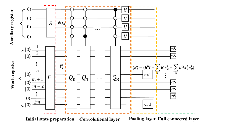
Figure 2: Quantum circuit for realizing the QCNN. $|f\rangle$ denotes the initial state of work system after encoded the image data, and the ancillary system is a four qubits system in the $|0000\rangle_{a}$ state. The squares represent unitary operations and the circles represent the state of the controlling system. Unitary operations $Q_{1}$,$Q_{2}$,$\cdots$, $Q_{9}$, are activated only when the auxiliary system is in state $|0000\rangle$,$|0001\rangle$$\cdots$,$|1000\rangle$ respectively.

After obtaining the final result $\frac{1}{N_{c}}U^{\prime}|f\rangle$, we can multiply the constant factor $N_{c}$ to compute $|g^{\prime}\rangle=U^{\prime}|f\rangle$. In conclusion, the filter operator $U^{\prime}$ can be decomposed into a linear combination of nine unitary operators in the case that the general filter mask is $W$. Only four qubits or a nine energy level ancillary system is consumed to realize the general filter operator $U^{\prime}$, which is independent on the dimensions of image size.

The final stage of our method is to extract useful information from the processed results $|g^{\prime}\rangle$. Clearly, the image state $|g\rangle$ is different from $|g^{\prime}\rangle$. However, not all elements in $|f\rangle$ are evaluated, the elements corresponding to the four edges of original image remain unchanged. One is only interested in the pixel values which are evaluated by $W$ in $|f\rangle$. These pixel values in $|g^{\prime}\rangle$ are as same as that in $|g\rangle$(see proof in supplementary materials). So, we can obtain the informations of $G=(G_{i,j})_{M\times M}$ ($2\leq i,j\leq M-1$) by evaluating the $|f\rangle$ under operator $U^{\prime}$ instead of $U$.

II.2 Quantum Pooling Layer

The function of pooling layer after the convolutional layer is to reduce the spatial size of the representation so as to reduce the amount of parameters. We adopt average pooling which calculates the average value for each patch on the feature map as pooling layers in our model. Consider a $2*2$ pixels pooling operation applied with a stride of 2 pixels. It can be directly realized by ignoring the last qubit and the $m$-th qubit in quantum context. The input image $|g^{\prime}\rangle=(g_{1},g_{2},g_{3},g_{4},\dots,\dots,g_{M^{2}})^{T}$ after this operation can be expressed as the output image

$$|p\rangle=\left(\sqrt{g_{1}^{2}+g_{2}^{2}+g_{M+1}^{2}+g_{M+2}^{2}},\sqrt{g_{3}^{2}+g_{4}^{2}+g_{M+3}^{2}+g_{M+4}^{2}},\dots,\sqrt{g_{M^{2}-M-1}^{2}+g_{M^{2}-M}^{2}+g_{M^{2}-1}^{2}+g_{M}^{2}}\right)^{T}.$$ (17)

II.3 Quantum Fully Connected Layer

Fully connected layers complie the data extracted by previous layers to form the final output, it usually appear at the end of convolutional neural networks. We define a parametrized Hamiltonian as the quantum fully connected layer. This Hamiltonian consists of identity operators $I$ and Pauli operators $\sigma_{z}$,

$$\mathcal{H}=h^{0}I+\sum_{i}h^{i}\sigma_{z}^{i}+\sum_{i,j}h^{ij}\sigma_{z}^{i}\sigma_{z}^{j}+\dots$$ (18)

where $h^{0},h^{i},h^{ij},\cdots$ are the parameters, and Roman indices $i,j$ denote the qubit on which the operator acts, i.e., $\sigma^{i}_{z}$ means Pauli matrix $\sigma_{z}$ acting on a qubit at site $i$. We measure the expectation value of the parametrized Hamiltonian $f(p)=\langle{p}|\mathcal{H}|p\rangle$. $f(p)$ is the final output of the whole quantum neural network. Then, we add an active function to nonlinearly map $f(p)$ to $R(f(p))$. The parameters in Hamiltonian matrix $\mathcal{H}$ are updated by gradient descent method, i.e., are calculated by $\frac{\partial f(p)}{\partial h^{i}}=\langle{p}|\sigma_{z}^{i}|p\rangle$ and $\frac{\partial f(p)}{\partial h^{ij}}=\langle{p}|\sigma_{z}^{i}\sigma_{z}^{j}|p\rangle$. The parameters in $S$ matrix can be trained through classical backpropagation.

Now, we construct the framework of quantum neural networks. We demonstrate the performance of our method in image processing and handwritten number recognition in the next section.

III Numerical Simulations

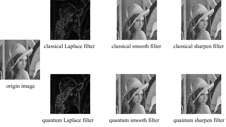
Figure 3: Three types of image processing, edge detection, image smoothing and sharpening, are implemented on an image by classical method and quantum method respectively.

III.1 Image Processing: Edge Detection, Image Smoothing and Sharpening

In addition to constructing QCNN, the quantum convolutional layer can also be used to spatial filtering which is a technique for image processing^{27, 28, 29, 25}, such as image smoothing, sharpening, edge detection and edge enhancement. To show the quantum convolutional layer can handle various image processing tasks, we demonstrate three types of image processing, edge detection, image smoothing and sharpening with fixed filter mask $W_{de}$, $W_{sm}$ and $W_{sh}$ respectively

$$W_{de}=\left(\begin{array}[]{ccc}-1&-1&-1\\ -1&8&-1\\ -1&-1&-1\\ \end{array}\right),\\ W_{sm}=\frac{1}{13}\left(\begin{array}[]{ccc}1&1&1\\ 1&5&1\\ 1&1&1\\ \end{array}\right),\\ W_{sh}=\frac{1}{16}\left(\begin{array}[]{ccc}-2&-2&-2\\ -2&32&-2\\ -2&-2&-2\\ \end{array}\right).$$ (19)

In a spatial image processing task, we only need one specific filter mask. Therefore, after performing the above quantum convolutional layer mentioned, we measure the ancillary register. If we obtain $|0\rangle$, our algorithm succeeds and the spatial filtering task is completed. The numerical simulation proves that the output images transformed by a classical and quantum convolutional layer are exactly the same, as shown in Fig.(3).

III.2 Handwritten Number Recognition

Here we demonstrate a type of image recognition task on a real-world dataset, called MNIST, a handwritten character dataset. In this case, we simulate a complete quantum convolutional neural network model, including a convolutional layer, a pooling layer, and a full-connected layer, as shown in Fig.(2). We consider the two-class image recognition task(recognizing handwritten characters ${}^{\prime}1^{\prime}$ and ${}^{\prime}8^{\prime}$) and ten-class image recognition task(recognizing handwritten characters ${}^{\prime}0^{\prime}$-${}^{\prime}9^{\prime}$). Meanwhile, considering the noise on NISQ quantum system, we respectively simulate two circumstances that are the quantum gate $Q_{k}$ is a perfect gate or a gate with certain noise. The noise is simulated by randomly acting a single qubit Pauli gate in $[I,X,Y,Z]$ with a probability of $0.01$ on the quantum circuit after an operation implemented. In detail, the handwritten character image of MNIST has $28\times 28$ pixels. For convenience, we expand $0$ at the edge of the initial image until $32\times 32$ pixels. Thus, the work register of QCNN consists of 10 qubits and the ancillary register needs 4 qubits. The convolutional layer is characterized by 9 learnable parameters in matrix $W$, that is the same for QCNN and CNN. In QCNN, by abandoning the $4$-th and $9$-th qubit of the work register, we perform the pooling layer on quantum circuit. In CNN, we perform average pooling layer directly. Through measuring the expected values of different Hamiltonians on the remaining work qubits, we can obtain the measurement values. After putting them in an activation function, we get the final classification result. In CNN, we perform a two-layer fully connected neural network and an activation function. In the two-classification problem, the QCNN’s parametrized Hamiltonian has 37 learnable parameters and the CNN’s fully-connected layer has 256 learnable parameters. The classification result that is close to 0 are classified as handwritten character ${}^{\prime}1^{\prime}$, and that is close to 1 are classified as handwritten character ${}^{\prime}8^{\prime}$. In the ten-classification problem, the parametrized Hamiltonian has $10\times 37$ learnable parameters and the CNN’s fully-connected layer has $10\times 256$ learnable parameters. The result is a 10-dimension vector. The classification results are classified as the index of the max element of the vector. Details of parameters, accuracy and gate complexity are listed in Table.(1).

For the 2 class classification problem, the training set and test set have a total of 5000 images and 2100 images, respectively. For the 10 class classification problem, the training set and test set have a total of 60000 images and 10000 images, respectively. Because in a training process, 100 images are randomly chosen in one epoch, and 50 epochs in total, the accuracy of the training set and the test set will fluctuate. So, we repeatedly execute noisy QCNN, noise-free, and CNN 100 times, under the same construction. In this way, we obtain the average accuracy and the field of accuracy, as shown in Fig.(4). We can conclude that from the numerical simulation result, QCNN and CNN provide similar performance. QCNN involves fewer parameters and has a smaller fluctuation range.

Table 1: The important parameters of models

Models	Problems	Data Set	Parameters
			Learnable Parameters	Average Accuracy	Gate Complexity
Noisy QCNN	${}^{\prime}1^{\prime}$ or ${}^{\prime}8^{\prime}$	training set	46	0.948	$O((log_{2}M)^{6})$
		test set		0.960
	${}^{\prime}0^{\prime}\sim^{\prime}9^{\prime}$	training set	379	0.742
		test set		0.740
Noise-free QCNN	${}^{\prime}1^{\prime}$ or ${}^{\prime}8^{\prime}$	training set	46	0.954
		test set		0.963
	${}^{\prime}0^{\prime}\sim^{\prime}9^{\prime}$	training set	379	0.756
		test set		0.743
CNN	${}^{\prime}1^{\prime}$ or ${}^{\prime}8^{\prime}$	training set	265	0.962	$O(M^{2})$
		test set		0.972
	${}^{\prime}0^{\prime}\sim^{\prime}9^{\prime}$	training set	2569	0.802
		test set		0.804

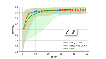
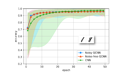
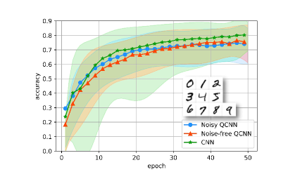
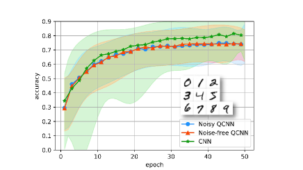
Figure 4: The performance of QCNN based on MNIST. The blue, red, and green curves denote the average accuracy of the noisy QCNN, noise-free QCNN, and CNN, respectively. The shadow areas of the corresponding color denote the accuracy fluctuation range in the 100 times simulation results. The insets are the typical images from MNIST set. (a), (b) are the curves representing the result from the training set and the test set for the 2 class classification problem respectively. (c), (d) show the result from the training set and the test set for the 10 class classification problem respectively.

IV Algorithm complexity

We analyze the computing resources in gate complexity and qubit consumption. (1) Gate complexity. At the convolutional layer stage, we could prepare an initial state in $O(poly(log_{2}(M^{2}))$ steps. In the case of preparing a particular input $|f\rangle$, we employ the amplitude encoding method in Ref.^{30, 31, 32}. It was shown that if the amplitude $c_{k}$ and $P_{k}=\sum_{k}|c_{k}|^{2}$ can be efficiently calculated by a classical algorithm, constructing the $log_{2}(M^{2})$-qubit $X$ state takes $O(poly(log_{2}(M^{2}))$ steps. Alternatively, we can resort to quantum random access memory^{33, 34, 35}. Quantum Random Access Memory (qRAM) is an efficient method to do state preparation, whose complexity is $O(log_{2}(M^{2}))$ after the quantum memory cell established. Moreover, the controlled operations $Q_{k}$ can be decomposed into $O((log_{2}M)^{6})$ basic gates (see details in Appendix A). In summary, our algorithm uses $O((log_{2}M)^{6})$ basic steps to realize the filter progress in the convolutional layer. For CNN, the complexity of implementing a classical convolutional layer is $O(M^{2})$. Thus, this algorithm achieves an exponential speedup over classical algorithms in gate complexity. The measurement complexity in fully connected layers is $O(e)$, where $e$ is the number of parameters in the Hamiltonian.
(2) Memory consumption. The ancillary qubits in the whole algorithm are $O(log_{2}(m^{2}))$, where $m$ is the dimension of the filter mask, and the work qubits are $O(log_{2}(M^{2}))$. Thus, the total qubits resource needed is $O(log_{2}(m^{2})+O(log_{2}(M^{2})$.

V Conclusion

In summary, we desighed a quantum Neural Network which provides exponential speed-ups over their classical counterparts in gate complexity. With fewer parameters, our model achieves similar performance compared with classical algorithm in handwritten number recognition tasks. Therefore, this algorithm has significant advantages over the classical algorithms for large data. We present two interesting and practical applications, image processing and handwritten number recognition, to demonstrate the validity of our method. We give the mapping relations between a specific classical convolutional kernel to a quantum circuit, that provides a bridge between QCNN to CNN. It is a general algorithm and can be implemented on any programmable quantum computer, such as superconducting, trapped ions, and photonic quantum computer. In the big data era, this algorithm has great potential to outperform its classical counterpart, and works as an efficient solution.

Acknowledgements

Appendix A: Adjusted operator $U^{\prime}$ can provide enough information to remap the output imagine.

$Proof.$- The different elements of image matrix after implementing operator $U^{\prime}$ compared with $U$ are in the edges of image matrix. We prove that the evolution under operator $U^{\prime}$ can provide enough information to remap the output image. The different elements between $U^{\prime}$ and $U$ are included in

$$U^{\prime}_{k,n}\neq U_{k,n}\begin{cases}(1\leq k\leq M;1\leq n\leq 2M,M^{2}-M\leq n\leq M^{2})\\ (M^{2}-M\leq k\leq M^{2};1\leq n\leq M,M^{2}-3M\leq n\leq M^{2}-M)\\ (k=sM+1;n=1+(s-1)M,2+(s-1)M,sM,sM+1,sM+2,(s+1)M,(s+1)M+1,(s+1)M+2,(s+2)M)\\ (k=(s+1)M;n=1,sM-1,sM,sM+1,(s+1)M-2,(s+1)M-1,(s+1)M+1,(s+2)M-2,(s+2)M-1)\end{cases}$$ (20)

where $1\leq s\leq M-2$.

After performing $U^{\prime}$ and $U$ on quantum state $|f\rangle$ respectively, the difference exits in the elements $|g^{\prime}_{k}\rangle\neq|g_{k}\rangle(k=1,2,\cdots,M,sM+1,(s+1)M,M^{2}-M+1,\cdots,M^{2})$, where $1\leq s\leq M-2$. Since $|g^{\prime}\rangle$ can be remapped to $G^{\prime}$, $U^{\prime}$ will give the output image $G^{\prime}=(G^{\prime}_{i,j})_{M\times M}$. The elements in $U^{\prime}$ which is different from $U$ only affect the pixel $i,j\not\in{2,\cdots,M-1}$. Thus, only and if only $i,j\not\in{2,\cdots,M-1}$, the matrix elements satisfy $G_{i,j}\neq G^{\prime}_{i,j}$. Namely, the output imagine $G^{\prime}_{i,j}=G_{i,j}$($2\leq i,j\leq M-1$).

Appendix B: Decomposing operator Q into basic gates

Considering the nine operators $Q_{1}$, $Q_{2}$,$\cdots$, $Q_{9}$ consist of filter operator $U^{\prime}$. $Q_{k}$ is the tensor product of two of the following three operators

$$E_{1}=\left(\begin{array}[]{cccccc}&&&&1\\ 1&&&&\\ \ddots&\ddots&\ddots&&\\ &&1&&\\ &&&1&\\ \end{array}\right)_{M\times M}\\ E_{2}=\left(\begin{array}[]{cccccc}1&&&&\\ &1&&&\\ &\ddots&\ddots&\ddots&\\ &&&1&\\ &&&&1\\ \end{array}\right)_{M\times M}\\ E_{3}=\left(\begin{array}[]{cccccc}&1&&&\\ &&1&&\\ &&\ddots\ddots&\ddots&\\ &&&&1\\ 1&&&&\\ \end{array}\right)_{M\times M}.$$ (21)

$E_{2}$ is a $M\times M$ identity matrix not need to be further decomposed. For convenient, consider a $n$-qubits operator $E_{1}$ with dimension $M\times M$, where $n=log_{2}(M^{2})$. It can be expressed by the combination of $O(n^{3})$ CNOT gates and Pauli $X$ gates as shown in Fig.5. Consequently, $E_{3}$ can be decomposed into the inverse of combinations of basic gate as shown in Fig.5, because of the fact $E_{3}=E_{1}^{\dagger}$.

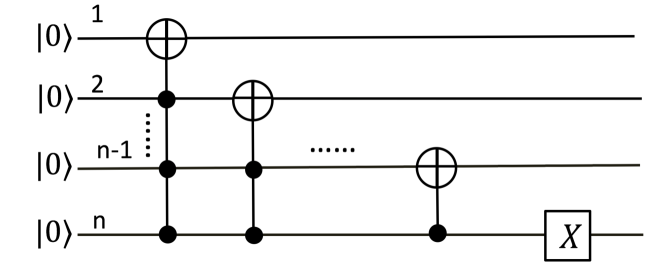
Figure 5: Decomposition of operator $E_{1}$ in the form of basic gates.

Thus, $Q_{k}$ can be implemented by no more than $O(n^{6})$ basic gates. Totally, the controlled $Q_{k}$ operation can be implemented by no more than $O(n^{6})=O((log_{2}M)^{6})$(ignoring constant number).

References

- 1 Paul Benioff. The computer as a physical system: A microscopic quantum mechanical hamiltonian model of computers as represented by turing machines. Journal of statistical physics, 22(5):563–591, 1980.
- 2 Richard P Feynman. Simulating physics with computers. International Journal of Theoretical Physics, 21(6):467–488, 1982.
- 3 Shor P. W. Polynomial-time algorithms for prime factorization and discrete logarithms on a quantum computer. 1995.
- 4 Lov K Grover. Quantum mechanics helps in searching for a needle in a haystack. Physical review letters, 79(2):325, 1997.
- 5 G. L. Long. Grover algorithm with zero theoretical failure rate. Phys. Rev. A, 64:022307, Jul 2001.
- 6 Jacob Biamonte, Peter Wittek, Nicola Pancotti, Patrick Rebentrost, Nathan Wiebe, and Seth Lloyd. Quantum machine learning. Nature, 549(7671):195–202, 2017.
- 7 Vedran Dunjko, Jacob M Taylor, and Hans J Briegel. Quantum-enhanced machine learning. Physical review letters, 117(13):130501, 2016.
- 8 Nathan Killoran, Thomas R Bromley, Juan Miguel Arrazola, Maria Schuld, Nicolás Quesada, and Seth Lloyd. Continuous-variable quantum neural networks. Physical Review Research, 1(3):033063, 2019.
- 9 Junhua Liu, Kwan Hui Lim, Kristin L Wood, Wei Huang, Chu Guo, and He-Liang Huang. Hybrid quantum-classical convolutional neural networks. arXiv preprint arXiv:1911.02998, 2019.
- 10 Feng Hu, Ban-Nan Wang, Ning Wang, and Chao Wang. Quantum machine learning with d-wave quantum computer. Quantum Engineering, 1(2):e12, 2019.
- 11 Edward Farhi, Hartmut Neven, et al. Classification with quantum neural networks on near term processors. Quantum Review Letters, 1(2 (2020)):10–37686, 2020.
- 12 William Huggins, Piyush Patil, Bradley Mitchell, K Birgitta Whaley, and E Miles Stoudenmire. Towards quantum machine learning with tensor networks. Quantum Science and technology, 4(2):024001, 2019.
- 13 Xiao Yuan, Jinzhao Sun, Junyu Liu, Qi Zhao, and You Zhou. Quantum simulation with hybrid tensor networks. arXiv preprint arXiv:2007.00958, 2020.
- 14 Yao Zhang and Qiang Ni. Recent advances in quantum machine learning. Quantum Engineering, 2(1):e34, 2020.
- 15 Jin-Guo Liu, Liang Mao, Pan Zhang, and Lei Wang. Solving quantum statistical mechanics with variational autoregressive networks and quantum circuits. Machine Learning: Science and Technology, 2(2):025011, 2021.
- 16 Edward Farhi and Hartmut Neven. Classification with quantum neural networks on near term processors. arXiv preprint arXiv:1802.06002, 2018.
- 17 Iris Cong, Soonwon Choi, and Mikhail D Lukin. Quantum convolutional neural networks. Nature Physics, 15(12):1273–1278, 2019.
- 18 Brian C Britt. Modeling viral diffusion using quantum computational network simulation. Quantum Engineering, 2(1):e29, 2020.
- 19 Maria Schuld and Nathan Killoran. Quantum machine learning in feature hilbert spaces. Physical review letters, 122(4):040504, 2019.
- 20 YaoChong Li, Ri-Gui Zhou, RuQing Xu, Jia Luo, and WenWen Hu. A quantum deep convolutional neural network for image recognition. Quantum Science and Technology, 5(4):044003, 2020.
- 21 Ian Goodfellow, Yoshua Bengio, Aaron Courville, and Yoshua Bengio. Deep learning, volume 1. MIT press Cambridge, 2016.
- 22 Long Gui-Lu. General quantum interference principle and duality computer. Communications in Theoretical Physics, 45(5):825, 2006.
- 23 Stan Gudder. Mathematical theory of duality quantum computers. Quantum Information Processing, 6(1):37–48, 2007.
- 24 Shi-Jie Wei and Gui-Lu Long. Duality quantum computer and the efficient quantum simulations. Quantum Information Processing, 15(3):1189–1212, 2016.
- 25 Xi-Wei Yao, Hengyan Wang, Zeyang Liao, Ming-Cheng Chen, Jian Pan, Jun Li, Kechao Zhang, Xingcheng Lin, Zhehui Wang, Zhihuang Luo, et al. Quantum image processing and its application to edge detection: theory and experiment. Physical Review X, 7(3):031041, 2017.
- 26 Tao Xin, Shijie Wei, Jianlian Cui, Junxiang Xiao, Iñigo Arrazola, Lucas Lamata, Xiangyu Kong, Dawei Lu, Enrique Solano, and Guilu Long. Quantum algorithm for solving linear differential equations: Theory and experiment. Physical Review A, 101(3):032307, 2020.
- 27 Fei Yan, Abdullah M Iliyasu, and Salvador E Venegas-Andraca. A survey of quantum image representations. Quantum Information Processing, 15(1):1–35, 2016.
- 28 Salvador E Venegas-Andraca and Sougato Bose. Storing, processing, and retrieving an image using quantum mechanics. In Quantum Information and Computation, volume 5105, pages 137–147. International Society for Optics and Photonics, 2003.
- 29 Phuc Q Le, Fangyan Dong, and Kaoru Hirota. A flexible representation of quantum images for polynomial preparation, image compression, and processing operations. Quantum Information Processing, 10(1):63–84, 2011.
- 30 Gui-Lu Long and Yang Sun. Efficient scheme for initializing a quantum register with an arbitrary superposed state. Physical Review A, 64(1):014303, 2001.
- 31 Lov Grover and Terry Rudolph. Creating superpositions that correspond to efficiently integrable probability distributions. arXiv preprint quant-ph/0208112, 2002.
- 32 Andrei N Soklakov and Rüdiger Schack. Efficient state preparation for a register of quantum bits. Physical review A, 73(1):012307, 2006.
- 33 Vittorio Giovannetti, Seth Lloyd, and Lorenzo Maccone. Quantum random access memory. Physical review letters, 100(16):160501, 2008.
- 34 Vittorio Giovannetti, Seth Lloyd, and Lorenzo Maccone. Architectures for a quantum random access memory. Physical Review A, 78(5):052310, 2008.
- 35 Srinivasan Arunachalam, Vlad Gheorghiu, Tomas Jochym-O’Connor, Michele Mosca, and Priyaa Varshinee Srinivasan. On the robustness of bucket brigade quantum ram. New Journal of Physics, 17(12):123010, 2015.