Scale without conformal invariance in membrane theory

Abstract

We investigate the relation between dilatation and conformal symmetries in the statistical mechanics of flexible crystalline membranes. We analyze, in particular, a well-known model which describes the fluctuations of a continuum elastic medium embedded in a higher-dimensional space. In this theory, the renormalization group flow connects a non-interacting ultraviolet fixed point, where the theory is controlled by linear elasticity, to an interacting infrared fixed point. By studying the structure of correlation functions and of the energy-momentum tensor, we show that, in the infrared, the theory is only scale-invariant: the dilatation symmetry is not enhanced to full conformal invariance. The model is shown to present a non-vanishing virial current which, despite being non-conserved, maintains a scaling dimension exactly equal to $D-1$, even in presence of interactions. We attribute the absence of anomalous dimensions to the symmetries of the model under translations and rotations in the embedding space, which are realized as shifts of phonon fields, and which protect the renormalization of several non-invariant operators. We also note that closure of a symmetry algebra with both shift symmetries and conformal invariance would require, in the hypothesis that phonons transform as primary fields, the presence of new shift symmetries which are not expected to hold on physical grounds. We then consider an alternative model, involving only scalar fields, which describes effective phonon-mediated interactions between local Gaussian curvatures. The model is described in the ultraviolet by two copies of the biharmonic theory, which is conformal, but flows in the infrared to a fixed point which we argue to be only dilatation-invariant.

1 Introduction

Asymptotic scale invariance plays a crucial role in quantum field theory, from statistical mechanics to models of fundamental interactions. In several cases, the asymptotically-emergent scaling symmetry is enlarged to full conformal invariance, which opens the way to powerful techniques such as bootstrap equations [1, 2] or, in two dimensions, methods based on the infinite Virasoro algebra [3]. These approaches give access to high-precision non-perturbative calculations and, in some cases, even to exact solutions. Understanding the conditions under which conformal symmetry arises is thus of great importance, and has motivated extensive investigations [4].

Particularly general results were established for two- and four-dimensional field theories assuming unitarity, or, in Euclidean space, the corresponding property of reflection positivity [5, 6, 7, 2]. In the two-dimensional case, Zamolodchikov and Polchinski proved that unitary scale-invariant field theories are always conformal under two mild assumptions: the existence of a well-defined energy-momentum tensor and the discreteness of the spectrum of operator dimensions [5, 6]. In four-dimensional space, a similar result is expected to hold [4], as indicated by perturbative proofs to all orders [8, 9, 10] and corroborated by non-perturbative evidences [4, 9, 11, 12, 13]. Some analogue derivations were argued to be applicable to unitary theories in any even dimension $D=2n$ [14].

These arguments, however, cannot be extended straightforwardly to arbitrary dimensions (possibly odd or non-integer) or to models lacking unitarity or reflection positivity. In addition, several derivations break down when the energy-momentum tensor and its two-point function are not well defined, which can happen in sigma models relevant for string theories [6, 15, 16]. Models with scale but without conformal invariance, in fact, exist and have been explicitly identified [4, 15, 6, 17, 18, 19, 20, 16, 21, 22], or indirectly conjectured based on holographic analyses [23, 24, 25]. Although unphysical in the context of fundamental interactions, models defined in general dimension $D$ and without unitarity or reflection positivity are recurrent in statistical mechanics. Analyses of the relation between scale and conformal invariance in more general classes of theories are thus crucial for several physical applications (see Refs. [26, 27, 28, 6, 29, 30, 2, 31] for some of the results and methods).

If we try to consider, roughly speaking, how likely it is for a scale-invariant model to exhibit conformal symmetry, we can often run into a dilemma. On the one hand, dilatation invariance is not a sufficient condition for the extended conformal invariance and, therefore, a generic scale-invariant theory can be expected to lack conformal symmetry. On the other hand, there exist arguments suggesting that, for interacting field theories, scale invariance should imply conformal invariance generically [19, 2, 31, 21]. A formulation of this reasoning starts from the structure of the energy-momentum tensor $T_{\alpha\beta}$ and its trace $T_{\alpha}^{\alpha}$. In local and scale-invariant theories, dilatation symmetry implies that $T_{\alpha}^{\alpha}=\partial_{\alpha}V^{\alpha}$, where $V^{\alpha}$ is a local field, the ’virial current’. Conformal invariance arises instead whenever $V^{\alpha}=j^{\alpha}+\partial_{\beta}L^{\alpha\beta}$ where $j^{\alpha}$ is conserved ($\partial_{\alpha}j^{\alpha}=0$) and $L^{\alpha\beta}$ is a tensor field [6]. Although the requirements for conformal symmetry are stronger and not automatically satisfied a priori, possible candidates for the virial current are constrained, because $V^{\alpha}$ must have a scaling dimension exactly equal to $\{V^{\alpha}\}=D-1$ in order to match the dimensions of the energy-momentum tensor $\{T_{\alpha\beta}\}=D$ [19, 2, 31, 21]. All vector currents are usually expected to acquire anomalous dimensions in presence of interactions, unless they are conserved. Consistent candidates for $V^{\alpha}$ in a generic theory can thus be expected to be conserved currents, which implies conformal invariance [19, 2, 31, 21].

A basis from which we can formulate similar arguments is provided by the results of Refs. [29, 30, 26] which, instead of analyzing the energy-momentum tensor, used non-perturbative renormalization group techniques. Refs. [29, 30] showed that, for critical scalar and O$(N)$ models, scale implies conformal invariance if no vector eigenoperator with scaling dimension $-1$ exists. This vector quantity plays a role analogue to the space integral of the virial current. Ref. [26], instead, used a generalization of Wilson’s renormalization group to argue that, for a general fixed point theory, two- and three-point functions are consistent with the constraints imposed by conformal invariance provided that (i) there exists no vector eigenoperator with dimension $-1$, (ii) interactions are sufficiently local, (iii) the real parts of operator dimensions are bounded from below, and (iv) some surface effects are negligible. With the same logic used for the virial current, the existence of vectors with dimension tuned to $-1$ appears to be unlikely in generic interacting field theories, suggesting that scale implies conformal invariance in a broad class of models. The argument can actually be improved further by a reasoning based on continuity: even if a vector happens by coincidence to have scaling dimension $-1$ in $D$-dimensional space, conformal invariance can still be inferred by continuation from neighbouring dimensions $D+\delta D$. A scenario without conformal invariance thus requires the existence of a vector presenting dilatation eigenvalue exactly equal to $-1$ throughout a continuous interval of dimensions in the neighbourhood of $D$, which seems even more unlikely [29].

Although genericity arguments hint at a general explanation of conformal invariance, they cannot set a fully definite answer. The same reasonings, for example, could be read from a different point of view: it might be the case that scale without conformal invariance is recurrent in several field theories, and vectors with dimension $-1$ or currents with dimension $D-1$ are not unlikely as a first expectation suggests. With this reversed perspective, the arguments could be regarded as proofs that these vectors are common even in interacting theories. Moreover, in some classes of theories there exist mechanisms ensuring the non-renormalization of some vector fields: for example, this can happen in presence of BRST invariance [21]. In these models, a non-trivial virial current without anomalous dimensions arises naturally, without the need of a fine tuning.

For given field theories, it is usually not necessary to argue from genericity. For example, in the Ising and in the O$(N)$ model, the presence of conformal invariance can be proved by setting bounds on the dilatation spectrum [29, 30, 31]. Also, powerful tools are available to analyze perturbative theories explicitly [33, 6, 4, 8, 9, 27, 28].

It is interesting, however, to explore the genericity arguments in more depth. In this direction, Ref. [21] identified and analyzed an interacting scale invariant model which is not conformal: the theory of SU$(N)$ gauge fields coupled to massless fermions at the Banks-Zaks fixed point. As it was shown, the model is conformal when regarded as a gauge theory, but presents a nontrivial virial current $V^{\alpha}$ when gauge fixed. The scaling dimension of $V^{\alpha}$ was shown to be exactly equal to $\{V^{\alpha}\}=D-1$, to all orders in perturbation theory, which was traced to BRST invariance of the theory. Other scale-invariant but nonconformal theories were identified in the context of turbulence [22], sigma models [15, 6, 16, 18], topologically-twisted theories [23, 24], Wess-Zumino models with scale-invariant renormalization-group trajectories [20], or were recognized by holographic analysis [4, 25, 23, 24]. Finally, we note that Ref. [34] recognized the presence of scale-invariance without conformal symmetry in an analysis at classical level of symmetric superfluids characterized by shift-invariant actions.

In this paper, we analyze the relation between scale and conformal symmetry in the statistical mechanics of fluctuating crystalline membranes, a theory which is relevant for biological layers and for free-standing samples of atomically-thin two-dimensional materials such as graphene [35, 36, 37, 38, 39, 40, 41, 42, 43, 44, 45, 46, 47, 48, 49]. The theory of two-dimensional solids in three dimensions, or more generally, of $D$-dimensional crystalline membranes embedded in $d$-dimensional space has been studied extensively. For temperatures lower than a transition temperature $T_{c}$, these membranes present a ’flat phase’ where the embedding-space O$(d)$ symmetry is spontaneously broken and the state of the system is macroscopically planar [38, 39, 40, 41, 42, 43]. As it was crucially recognized, in this broken-symmetry phase, the large-distance behavior of fundamental degrees of freedom, the phonon fluctuations, is controlled by an interacting scale-invariant theory [40, 42, 49].

Here, we show that the asymptotic infrared behavior of the flat phase presents only scale invariance, and not the full conformal symmetry. In particular, we verify that the theory generates a virial current $V^{\alpha}$ which cannot be reduced to a combination of a conserved current and a total derivative. Despite being non-conserved, the $V^{\alpha}$ is shown to have scaling eigenvalue $\{V^{\alpha}\}=D-1$ to all orders in perturbation theory, without anomalous dimensions. This absence of renormalization is traced to the fact that $V^{\alpha}$ is not invariant under the spontaneously-broken embedding-space translations and rotations, which are realized as shifts of the phonon fields. A similar result is found for the ’GCI model’ in dimension $D=4-\varepsilon$, a distinct field theory which is expected, however, to become equivalent to the conventional model at the physical dimensionality $D=2$ [48]. Even for this alternative theory, the infrared behavior is shown to be scale invariant but nonconformal. A consequence of our analysis is that methods of conformal field theory (CFT), such as the conformal bootstrap, cannot be straightforwardly applied to the flat phase of crystalline membranes.

The membrane models analyzed in this work can be viewed as a generalization of the linearized theory of elasticity, a model which was identified by Riva and Cardy as an example of scale-invariant but non-conformal field theory [17, 19, 50]. The main difference is that the Riva-Cardy model describes an elastic medium confined in $D$ dimensions, while solid membranes are allowed to flucutate in an embedding space with higher dimension $d>D$. While linearized elasticity is a Gaussian, non-interacting theory, transverse fluctuations in the additional $d-D$ space dimensions make membrane theory an anharmonic model, which realizes scale invariance via an interacting RG fixed point. The presence of interactions makes membrane theory an interesting platform to test the genericity arguments on scale and conformal invariance.

2 Scaling and renormalization in crystalline membranes

This section introduces one of the two membrane models analyzed in this work and describes its renormalization within the $\varepsilon$-expansion. In addition to methods based on dimensional regularization, which were often used in the literature [40, 42, 48, 49], in Sec. 2.5 we discuss an approach based on bare renormalization group equations, expressing the response of the theory to variations of an ultraviolet cutoff.

2.1 Model

Analyses in this work focus on a well-known theory for the flat phase of crystalline membranes [35, 36, 37, 38, 40, 41, 42, 46, 47, 49]. This theory can be viewed as the most general membrane model which, with the scaling properties characteristic of the flat phase, is renormalizable by power counting in the $\varepsilon$-expansion.

For a derivation, it is convenient to start from a more accurate model and to obtain the effective theory by dropping all irrelevant interactions [40]. We thus start from a general description of a continuum $D$-dimensional crystalline membrane embedded in a higher-dimensional space. Introducing a coordinate $\mathbf{x}\in\mathbb{R}^{D}$ to label mass elements of the elastic medium, fundamental degrees of freedom in the theory are coordinates $\mathbf{r}(\mathbf{x})\in\mathbb{R}^{d}$ specifying the location of all elements, identified by $\mathbf{x}$, in the $d$-dimensional embedding space. At leading order in powers of deformations and their gradients, the configuration energy can be written as [40, 39, 41, 42]

$$H=\frac{1}{2}\int{\rm d}^{D}x[\kappa(\partial^{2}\mathbf{r})^{2}+\lambda(\bar{U}_{\alpha\alpha})^{2}+2\mu\bar{U}_{\alpha\beta}\bar{U}_{\alpha\beta}]~{}.$$ (1)

Here

$$\bar{U}_{\alpha\beta}=\frac{1}{2}\left(\partial_{\alpha}\mathbf{r}\cdot\partial_{\beta}\mathbf{r}-\delta_{\alpha\beta}\right)$$ (2)

is the strain tensor, a measure of the local deviation of the metric $g_{\alpha\beta}=\partial_{\alpha}\mathbf{r}\cdot\partial_{\beta}\mathbf{r}$ from the Euclidean metric $\delta_{\alpha\beta}$. At zero temperature, ’ground states’ of the model are given by $\mathbf{r}=x_{\alpha}\mathbf{e}_{\alpha}$, where $\mathbf{e}_{\alpha}$ are any set of $D$ mutually orthogonal unit vectors in $d$-dimensional space. These states spontaneously break the embedding-space translational and rotational symmetries [51]. For $T>0$, statistical properties such as correlation functions are calculated by functional integration with the Gibbs weigth ${\rm e}^{-H/T}$ through a partition function

$$Z[\mathbf{J}]=\int[{\rm d}\mathbf{r}]{\rm e}^{-H/T+\int{\rm d}^{D}x\mathbf{J}\cdot\mathbf{r}}~{}.$$ (3)

We only focus on the flat phase and, in particular, on the limit of small temperatures $T\to 0$. In this broken-symmetry phase, as in the zero-temperature case, the system is macroscopically planar and extended: the thermal average of coordinates is $\langle\mathbf{r}(\mathbf{x})\rangle=\xi x_{\alpha}\mathbf{e}_{\alpha}$. A stretching factor $\xi<1$ in general appears due to a ’hidden area’ effect: due to transverse fluctuations in the out-of-plane direction, the projected in-plane area is smaller than its curvilinear size. Equivalently, $\xi$ can be viewed as a renormalization of the order parameter for the flat phase: thermal fluctuations reduce the degree of order in the layer [39, 42, 41, 52, 53, 47].

To study fluctuations, it is convenient to expand the coordinates $\mathbf{r}(\mathbf{x})$ as $\mathbf{r}=\{[\xi x_{\alpha}+Tu_{\alpha}/(\xi\kappa)]\mathbf{e}_{\alpha}+\sqrt{T/\kappa}~{}\mathbf{h}\}$, where $u_{\alpha}$ and $\mathbf{h}$ are, respectively, in-plane and out-of-plane phonon displacement fields. Defining

$$U_{\alpha\beta}=\frac{1}{2}\left(\partial_{\alpha}u_{\beta}+\partial_{\beta}u_{\alpha}+\partial_{\alpha}\mathbf{h}\cdot\partial_{\beta}\mathbf{h}+\frac{T}{\xi^{2}\kappa}\partial_{\alpha}u_{\gamma}\partial_{\beta}u_{\gamma}\right)~{},$$ (4)

the reduced Hamiltonian $H^{\prime}=H/T$ takes the form, up to an overall energy shift,

$$H^{\prime}=\frac{H}{T}=\frac{1}{2}\int{\rm d}^{D}x\left[(\partial^{2}\mathbf{h})^{2}+\frac{T}{\xi^{2}\kappa}(\partial^{2}u_{\gamma})^{2}+\lambda_{0}U_{\alpha\beta}U_{\alpha\beta}+2\mu_{0}U_{\alpha\beta}U_{\alpha\beta}+2\sigma_{0}U_{\alpha\alpha}\right]~{},$$ (5)

where $\lambda_{0}=T\lambda/\kappa^{2}$, $\mu_{0}=T\mu/\kappa^{2}$, $\sigma_{0}=(D\lambda+2\mu)(\xi^{2}-1)/(2\kappa)$.

An analysis of tree-level propagators and canonical dimensions of interactions shows that the theory has $D=4$ as upper critical dimension [40, 42]. This implies, in analogy with theories of critical behavior, that the perturbative expansion is well defined (free of infrared divergences) only for $D\geq 4$ or in $D=4-\varepsilon$ for $\varepsilon$ infinitesimal, that is within the framework of an $\varepsilon$-expansion [54, 55]. For any finite $\varepsilon$, instead, the perturbation theory in $D<4$ develops infrared problems [55] at an order $\approx 2/\varepsilon$. At the same time, power counting shows that near $D=4$, the terms in Eq. (5) of the type $(\partial^{2}u_{\gamma})^{2}$, $(\partial u)^{4}$, and $(\partial u)^{2}(\partial\mathbf{h})^{2}$ are irrelevant in the sense of canonical dimensional analysis.

Similarly to critical phenomena [54], universal exponents controlling the leading scaling behavior can be captured within the $\varepsilon$-expansion by an effective renormalizable field theory where all canonically-irrelevant interactions are dropped. For the flat phase of crystalline membranes, the corresponding effective theory can be shown [40, 42] to be

$${\cal H}=\frac{1}{2}\int{\rm d}^{D}x[(\partial^{2}\mathbf{h})^{2}+\lambda_{0}(u_{\alpha\alpha})^{2}+2\mu_{0}u_{\alpha\beta}u_{\alpha\beta}+2\sigma_{0}u_{\alpha\alpha}]~{},$$ (6)

where $u_{\alpha\beta}=(\partial_{\alpha}u_{\beta}+\partial_{\beta}u_{\alpha}+\partial_{\alpha}\mathbf{h}\cdot\partial_{\beta}\mathbf{h})/2$ is a linearized version of the strain tensor. Eq. (6) differs in form from Eq. (5) by the neglection of $(\partial^{2}u_{\gamma})^{2}$ and by the replacement $U_{\alpha\beta}\to u_{\alpha\beta}$ in all terms of the Hamiltonian.

The effective theory (6) is one of the two main models investigated in this work and is assumed as a starting point in all further discussions. In the past, it has been the subject of extensive investigations (see for example [35, 36, 37, 38, 39, 40, 41, 42, 43, 44, 45, 46, 47, 48, 49]).

To renormalize the theory, Ward identities associated with rotational invariance in the embedding $d$-dimensional space play a crucial role [42, 40]. In the transition from Eq. (5) to Eq. (6), the procedure of neglecting non-renormalizable interactions has broken the original O$(d)$ symmetry of the model explicitly. However, the underlying rotational symmetry is still presents in a deformed, linearized form: the effective theory (6) is, in fact, invariant under the continuous transformations defined, for any set of $D$ vectors $\mathbf{A}_{\alpha}$ in $(d-D)$-dimensional space, by

$$\begin{split}\mathbf{h}&\to\mathbf{h}+\mathbf{A}_{\alpha}x_{\alpha}~{},\\ u_{\alpha}&\to u_{\alpha}-(\mathbf{A}_{\alpha}\cdot\mathbf{h})-\frac{1}{2}(\mathbf{A}_{\alpha}\cdot\mathbf{A}_{\beta})x_{\beta}~{}.\end{split}$$ (7)

These transformations can be recognized as deformed versions of the broken embedding-space rotations. In addition, the model is manifestly invariant under rigid translations in the embedding space ($\mathbf{h}\to\mathbf{h}+\mathbf{B}$, $u_{\alpha}\to u_{\alpha}+B_{\alpha}$), in-plane rotations ($\mathbf{h}\to\mathbf{h}$, $u_{\alpha}\to u_{\alpha}+\omega_{\alpha\beta}x_{\beta}$ with $\omega_{\alpha\beta}=-\omega_{\beta\alpha}$) and O$(d-D)$ rotations of the field $\mathbf{h}$.

2.2 Feynman rules, doubly-soft Goldstone modes and cancellation of tadpole diagrams

The effective theory defined in Eq. (6) has a perturbative expansion described by the Feynman rules illustrated in Fig. 1.

Figure 1: Feynman rules for the elasticity theory of crystalline membranes. Solid and wiggly lines represent propagators of the $\mathbf{h}$ and of the $u_{\alpha}$ field respectively. The model has a three-leg vertex, corresponding to interactions of the form $(\partial u)(\partial\mathbf{h})^{2}$ and a four-leg vertex corresponding to $(\partial\mathbf{h})^{4}$.

Let us define more precisely the role of the ’tension’ term $\sigma_{0}u_{\alpha\alpha}$ in the Hamiltonian. When free boundary conditions are used (as it is implicit throughout all steps of our analysis), the value of $\sigma_{0}$ is only relevant to the discussion of zero modes and completely decouples from the behavior of finite-wavelength fluctuations [35, 42] and, therefore, from the Feynman rules. Any term linear in the trace of the strain tensor $u_{\alpha\alpha}$, in fact, can be removed from the Hamiltonian by a change of variables of the form $u_{\alpha}\to u_{\alpha}+\ell x_{\alpha}$. Physically, the presence of a finite $\sigma_{0}$ describes the ’hidden area’ effect, the reduction in projected area due to transverse thermal fluctuations [39, 42, 52, 41, 52, 47].

Consistently with the derivations of Sec. 2.1 we can choose to set $\sigma_{0}$ as a function of other parameters of the theory in such way that the phonon displacement field has $\langle\partial_{\alpha}u_{\alpha}\rangle=0$. This choice of $\sigma_{0}$ separates phonon fluctuations from zero-modes associated with the macroscopic compression of the projected area, ensuring that $u_{\alpha}$ is only a superposition of fluctuations.

A convenient feature of this convention is that it the tadpole diagrams

are precisely cancelled by equal and opposite terms coming from the contribution proportional to $\sigma_{0}$ in the bare Hamiltonian, as it can be shown by explicit calculation. Tadpoles connected via wiggly lines, instead, are not one-particle irreducible (1PI) and should be excluded. They contribute to the calculation of the minimum of the free-energy, which here is set to $\partial_{\alpha}u_{\alpha}=0$ by definition.

The cancellation of tadpoles reflects the fact that the transverse displacements $\mathbf{h}$ are massless Goldstone fields associated with the spontaneously-broken O$(d)$ invariance in the embedding space [51]. The breakdown of translation and rotation symmetries implies in particular that $\mathbf{h}$ is doubly-soft: not only its inverse propagator vanishes for $\mathbf{k}\to 0$, but also, it must vanish faster than $k^{2}$. The tree-level inverse propagator and all diagrams of non-tadpole type for the $\mathbf{h}$-field self-energy, in fact, scale as $k^{4}$ up to powers of $k^{-\varepsilon}$ and resum to $k^{4-\eta_{*}}$ for $k\to 0$ [35, 38, 40, 46], preserving the softness of the infrared behavior. Only tadpole diagrams could give a ’mass’, by generating contributions proportional to $k^{2}$ in the self-energy. Their exact cancellation is, therefore, consistent with the expected infrared physics.

That the self-energy must vanish faster than $k^{2}$ can be derived from Ward identities associated with the symmetry transformations (7) [42], or from a direct inspection of diagrams. For any self-energy diagram which is 1PI [54], and not of the tadpole type, all internal wiggly and dashed lines can be replaced by a single non-local interaction

$$=-\left[\frac{2\lambda_{0}\mu_{0}}{\lambda_{0}+2\mu_{0}}P^{T}_{\alpha\beta}P^{T}_{\gamma\delta}+\mu_{0}(P^{T}_{\alpha\gamma}P^{T}_{\beta\delta}+P^{T}_{\alpha\delta}P^{T}_{\beta\gamma})\right]k_{1\alpha}k_{2\beta}k_{3\gamma}k_{4\delta}~{},$$ (8)

where $P^{T}_{\alpha\beta}=\delta_{\alpha\beta}-q_{\alpha}q_{\beta}/q^{2}$ is the projector transverse to the momentum transfer $\mathbf{q}$. This interaction, can be equivalently derived by integrating out the $u_{\alpha}$ fields in favor of an effective theory for $\mathbf{h}$ [35, 38, 46, 53]. Due to transverse projectors, it is always possible to factorize two powers of the momentum $\mathbf{k}$ for each of the two external leg [46], leading to diagrams which scale as $k^{4}$ up to powers of $k^{-\varepsilon}$.

2.3 Renormalization within the dimensional regularization scheme

For explicit calculation of renormalization-group functions, schemes based on dimensional regularization were often used [40, 42, 48, 49].

A convenient feature of this framework is that the counterterm $\sigma_{0}u_{\alpha\alpha}$in Eq. (6) is not needed and can be safely set to zero: if $\sigma_{0}=0$ at tree level, it remains zero in the renormalized theory [42]. This simplification follows from the specific prescriptions of dimensional regularization, which automatically remove divergences of power-law type [54].

We can thus consider a bare Hamiltonian

$${\cal H}=\frac{1}{2}\int{\rm d}^{D}x\left[(\partial^{2}\mathbf{h})^{2}+\lambda_{0}(u_{\alpha\alpha})^{2}+2\mu_{0}u_{\alpha\beta}u_{\alpha\beta}\right]~{}.$$ (9)

All counterterms which can possibly arise in renormalization must be operators invariant under the symmetries of the theory, and with relevant or marginal power-counting dimensions. As it can be shown [42, 40], Eq. (9) already contains all possible interactions, and the renormalized Hamiltonian, equipped with all necessary counterterms, takes the same form up to a redefinition of coefficients:

$$\tilde{{\cal H}}[\mathbf{h},u_{\alpha}]=\frac{1}{2}\int{\rm d}^{D}x\left[Z(\partial^{2}\mathbf{h})^{2}+M^{\varepsilon}G_{\lambda}(u_{\alpha\alpha})^{2}+2M^{\varepsilon}G_{\mu}u_{\alpha\beta}u_{\alpha\beta}\right]~{}.$$ (10)

In Eq. (10), $M$ is an arbitrary wavevector scale, and $Z$, $G_{\lambda}$, and $G_{\mu}$ are functions of the dimensionless renormalized coupling constants $\tilde{\lambda}$, $\tilde{\mu}$. Comparing Eq. (6) and (10) shows that bare and renormalized quantities are related as [40, 42]:

$$\mathbf{h}=\sqrt{Z}\tilde{\mathbf{h}}~{},\qquad u_{\alpha}=Z\tilde{u}_{\alpha}~{},\qquad\lambda_{0}=\frac{M^{\varepsilon}G_{\lambda}}{Z^{2}}~{},\qquad\mu_{0}=\frac{M^{\varepsilon}G_{\mu}}{Z^{2}}~{},\qquad\tilde{{\cal H}}[\tilde{\mathbf{h}},\tilde{u}_{\alpha}]={\cal H}[\mathbf{h},u_{\alpha}]~{}.$$ (11)

Renormalization group equations follow, as usual, from the fact that bare correlation functions are independent of $M$ [40, 42]. After introduction of the RG functions

$$\eta=\frac{\partial\ln Z}{\partial\ln M}\Big{|}_{\lambda_{0},\mu_{0}}~{},\qquad\beta_{\lambda}=\frac{\partial\tilde{\lambda}}{\partial\ln M}\Big{|}_{\lambda_{0},\mu_{0}}~{},\qquad\beta_{\mu}=\frac{\partial\tilde{\mu}}{\partial\ln M}\Big{|}_{\lambda_{0},\mu_{0}}~{},$$ (12)

renormalization group equations read

$$\left[\frac{\partial}{\partial\ln M}\Big{|}_{\tilde{\lambda},\tilde{\mu}}+\beta_{\lambda}\frac{\partial}{\partial\tilde{\lambda}}\Big{|}_{M,\tilde{\mu}}+\beta_{\mu}\frac{\partial}{\partial\tilde{\mu}}\Big{|}_{M,\tilde{\lambda}}+\left(\frac{n}{2}+\ell\right)\eta\right]\langle\tilde{h}_{i_{1}}(\mathbf{x}_{1})..\tilde{h}_{i_{n}}(\mathbf{x}_{n})\tilde{u}_{\alpha_{1}}(\mathbf{x}^{\prime}_{1})..\tilde{u}_{\alpha_{n}}(\mathbf{x}^{\prime}_{n})\rangle=0~{}.$$ (13)

RG functions at one-loop order have been explicitly calculated in Refs. [40, 42, 49], and read:

$$\begin{split}\beta_{\lambda}&=-\varepsilon\tilde{\lambda}+\frac{d_{c}}{16\pi^{2}}\left(\tilde{\lambda}^{2}+\tilde{\lambda}\tilde{\mu}+\frac{1}{6}\tilde{\mu}^{2}\right)+\frac{5}{8\pi^{2}}\frac{\tilde{\lambda}\tilde{\mu}(\tilde{\lambda}+\tilde{\mu})}{\tilde{\lambda}+2\tilde{\mu}}~{},\\ \beta_{\mu}&=-\varepsilon\tilde{\mu}+\frac{d_{c}}{96\pi^{2}}\tilde{\mu}^{2}+\frac{5}{8\pi^{2}}\frac{\tilde{\mu}^{2}(\tilde{\lambda}+\tilde{\mu})}{\tilde{\lambda}+2\tilde{\mu}}~{},\\ \eta&=\frac{5}{16\pi^{2}}\frac{\tilde{\mu}(\tilde{\lambda}+\tilde{\mu})}{\tilde{\lambda}+2\tilde{\mu}}~{},\end{split}$$ (14)

where $d_{c}=d-D$ is the number of components of the $\mathbf{h}$ field. An extension to two loops has been recently derived in Ref. [49].

Scaling behavior emerges at fixed points ($\tilde{\lambda}_{*},\tilde{\mu}_{*}$), where $\beta_{\lambda}=\beta_{\mu}=0$. At these points, RG equations express dilation symmetry of correlation functions, characterized by an anomalous dimension $\eta_{*}=\eta(\tilde{\lambda}_{*},\tilde{\mu}_{*})$. In particular, it can be shown that the two-point function of the $\mathbf{h}$ in momentum space scales with the wavevector $\mathbf{k}$ as $G(\mathbf{k})\approx k^{-4+\eta_{*}}$, while the interacting propagator of the field $u_{\alpha}$ behaves as $D_{\alpha\beta}(\mathbf{k})\approx k^{-6+D+2\eta_{*}}$. This scaling behavior is often described qualitatively as an infinite stiffening of the bending rigidity $\kappa\to\kappa(\mathbf{k})\approx\kappa k^{-\eta_{*}}$ and a softening of effective elastic moduli $\lambda\to\lambda(\mathbf{k})\approx k^{4-D-2\eta_{*}}$, $\mu\to\mu(\mathbf{k})\approx k^{4-D-2\eta_{*}}$.

2.4 RG flow and fixed points

The structure of the renormalization group flow is illustrated in Fig. 2, which portraits the one-loop $\beta$-functions (14). For membranes with generic elastic constants, RG trajectories connect the Gaussian fixed point P₁, which is ultraviolet-stable, to an infrared-attractive interacting fixed point P₄ [40, 41]. After extrapolation of the $\varepsilon$-expansion to $D=4-\varepsilon\to 2$, this is the case of interest for fluctuating two-dimensional materials, and, thus, it is the only case which will be analyzed in the rest of this paper.

A different behavior arises for peculiar membranes with either vanishing shear modulus ($\mu_{0}=0$) or vanishing bulk modulus ($B_{0}=\lambda_{0}+2\mu_{0}/D=0$). In fact, for these special values of the bare elastic constants, the theory presents enhanced symmetries [42]. For $\mu_{0}=0$, the model is invariant under the shift $u_{\alpha}\to u_{\alpha}+s_{\alpha\beta}x_{\beta}$ for any traceless matrix $s_{\alpha\beta}$. For vanishing bulk modulus $B_{0}=0$, the theory is instead invariant under uniform compression ($u_{\alpha}\to u_{\alpha}+\ell x_{\alpha}$) or, more, generally under the transformation $u_{\alpha}\to u_{\alpha}+\tau_{\alpha}$ for any vector field $\tau_{\alpha}$ satifsying the conformal Killing equation $\partial_{\alpha}\tau_{\beta}+\partial_{\beta}\tau_{\alpha}=2\delta_{\alpha\beta}(\partial_{\gamma}\tau_{\gamma})/D$ [42, 56]. The lines $\mu_{0}=0$ and $B_{0}=0$, therefore, cannot be in the basin of attraction of P₄, a fixed point where these enhanced symmetries are absent. The infrared behavior of membranes with zero shear and zero bulk modulus is instead controlled by two different fixed points, P₂ and P₃.

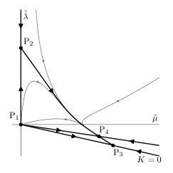
Figure 2: Renormalization group flow for the flat phase of crystalline membranes at one-loop order.

The lines $\mu_{0}=0$ and $B_{0}=0$ mark the boundaries of the overall region of stability for the elastic medium: $\mu_{0}\geq 0$, $B_{0}\geq 0$. Physically, the line $\mu_{0}=0$ has been proposed to be associated to fixed-connectivity fluid membranes [40], or possibly to generic fluid membranes [42]. A difficulty, however, is that the elastic energy associated with transverse waves is exactly zero for vanishing shear modulus, and higher-derivative terms of the form $(\partial^{2}u)^{2}$, neglected in the theory, could play a role [57]. The line $B_{0}=0$, instead, has a physical counterpart, for example, in two-dimensional twisted kagome lattices [56].

Coordinates of fixed points at one-loop order are reported in table 1 (for results at two-loops order see Ref. [49]).

	$\tilde{\lambda}_{*}$	$\tilde{\mu}_{*}$	$\eta_{*}$
P1	0	0	0
P2	$16\pi^{2}\varepsilon/d_{c}$	0	0
P3	$-48\pi^{2}\varepsilon/(d_{c}+20)$	$96\pi^{2}\varepsilon/(d_{c}+20)$	$10\varepsilon/(d_{c}+20)$
P4	$-32\pi^{2}\varepsilon/(d_{c}+24)$	$96\pi^{2}\varepsilon/(d_{c}+24)$	$12\varepsilon/(d_{c}+24)$

Table 1: Coordinates of fixed points and corresponding anomalous dimensions at leading order in the $\varepsilon$-expansion.

2.5 Bare renormalization group equations

To derive an alternative set of RG equations, we can introduce a cutoff scale $\Lambda$ and consider the Hamiltonian

$${\cal H}_{\Lambda}=\frac{1}{2}\int{\rm d}^{D}x\left[(\partial^{2}\mathbf{h})^{2}+\frac{c_{1}}{\Lambda^{2}}\left(\partial_{\alpha}\partial^{2}\mathbf{h}\right)^{2}+\frac{c_{2}}{\Lambda^{4}}\left(\partial^{2}\partial^{2}\mathbf{h}\right)^{2}+\lambda\Lambda^{\varepsilon}\left(u_{\alpha\alpha}\right)^{2}+2\mu\Lambda^{\varepsilon}u_{\alpha\beta}u_{\alpha\beta}+2\sigma\Lambda^{2}u_{\alpha\alpha}\right]~{}.$$ (15)

Eq. (15) is almost identical to the model discussed in Sec. 2.3, with three differences. The propagator of the $\mathbf{h}$ field, $G_{0}(\mathbf{k})=1/k^{4}$, is replaced here by a cutoff propagator $G_{0\Lambda}(\mathbf{k})=1/(k^{4}+c_{1}k^{6}/\Lambda^{2}+c_{2}k^{8}/\Lambda^{4})$. This is sufficient to regularize all ultraviolet divergences in perturbation theory, both in dimension four and in dimension $D=4-\varepsilon$ within the framework of the $\varepsilon$-expansion. A second difference is in the normalization of couplings: in Eq. (15) all dimensionful interactions are expressed by factorizing corresponding powers of the cutoff scale, in such way that the coefficients $c_{1}$, $c_{2}$, $\lambda$, $\mu$, and $\sigma$ are dimensionless. Finally, the ’tension’ term $\sigma u_{\alpha\alpha}$, which vanishes in dimensional regularization, is non-zero in general, and has been reintroduced in the expression of the Hamiltonian (effects of $\sigma$ have been discussed in Sec. 2.2).

To study scaling behavior, we can write bare RG equations [54] expressing the equivalence between changes of the cutoff and renormalizations of coupling constants:

$$\left[\frac{\partial}{\partial\ln\Lambda}\Big{|}_{\lambda,\mu}+\bar{\beta}_{\lambda}\frac{\partial}{\partial\lambda}\Big{|}_{\Lambda,\mu}+\bar{\beta}_{\mu}\frac{\partial}{\partial\mu}\Big{|}_{\Lambda,\lambda}+\left(\frac{n}{2}+\ell\right)\bar{\eta}\right]\langle h_{i_{1}}(\mathbf{x}_{1})..h_{i_{n}}(\mathbf{x}_{n})u_{\alpha_{1}}(\mathbf{x}^{\prime}_{1})..u_{\alpha_{\ell}}(\mathbf{x}^{\prime}_{\ell})\rangle=0~{},$$ (16)

or, for 1PI correlation functions with $n$ external $\mathbf{h}$ lines

$$\left[\frac{\partial}{\partial\ln\Lambda}\Big{|}_{\lambda,\mu}+\bar{\beta}_{\lambda}\frac{\partial}{\partial\lambda}\Big{|}_{\Lambda,\mu}+\bar{\beta}_{\mu}\frac{\partial}{\partial\mu}\Big{|}_{\Lambda,\lambda}-\left(\frac{n}{2}+\ell\right)\bar{\eta}\right]\Gamma^{(n,\ell)}_{i_{1}..i_{n}\alpha_{1}..\alpha_{\ell}}(\mathbf{k}_{1},..,\mathbf{k}_{n},\mathbf{k}^{\prime}_{1},..,\mathbf{k}^{\prime}_{\ell})=0~{}.$$ (17)

Eqs. (16) and (17) are a consequence of the perturbative renormalizability of the $\varepsilon$-expansion, which follows from power-counting arguments in analogy with other field theories [54]. As usual, the RG functions $\bar{\beta}_{\lambda}$, $\bar{\beta}_{\mu}$, and $\bar{\eta}$ cannot depend on $\Lambda$, because they are dimensionless and $\Lambda$ is the only scale in the problem. It follows that $\bar{\beta}_{\lambda}$, $\bar{\beta}_{\mu}$, and $\bar{\eta}$ depend only on the dimensionless bare couplings $\lambda$ and $\mu$, and, implicitly, on the specific form of regularization, expressed via the coefficients $c_{1}$ and $c_{2}$ (parameters which we choose to keep fixed as the cutoff is lowered).

In this setting, perturbative RG equations are closely analogue to Wilson’s exact renormalization group equations. The main difference is that in most formulations of Wilson’s RG the lowering of an UV cutoff is compensated by the flow of coupling constants exactly. Here, instead, after a change of $\Lambda$ and subsequent renormalizations, the physics is preserved up to small corrections which vanish roughly as $\Lambda^{-2}$ in the limit of $\Lambda$ large. In more detail, adapting an analogue result for the critical scalar field theory [54], we expect that 1PI correlation functions behave for large $\Lambda$ as

$$\mathbf{\Gamma}^{(n,\ell)}=k_{1\beta_{1}}..k_{n\beta_{n}}k^{\prime}_{1\gamma_{1}}..k^{\prime}_{\ell\gamma_{\ell}}\sum_{\begin{subarray}{c}m,p,q\geq 0\\ m+p+q=L-1+\frac{n}{2}+\ell\end{subarray}}\mathbf{\Gamma}_{Ls,mpq}^{(n,\ell)\beta_{1}..\beta_{n}\gamma_{1}..\gamma_{\ell}}\mu^{m}\lambda^{p}\left(\frac{\lambda\mu}{\lambda+2\mu}\right)^{q}\varepsilon^{s}~{},$$ (18)

where, schematically,

$$\mathbf{\Gamma}^{(n,\ell)}_{Ls,mpq}=\sum_{k=0}^{N(n,\ell,L,s)}\mathbf{\Gamma}^{(n,\ell)}_{Ls,mpq,k}(\ln\Lambda)^{k}+\Lambda^{-2}\times(\text{powers of }\ln\Lambda)+...$$ (19)

Perturbative renormalizability implies that the bare RG equations (16) and (17) are exact for the part which does not vanish in the limit $\Lambda\to\infty$ [54]. As a result, fixed points and anomalous dimensions of the perturbative renormalization group describe exactly the exponent of the leading scaling behavior, and only misses corrections due to strongly-irrelevant operators, separated by a large gap in the dilatation spectrum.

2.6 Comment on reflection positivity

Although we could not develop a detailed derivation, we expect that the membrane model discussed in this section is not reflection-positive. In the ultraviolet limit, where interactions can be neglected, the theory reduces to

$${\cal H}_{\rm UV}=\frac{1}{2}\int{\rm d}^{D}x\left[(\partial^{2}\mathbf{h})^{2}+(\lambda_{0}+\mu_{0})(\partial_{\alpha}u_{\alpha})^{2}+\mu_{0}\partial_{\alpha}u_{\beta}\partial_{\alpha}u_{\beta}\right]~{},$$ (20)

the combination of $d_{c}$ copies of a higher-derivative scalar theory and a Gaussian vector model. These non-interacting theories were analyzed in Refs. [58, 17, 19] and were shown to lack reflection positivity or, equivalently, unitarity in Minkowski space. We find it likely, therefore, that the also the full interacting model is not reflection-positive. A conclusive result requires, however, an analysis of the infrared region [59]. We leave this question to further investigations.

3 Gaussian-curvature interactions

In addition to the theory of elasticity, we discuss the relation between scale and conformal invariance in an alternative model, discussed in detail in Ref. [48] (see also Ref. [49]). The starting point in the derivation of this model is the observation that the Hamiltonian depends on the in-plane displacement fields $u_{\alpha}$ quadratically. As a result, integration over $u_{\alpha}$ can be computed analytically, and gives an effective interaction of a form already introduced in Eq. (8) [35, 38, 46]. In the case $D=2$, which is the dimension of interest physically, the geometrical structure of the effective interaction simplifies because, due to the presence of a single transverse direction, $P^{T}_{\alpha\beta}P^{T}_{\gamma\delta}=P^{T}_{\alpha\gamma}P^{T}_{\beta\delta}=P^{T}_{\alpha\delta}P^{T}_{\beta\gamma}$. As a result, the interaction becomes separable [44], and can be decoupled by introducing a scalar field via a Hubbard-Stratonovich transformation [48].

It follows that, for $D=2$, the physics of $\mathbf{h}$-field fluctuations can be captured by an alternative local field theory:

$${\cal H}=\int{\rm d}^{D}x\left[\frac{1}{2}(\partial^{2}\mathbf{h})^{2}+\frac{1}{2Y_{0}}(\partial^{2}\chi)^{2}+i\chi K\right]~{},$$ (21)

where $\chi$ is a scalar field mediating interactions and

$$K(\mathbf{x})=-\frac{1}{2}(\delta_{\alpha\beta}\partial^{2}-\partial_{\alpha}\partial_{\beta})(\partial_{\alpha}\mathbf{h}\cdot\partial_{\beta}\mathbf{h})=\frac{1}{2}[(\partial^{2}\mathbf{h}\cdot\partial^{2}\mathbf{h})-(\partial_{\alpha}\partial_{\beta}\mathbf{h}\cdot\partial_{\alpha}\partial_{\beta}\mathbf{h})]~{}.$$ (22)

As it can be shown, $K(\mathbf{x})$ is an approximate version of the Gaussian curvature of the membrane [38]. Eq. (21) thus expresses, qualitatively, a theory for membrane fluctuations with long-range interactions between Gaussian curvatures. In the following, Eq. (21) will be referred to as the ’Gaussian curvature interaction’, or ’GCI’ model.

The theory is controlled by a single coupling, the Young modulus $Y_{0}=4\mu_{0}(\lambda_{0}+\mu_{0})/(\lambda_{0}+2\mu_{0})$, which is proportional to both the shear coefficient $\mu_{0}$ and the two-dimensional bulk coefficient $\lambda_{0}+2\mu_{0}/D=\lambda_{0}+\mu_{0}$. Perturbative expansions can be computed from the Feynman rules in Fig. 3.

$$~{}\qquad\gamma(\mathbf{k}_{1},\mathbf{k}_{2},\mathbf{k}_{3})=k_{1}^{2}k_{2}^{2}-(\mathbf{k}_{1}\cdot\mathbf{k}_{2})^{2}=k_{2}^{2}k_{3}^{2}-(\mathbf{k}_{2}\cdot\mathbf{k}_{3})^{2}=k_{3}^{2}k_{1}^{2}-(\mathbf{k}_{3}\cdot\mathbf{k}_{1})^{2}$$

Figure 3: Feynman rules for the effective model. Solid and curly lines represent, respectively, propagators of the $\mathbf{h}$ and of the $\chi$ field.

As discussed in Ref. [48], the long-wavelength behavior of the theory can be studied by perturbative techniques within an $\varepsilon$-expansion near $D=4$, dimension in which the model is renormalizable.

Renormalization is particularly simple because, as an analysis of power counting shows, there are only two primitive divergences: the amplitude and the coupling constant renormalization [48, 46]. The vertex function, instead, is superficially UV-convergent. These properties follow directly from the special form of the vertex function $\gamma(\mathbf{k}_{1},\mathbf{k}_{2},\mathbf{k}_{3})$, which, in any 1PI diagram, allows to factorize two powers of each external momentum, reducing the degree of divergence. We note that a similar result emerges in Galileon theories, which can include terms of the same form of the interaction $i\chi K$ in Eq. (21). Also in these theories, vertex non-renormalization plays a crucial role [60].

Due to the considerations above, the renormalized action can be written as

$$\tilde{{\cal H}}=\int{\rm d}^{D}x\left[\frac{Z}{2}(\partial^{2}\mathbf{h})^{2}+\frac{1}{2Z_{Y}YM^{\varepsilon}}(\partial^{2}\chi)^{2}+i\chi K\right]~{},$$ (23)

where $M$ is an arbitrary scale, $Y$ is the dimensionless renormalized coupling, and $Z$, $Z_{Y}$ are divergent factors. After introduction of

$$\beta(Y)=\frac{\partial Y}{\partial\ln M}\Big{|}_{Y_{0}}~{},\qquad\eta(Y)=\frac{\partial\ln Z}{\partial\ln M}\Big{|}_{Y_{0}}~{},$$ (24)

the relations between bare and renormalized quantities

$$\mathbf{h}=\sqrt{Z}\tilde{\mathbf{h}}~{},\qquad\chi=Z^{-1}\tilde{\chi}~{},\qquad Y_{0}=M^{\varepsilon}\frac{Z_{Y}Y}{Z^{2}}$$ (25)

imply the RG equations

$$\left[\frac{\partial}{\partial\ln M}+\beta(Y)\frac{\partial}{\partial Y}+\left(\frac{n}{2}-\ell\right)\eta(Y)\right]\langle\tilde{h}_{i_{1}}(\mathbf{x}_{1})..\tilde{h}_{i_{n}}(\mathbf{x}_{n})\tilde{\chi}(\mathbf{x}^{\prime}_{1})..\tilde{\chi}(\mathbf{x}^{\prime}_{\ell})\rangle=0~{}.$$ (26)

For the renormalized 1PI functions with $n$ external $\mathbf{h}$ legs and $\ell$ external $\chi$ lines in momentum space, the corresponding RG relations read

$$\left[\frac{\partial}{\partial\ln M}+\beta(Y)\frac{\partial}{\partial Y}-\left(\frac{n}{2}-\ell\right)\eta(Y)\right]\tilde{\Gamma}^{(n,\ell)}=0~{}.$$ (27)

The $\beta$ function presents, in the $\varepsilon$-expansion, an infrared-stable interacting fixed point at $Y=Y_{*}$ with $Y_{*}={\rm O}(\varepsilon)$ [48, 49]. This fixed point controls the asymptotic infrared behavior. In particular, the propagator of the $\mathbf{h}$ field behaves as $G(\mathbf{k})=[\Gamma^{(2,0)}(\mathbf{k})]^{-1}\approx k^{-4+\eta_{*}}$, and the two-point function of the mediator field as $D(\mathbf{k})=[\Gamma^{(0,2)}(\mathbf{k})]^{-1}\approx k^{-D-2\eta_{*}}$. More generally $\Gamma^{(n,\ell)}$ behaves with overall momentum scale as $\Gamma^{(n,\ell)}\approx k^{D+\ell\eta_{*}+n(\varepsilon-\eta_{*})/2}$. The exponent has been calculated at two-loop order in Refs. [48, 49] and reads

$$\eta_{*}=\frac{2\varepsilon}{d_{c}+4}-\frac{d_{c}(2-d_{c})}{6(d_{c}+4)^{3}}\varepsilon^{2}+{\rm O}(\varepsilon^{3})~{}.$$ (28)

This exponent differs from anomalous dimensions of all fixed points in table 1 [49]. The GCI model, although equivalent to Eq. (6) for $D=2$, becomes a distinct theory in generic dimension, and provides a separate dimensional continuation to $D=4-\varepsilon$.

Finally, let us discuss the shift symmetries of the GCI model. The Hamiltonian density is invariant under the transformations $\mathbf{h}\to\mathbf{h}+\mathbf{A}+\mathbf{B}_{\alpha}x_{\alpha}$, where $\mathbf{A}$ and $\mathbf{B}_{\alpha}$ are vectors in $d_{c}$-dimensional space. The theory is also invariant under the shifts $\chi\to\chi+A^{\prime}+B^{\prime}_{\alpha}x_{\alpha}$, which change the energy density by a total derivative.

To conclude, we note that, the GCI model behaves in the UV as two copies of the biharmonic theory, which is not reflection-positive [58]. Thus, we find it likely that the full theory will also lack reflection positivity.

4 Energy-momentum tensor in scale-invariant and conformal field theories

Let us briefly discuss the relation between scale, conformal invariance, and the structure of the energy-momentum tensor. In any local Euclidean-invariant model, rotational symmetry implies the existence of an energy-momentum tensor $T_{\alpha\beta}$ which is symmetric and conserved [3, 2, 6]. As shown in Ref. [6], scale invariance requires that the trace is expressible as a total divergence,

$$T_{\alpha\alpha}=\partial_{\alpha}V_{\alpha}~{},$$ (29)

where $V_{\alpha}$ is a local ’virial current’ without explicit coordinate dependence. Conformal invariance requires instead a stronger condition [6]: that

$$T_{\alpha\alpha}=\partial_{\alpha}\partial_{\beta}L_{\alpha\beta}~{},$$ (30)

or, equivalently, that the virial current $V_{\alpha}$ can be expressed as $V_{\alpha}=J_{\alpha}+\partial_{\beta}L_{\alpha\beta}$, where $J_{\alpha}$ is a conserved current (with $\partial_{\alpha}J_{\alpha}=0$). In dimension $D=2$, two alternatives should be distinguished: if $L_{\alpha\beta}=\delta_{\alpha\beta}L$ the system displays invariance under the full infinite-dimensional group of local conformal maps. If, instead, $T_{\alpha\beta}=\partial_{\alpha}\partial_{\beta}L_{\alpha\beta}$ but $L_{\alpha\beta}$ is not expressible as $\delta_{\alpha\beta}L$ the theory is invariant under the global conformal group (it is ’Möbius invariant’), but not under the infinite Virasoro symmetry [50, 6].

A remark is that in scale- and conformally-invariant theories the relations (29) and (30) are usually not satisfied identically, but only up to operators which can be identified as generators of infinitesimal field redefinitions [28, 27, 30]. Examples of such operators are $\mathbf{E}\cdot\mathbf{h}$, $E_{\alpha}u_{\alpha}$, $\mathbf{E}\cdot\partial_{\beta}\mathbf{h}$ and $E_{\alpha}\partial_{\beta}u_{\alpha}$, where $\mathbf{E}(\mathbf{x})=\delta{\cal H}/\delta\mathbf{h}(\mathbf{x})$ and $E_{\alpha}(\mathbf{x})=\delta{\cal H}/\delta u_{\alpha}(\mathbf{x})$ are variational derivatives of the action, defining the equations of motion. When inserted in correlation functions, these operators produce contact terms and generate local changes of field variables which contribute to the transformation law of fields under scale and conformal maps [28, 27, 30]. Further, when referring to the operators $\mathbf{E}$ and $E_{\alpha}$, we will tell simply “equation of motion $E$” instead of “$E$ is the variational derivative of the action such that $E$ = 0 is the equation of motion”.

5 Scale vs. conformal invariance in linear elasticity theories

Before analyzing the complete theories, let us examine the membrane and the GCI model at the level of a non-interacting, free-field approximation.

For membrane theory, starting from the Hamiltonian defined in Eq. (9) and neglecting all interactions between the fields $\mathbf{h}$ and $u_{\alpha}$ we obtain:

$$H^{\prime\prime}=\frac{1}{2}\int{\rm d}^{D}x\left[(\partial^{2}\mathbf{h})^{2}+(\lambda_{0}+\mu_{0})(\partial_{\alpha}u_{\alpha})^{2}+\mu_{0}\partial_{\alpha}u_{\beta}\partial_{\alpha}u_{\beta}\right]~{}.$$ (31)

Fluctuations of $\mathbf{h}$ are thus described by the free bi-harmonic model $H^{(\mathbf{h})}=\int{\rm d}^{D}x(\partial^{2}\mathbf{h})^{2}/2$. It is a well-known result that this model is conformally-invariant in general dimension [50, 61]. An explicit calculation, in fact, shows that the theory admits a symmetric energy-momentum tensor with trace

$$T^{(\mathbf{h})}_{\alpha\alpha}=\frac{1}{2}(4-D)(\partial^{2}\mathbf{h})^{2}=\frac{1}{2}(4-D)\left[\mathbf{h}\cdot\partial^{2}\partial^{2}\mathbf{h}+\partial_{\alpha}\partial_{\beta}L_{\alpha\beta}\right]~{},$$ (32)

and $L_{\alpha\beta}=2(\partial_{\alpha}\mathbf{h}\cdot\partial_{\beta}\mathbf{h})-\delta_{\alpha\beta}(\partial_{\gamma}\mathbf{h}\cdot\partial_{\gamma}\mathbf{h})-\delta_{\alpha\beta}(\mathbf{h}\cdot\partial^{2}\mathbf{h})$. This form is consistent with that expected for a conformal theory [50]: the trace can be reduced to a total second derivative, up to the term $\mathbf{h}\cdot\partial^{2}\partial^{2}\mathbf{h}$, which vanishes with the equation of motion $\partial^{2}\partial^{2}\mathbf{h}=0$ and can be identified as the generator of local field rescaling. Since $L_{\alpha\beta}\neq\delta_{\alpha\beta}L$, the biharmonic theory in dimension $D=2$ is invariant under the global conformal group but not under the infinite Virasoro symmetry [50].

The theory for $u_{\alpha}$ fluctuations,

$$H^{(u)}=\frac{1}{2}\int{\rm d}^{D}x[(\lambda_{0}+\mu_{0})(\partial_{\alpha}u_{\alpha})^{2}+\mu_{0}\partial_{\alpha}u_{\beta}\partial_{\alpha}u_{\beta}]$$ (33)

is the well-known theory of linear isotropic elastic media. As it was shown in Refs. [17, 19], this model provides a physical realization of a scale-invariant but nonconformal field theory.

The lack of conformal invariance can be seen by showing that $u_{\alpha}$ cannot be a primary field nor a descendant [19]. That $u_{\alpha}$ is not primary follows from the fact that its two-point function is inconsistent with constraints imposed by conformal invariance. Any primary vector field $y_{\alpha}$ of dimension $\Delta_{y}$ in a CFT, in fact, presents a propagator with a specific tensor structure [19, 2, 21]:

$$\langle y_{\alpha}(\mathbf{x})y_{\beta}(\mathbf{x}^{\prime})\rangle=\frac{A}{|\mathbf{x}-\mathbf{x}^{\prime}|^{2\Delta_{y}}}\left(\delta_{\alpha\beta}-2\frac{(x_{\alpha}-x^{\prime}_{\alpha})(x_{\beta}-x^{\prime}_{\beta})}{|\mathbf{x}-\mathbf{x}^{\prime}|^{2}}\right)$$ (34)

in real space and

$$\langle y_{\alpha}(\mathbf{k})y_{\beta}(-\mathbf{k})\rangle=\frac{A^{\prime}}{k^{D-2\Delta_{y}}}\left(\delta_{\alpha\beta}+\frac{(D-2\Delta_{y})}{(\Delta_{y}-1)}\frac{k_{\alpha}k_{\beta}}{k^{2}}\right)$$ (35)

in momentum space. Explicit calculation of the propagator of $u_{\alpha}$, which has dimension $\Delta_{u}=(D-2)/2$, shows that its two-point function is inconsistent with Eq. (35), unless elastic constants are tuned in such way that $D\lambda_{0}+(D+4)\mu_{0}=0$. That $u_{\alpha}$ is not descendant follows from a simple dimensional analysis: for $D\geq 2$, $u_{\alpha}$ is the field with lowest possible dimension, and there exists no candidate operator with dimension $\{u_{\alpha}\}-1$ of which $u_{\alpha}$ could be a derivative. The conclusion is therefore that the theory is scale invariant but lacks conformal symmetry [19].

In $D=2$, the field dimension becomes $\Delta_{u}=0$, and the propagator behaves as $\ln|\mathbf{x}-\mathbf{x}^{\prime}|$, but it can still be shown that the theory lacks conformal invariance [17].

These results are confirmed by an inspection of the energy-momentum tensor: the theory admits an improved symmetric energy-momentum tensor $T_{\alpha\beta}$ with trace

$$T_{\alpha\alpha}=\partial_{\alpha}V_{\alpha}~{},\qquad V_{\alpha}=\frac{1}{2}(D\lambda_{0}+(D+2)\mu_{0})u_{\alpha}\partial_{\gamma}u_{\gamma}-\frac{1}{2}(D-2)\mu_{0}u_{\gamma}\partial_{\alpha}u_{\gamma}-\mu_{0}u_{\gamma}\partial_{\gamma}u_{\alpha}~{},$$ (36)

up to terms which vanish with the equations of motion. For generic $\lambda_{0}$ and $\mu_{0}$, the virial current cannot be reduced to the form $V_{\alpha}=j_{\alpha}+\partial_{\beta}L_{\alpha\beta}$, with $\partial_{\alpha}j_{\alpha}=0$, implying the absence of conformal invariance.

Conformal symmetry is only recovered in special cases. When $D\lambda_{0}+(D+4)\mu_{0}=0$, the virial current reduces to the form $V_{\alpha}=\partial_{\beta}L_{\alpha\beta}$, and the theory becomes conformal with $u_{\alpha}(\mathbf{x})$ as a primary field. The corresponding model is unphysical as an elasticity theory, being outside of the stability region $\mu_{0}\geq 0$, $B_{0}=\lambda_{0}+2\mu_{0}/D\geq 0$, but it is relevant for gauge-fixed electrodynamics [19].

For $\lambda_{0}+\mu_{0}=0$ another, ’twisted’, form of conformal invariance appears. In this case, the symmetry of the theory is enhanced from O$(D)$ to O$(D)\times$O$(D)$, and we can choose to regard $u_{\alpha}$ as a set of scalar fields rather than a vector field [17, 21]. The Hamiltonian is identical to $D$ copies of free scalar field theory, and is, therefore, conformal. The possibility to consider $u_{\alpha}$ as a collection of scalars, however, is destroyed in the full membrane model, which breaks O$(D)\times$O$(D)$ symmetry even for $\lambda_{0}+\mu_{0}=0$.

As mentioned in Sec. 2.4, a form of embedding-space conformal invariance appears for zero bulk modulus $B_{0}=\lambda_{0}+2\mu_{0}/D=0$. In this case, Eq. (33) is invariant under the shift of displacement fields $u_{\alpha}\to u_{\alpha}+\tau_{\alpha}$, where $\tau_{\alpha}$ is a conformal Killing vector with $\partial_{\alpha}\tau_{\beta}+\partial_{\beta}\tau_{\alpha}=2\delta_{\alpha\beta}(\partial_{\gamma}\tau_{\gamma})/D$ [42, 56]. This symmetry differs from the usual definition of conformal invariance in CFT, because transformations act as shifts of the fields and not as shifts of the coordinates $\mathbf{x}$.

Finally, Ref. [50] showed that in two dimensions the elasticity model for any choice of $\lambda_{0}$ and $\mu_{0}$ presents a hidden conformal symmetry which emerges when displacement fields are represented as gradients of scalar potentials: $u_{\alpha}=\partial_{\alpha}\phi+\epsilon_{\alpha\beta}\partial_{\beta}\omega$, where $\phi$ and $\omega$ are respectively a scalar and a pseudoscalar field. This representation maps Eq. (33) to two copies of the biharmonic theory, which is conformal in general dimension.

The GCI model defined in Eq. (21), similarly, reduces to two decoupled biharmonic theories in the non-interacting limit $Y_{0}\to 0$.

6 Scale vs. conformal invariance in membrane theory

6.1 Inconsistency between vector two-point function and conformal selection rules

To analyze whether conformal invariance holds in membrane theory, let us examine the two-point function $D_{\alpha\beta}(\mathbf{k})$ of the vector field $u_{\alpha}$ in momentum space. If we choose a renormalization scale $M\simeq|\mathbf{k}|$ of the order of the magnitude of a given momentum of interest, the renormalized propagator $\tilde{D}_{\alpha\beta}(\mathbf{k})=Z^{-2}D_{\alpha\beta}(\mathbf{k})$ is accurately captured by renormalized perturbation theory and, thus, for $\varepsilon$ small, can be approximated by the corresponding tree-level contribution. After calculation at scales $|\mathbf{k}|\simeq M$, the result can be rescaled to any wavelength via scaling relations. We thus deduce that the correlation function at an arbitrary $\mathbf{k}$ in the infrared region takes approximately the form

$$\tilde{D}_{\alpha\beta}(\mathbf{k})\simeq\frac{1}{M^{2\eta_{*}}k^{6-D-2\eta_{*}}}\left[\frac{P^{L}_{\alpha\beta}(\mathbf{k})}{\tilde{\lambda}_{*}+2\tilde{\mu}_{*}}+\frac{P^{T}_{\alpha\beta}(\mathbf{k})}{\tilde{\mu}_{*}}\right]~{},$$ (37)

where $P^{L}_{\alpha\beta}=k_{\alpha}k_{\beta}/k^{2}$ and $P^{T}_{\alpha\beta}=\delta_{\alpha\beta}-k_{\alpha}k_{\beta}/k^{2}$ are longitudinal and transverse projectors. In particular, the fixed point values of the renormalized couplings can be used to estimate, at the leading order in the $\varepsilon$-expansion, the tensor structure of $D_{\alpha\beta}(\mathbf{k})$.

We can now compare Eq. (37) with Eq. (35), the special form of the two-point function of a primary vector field. Near $D=4$, the scaling dimension of $u_{\alpha}$ is $\Delta_{u}=(1+\eta_{*}-\varepsilon)\simeq 1$ and thus, Eq. (35) implies that a vector consistent with conformal symmetry should have a two-point function which is almost purely longitudinal. In contrast, taking the O$(\varepsilon)$ values of the couplings at the fixed point P₄, $\tilde{\mu}_{*}=96\pi^{2}\varepsilon/(d_{c}+24)$, $\tilde{\lambda}_{*}=-\tilde{\mu}_{*}/3$, we see that in $\tilde{D}_{\alpha\beta}(\mathbf{k})$ longitudinal and transverse components have the same order of magnitude. This consideration, in analogy with Ref. [19] shows that $u_{\alpha}$ cannot be a conformal primary field.

6.2 Analysis of the virial current

For an alternative analysis, let us consider the structure of the energy-momentum tensor. An explicit calculation gives

$$\begin{split}T_{\alpha\beta}&=-\frac{1}{2}\delta_{\alpha\beta}\left[(\partial^{2}\mathbf{h})^{2}+\lambda_{0}(u_{\gamma\gamma})^{2}+2\mu_{0}u_{\gamma\delta}u_{\gamma\delta}\right]+2\partial_{\alpha}\partial_{\beta}\mathbf{h}\cdot\partial^{2}\mathbf{h}-\partial_{\alpha}\mathbf{h}\cdot\partial_{\beta}\partial^{2}\mathbf{h}-\partial_{\beta}\mathbf{h}\cdot\partial_{\alpha}\partial^{2}\mathbf{h}\\ &+\frac{1}{D-1}\left[\delta_{\alpha\beta}\partial_{\gamma}\mathbf{h}\cdot\partial_{\gamma}\partial^{2}\mathbf{h}+\delta_{\alpha\beta}\partial_{\gamma}\partial_{\delta}\mathbf{h}\cdot\partial_{\gamma}\partial_{\delta}\mathbf{h}+(D-2)\partial_{\gamma}\mathbf{h}\cdot\partial_{\alpha}\partial_{\beta}\partial_{\gamma}\mathbf{h}-D\partial_{\alpha}\partial_{\gamma}\mathbf{h}\cdot\partial_{\beta}\partial_{\gamma}\mathbf{h}\right]\\ &+2\lambda_{0}u_{\gamma\gamma}u_{\alpha\beta}+4\mu_{0}u_{\alpha\gamma}u_{\beta\gamma}-\frac{1}{2}(E_{\alpha}u_{\beta}+E_{\beta}u_{\alpha})+\lambda_{0}\partial_{\gamma}\left[(\delta_{\alpha\beta}u_{\gamma}-\delta_{\beta\gamma}u_{\alpha}-\delta_{\alpha\gamma}u_{\beta})u_{\delta\delta}\right]\\ &+2\mu_{0}\partial_{\gamma}\left[u_{\gamma}u_{\alpha\beta}-u_{\alpha}u_{\beta\gamma}-u_{\beta}u_{\alpha\gamma}\right]~{},\end{split}$$ (38)

which is symmetric and locally conserved. The conservation law for $T_{\alpha\beta}$, in particular, reads

$$\partial_{\alpha}T_{\alpha\beta}=-\mathbf{E}\cdot\partial_{\beta}\mathbf{h}-E_{\alpha}\partial_{\beta}u_{\alpha}-\frac{1}{2}\partial_{\alpha}(E_{\beta}u_{\alpha}-E_{\alpha}u_{\beta})$$ (39)

where

$$\mathbf{E}=\frac{\delta{\cal H}}{\delta\mathbf{h}}=\partial^{2}\partial^{2}\mathbf{h}-\partial_{\alpha}(\lambda_{0}u_{\beta\beta}\partial_{\alpha}\mathbf{h}+2\mu_{0}u_{\alpha\beta}\partial_{\beta}\mathbf{h})~{},\qquad E_{\alpha}=\frac{\delta{\cal H}}{\delta u_{\alpha}}=-\lambda_{0}\partial_{\alpha}u_{\beta\beta}-2\mu_{0}\partial_{\beta}u_{\alpha\beta}~{},$$ (40)

are equations of motion of the $\mathbf{h}$ and the $u_{\alpha}$ field. In contrast with the free-field approximation discussed in Sec. 5, the theory at finite $\lambda_{0}$ and $\mu_{0}$ is neither conformal nor scale invariant. The reason is that coupling constants are dimensionful, with dimension $\{\lambda_{0}\}=\{\mu_{0}\}=\varepsilon$, and introduce a characteristic length in the problem. Dilatation symmetry emerges only asymptotically, in the infrared region, when the theory becomes controlled by a fixed point. Adapting a method which was widely used in other field theories [27, 28], we examine this region by expanding $T_{\alpha\alpha}$ on a basis of renormalized composite operators, $[(u_{\alpha\alpha})^{2}]$, $[u_{\alpha\beta}u_{\alpha\beta}]$, $[u_{\alpha}u_{\beta\beta}]$, and $[u_{\beta}u_{\alpha\beta}]$, defined by suitable subtractions in such way that, order by order in perturbation theory, their insertion into renormalized correlation functions is ultraviolet-finite (free of poles in $\varepsilon$ for $\varepsilon\to 0$).

Detailed derivations, illustrated in appendices A and B show that the relation between the bare fields $u_{\alpha\beta}$, $u_{\alpha\alpha}$, $(\partial^{2}\mathbf{h})^{2}$, $u_{\alpha}u_{\beta\beta}$, $u_{\beta}u_{\alpha\beta}$ and the corresponding renormalized operators is almost completely determined by the RG functions $\beta_{\lambda}$, $\beta_{\mu}$, $\eta$, and by amplitude and coupling constant renormalizations ($Z$, $G_{\lambda}$ and $G_{\mu}$) which can be calculated from correlation functions without operator insertions. In particular, we can obtain relations for two distinct types of operators. A first type is the group of composite fields $\mathcal{O}_{1}=(\partial^{2}\mathbf{h})^{2}/2+\lambda_{0}(u_{\alpha\alpha})^{2}+2\mu_{0}u_{\alpha\beta}u_{\alpha\beta}$, $\mathcal{O}_{2}=\lambda_{0}(u_{\alpha\alpha})^{2}/2$, $\mathcal{O}_{3}=\mu_{0}u_{\alpha\beta}u_{\alpha\beta}$, $\mathcal{O}_{4}=\partial^{2}u_{\alpha\alpha}$, $\mathcal{O}_{5}=\partial_{\alpha}\partial_{\beta}u_{\alpha\beta}$, $\mathcal{O}_{6}=u_{\alpha\alpha}$, which are invariant under all symmetries of the Hamiltonian. For these operators, the analysis is closely analogue to derivations in Ref. [27] (see appendix A): we can express, to all orders in perturbation theory, the scale-invariance breaking effects in $T_{\alpha\alpha}$ in terms of renormalized composite fields multiplied by RG functions.

A second type is constituted by the operators $u_{\alpha}u_{\beta\beta}$ and $u_{\beta}u_{\alpha\beta}$, which break the shift symmetry $u_{\alpha}\to u_{\alpha}+B_{\alpha}$ and the invariance under the approximate embedding-space rotations defined in Eq. (7). As shown in appendix B, their explicit renormalization relation reads (in a non-minimal scheme):

$$u_{\alpha}u_{\beta\beta}=\frac{M^{\varepsilon}(D\tilde{\lambda}+2\tilde{\mu})}{D\lambda_{0}+2\mu_{0}}[u_{\alpha}u_{\beta\beta}]+b_{1}\partial_{\alpha}[\partial_{\beta}\mathbf{h}\cdot\partial_{\beta}\mathbf{h}]+b_{2}\partial_{\beta}[\partial_{\alpha}\mathbf{h}\cdot\partial_{\beta}\mathbf{h}]+b_{3}\partial^{2}[u_{\alpha}]+b_{4}\partial_{\alpha}\partial_{\beta}[u_{\beta}]~{},$$ (41)

$$\begin{split}u_{\beta}u_{\alpha\beta}-\frac{1}{D}u_{\alpha}u_{\beta\beta}&=\frac{M^{\varepsilon}\tilde{\mu}}{\mu_{0}}\left\{[u_{\beta}u_{\alpha\beta}]-\frac{1}{D}[u_{\alpha}u_{\beta\beta}]\right\}\\ &+b^{\prime}_{1}\partial_{\alpha}[\partial_{\beta}\mathbf{h}\cdot\partial_{\beta}\mathbf{h}]+b^{\prime}_{2}\partial_{\beta}[\partial_{\alpha}\mathbf{h}\cdot\partial_{\beta}\mathbf{h}]+b^{\prime}_{3}\partial^{2}[u_{\alpha}]+b^{\prime}_{4}\partial_{\alpha}\partial_{\beta}[u_{\beta}]~{}.\end{split}$$ (42)

where $b_{k}$ and $b^{\prime}_{k}$, $k=1,..,4$ are ultraviolet divergent coefficients. These relations can be interpreted as ’non-renormalizations’, in the sense that the product of bare couplings with bare operators is equal to the product of renormalized couplings and renormalized operators. Eqs. (41) and (42) are much simpler than the general relations expected by symmetry and power counting: counterterms with the schematic form $u^{3}$ are absent and mixing of operators of the type $u(\partial\mathbf{h}\cdot\partial\mathbf{h})$ and $u\partial u$ is exactly determined in terms of the elementary renormalization constants $Z$, $G_{\lambda}$, and $G_{\mu}$. Although appendix B presents a more complete proof, the particular simplicity of the renormalization relations can be directly understood from the structure of Feynman rules: in almost any diagram, we can factorize a power of the momentum of each external line. Diagrammatic corrections, therefore, tend to be shift-symmetric even if the inserted operators $u_{\alpha}u_{\beta\beta}$ and $u_{\beta}u_{\alpha\alpha}$ are not. This, in particular, protects the ’diagonal’ renormalization (the generation of counterterms proportional to the inserted composite fields $u_{\alpha}u_{\beta\beta}$ and $u_{\beta}u_{\alpha\beta}$) and implies the simple normalization formulas (41) and (42). A similar non-renormalization property associated with shift invariance occurs in Galileon theories [60].

For the following analysis, it is also useful to note that the composite operator $E_{\alpha}h^{2}$ is not renormalized: $[E_{\alpha}h^{2}]=E_{\alpha}h^{2}$. In fact, power counting shows that the product $(\mathbf{h}(\mathbf{x})\cdot\mathbf{h}(\mathbf{x}))$ at coincident points does not generate UV divergences. As a result $[h^{2}]=\tilde{\mathbf{h}}\cdot\tilde{\mathbf{h}}=Z^{-1}h^{2}$, where $Z$ is the field-amplitude renormalization. On the other hand, $E_{\alpha}(\mathbf{x}^{\prime})h^{2}(\mathbf{x}^{\prime})$ is a redundant operator which vanishes with equations of motion and acts as the infinitesimal generator of the field redefinition $u_{\beta}(\mathbf{x})\to u_{\beta}(\mathbf{x})-\epsilon\delta_{\alpha\beta}\delta(\mathbf{x}-\mathbf{x}^{\prime})h^{2}(\mathbf{x})$. Since $u_{\alpha}$ renormalizes as $\tilde{u}_{\alpha}=Z^{-1}u_{\alpha}$, insertion of $E_{\alpha}(\mathbf{x}^{\prime})h^{2}(\mathbf{x}^{\prime})$ can be equivalently represented as the generator of the infinitesimal transformation $\tilde{u}_{\alpha}(\mathbf{x})\to\tilde{u}_{\alpha}(\mathbf{x})-\epsilon\delta_{\alpha\beta}\delta(\mathbf{x}-\mathbf{x}^{\prime})[h^{2}(\mathbf{x})]$, which is finite and, thus, does not require subtractions.

Collecting results, we obtain the following equivalent expressions for the trace $T_{\alpha\alpha}$:

$$\begin{split}T_{\alpha\alpha}&=(\varepsilon-\eta)\left(\frac{1}{2}(\partial^{2}\mathbf{h})^{2}+\lambda_{0}(u_{\alpha\alpha})^{2}+\mu_{0}u_{\alpha\beta}u_{\alpha\beta}\right)-E_{\alpha}u_{\alpha}+\frac{1}{2}\beta_{\lambda}M^{\varepsilon}\left[(u_{\alpha\alpha})^{2}\right]+\beta_{\mu}M^{\varepsilon}[u_{\alpha\beta}u_{\alpha\beta}]\\ &+((D-2)\lambda_{0}+2\mu_{0})\partial_{\alpha}(u_{\alpha}u_{\beta\beta})-4\mu_{0}\partial_{\alpha}(u_{\beta}u_{\alpha\beta})+a_{1}\partial^{2}u_{\alpha\alpha}+a_{2}\partial_{\alpha}\partial_{\beta}u_{\alpha\beta}\\ &=-\frac{(\eta-\varepsilon)}{2}\mathbf{E}\cdot\mathbf{h}-(1+\eta-\varepsilon)E_{\alpha}u_{\alpha}+\frac{1}{2}\beta_{\lambda}M^{\varepsilon}[(u_{\alpha\alpha})^{2}]+\beta_{\mu}M^{\varepsilon}[u_{\alpha\beta}u_{\alpha\beta}]+\partial_{\alpha}V_{\alpha}~{},\end{split}$$ (43)

with

$$\begin{split}V_{\alpha}&=-\frac{1}{4}(\eta-\varepsilon)E_{\alpha}h^{2}+((2-\eta)\lambda_{0}+2\mu_{0})u_{\alpha}u_{\beta\beta}-2(2+\eta-\varepsilon)\mu_{0}u_{\beta}u_{\alpha\beta}\\ &+\frac{1}{2}(\varepsilon-\eta)\partial_{\beta}\left(-\delta_{\alpha\beta}(\mathbf{h}\cdot\partial^{2}\mathbf{h})+\frac{\lambda_{0}}{2}\delta_{\alpha\beta}h^{2}u_{\gamma\gamma}+\mu_{0}h^{2}u_{\alpha\beta}\right)+a_{1}\partial_{\alpha}u_{\beta\beta}+a_{2}\partial_{\beta}u_{\alpha\beta}\end{split}$$ (44)

or, after expansion in the basis of renormalized operators $[u_{\alpha}u_{\beta\beta}]$, $[u_{\beta}u_{\alpha\beta}]$,

$$\begin{split}V_{\alpha}&=-\frac{1}{4}(\eta-\varepsilon)E_{\alpha}h^{2}+((2-\eta)\tilde{\lambda}+2\tilde{\mu})M^{\varepsilon}[u_{\alpha}u_{\beta\beta}]-2(2+\eta-\varepsilon)\tilde{\mu}M^{\varepsilon}[u_{\beta}u_{\alpha\beta}]+\partial_{\beta}L_{\alpha\beta}~{},\\ L_{\alpha\beta}&=\frac{1}{2}(\varepsilon-\eta)\left[-\delta_{\alpha\beta}\mathbf{h}\cdot\partial^{2}\mathbf{h}+\frac{1}{2}\lambda_{0}\delta_{\alpha\beta}h^{2}u_{\gamma\gamma}+\mu_{0}h^{2}u_{\alpha\beta}\right]+b_{1}\delta_{\alpha\beta}(\partial_{\gamma}u_{\gamma})\\ &+b_{2}(\partial_{\alpha}u_{\beta}+\partial_{\beta}u_{\alpha})+b_{3}\delta_{\alpha\beta}(\partial_{\gamma}\mathbf{h}\cdot\partial_{\gamma}\mathbf{h})+b_{4}\partial_{\alpha}\mathbf{h}\cdot\partial_{\beta}\mathbf{h}~{}.\end{split}$$ (45)

In Eqs. (43), (44), and (45), $a_{1}$, $a_{2}$, and $b_{i}$, ($i=1,..,4$) are UV-divergent coefficients generated by renormalization.

In order to analyze scale and conformal invariance in the asymptotic infrared region, we assume that all renormalized operators remain finite when $\tilde{\lambda}$ and $\tilde{\mu}$ approach their fixed point values $\tilde{\lambda}\to\tilde{\lambda}_{*}$ and $\tilde{\mu}\to\tilde{\mu}_{*}$. Since $\beta_{\lambda}=\beta_{\mu}=0$ at the IR fixed point, the scale-invariance breaking terms $\beta_{\lambda}M^{\varepsilon}[(u_{\alpha\alpha})^{2}]/2+\beta_{\mu}M^{\varepsilon}[u_{\alpha\beta}u_{\alpha\beta}]$ can be dropped from the expression of $T_{\alpha\alpha}$ and the scaling symmetry of the theory, known from RG arguments, becomes manifest. In particular, we can define a dilatation current $S_{\alpha}=x_{\beta}T_{\alpha\beta}-V_{\alpha}$ [6] which is locally conserved and presents a conservation law

$$\partial_{\alpha}S_{\alpha}=-x_{\beta}\left(\mathbf{E}\cdot\partial_{\beta}\mathbf{h}+E_{\alpha}\partial_{\beta}u_{\alpha}\right)-\frac{(\eta_{*}-\varepsilon)}{2}\mathbf{E}\cdot\mathbf{h}-(1+\eta_{*}-\varepsilon)E_{\alpha}u_{\alpha}~{},$$ (46)

consistent with the form expected for fields of dimension $\Delta_{\mathbf{h}}=\{\mathbf{h}\}=(\eta_{*}-\varepsilon)/2$ and $\Delta_{u}=\{u_{\alpha}\}=(1+\eta_{*}-\varepsilon)$ [27, 28]. More generally it is possible to show that, for general $\tilde{\lambda}$ and $\tilde{\mu}$, the Ward identity generated by the dilatation current is equivalent to the RG equation (see appendix A), similarly to the case of scalar field theory [27].

The vanishing of $\beta$ functions, however, is not sufficient to imply the conformal invariance of the model due to the presence of the non-zero virial current $V_{\alpha}$. An algebraic analysis of terms in Eq. (44) shows that $V_{\alpha}$ cannot be written as the total derivative $V_{\alpha}=\partial_{\beta}l_{\alpha\beta}$ of a local operator $l_{\alpha\beta}$. This remains true even in the scale-invariant infrared limit because, as Eq. (45) shows, contributions proportional to $E_{\alpha}h^{2}$, $[u_{\alpha}u_{\beta\beta}]$, $[u_{\beta}u_{\alpha\beta}]$ do not vanish as $\tilde{\lambda}$ and $\tilde{\mu}$ approach their fixed point value. It follows that it is impossible to construct a conformal current with the form [6]

$$C_{\mu,\alpha}=(2x_{\mu}x_{\beta}-\delta_{\mu\beta}x^{2})T_{\alpha\beta}-2x_{\mu}V_{\alpha}+2l_{\mu\alpha}$$ (47)

and the conservation law

$$\partial_{\alpha}C_{\mu,\alpha}=-(2x_{\mu}x_{\beta}-\delta_{\mu\beta}x^{2})(\mathbf{E}\cdot\partial_{\beta}\mathbf{h}+E_{\gamma}\partial_{\beta}u_{\gamma})+2x_{\beta}(E_{\beta}u_{\mu}-E_{\mu}u_{\beta})-2x_{\mu}\left(\Delta_{\mathbf{h}}\mathbf{E}\cdot\mathbf{h}+\Delta_{u}E_{\alpha}u_{\alpha}\right)$$ (48)

expected for a scenario in which $\mathbf{h}$ and $u_{\alpha}$ are conformal primary fields.

It is also impossible to reduce $V_{\alpha}$ to the form $j_{\alpha}+\partial_{\beta}l_{\alpha\beta}$ where $j_{\alpha}$ is a conserved current. If $V_{\alpha}=j_{\alpha}+\partial_{\beta}l_{\alpha\beta}$ was true, the total derivative $\partial_{\alpha}V_{\alpha}$ should reduce to a combination $\mathcal{O}_{\rm red}+\partial_{\alpha}\partial_{\beta}l_{\alpha\beta}$, where $\mathcal{O}_{\rm red}$ is a redundant operator, removable by field redefinition. Working within dimensional regularization, we can assume that the $\mathcal{O}_{\rm red}$ has the form $E_{\alpha}\chi_{\alpha}+\mathbf{E}\cdot\mathbf{F}$, where $\chi_{\alpha}$ and $\mathbf{F}$ are local functionals of the field, and we can neglect contributions arising from the Jacobian of the transformation. The only candidates for $\mathcal{O}_{\rm red}$ with power-counting dimension $4$ near $D=4$ are then linear combinations of the form $f_{1}(h^{2})\mathbf{E}\cdot\mathbf{h}+f_{2}(h^{2})E_{\alpha}u_{\alpha}+f_{3}(h^{2})E_{\alpha}(\mathbf{h}\cdot\partial_{\alpha}\mathbf{h})$, where $f_{1}(h^{2})$, $f_{2}(h^{2})$, $f_{3}(h^{2})$ are functions of $h^{2}$. We checked by explicit calculation that $\partial_{\alpha}V_{\alpha}$ cannot be reduced to such a combination up to a total second derivative $\partial_{\alpha}\partial_{\beta}l_{\alpha\beta}$.

We can thus conclude that the form of the virial current is inconsistent with the structure expected in a conformal theory. Therefore, the theory must exhibit only scale invariance and not the enhanced conformal symmetry. This confirms the result expected from the inconsistency of conformal selection rules illustrated in Sec. 6.1 and also excludes the possibility that conformal invariance is realized in a more general way, with a transformation law of $u_{\alpha}$ differing from that of a primary field.

As a remark, we note that the arguments above rely essentially on the ’non-renormalization’ relations (41), (42), which allowed to control contributions to the energy-momentum tensor in the limit $(\tilde{\lambda},\tilde{\mu})\to(\tilde{\lambda}_{*},\tilde{\mu}_{*})$ via subtracted fields. In fact, when $\tilde{\lambda}$ and $\tilde{\mu}$ approach their fixed point values, the bare couplings $\lambda_{0}$ and $\mu_{0}$ diverge. We assume, instead, that subtracted quantities remain finite. Differently from the scale-invariance breaking terms, which vanished as $\beta_{\lambda}$, $\beta_{\mu}\to 0$, there is no analogue cancellation of conformal-breaking terms at the fixed point.

To conclude, we notice that, due to the use of dimensional regularization, the role of the ’tension’ counterterm $\sigma u_{\alpha\alpha}$ described in Sec. 2.2 remained hidden. The symmetric energy-momentum tensor corresponding to this term is proportional to $(\partial\mathbf{h})^{2}$ and thus, breaks the rotational invariance in the embedding space. The effects of these terms on the relation between scale and conformal invariance can be analyzed by generalizing the bare RG equations of Sec. 2.5 to composite operators.

6.3 Scaling dimension of the virial current

Having obtained that the membrane theory is not conformal, let us comment on the naturalness of having vector operators with dimension exactly equal to $D-1$. The absence of anomalous dimensionality is a direct consequence of the ’non-renormalization’ relations (41), (42). In fact, it can be seen by applying RG equations that both $u_{\alpha}u_{\beta\beta}$ and $u_{\beta}u_{\alpha\beta}$ scale at the IR fixed point with the same dimension and that the naive dimension $M^{\varepsilon}\{u_{\alpha}u_{\beta\beta}\}=D-1$ remains true in the long-wavelength region. This dimension can also be interpreted as the sum of the infrared dimensions of $u_{\alpha}$, which is $1+\eta_{*}-\varepsilon$ by the RG equations (13), and $u_{\alpha\beta}$ which, as shown in appendix A has dimension $2-\eta_{*}$. The ’non-renormalization’ properties imply that the combination of $u_{\alpha}$ and $u_{\alpha\beta}$ into a single operator does not generate any new divergences and, therefore, anomalous dimensions.

The existence of non-conserved currents with dimension exactly $D-1$ can thus be traced to the shift-symmetries of the model, which are responsible for the absence of renormalizations.

7 Symmetry argument for the absence of conformal invariance

The derivation in Sec. 6 suggests an important role of the shift symmetries of the model. In fact, an argument for the absence of conformal invariance can be directly deduced by considering the structure of the symmetries. The Hamiltonian of membrane theory is invariant under translations and rotations of the internal coordinates $\mathbf{x}$ and under embedding-space translations and rotations, which are realized as shifts of the $u_{\alpha}$ and $\mathbf{h}$ fields. The corresponding generators, written as operators acting on functionals of $\mathbf{h}$ and $u_{\alpha}$, can be written as

$$P_{\alpha}=-i\int{\rm d}^{D}x\left[\partial_{\alpha}\mathbf{h}\cdot\frac{\delta}{\delta\mathbf{h}}+\partial_{\alpha}u_{\beta}\frac{\delta}{\delta u_{\beta}}\right]~{},$$ (49)

$$J_{\alpha\beta}=i\int{\rm d}^{D}x\left[(x_{\alpha}\partial_{\beta}\mathbf{h}-x_{\beta}\partial_{\alpha}\mathbf{h})\cdot\frac{\delta}{\delta\mathbf{h}}+(x_{\alpha}\partial_{\beta}u_{\gamma}-x_{\beta}\partial_{\alpha}u_{\gamma})\frac{\delta}{\delta u_{\gamma}}+u_{\beta}\frac{\delta}{\delta u_{\alpha}}-u_{\alpha}\frac{\delta}{\delta u_{\beta}}\right]~{},$$ (50)

$$\mathbf{t}=-i\int{\rm d}^{D}x\frac{\delta}{\delta\mathbf{h}}~{},\qquad t_{\alpha}=-i\int{\rm d}^{D}x\frac{\delta}{\delta u_{\alpha}}~{},$$ (51)

$$\mathbf{R}_{\alpha}=i\int{\rm d}^{D}x\left[x_{\alpha}\frac{\delta}{\delta\mathbf{h}}-\mathbf{h}\frac{\delta}{\delta u_{\alpha}}\right]~{},\qquad R_{\alpha\beta}=i\int{\rm d}^{D}x\left[x_{\alpha}\frac{\delta}{\delta u_{\beta}}-x_{\beta}\frac{\delta}{\delta u_{\alpha}}\right]~{},$$ (52)

where bold symbols denote vectors in $d_{c}$-dimensional space. The generators $P_{\alpha}$ and $J_{\alpha\beta}$ of internal-space transformations satisfy the commutation relations of the Euclidean algebra: $[P_{\alpha},P_{\beta}]=0$, $[P_{\gamma},J_{\alpha\beta}]=i(\delta_{\alpha\gamma}P_{\beta}-\delta_{\beta\gamma}P_{\alpha})$, $[J_{\alpha\beta},J_{\gamma\delta}]=i(\delta_{\alpha\gamma}J_{\beta\delta}+\delta_{\beta\delta}J_{\alpha\gamma}-\delta_{\alpha\delta}J_{\beta\gamma}-\delta_{\beta\gamma}J_{\alpha\delta})$. For shift symmetries, we have, instead $[\mathbf{t}^{i},\mathbf{t}^{j}]=[\mathbf{t},t_{\alpha}]=[\mathbf{t},R_{\alpha\beta}]=[t_{\alpha},t_{\beta}]=[t_{\alpha},\mathbf{R}_{\beta}]=[t_{\alpha},R_{\beta\gamma}]=[\mathbf{R}_{\alpha},R_{\beta\gamma}]=[R_{\alpha\beta},R_{\gamma\delta}]=0$, where $\mathbf{t}^{i}$ denotes the $i$ component of the vector $\mathbf{t}$ in $d_{c}$-dimensional space. The only nonzero commutators between the embedding-space generators are $[\mathbf{t}^{i},\mathbf{R}^{j}_{\alpha}]=i\delta^{ij}t_{\alpha}$ and $[\mathbf{R}^{i}_{\alpha},\mathbf{R}^{j}_{\beta}]=i\delta^{ij}R_{\alpha\beta}$. Mixed commutators between shift generators and internal-space transformations have a simple form: in the commutation with $J_{\alpha\beta}$, the generator $\mathbf{t}$, which has no internal-space index, transforms as a scalar, $t_{\alpha}$ and $\mathbf{R}_{\alpha}$ as vectors, and $R_{\alpha\beta}$ as a second-rank tensor. Commutators between internal translations and shifts read $[P_{\alpha},\mathbf{t}]=[P_{\alpha},t_{\beta}]=0$, $[P_{\alpha},\mathbf{R}_{\beta}]=-i\delta_{\alpha\beta}\mathbf{t}$, $[P_{\gamma},R_{\alpha\beta}]=-i(\delta_{\gamma\alpha}t_{\beta}-\delta_{\gamma\beta}t_{\alpha})$.

At the IR fixed point, the theory acquires an additional dilatation symmetry. We can represent the corresponding generator as

$$D=-i\int{\rm d}^{D}x\left[\left(x_{\alpha}\partial_{\alpha}\mathbf{h}+\Delta_{\mathbf{h}}\mathbf{h}\right)\cdot\frac{\delta}{\delta\mathbf{h}}+\left(x_{\alpha}\partial_{\alpha}u_{\beta}+\Delta_{u}u_{\beta}\right)\frac{\delta}{\delta u_{\beta}}\right]~{},$$ (53)

where $\Delta_{\mathbf{h}}$ and $\Delta_{u}$ define the scaling dimension of fields. An analysis of the commutation relations between $D$ and the generators (49)–(53) shows that the algebra is not closed for general values of $\Delta_{\mathbf{h}}$ and $\Delta_{u}$. All commutators are linear combinations of generators a part from one:

$$[D,\mathbf{R}_{\alpha}]=\int{\rm d}^{D}x\left[(\Delta_{u}-\Delta_{\mathbf{h}})\mathbf{h}\frac{\delta}{\delta u_{\alpha}}-(\Delta_{\mathbf{h}}+1)x_{\alpha}\frac{\delta}{\delta\mathbf{h}}\right]~{},$$ (54)

which is not an element of the algebra. The only way to close the symmetry group without adding new generators is to assume that the field dimensions $\Delta_{u}$ and $\Delta_{\mathbf{h}}$ are related by $\Delta_{u}=2\Delta_{\mathbf{h}}+1$, in such way that $[D,\mathbf{R}_{\alpha}]=i(\Delta_{\mathbf{h}}+1)\mathbf{R}_{\alpha}$. This relation, in fact, is satisfied: it is exactly equivalent to the rotational Ward identity for scaling exponents [40, 42, 44] which, in the RG language, arises from the link between $\mathbf{h}$ and $u_{\alpha}$ amplitudes in the renormalization relations $\mathbf{h}=\sqrt{Z}\tilde{\mathbf{h}}$ and $u_{\alpha}=Z\tilde{u}_{\alpha}$. In a more conventional notation, $\Delta_{\mathbf{h}}$ and $\Delta_{u}$ are parametrized by a single anomalous dimension as $\Delta_{\mathbf{h}}=(\eta_{*}-\varepsilon)/2$ and $\Delta_{u}=1+\eta_{*}-\varepsilon$.

After fixing scaling dimensions as $\Delta_{\mathbf{h}}=\Delta$ and $\Delta_{u}=2\Delta+1$, let us suppose that the theory is conformal and that $\mathbf{h}$ and $u_{\alpha}$ are both primary fields. In this case the symmetry group would contain additional special conformal generators whose action can be represented as

$$\begin{split}K_{\alpha}&=-i\int{\rm d}^{D}x\Big{\{}\left[(2x_{\alpha}x_{\beta}-\delta_{\alpha\beta}x^{2})\partial_{\beta}\mathbf{h}+2\Delta x_{\alpha}\mathbf{h}\right]\cdot\frac{\delta}{\delta\mathbf{h}}\\ &+\left[(2x_{\alpha}x_{\beta}-\delta_{\alpha\beta}x^{2})\partial_{\beta}u_{\gamma}+2(2\Delta+1)x_{\alpha}u_{\gamma}\right]\frac{\delta}{\delta u_{\gamma}}+2(\delta_{\alpha\gamma}x_{\beta}-\delta_{\alpha\beta}x_{\gamma})u_{\beta}\frac{\delta}{\delta u_{\gamma}}\Big{\}}~{}.\end{split}$$ (55)

The introduction of $K_{\alpha}$, however, breaks the closure of the algebra. In particular the commutator

$$[K_{\alpha},\mathbf{t}]=2\Delta\int{\rm d}^{D}x~{}x_{\alpha}\frac{\delta}{\delta\mathbf{h}}$$ (56)

requires the introduction of a new generator

$$\mathbf{t}^{\prime}_{\alpha}=-i\int{\rm d}^{D}x~{}x_{\alpha}\frac{\delta}{\delta\mathbf{h}}~{}.$$ (57)

In turn, $[K_{\alpha},\mathbf{t}^{\prime}_{\beta}]$ requires to add a symmetry under

$$\mathbf{t}^{\prime\prime}_{\alpha\beta}=-i\int{\rm d}^{D}x~{}\left[2(1+\Delta)x_{\alpha}x_{\beta}-\delta_{\alpha\beta}x^{2}\right]\cdot\frac{\delta}{\delta\mathbf{h}}~{}.$$ (58)

For general anomalous dimensionality $\Delta$ the process can be iterated to obtain new shift symmetries. On physical grounds, however, we do not expect these symmetries to hold: shifting $\mathbf{h}\to\mathbf{h}+\mathbf{B}_{\alpha}x_{\alpha}$ without a compensating shift of $u_{\alpha}$ is not a symmetry of the Hamiltonian and we do not see reasons why it should emerge in the IR.

This argument indicates, consistently with the analysis in Sec. 6, that $\mathbf{h}$ can not be interpreted as the primary fields of a conformal field theory.

8 ’Gaussian curvature interaction’ model: scale without conformal invariance

Differently from elasticity theory, the GCI model is exactly conformal in the Gaussian approximation, and therefore, in the ultraviolet region. In fact, the Hamiltonian (21) reduces in the weak-coupling limit $Y_{0}\to 0$ to two copies of the biharmonic theory, which is exactly scale and conformal invariant [61, 50]. In this section we show that, instead, conformal symmetry is broken in the infrared region: the IR fixed point theory is only dilatation-invariant.

With calculations illustrated in appendix C and some further algebraic steps, it can be shown that the model admits a symmetric energy-momentum tensor $T_{\alpha\beta}$ with trace

$$\begin{split}T_{\alpha\alpha}&=-\frac{(\eta-\varepsilon)}{2}\mathbf{E}\cdot\mathbf{h}+\eta E\chi-\frac{\beta(Y)}{2Y^{2}}M^{-\varepsilon}[(\partial^{2}\chi)^{2}]+\partial_{\alpha}V_{\alpha}\end{split}$$ (59)

where

$$\mathbf{E}=\partial^{2}\partial^{2}\mathbf{h}+i(\partial^{2}\chi\partial^{2}\mathbf{h}-\partial_{\alpha}\partial_{\beta}\chi\partial_{\alpha}\partial_{\beta}\mathbf{h})~{},\qquad E=\frac{1}{Y_{0}}\partial^{2}\partial^{2}\chi+iK$$ (60)

are, respectively, the equations of motion of the $\mathbf{h}$ and the $\chi$ field, and $[(\partial^{2}\chi)^{2}]$ denotes the renormalized insertion of $(\partial^{2}\chi)^{2}$. The expression for $T_{\alpha\alpha}$ includes a non-zero ’virial current’

$$\begin{split}V_{\alpha}&=-\frac{i}{2}\big{\{}(D-3+2\eta)\partial_{\alpha}\chi(\partial_{\beta}\mathbf{h}\cdot\partial_{\beta}\mathbf{h})+2(1-\eta)\partial_{\beta}\chi(\partial_{\beta}\mathbf{h}\cdot\partial_{\alpha}\mathbf{h})\big{\}}+\partial_{\beta}L_{\alpha\beta}~{},\end{split}$$ (61)

where $L_{\alpha\beta}$ is a local tensor field.

At the IR fixed point $Y=Y_{*}$, assuming that the renormalized operator $[(\partial^{2}\chi)^{2}]$ remains finite, the term $-\beta(Y)M^{-\varepsilon}[(\partial^{2}\chi)^{2}]/(2Y^{2})$ becomes zero due to the vanishing of the $\beta$-function $\beta(Y_{*})=0$. We can thus introduce a dilatation current $S_{\alpha}=x_{\beta}T_{\alpha\beta}-V_{\alpha}$ which is locally conserved:

$$\partial_{\alpha}S_{\alpha}=-x_{\beta}(\mathbf{E}\cdot\partial_{\beta}\mathbf{h}+E\partial_{\beta}\chi)-\frac{(\eta_{*}-\varepsilon)}{2}\mathbf{E}\cdot\mathbf{h}+\eta_{*}E\chi~{}.$$ (62)

Whether the scaling symmetry is enhanced to the full conformal invariance depends on the structure of the virial current. It is useful, therefore, to examine insertions of the composite field $P_{\mu,\alpha\beta}=\partial_{\mu}\chi(\partial_{\alpha}\mathbf{h}\cdot\partial_{\beta}\mathbf{h})$, an elementary building block from which the nontrivial terms in Eq. (61) can be constructed. The renormalization of $P_{\mu,\alpha\beta}$ has a particularly simple form. In fact, let us consider an arbitrary diagram $\gamma$ for a 1PI correlation function with $n$ external $\mathbf{h}$ lines, $\ell$ external $\chi$ lines, and one insertion of $P_{\mu,\alpha\beta}$. The diagram can be of one of the three types illustrated in Fig. 4: in diagrams of the groups (a) and (b) one of the elementary fields contained in the composite operator is directly connected with external lines, while in diagrams of type (c) all inserted lines enter as loop propagators.

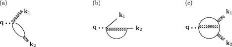
Figure 4: Examples of 1PI diagrams of type (a), (b), and (c).

The Feynman rules of the theory imply that the degree of superficial divergence [54] is

$$\delta(\gamma)=3+DL-4I_{h}-4I_{\chi}+4v-2n-2\ell+a_{\gamma}~{},$$ (63)

where $I_{\mathbf{h}}$ and $I_{\chi}$ denote the number of internal $\mathbf{h}$ and $\chi$ propagators, $v$ the number of vertices, and $L$ the number of loops. The coefficient $a_{\gamma}$ is $a_{\gamma}=1$ for diagrams of type (a) and (b) and $a_{\gamma}=0$ for type (c). Using the topological relations $L=3+2v-I_{\mathbf{h}}-I_{\chi}-n-\ell$, $2I_{\mathbf{h}}+n=2v+2$, and $2I_{\chi}+\ell=v+1$, we see that the degree of divergence in the $\varepsilon$ expansion is

$$\delta(\gamma)=3-2n-2\ell+a_{\gamma}~{}.$$ (64)

It follows that the only counterterms needed for the renormalization of $P_{\mu,\alpha\beta}$ have the schematic form $\partial^{3}\chi$, $\partial\chi\partial^{2}\chi$, $\partial\mathbf{h}\cdot\partial^{2}\mathbf{h}$. These composite operators can always be represented as total derivatives (see Eq. (90)).

We can conclude that insertions of the composite fields $\partial_{\alpha}\chi(\partial_{\beta}\mathbf{h}\cdot\partial_{\beta}\mathbf{h})$ and $\partial_{\beta}\chi(\partial_{\alpha}\mathbf{h}\cdot\partial_{\beta}\mathbf{h})$, which contribute to the virial current, are finite up to total-derivative counterterms. Therefore, the “bulk” of the virial current is unrenormalized: we can set $\partial_{\alpha}\chi_{\beta}(\partial_{\beta}\mathbf{h}\cdot\partial_{\beta}\mathbf{h})=[\partial_{\alpha}\chi_{\beta}(\partial_{\beta}\mathbf{h}\cdot\partial_{\beta}\mathbf{h})]$ and $\partial_{\beta}\chi(\partial_{\alpha}\mathbf{h}\cdot\partial_{\beta}\mathbf{h})=[\partial_{\beta}\chi(\partial_{\alpha}\mathbf{h}\cdot\partial_{\beta}\mathbf{h})]$, up to gradients of the form $\partial_{\beta}l_{\alpha\beta}$ which do not affect the relation between scale and conformal invariance [6].

Let us check that $V_{\alpha}$ cannot be reduced completely to the combination $V_{\alpha}=j_{\alpha}+\partial_{\beta}L^{\prime}_{\alpha\beta}$ of a conserved current $j_{\alpha}$ and a total derivative. If this was the case, $\partial_{\alpha}V_{\alpha}$ should reduce to the combination $\mathcal{O}_{\rm red}+\partial_{\alpha}\partial_{\beta}l_{\alpha\beta}$ of a redundant operator $\mathcal{O}_{\rm red}$ and a total second derivative. Within dimensional regularization, candidates for $\mathcal{O}_{\rm red}$ can be taken as linear combinations of operators proportional to the equations of motion $\mathbf{E}$ and $E$ and, in order to match the power-counting dimension of $\partial_{\alpha}V_{\alpha}$, must have the form $f_{1}(h^{2},\chi)(\mathbf{E}\cdot\mathbf{h})+f_{2}(h^{2},\chi)E$, where $f_{1}$ and $f_{2}$ are functions. We checked from the explicit expression $V_{\alpha}$ that it is impossible to rewrite $\partial_{\alpha}V_{\alpha}$ as a combination of this type up to a total second derivative $\partial_{\alpha}\partial_{\beta}l_{\alpha\beta}$. Since contributions to $V_{\alpha}$ do not renormalize, we expect that this result remains robust at the IR fixed point. We are lead to the conclusion that the GCI model exhibits scale without conformal invariance.

Let us, then, investigate the scaling properties of the operators composing $V_{\alpha}$. Since $P_{\mu,\alpha\beta}$ is not renormalized, it does not acquire anomalous exponents. Therefore the naive dimension $\{P_{\mu,\alpha\beta}\}=3+2\{\mathbf{h}\}+\{\chi\}=3+2(D-4)/2+0=D-1$ remains valid at the IR fixed point²¹. This scaling relation can also be understood in terms of the infrared dimensions of fields. The renormalization relations discussed in Sec. 3, $\mathbf{h}=\sqrt{Z}\mathbf{h}$, $\chi=Z^{-1}\tilde{\chi}$, imply that $\mathbf{h}$ and $\chi$ scale in the long-wavelength limit with dimensionalities $\{\mathbf{h}\}=(D-4+\eta)/2$ and $\{\chi\}=-\eta$. The absence of divergences in the insertion of $P_{\mu,\alpha\beta}$ implies that the naive relation $\{V_{\alpha}\}=3+2\{\mathbf{h}\}+\{\chi\}$ remains valid in the IR and, in fact, it can be seen that the anomalous exponent $\eta$ cancels out leaving an exact canonical dimension.

The absence of nontrivial anomalous dimensions can be traced, as in the case of membrane theory, to the shift symmetries of the model. These symmetries are manifested in momentum space as a special property of Feynman rules: for each external line connected to interaction vertices, it is always possible to factorize two powers of the corresponding momentum. The result is a suppression of the degree of UV divergence [48, 46], which, in the power counting formula (63) is expressed by the terms $-2n-2\ell$. This explains why candidates for the virial current, which must have dimension $D-1$, arise naturally.

9 Summary and conclusions

To summarize, we analyzed two models for the scaling behavior of fluctuations in crystalline membranes: a widely-studied effective field theory based on elasticity and an alternative model, involving only scalar fields, which describes long-range phonon-mediated interactions between local Gaussian curvatures. For both models, we argued that the infrared behavior is only scale-invariant: the asymptotic dilatation symmetry is not promoted to conformal invariance. An analysis of the energy-momentum tensor of the two theories reveals, in both cases, the presence of non-trivial virial currents which, despite being non-conserved, maintain a scaling dimension equal to $D-1$, without corrections from interactions. We traced the origin of this non-renormalization to the shift symmetries of the theory, which forbid the generation of several counterterms which would be allowed by a first power-counting analysis. These results suggest a mechanism to elude a general reasoning according to which non-conserved currents with dimension $D-1$ are unlikely at generic interacting fixed points and thus, that conformal invariance should be an almost inevitable consequence of scale invariance in presence of interactions. As a complementary analysis, in the case of the nonlinear elasticity theory of membranes, we present a simple argument, based only on the structure of symmetries, which suggests an inconsistency between conformal invariance and the invariance of the model under shifts. The results derived in this paper are not in contradiction with general theorems and derivations on the relation between scale and conformal symmetries for two reasons. First, we expect that the models investigated in this work are not reflection-positive. Secondly, we studied fixed points in $D=4-\varepsilon$, a dimension in which, to our knowledge, the connection between scaling and conformality is not yet firmly established.

Appendix A Invariant composite operators in membrane theory

This appendix illustrates the renormalization of operators entering the expansion of the trace of the energy-momentum tensor. Let us start by analyzing the set of composite fields

$$\begin{split}&\mathcal{O}_{1}=\frac{1}{2}(\partial^{2}\mathbf{h})^{2}+\lambda_{0}(u_{\alpha\alpha})^{2}+2\mu_{0}u_{\alpha\beta}u_{\alpha\beta}~{},\qquad\mathcal{O}_{2}=\frac{1}{2}\lambda_{0}(u_{\alpha\alpha})^{2}~{},\qquad\mathcal{O}_{3}=\mu_{0}u_{\alpha\beta}u_{\alpha\beta}~{},\\ &\mathcal{O}_{4}=\partial^{2}u_{\alpha\alpha}~{},\qquad\mathcal{O}_{5}=\partial_{\alpha}\partial_{\beta}u_{\alpha\beta}~{},\qquad\mathcal{O}_{6}=u_{\alpha\alpha}~{},\end{split}$$ (65)

which are invariant under all symmetries of the theory, including translations in the embedding space $\mathbf{h}\to\mathbf{h}+\mathbf{B}$, $u_{\alpha}\to u_{\alpha}+B_{\alpha}$, and the linearized rotations in Eq. (7). According to general renormalization theory [54], the insertion of invariant operators of power-counting dimension $\Delta$ is renormalized by a linear combination of operators with the same symmetries and with dimension equal or lower to $\Delta$. From the scaling of $\mathbf{h}$ and $u_{\alpha}$ tree-level propagator, it follows that the power-counting dimension of a general operator of the schematic form $\partial^{k}\mathbf{h}^{n}u^{\ell}$ is $k+n(D-4)/2+\ell(D-2)/2$, which reduces to $k+\ell$ in the $\varepsilon$-expansion at $D=4-\varepsilon$. The composite fields in Eq. (65) are a basis for the most general invariant operator with dimension $\leq 4$ and are, therefore, closed under renormalization. It is possible to find a matrix $Z_{ij}$ of divergent coefficients such that bare and finite, renormalized operators, are related as $\mathcal{O}_{i}(\mathbf{x})=Z_{ij}[\mathcal{O}_{j}(\mathbf{x})]$.

In analogy with derivations in Ref. [27], it is possible to set strong constraints on renormalization by forming combinations which are a priori known to be finite and free of UV divergences.

The renormalization of $\mathcal{O}_{1}$ can be fixed by the following argument. The expression for a general correlation function $G^{(n,\ell)}$ in terms of a functional integral over $u_{\alpha}$ and $\mathbf{h}$,

$$G^{(n,\ell)}_{i_{1}..i_{n}\alpha_{1}..\alpha_{\ell}}(\mathbf{x}_{1},..,\mathbf{x}_{n};\mathbf{x}_{1}^{\prime},..,\mathbf{x}^{\prime}_{\ell})=\int[{\rm d}\mathbf{h}][{\rm d}u_{\alpha}]\left\{{\rm e}^{-{\cal H}}h_{i_{1}}(\mathbf{x}_{1})..h_{i_{n}}(\mathbf{x}_{n})u_{\alpha_{1}}(\mathbf{x}_{1}^{\prime})..u_{\alpha_{\ell}}(\mathbf{x}^{\prime}_{\ell})\right\}~{},$$ (66)

must be invariant under change of variables. If we choose a field redefinition $\mathbf{h}\to(1+\epsilon/2)\mathbf{h}$, $u_{\alpha}\to(1+\epsilon)u_{\alpha}$ the Hamiltonian ${\cal H}$ changes to first order by $\epsilon\int{\rm d}^{D}x\mathcal{O}_{1}(\mathbf{x})$ while the string of fields in the correlator varies by an overall factor $(n/2+\ell)\epsilon$. Invariance of the functional integral then implies

$$\int{\rm d}^{D}xG^{(n,\ell)}_{\mathcal{O}_{1}(\mathbf{x}),i_{1}..i_{n}\alpha_{1}..\alpha_{\ell}}(\mathbf{x}_{1},..,\mathbf{x}_{n};\mathbf{x}_{1}^{\prime},..,\mathbf{x}^{\prime}_{\ell})=\left(\frac{n}{2}+\ell\right)G^{(n,\ell)}_{i_{1}..i_{n}\alpha_{1}..\alpha_{\ell}}(\mathbf{x}_{1},..,\mathbf{x}_{n};\mathbf{x}_{1}^{\prime},..,\mathbf{x}^{\prime}_{\ell})~{},$$ (67)

where

$$G^{(n,\ell)}_{\mathcal{O}_{1}(\mathbf{x}),i_{1}..i_{n}\alpha_{1}..\alpha_{\ell}}(\mathbf{x}_{1},..,\mathbf{x}_{n};\mathbf{x}_{1}^{\prime},..,\mathbf{x}^{\prime}_{\ell})=\int[{\rm d}\mathbf{h}][{\rm d}u_{\alpha}]\left\{{\rm e}^{-{\cal H}}\mathcal{O}_{1}(\mathbf{x})h_{i_{1}}(\mathbf{x}_{1})..h_{i_{n}}(\mathbf{x}_{n})u_{\alpha_{1}}(\mathbf{x}_{1}^{\prime})..u_{\alpha_{\ell}}(\mathbf{x}^{\prime}_{\ell})\right\}$$ (68)

denotes correlation functions with $\mathcal{O}_{1}(\mathbf{x})$ insertion. From Eq. (67), we see that $\int{\rm d}^{D}xG^{(n,\ell)}_{\mathcal{O}_{1}(\mathbf{x})}$ is already finite after the renormalization of elementary fields, $\mathbf{h}=\sqrt{Z}\tilde{\mathbf{h}}$, $u_{\alpha}=Z\tilde{u}_{\alpha}$, without the need of a new operator renormalization. The only divergences in $\mathcal{O}_{1}$ must be total derivatives, which vanish after space integration. We thus conclude that $\mathcal{O}_{1}$ can be renormalized as

$$\mathcal{O}_{1}=[\mathcal{O}_{1}]+a_{1}\partial^{2}[u_{\alpha\alpha}]+b_{1}\partial_{\alpha}\partial_{\beta}[u_{\alpha\beta}]~{},$$ (69)

where $a_{1}$ and $b_{1}$ are divergent coefficients.

We can deduce additional constraints from the fact that derivatives of renormalized correlation functions with respect to $\tilde{\lambda}$ and $\tilde{\mu}$ are finite [27]. Denoting as $G^{(n,\ell)}$ and $\tilde{G}^{(n,\ell)}$ bare and renormalized correlation functions with $n$ external $\mathbf{h}$ fields and $\ell$ external $u_{\alpha}$ fields, we find, using Eq. (11),

$$\begin{split}&\frac{\partial\tilde{G}^{(n,\ell)}}{\partial\tilde{\lambda}}=\frac{\partial}{\partial\tilde{\lambda}}\left(Z^{-\frac{n}{2}-\ell}G^{(n,\ell)}\right)\\ &=-\left(\frac{n}{2}+\ell\right)\frac{\partial\ln Z}{\partial\tilde{\lambda}}\tilde{G}^{(n,\ell)}+Z^{-\frac{n}{2}-\ell}\left[\frac{\partial\ln\lambda_{0}}{\partial\tilde{\lambda}}\Big{|}_{M,\tilde{\mu}}\frac{\partial}{\partial\ln\lambda_{0}}+\frac{\partial\ln\mu_{0}}{\partial\tilde{\lambda}}\Big{|}_{M,\tilde{\mu}}\frac{\partial}{\partial\ln\mu_{0}}\right]G^{(n,\ell)}=\text{finite}~{}.\end{split}$$ (70)

The derivatives $\partial/\partial\ln\lambda_{0}$ and $\partial/\partial\ln\mu_{0}$ generate, respectively, insertions of $-\int{\rm d}^{D}x\mathcal{O}_{2}(\mathbf{x})$ and $-\int{\rm d}^{D}x\mathcal{O}_{3}(\mathbf{x})$. Moreover, as shown above, the counting factor $n/2+\ell$ can be written via the insertion of $\int{\rm d}^{D}x\mathcal{O}_{1}$.

As a result, Eq. (70) is equivalent to

$$\int{\rm d}^{D}x\left[\frac{\partial\ln Z}{\partial\tilde{\lambda}}\tilde{G}^{(n,\ell)}_{\mathcal{O}_{1}(\mathbf{x})}+\frac{\partial\ln\lambda_{0}}{\partial\tilde{\lambda}}\Big{|}_{M,\tilde{\mu}}\tilde{G}^{(n,\ell)}_{\mathcal{O}_{2}(\mathbf{x})}+\frac{\partial\ln\mu_{0}}{\partial\tilde{\lambda}}\Big{|}_{M,\tilde{\mu}}\tilde{G}^{(n,\ell)}_{\mathcal{O}_{3}(\mathbf{x})}\right]=\text{finite}~{},$$ (71)

where $\tilde{G}^{(n,\ell)}_{\mathcal{O}(\mathbf{x})}$ denotes correlation functions of renormalized fields with an insertion of the bare operator $\mathcal{O}(\mathbf{x})$:

$$\tilde{G}^{(n,\ell)}_{\mathcal{O}(\mathbf{x})}=\langle\mathcal{O}(\mathbf{x})\tilde{h}_{i_{1}}(\mathbf{x}_{1})..\tilde{h}_{i_{n}}(\mathbf{x}_{n})\tilde{u}_{\alpha_{1}}(\mathbf{x}^{\prime}_{1})..\tilde{u}_{\alpha_{\ell}}(\mathbf{x}^{\prime}_{\ell})\rangle~{}.$$ (72)

Isolating operators from correlation functions and removing space integration, we can re-express Eq. (71) as the statement that the combination

$$\frac{\partial\ln Z}{\partial\tilde{\lambda}}\Big{|}_{M,\tilde{\mu}}\mathcal{O}_{1}(\mathbf{x})+\frac{\partial\ln\lambda_{0}}{\partial\tilde{\lambda}}\Big{|}_{M,\tilde{\mu}}\mathcal{O}_{2}(\mathbf{x})+\frac{\partial\ln\mu_{0}}{\partial\tilde{\lambda}}\Big{|}_{M,\tilde{\mu}}\mathcal{O}_{3}(\mathbf{x})$$ (73)

is finite up to total derivatives. Assuming that amplitude, coupling, and operator renormalizations are all defined within the minimal subtraction scheme [54, 27], this implies

$$\frac{\partial\ln Z}{\partial\tilde{\lambda}}\Big{|}_{M,\tilde{\mu}}\mathcal{O}_{1}(\mathbf{x})+\frac{\partial\ln\lambda_{0}}{\partial\tilde{\lambda}}\Big{|}_{M,\tilde{\mu}}\mathcal{O}_{2}(\mathbf{x})+\frac{\partial\ln\mu_{0}}{\partial\tilde{\lambda}}\Big{|}_{M,\tilde{\mu}}\mathcal{O}_{3}(\mathbf{x})=\frac{1}{\tilde{\lambda}}[\mathcal{O}_{2}(\mathbf{x})]+a_{\lambda}\partial^{2}[u_{\alpha\alpha}]+b_{\lambda}\partial_{\alpha}\partial_{\beta}[u_{\alpha\beta}]~{},$$ (74)

so that, up to the total-derivative terms, the right-hand side is equal to the tree-level contribution of the left hand side. A consequence of Eq. (74) is that

$$\frac{\partial\tilde{G}^{(n,\ell)}}{\partial\ln\tilde{\lambda}}\Big{|}_{M,\tilde{\mu}}=-\int{\rm d}^{D}x\tilde{G}^{(n,\ell)}_{[\mathcal{O}_{2}(\mathbf{x})]}~{},$$ (75)

where $\tilde{G}^{(n,\ell)}_{[\mathcal{O}_{2}(\mathbf{x})]}$ is the correlation function of renormalized fields with insertion of the renormalized operator $[\mathcal{O}_{2}(\mathbf{x})]$. An analogue relation was derived for scalar field theory in Ref. [27].

Identical arguments can be used to deduce that

$$\frac{\partial\ln Z}{\partial\tilde{\mu}}\Big{|}_{M,\tilde{\lambda}}\mathcal{O}_{1}(\mathbf{x})+\frac{\partial\ln\lambda_{0}}{\partial\tilde{\mu}}\Big{|}_{M,\tilde{\lambda}}\mathcal{O}_{2}(\mathbf{x})+\frac{\partial\ln\mu_{0}}{\partial\tilde{\mu}}\Big{|}_{M,\tilde{\lambda}}\mathcal{O}_{3}(\mathbf{x})=\frac{1}{\tilde{\mu}}[\mathcal{O}_{3}(\mathbf{x})]+a_{\mu}\partial^{2}[u_{\alpha\alpha}]+b_{\mu}\partial_{\alpha}\partial_{\beta}[u_{\alpha\beta}]~{},$$ (76)

a relation which follows from the finiteness of $\partial\tilde{G}^{(n,\ell)}/\partial\tilde{\mu}$. A relation similar to Eq. (75) holds:

$$\frac{\partial\tilde{G}^{(n,\ell)}}{\partial\ln\tilde{\mu}}\Big{|}_{M,\tilde{\lambda}}=-\int{\rm d}^{D}x\tilde{G}^{(n,\ell)}_{[\mathcal{O}_{3}(\mathbf{x})]}~{}.$$ (77)

As a particular case of Eqs. (74) and (76), let us take the linear combination $\beta_{\lambda}\times$(74)$+\beta_{\mu}\times$(76), where $\beta_{\lambda}$ and $\beta_{\mu}$ are the RG $\beta$-functions. Using that [42]

$$\beta_{\lambda}\frac{\partial\ln Z}{\partial\tilde{\lambda}}\Big{|}_{M,\tilde{\mu}}+\beta_{\mu}\frac{\partial\ln Z}{\partial\tilde{\mu}}\Big{|}_{M,\tilde{\lambda}}=\frac{\partial\ln Z}{\partial\ln M}\Big{|}_{\lambda_{0},\mu_{0}}=\eta~{},$$ (78)

$$\beta_{\lambda}\frac{\partial\ln\lambda_{0}}{\partial\tilde{\lambda}}\Big{|}_{M,\tilde{\mu}}+\beta_{\mu}\frac{\partial\ln\lambda_{0}}{\partial\tilde{\mu}}\Big{|}_{M,\tilde{\lambda}}=\frac{\partial\ln(\lambda_{0}/M^{\varepsilon})}{\partial\ln M}\Big{|}_{\lambda_{0},\mu_{0}}=-\varepsilon~{},$$ (79)

and

$$\beta_{\lambda}\frac{\partial\ln\mu_{0}}{\partial\tilde{\lambda}}\Big{|}_{M,\tilde{\mu}}+\beta_{\mu}\frac{\partial\ln\mu_{0}}{\partial\tilde{\mu}}\Big{|}_{M,\tilde{\lambda}}=\frac{\partial\ln(\mu_{0}/M^{\varepsilon})}{\partial\ln M}\Big{|}_{\lambda_{0},\mu_{0}}=-\varepsilon~{},$$ (80)

we find

$$\varepsilon\mathcal{O}_{2}+\varepsilon\mathcal{O}_{3}=\eta\mathcal{O}_{1}-\beta_{\lambda}/\tilde{\lambda}[\mathcal{O}_{2}]-\beta_{\mu}/\tilde{\mu}[\mathcal{O}_{3}]+a\partial^{2}[u_{\alpha\alpha}]+b\partial_{\alpha}\partial_{\beta}[u_{\alpha\alpha}]$$ (81)

with divergent coefficients $a$ and $b$. This relation can be rewritten in a more explicit notation by setting $[\mathcal{O}_{2}]=M^{\varepsilon}\tilde{\lambda}[(u_{\alpha\alpha})^{2}]/2$, $[\mathcal{O}_{3}]=M^{\varepsilon}\tilde{\mu}[u_{\alpha\beta}u_{\alpha\beta}]$. In this basis, Eq. (81) becomes

$$\frac{\varepsilon}{2}\left(\lambda_{0}(u_{\alpha\alpha})^{2}+2\mu_{0}u_{\alpha\beta}u_{\alpha\beta}\right)=\eta\mathcal{O}_{1}-\frac{1}{2}\beta_{\lambda}M^{\varepsilon}[(u_{\alpha\alpha})^{2}]-\beta_{\mu}M^{\varepsilon}[u_{\alpha\beta}u_{\alpha\beta}]+a\partial^{2}[u_{\alpha\alpha}]+b\partial_{\alpha}\partial_{\beta}[u_{\alpha\alpha}]~{}.$$ (82)

As a final remark, we note that Eqs. (69), (74), and (76) imply that the operator $\mathcal{O}_{6}=u_{\alpha\alpha}$ does not enter the renormalization of $\mathcal{O}_{1}$, $\mathcal{O}_{2}$, and $\mathcal{O}_{3}$. This is due to the use of dimensional regularization, implicit in the derivations above. This regularization scheme automatically removes ultraviolet divergences of power-law type, implying that operators of dimension 4 do not mix under renormalization with operators of dimension $2$.

With results derived above, it is possible to show that the Ward identity for broken dilatation invariance is equivalent to the RG equations (13). ( An analogue result was derived for scalar field theory in Ref. [27, 28]). Away from fixed points, the dilatation current $S_{\alpha}=x_{\beta}T_{\alpha\beta}-V_{\alpha}$ is not conserved: the RG flow functions $\beta_{\lambda}$ and $\beta_{\mu}$ act as sources for the violation of the conservation law of $S_{\alpha}$

$$\partial_{\alpha}S_{\alpha}=\frac{\beta_{\lambda}}{2}M^{\varepsilon}[(u_{\alpha\alpha})^{2}]+\beta_{\mu}M^{\varepsilon}[u_{\alpha\beta}u_{\alpha\beta}]-x_{\beta}\left(\mathbf{E}\cdot\partial_{\beta}\mathbf{h}+E_{\alpha}\partial_{\beta}u_{\alpha}\right)-\frac{(\eta-\varepsilon)}{2}\mathbf{E}\cdot\mathbf{h}-(1+\eta-\varepsilon)E_{\alpha}u_{\alpha}~{}.$$ (83)

Renormalized correlation functions with insertions of $\partial_{\alpha}S_{\alpha}(\mathbf{x})$, which are relevant for the Ward identity, can be expressed more explicitly by using that the operators $\mathbf{E}\cdot\partial_{\beta}\mathbf{h}$, $E_{\alpha}\partial_{\beta}u_{\alpha}$, $\mathbf{E}\cdot\mathbf{h}$, $E_{\alpha}u_{\alpha}$, proportional to equations of motion, generate the contact terms [27, 28, 30]

$$\begin{split}\tilde{G}^{(n,\ell)}_{\mathbf{E}(\mathbf{x})\cdot\mathbf{h}(\mathbf{x})}(\mathbf{x}_{1},..,\mathbf{x}_{n};\mathbf{x}^{\prime}_{1},..,\mathbf{x}^{\prime}_{\ell})&=\sum_{p=1}^{n}\tilde{G}^{(n,\ell)}\delta(\mathbf{x}-\mathbf{x}_{p})(\mathbf{x}_{m},\mathbf{x}^{\prime}_{k})~{},\\ \tilde{G}^{(n,\ell)}_{E_{\alpha}(\mathbf{x})u_{\alpha}(\mathbf{x})}(\mathbf{x}_{m},\mathbf{x}^{\prime}_{k})&=\sum_{p=1}^{\ell}\delta(\mathbf{x}-\mathbf{x}^{\prime}_{p})\tilde{G}^{(n,\ell)}(\mathbf{x}_{m},\mathbf{x}^{\prime}_{k})~{},\\ \tilde{G}^{(n,\ell)}_{\mathbf{E}(\mathbf{x})\cdot\partial_{\beta}\mathbf{h}(\mathbf{x})}(\mathbf{x}_{m},\mathbf{x}^{\prime}_{k})&=\sum_{p=1}^{n}\delta(\mathbf{x}-\mathbf{x}_{p})\frac{\partial}{\partial x_{p\beta}}\tilde{G}^{(n,\ell)}(\mathbf{x}_{m},\mathbf{x}^{\prime}_{k})~{},\\ \tilde{G}^{(n,\ell)}_{E_{\alpha}(\mathbf{x})\partial_{\beta}u_{\alpha}(\mathbf{x})}(\mathbf{x}_{m},\mathbf{x}^{\prime}_{k})&=\sum_{p=1}^{\ell}\delta(\mathbf{x}-\mathbf{x}^{\prime}_{p})\frac{\partial}{\partial x^{\prime}_{p\beta}}\tilde{G}^{(n,\ell)}(\mathbf{x}_{m},\mathbf{x}^{\prime}_{k})~{},\\ \end{split}$$ (84)

Using Eqs. (75) and (77), and integrating over space, we obtain

$$\begin{split}\int{\rm d}^{D}x~{}\partial_{\alpha}\tilde{G}^{(n,\ell)}_{S_{\alpha}(\mathbf{x})}&=\Big{[}\frac{\partial}{\partial\ln\rho}+\beta_{\lambda}\frac{\partial}{\partial\tilde{\lambda}}\Big{|}_{M,\tilde{\mu}}+\beta_{\mu}\frac{\partial}{\partial\tilde{\mu}}\Big{|}_{M,\tilde{\lambda}}+\frac{n}{2}(\eta-\varepsilon)\\ &+\ell(1+\eta-\varepsilon)\Big{]}\tilde{G}^{(n,\ell)}(\rho\mathbf{x}_{1},..,\rho\mathbf{x}_{n};\rho\mathbf{x}^{\prime}_{1},..,\rho\mathbf{x}^{\prime}_{\ell})=0\end{split}$$ (85)

a relation equivalent to the RG flow equation (13).

For completeness, we also discuss the composite field $u_{\alpha\beta}$. By symmetries and power counting its renormalization has the form

$$u_{\alpha\beta}=Z_{2}[u_{\alpha\beta}]+\frac{1}{D}(Z_{2}^{\prime}-Z_{2})\delta_{\alpha\beta}[u_{\gamma\gamma}]~{},$$ (86)

where $Z_{2}$ and $Z^{\prime}_{2}$ are divergent coefficients. The factors $Z_{2}$ and $Z_{2}^{\prime}$, moreover,are determined to all orders by the following argument. Let us consider the stress field $\sigma_{\alpha\beta}=\lambda_{0}\delta_{\alpha\beta}u_{\gamma\gamma}+2\mu_{0}u_{\alpha\beta}$. This composite operator can be viewed as the conserved current associated with the shift symmetry $u_{\alpha}\to u_{\alpha}+B_{\alpha}$ and it has a conservation law $\partial_{\beta}\sigma_{\alpha\beta}=-E_{\alpha}$ which is identical, up to a sign, to the equations of motion of the $u_{\alpha}$ field. By a general property, the renormalization of the equation of motion operator is dual to that of the corresponding field: since $u_{\alpha}$ renormalizes as $u_{\alpha}=Z\tilde{u}_{\alpha}$, then $ZE_{\alpha}$ is a finite operator. It follows, as a result, that $Z(\partial_{\beta}\sigma_{\alpha\beta})$ is finite. However, this also implies that $Z\sigma_{\alpha\beta}$ is finite by itself, because any divergence in $Z\sigma_{\alpha\beta}$ would inevitably appear in the derivative. To see this more precisely, note that the infinite part $Z\sigma^{\rm div}_{\alpha\beta}$ of $Z\sigma_{\alpha\beta}$, if any, should be a linear combination of $u_{\alpha\beta}$ and $\delta_{\alpha\beta}u_{\gamma\gamma}$ satisfying the equation $\partial_{\alpha}(Z\sigma^{\rm div}_{\alpha\beta})=0$ identically. It can be checked that the only possibility is $Z\sigma^{\rm div}_{\alpha\beta}=0$ and, therefore, that the full tensor $Z\sigma_{\alpha\beta}$ is finite. Using Eq. (86) and Eq. (11), we see that the combinations of renormalization constants

$$\frac{G_{\mu}Z_{2}}{Z}~{},\qquad\frac{(G_{\lambda}+2G_{\mu}/D)}{Z}Z_{2}^{\prime}$$ (87)

are free of poles in $\varepsilon$. This implies that we can choose

$$Z_{2}=\frac{Z\tilde{\mu}}{G_{\mu}}~{},\qquad Z_{2}^{\prime}=\frac{Z(D\tilde{\lambda}+2\tilde{\mu})}{DG_{\lambda}+2G_{\mu}}~{}.$$ (88)

The scaling dimensions of the scalar and traceless components of $u_{\alpha\beta}$ are then $\{u_{\alpha\alpha}\}=D-2+\eta_{2}^{\prime}$ and $\{u_{\alpha\beta}-\delta_{\alpha\beta}u_{\gamma\gamma}/D\}=D-2+\eta_{2}$, where $\eta_{2}^{\prime}=\partial\ln Z_{2}^{\prime}/\partial\ln M|_{\lambda_{0},\mu_{0}}$ and $\eta_{2}=\partial\ln Z_{2}/\partial\ln M|_{\lambda_{0},\mu_{0}}$. At the fixed point P₄ all components scale with the same dimension $\{u_{\alpha\beta}\}=2-\eta_{*}$.

Appendix B Renormalization of non-invariant currents

Besides invariant operators, expansion of the trace $T_{\alpha\alpha}$ includes the vector fields $u_{\alpha}u_{\beta\beta}$ and $u_{\beta}u_{\alpha\beta}$, which break the shift symmetry $u_{\alpha}\to u_{\alpha}+B_{\alpha}$ and the linearized embedding-space rotational symmetry. This appendix shows that these vectors are non-renormalized, up to total derivatives.

As a first step, it is convenient to analyze the tensor $J_{\gamma,\alpha\beta}=u_{\gamma}\sigma_{\alpha\beta}$, where $\sigma_{\alpha\beta}=\lambda_{0}\delta_{\alpha\beta}u_{\delta\delta}+2\mu_{0}u_{\alpha\beta}$ is the stress field, which is also the conserved current associated with the symmetry under $u_{\alpha}\to u_{\alpha}+B_{\alpha}$. A priori, the renormalization of $u_{\gamma}\sigma_{\alpha\beta}$ involves the mixing of all composite fields of dimension $3$ symmetric under $\alpha\leftrightarrow\beta$ and invariant under $\mathbf{h}\to\mathbf{h}+\mathbf{B}$. (In dimensional regularization there is no mixing with operators of lower dimension). Renormalization is however simplified by the following considerations. Taking the derivative $\partial_{\alpha}J_{\gamma,\alpha\beta}=-E_{\beta}u_{\gamma}+\partial_{\alpha}u_{\gamma}\sigma_{\alpha\beta}$ gives the sum of two simple terms. The first, $-E_{\beta}(\mathbf{x})u_{\gamma}(\mathbf{x})$, vanishes with equations of motion and acts, when inserted in a correlation function, as the generator of the infinitesimal field redefinition $u_{\alpha}(\mathbf{x}^{\prime})\to u_{\alpha}(\mathbf{x}^{\prime})+\epsilon\delta_{\alpha\beta}\delta(\mathbf{x}-\mathbf{x}^{\prime})u_{\gamma}(\mathbf{x})$. This transformation, being linear, can be equivalently represented in terms of renormalized fields as $\tilde{u}_{\alpha}(\mathbf{x}^{\prime})\to\tilde{u}_{\alpha}(\mathbf{x}^{\prime})+\epsilon\delta_{\alpha\beta}\delta(\mathbf{x}-\mathbf{x}^{\prime})\tilde{u}_{\gamma}(\mathbf{x}^{\prime})$, a change of variables which preserves the finiteness of correlation functions. It follows that insertions of $-E_{\beta}u_{\gamma}$ in renormalized functions is finite, and does not require renormalization. It is, in fact, a general property that operators of the form $E_{\phi}\phi$ are not renormalized [27]. The second term in $\partial_{\alpha}J_{\gamma,\alpha\beta}$, $\partial_{\alpha}u_{\gamma}\sigma_{\alpha\beta}$, requires subtractions but, being invariant under shifts of the $u_{\alpha}$ field, it can only mix with composite fields which are symmetric under both $\mathbf{h}\to\mathbf{h}+\mathbf{B}$ and $u_{\alpha}\to u_{\alpha}+B_{\alpha}$.

We can thus conclude that the UV-divergent part $J^{\rm div}_{\gamma,\alpha\beta}$ of $J_{\gamma,\alpha\beta}$ must have the property that $\partial_{\alpha}J^{\rm div}_{\gamma,\alpha\beta}$ is invariant under shifts of all fields. This, however, implies in turn that $J^{\rm div}_{\gamma,\alpha\beta}$ must be shift-invariant by itself. To derive this result, let us denote as $\epsilon J^{\rm div}_{\mu,\gamma,\alpha\beta}$ the variation of $J^{\rm div}_{\gamma,\alpha\beta}$ under an infinitesimal uniform translation $u_{\alpha}\to u_{\alpha}+\epsilon\delta_{\alpha\mu}$. By power counting it must be a field of dimension 2 and, therefore, must have the form

$$J^{\rm div}_{\mu,\gamma,\alpha\beta}=a^{(1)}_{\rho\sigma,\mu,\gamma,\alpha\beta}M^{\varepsilon}u_{\rho}u_{\sigma}+a^{(2)}_{\rho,\sigma,\mu,\gamma,\alpha\beta}\partial_{\rho}u_{\sigma}+\frac{1}{2}a^{(3)}_{\rho\sigma,\mu,\gamma,\alpha\beta}(\partial_{\rho}\mathbf{h}\cdot\partial_{\sigma}\mathbf{h})~{},$$ (89)

where $a^{(1)}$, $a^{(2)}$, and $a^{(3)}$ are invariant tensors (linear combinations of products of Kronecker symbols). At the same time, by the arguments above, it must satisfy the equation $\partial_{\alpha}J^{\rm div}_{\mu,\gamma,\alpha\beta}=0$ identically. It can be checked that the only possibility is $J^{\rm div}_{\mu,\gamma,\alpha\beta}=0$, which implies that $J^{\rm div}_{\gamma,\alpha\beta}$ is invariant under shifts.

The conclusion of this argument is that any counterterm entering the renormalization of $J_{\gamma,\alpha\beta}$ must be a tensor of dimension 3 invariant under translations of both the $\mathbf{h}$ and the $u_{\alpha}$ fields. These tensors have the schematic form $\partial\partial u$ and $\partial\mathbf{h}\cdot\partial\partial\mathbf{h}$ and, since

$$\partial_{\mu}\partial_{\nu}\mathbf{h}\cdot\partial_{\rho}\mathbf{h}=\frac{1}{2}\left[\partial_{\nu}(\partial_{\mu}\mathbf{h}\cdot\partial_{\rho}\mathbf{h})+\partial_{\mu}(\partial_{\nu}\mathbf{h}\cdot\partial_{\rho}\mathbf{h})-\partial_{\rho}(\partial_{\mu}\mathbf{h}\cdot\partial_{\nu}\mathbf{h})\right]~{},$$ (90)

they can always be represented as total derivatives. Therefore, general counterterms needed for the renormalization of $J_{\gamma,\alpha\beta}$ have the form

$$\frac{1}{2}B_{\rho,\mu\nu,\gamma,\alpha\beta}\partial_{\rho}(\partial_{\mu}\mathbf{h}\cdot\partial_{\nu}\mathbf{h})+C_{\rho\sigma,\mu,\gamma,\alpha\beta}\partial_{\rho}\partial_{\sigma}u_{\mu}~{},$$ (91)

where $B_{\rho,\mu\nu,\gamma,\alpha\beta}$ and $C_{\rho\sigma,\mu,\gamma,\alpha\beta}$ are invariant tensors with divergent coefficients. The renormalization of $J_{\gamma,\alpha\beta}$ in minimal subtraction can thus be written in the form

$$[J_{\gamma,\alpha\beta}]=J_{\gamma,\alpha\beta}+\frac{1}{2}B_{\rho,\mu\nu,\gamma,\alpha\beta}\partial_{\rho}(\partial_{\mu}\mathbf{h}\cdot\partial_{\nu}\mathbf{h})+C_{\rho\sigma,\mu,\gamma,\alpha\beta}\partial_{\rho}\partial_{\sigma}u_{\mu}~{}.$$ (92)

The final result for the renormalization of $J_{\gamma,\alpha\beta}$ has the following diagrammatic interpretation. Among 1PI correlation functions with insertion of $J_{\gamma,\alpha\beta}=u_{\gamma}\sigma_{\alpha\beta}$, there are two types of divergent Feynman diagrams: the undifferentiated $u_{\gamma}$ field can be either connected to external legs or joined to loop lines (see Fig. 5). In all diagrams of the second type, like (c), (d), and (e) of Fig. 5, it is possible to factorize one power of the momentum of each external solid and wiggly line, as it follows directly from the structure of the interaction vertices. The corresponding divergences contribute to shift-invariant counterterms of the type $\partial\partial u$ and $\partial(\partial\mathbf{h}\cdot\partial\mathbf{h})$ in Eq. (92), but cannot generate renormalizations proportional to $J_{\gamma,\alpha\beta}$.

Figure 5: Some of the first divergent 1PI diagrams with insertion of $J_{\gamma,\alpha\beta}$. Dotted lines denote the operator insertion. In diagrams (a) and (b), the undifferentiated field $u_{\gamma}$ is connected directly to external lines. In diagrams (c), (d), and (e), instead, it enters as a loop line.

Counterterms of the same form of $J_{\gamma,\alpha\beta}$ can only arise from diagrams of the first type, like (a) and (b) in Fig. 5, which contribute to correlations which are not shift-invariant. Since the undifferentiated $u_{\gamma}$ field is contracted with external lines, the loop part in this class of diagrams is entirely determined by the insertion of $\sigma_{\alpha\beta}$, whose renormalization was studied in appendix A. The arguments above show that the UV divergences of $\lambda_{0}$ and $\mu_{0}$ are precisely cancelled to all orders by these loop contributions, so that $J_{\gamma,\alpha\beta}$ is finite (up to counterterms introduced in Eq. (92)).

Taking two independent traces over the components of $J_{\gamma,\alpha\beta}$ we finally obtain relations for the renormalization of the vector fields $u_{\alpha}u_{\beta\beta}$ and $u_{\beta}u_{\alpha\beta}$. With a non-minimal renormalization choice, we can set

$$u_{\alpha}u_{\beta\beta}=\frac{M^{\varepsilon}(D\tilde{\lambda}+2\tilde{\mu})}{D\lambda_{0}+2\mu_{0}}[u_{\alpha}u_{\beta\beta}]+b_{1}\partial_{\alpha}[\partial_{\beta}\mathbf{h}\cdot\partial_{\beta}\mathbf{h}]+b_{2}\partial_{\beta}[\partial_{\alpha}\mathbf{h}\cdot\partial_{\beta}\mathbf{h}]+b_{3}\partial^{2}[u_{\alpha}]+b_{4}\partial_{\alpha}\partial_{\beta}[u_{\beta}]~{},$$ (93)

$$\begin{split}u_{\beta}u_{\alpha\beta}-\frac{1}{D}u_{\alpha}u_{\beta\beta}&=\frac{M^{\varepsilon}\tilde{\mu}}{\mu_{0}}\left\{[u_{\beta}u_{\alpha\beta}]-\frac{1}{D}[u_{\alpha}u_{\beta\beta}]\right\}\\ &+b^{\prime}_{1}\partial_{\alpha}[\partial_{\beta}\mathbf{h}\cdot\partial_{\beta}\mathbf{h}]+b^{\prime}_{2}\partial_{\beta}[\partial_{\alpha}\mathbf{h}\cdot\partial_{\beta}\mathbf{h}]+b^{\prime}_{3}\partial^{2}[u_{\alpha}]+b^{\prime}_{4}\partial_{\alpha}\partial_{\beta}[u_{\beta}]~{}.\end{split}$$ (94)

Appendix C Energy-momentum tensor and operator renormalization in the GCI model

Starting from the explicit expression of its Hamiltonian, Eq. (21), it can be shown that the GCI model admits the following symmetric energy-momentum tensor

$$\begin{split}T_{\alpha\beta}&=-\frac{1}{2}\delta_{\alpha\beta}(\partial^{2}\mathbf{h})^{2}+2\partial_{\alpha}\partial_{\beta}\mathbf{h}\cdot\partial^{2}\mathbf{h}-\partial_{\alpha}\mathbf{h}\cdot\partial_{\beta}\partial^{2}\mathbf{h}-\partial_{\beta}\mathbf{h}\cdot\partial_{\alpha}\partial^{2}\mathbf{h}\\ &+\frac{1}{D-1}\big{\{}\delta_{\alpha\beta}\partial_{\gamma}\mathbf{h}\cdot\partial_{\gamma}\partial^{2}\mathbf{h}+\delta_{\alpha\beta}\partial_{\gamma}\partial_{\delta}\mathbf{h}\cdot\partial_{\gamma}\partial_{\delta}\mathbf{h}+(D-2)\partial_{\gamma}\mathbf{h}\cdot\partial_{\alpha}\partial_{\beta}\partial_{\gamma}\mathbf{h}-D\partial_{\alpha}\partial_{\gamma}\mathbf{h}\cdot\partial_{\beta}\partial_{\gamma}\mathbf{h}\big{\}}\\ &-\frac{1}{2Y_{0}}\delta_{\alpha\beta}(\partial^{2}\chi)^{2}+\frac{1}{Y_{0}}\big{\{}2\partial_{\alpha}\partial_{\beta}\chi\partial^{2}\chi-\partial_{\alpha}\chi\partial_{\beta}\partial^{2}\chi-\partial_{\beta}\chi\partial_{\alpha}\partial^{2}\chi\big{\}}\\ &+\frac{1}{(D-1)Y_{0}}\big{\{}\delta_{\alpha\beta}\partial_{\gamma}\chi\partial_{\gamma}\partial^{2}\chi+\delta_{\alpha\beta}\partial_{\gamma}\partial_{\delta}\chi\partial_{\gamma}\partial_{\delta}\chi+(D-2)\partial_{\gamma}\chi\partial_{\alpha}\partial_{\beta}\partial_{\gamma}\chi-D\partial_{\alpha}\partial_{\gamma}\chi\partial_{\beta}\partial_{\gamma}\chi\big{\}}\\ &-\frac{i}{2}\delta_{\alpha\beta}\big{\{}(\partial_{\gamma}\mathbf{h}\cdot\partial_{\delta}\mathbf{h})\partial_{\gamma}\partial_{\delta}\chi-(\partial_{\gamma}\mathbf{h}\cdot\partial_{\gamma}\mathbf{h})\partial^{2}\chi\big{\}}+i\big{\{}(\partial_{\beta}\mathbf{h}\cdot\partial_{\gamma}\mathbf{h})\partial_{\alpha}\partial_{\gamma}\chi+(\partial_{\alpha}\mathbf{h}\cdot\partial_{\gamma}\mathbf{h})\partial_{\beta}\partial_{\gamma}\chi\\ &-(\partial_{\alpha}\mathbf{h}\cdot\partial_{\beta}\mathbf{h})\partial^{2}\chi-(\partial_{\gamma}\mathbf{h}\cdot\partial_{\gamma}\mathbf{h})\partial_{\alpha}\partial_{\beta}\chi\big{\}}+\frac{i}{2}\partial_{\gamma}\big{\{}(\partial_{\alpha}\mathbf{h}\cdot\partial_{\beta}\mathbf{h})\partial_{\gamma}\chi-(\partial_{\alpha}\mathbf{h}\cdot\partial_{\gamma}\mathbf{h})\partial_{\beta}\chi\\ &-(\partial_{\beta}\mathbf{h}\cdot\partial_{\gamma}\mathbf{h})\partial_{\alpha}\chi+(\delta_{\alpha\gamma}\partial_{\beta}\chi+\delta_{\beta\gamma}\partial_{\alpha}\chi-\delta_{\alpha\beta}\partial_{\gamma}\chi)(\partial_{\delta}\mathbf{h}\cdot\partial_{\delta}\mathbf{h})\big{\}}~{},\end{split}$$ (95)

The identity for the trace, Eq. (59), can be derived from Eq. (95) by some algebraic steps and by the following results for the renormalization of the invariant operators $(\partial^{2}\mathbf{h})^{2}$ and $(\partial^{2}\chi)^{2}/Y_{0}$.

Within dimensional regularization, symmetries and power counting imply that the set of composite operators

$$\begin{split}\mathcal{O}_{1}&=\frac{1}{2}(\partial^{2}\mathbf{h})^{2}-\frac{1}{Y_{0}}(\partial^{2}\chi)^{2}~{},\qquad\mathcal{O}_{2}=\frac{1}{2Y_{0}}(\partial^{2}\chi)^{2}~{},\\ \mathcal{O}_{3}&=\frac{1}{2Y_{0}}((\partial^{2}\chi)^{2}-(\partial_{\alpha}\partial_{\beta}\chi\partial_{\alpha}\partial_{\beta}\chi))=\frac{1}{2Y_{0}}\partial_{\alpha}\partial_{\beta}(\partial_{\alpha}\chi\partial_{\beta}\chi-\delta_{\alpha\beta}\partial_{\gamma}\chi\partial_{\gamma}\chi)~{},\\ \mathcal{O}_{4}&=\frac{1}{Y_{0}}\partial^{2}\partial^{2}\chi~{},\qquad\mathcal{O}_{5}=E=\frac{1}{Y_{0}}\partial^{2}\partial^{2}\chi+\frac{i}{2}((\partial^{2}\mathbf{h})^{2}-(\partial_{\alpha}\partial_{\beta}\mathbf{h}\cdot\partial_{\alpha}\partial_{\beta}\mathbf{h}))\end{split}$$ (96)

is closed under renormalization. The set (96), in fact, is a complete basis for all composite fields which are invariant under the symmetries of the GCI Hamiltonian (including the shifts $\mathbf{h}\to\mathbf{A}+\mathbf{B}_{\alpha}x_{\alpha}$, $\chi\to\chi+A+B_{\alpha}x_{\alpha}$) and which have operator dimension 4 in the $\varepsilon$-expansion. A residual mixing with the softer field $\mathcal{O}_{6}=\partial^{2}\chi$, which has dimension 2, is removed by dimensional regularization.

The operator $\mathcal{O}_{4}$ is directly related to the elementary field $\chi$ and, therefore, has a simple multiplicative renormalization $\mathcal{O}_{4}=ZZ^{-1}_{Y}[\mathcal{O}_{4}]$. Similarly $\mathcal{O}_{5}$, which is equal to the equation of motion of the $\chi$ field, renormalizes in a multiplicative way as $\mathcal{O}_{5}=Z[\mathcal{O}_{5}]$. We also note that the last three operators in the set (96), $\mathcal{O}_{3}$, $\mathcal{O}_{4}$, and $\mathcal{O}_{5}$, are expressible as exact second derivatives of lower-dimensional fields. In particular, this implies that $[\mathcal{O}_{3}]$ is a linear combination of $\mathcal{O}_{3}$, $\mathcal{O}_{4}$, and $\mathcal{O}_{5}$, without a mixing with $\mathcal{O}_{1}$ and $\mathcal{O}_{2}$.

To study the renormalization of $\mathcal{O}_{1}$ we note that, when integrated over all space, it is equivalent to the variation of the Hamiltonian under the infinitesimal rescaling $\mathbf{h}\to(1+\epsilon/2)\mathbf{h}$, $\chi\to(1-\epsilon)\chi$. Therefore insertions of $\mathcal{O}_{1}$ at zero momentum have the only effect to generate a factor $(n/2-\ell)$ in front of correlation functions, where $n$ is the number of external $\mathbf{h}$ fields and $\ell$ is the number of $\chi$ lines. An immediate consequence is that $\mathcal{O}_{1}$ is finite up to total-derivative operators which vanish at zero momentum. Since the only total-derivative fields which can enter as counterterms are $\mathcal{O}_{3}$, $\mathcal{O}_{4}$, and $\mathcal{O}_{5}$, we conclude that $\mathcal{O}_{1}$ can be renormalized to all orders as $\mathcal{O}_{1}=[\mathcal{O}_{1}]+a_{1}[\mathcal{O}_{3}]+b_{1}[\mathcal{O}_{4}]+c_{1}[\mathcal{O}_{5}]$, where $a_{1}$, $b_{1}$, and $c_{1}$ are divergent coefficients.

The renormalization of $\mathcal{O}_{2}$ is constrained by the fact that the derivative of renormalized correlation functions with respect to $Y$ is finite. Since, by Eq. (25), bare and renormalized correlation functions with $n$ external $\mathbf{h}$ lines and $\ell$ external $\chi$ lines are related as $G^{(n,\ell)}=Z^{n/2-\ell}\tilde{G}^{(n,\ell)}$, we obtain that

$$-\left(\frac{n}{2}-\ell\right)\frac{\partial\ln Z}{\partial Y}\Big{|}_{M}\tilde{G}^{(n,\ell)}+Z^{\ell-n/2}\frac{\partial\ln Y_{0}}{\partial Y}\Big{|}_{M}\frac{\partial G^{(n,\ell)}}{\partial\ln Y_{0}}=\text{finite}~{}.$$ (97)

The action of $\partial/\partial\ln Y_{0}$ on bare correlation functions generates insertion of $\mathcal{O}_{2}$ at zero momentum. The factor $(n/2+\ell)$, moreover, can be represented via the zero-momentum insertion of $\mathcal{O}_{1}$.

Using the relations

$$\frac{\partial\ln Z}{\partial Y}\Big{|}_{M}=\frac{\eta(Y)}{\beta(Y)}~{},\qquad\frac{\partial\ln Y_{0}}{\partial Y}\Big{|}_{M}=-\frac{\varepsilon}{\beta(Y)}~{},$$ (98)

we obtain that

$$\frac{\eta(Y)}{\beta(Y)}\mathcal{O}_{1}+\frac{\varepsilon}{\beta(Y)}\mathcal{O}_{2}$$ (99)

is finite up to total derivatives. It follows that the renormalization of $\mathcal{O}_{2}$ has the form (in the minimal subtraction scheme)

$$\mathcal{O}_{2}=-\frac{1}{\varepsilon}\eta(Y)[\mathcal{O}_{1}]-\frac{\beta(Y)}{\varepsilon Y}[\mathcal{O}_{2}]+a_{2}[\mathcal{O}_{3}]+b_{2}[\mathcal{O}_{4}]+b_{3}[\mathcal{O}_{5}]~{},$$ (100)

where $a_{2}$, $b_{2}$, and $c_{2}$ are new divergent coefficients. Since $[\mathcal{O}_{2}]=[(\partial^{2}\chi)^{2}]/(2M^{\varepsilon}Y)$ in minimal subtraction, we can rewrite this renormalization relation as

$$\frac{\varepsilon}{2Y_{0}}(\partial^{2}\chi)^{2}=-\eta(Y)[\mathcal{O}_{1}]-\frac{\beta(Y)}{2Y^{2}}M^{-\varepsilon}[(\partial^{2}\chi)^{2}]+\varepsilon a_{2}[\mathcal{O}_{3}]+\varepsilon b_{2}[\mathcal{O}_{4}]+\varepsilon b_{3}[\mathcal{O}_{5}]~{}.$$ (101)

As a further consequence, we note that

$$\frac{\partial\tilde{G}^{(n,\ell)}}{\partial\ln Y}\Big{|}_{M}=\frac{1}{2M^{\varepsilon}Y}\int{\rm d}^{D}x~{}\tilde{G}^{(n,\ell)}_{[(\partial^{2}\chi(\mathbf{x}))^{2}]}~{}.$$ (102)

This relation can be used to prove the equivalence between dilatation Ward identities and the RG equations (26), in analogy with Ref. [27] and appendix A.

References

- [1] S. R. D. Poland, A. Vichi, The conformal bootstrap: theory, numerical techniques, and applications, Rev. Mod. Phys. 91 (2019) 015002. doi:10.1103/RevModPhys.91.015002.
- [2] V. Rychkov, EPFL lectures on conformal field theory in dimensions, Springer Briefs in Physics, Springer, 2017. doi:10.1007/978-3-319-43626-5.
- [3] P. Di Francesco, P. Mathieu, D. Sénéchal, Conformal field theory, Springer, 1997. doi:https://doi.org/10.1007/978-1-4612-2256-9.
- [4] Y. Nakayama, Scale invariance vs. conformal invariance, Phys. Rep. 569 (2015). doi:10.1016/j.physrep.2014.12.003.
- [5] A. B. Zamolodchikov, ”Irreversibility” of the flux of the renormalization group in a 2D field theory, JETP Lett. 43 (1986) 730.
- [6] J. Polchinski, Scale and conformal invariance in quantum field theory, Nucl. Phys. B 303 (1988) 226. doi:10.1016/0550-3213(88)90179-4.
-
[7]
J. Cardy, Conformal field theory and
statistical mechanics, arXiv:0807.3472 (2008).
URL http://arxiv.org/abs/0807.3472 - [8] I. Jack, H. Osborn, Analogs of the -theorem for four-dimensional renormalisable field theories, Nucl. Phys. B 343 (1990) 647. doi:10.1016/0550-3213(90)90584-Z.
- [9] M. A. Luty, J. Polchinski, R. Rattazzi, The -theorem and the asymptotics of 4D quantum field theory, J. High Energy Phys. 01 (2013) 152. doi:10.1007/JHEP01(2013)152.
- [10] J.-F. Fortin, B. Grinstein, A. Stergiou, Limit cycles and conformal invariance, J. High Energy Phys. 01 (2013) 184. doi:10.1007/JHEP01(2013)184.
- [11] A. Dymarsky, Z. Komargodski, A. Schwimmer, S. Theisen, On scale and conformal invariance in four dimensions, J. High Energy Phys. 10 (171) (2015) 171. doi:10.1007/JHEP10(2015)171.
- [12] A. Dymarsky, A. Zhiboedov, Scale-invariant breaking of conformal symmetry, J. Phys. A: Math. Theor. 48 (2015) 41FT01. doi:10.1088/1751-8113/48/41/41FT01.
- [13] A. Dymarsky, K. Farnsworth, Z. Komargodski, M. A. Luty, V. Prilepina, Scale invariance, conformality, and generalized free fields, J. High Energy Phys. 02 (2016) 099. doi:10.1007/JHEP02(2016)099.
- [14] Y. Nakayama, Conformal invariance from scale invariance in nonlinear sigma models, Phys. Rev. D 102 (2020) 065018. doi:10.1103/PhysRevD.102.065018.
- [15] C. M. Hull, P. K. Townsend, Finiteness and conformal invariance in non-linear sigma models, Nucl. Phys. B 274 (1986) 349. doi:10.1016/0550-3213(86)90289-0.
- [16] G. Arutyunov, S. Frolov, B. Hoare, R. Roiban, A. A. Tseytlin, Scale invariance of the -deformed AdS S5 superstring, T-duality and modified type II equations, Nucl. Phys. B 903 (2016) 262. doi:10.1016/j.nuclphysb.2015.12.012.
- [17] V. Riva, J. Cardy, Scale and conformal invariance in field theory: a physical counterexample, Phys. Lett. B 622 (2005) 339. doi:10.1016/j.physletb.2005.07.010.
- [18] C. M. Ho, Y. Nakayama, Dangerous Liouville wave - exactly marginal but non-conformal deformation, J. High Energy Phys. 07 (2008) 109. doi:10.1088/1126-6708/2008/07/109.
- [19] S. El-Showk, Y. Nakayama, S. Rychkov, What Maxwell theory in 4 teaches us about scale and conformal invariance, Nucl. Phys. B 848 (2011) 578. doi:10.1016/j.nuclphysb.2011.03.008.
- [20] Y. Nakayama, Supercurrent, supervirial, and superimprovement, Phys. Rev. D 87 (2013) 085005. doi:10.1103/PhysRevD.87.085005.
- [21] Y. Nakayama, Interacting scale invariant but nonconformal field theories, Phys. Rev. D 95 (2017) 065016. doi:10.1103/PhysRevD.95.065016.
- [22] Y. Oz, On scale versus conformal symmetry in turbulence, Eur. Phys. K. C 78 (2018). doi:10.1140/epjc/s10052-018-6147-8.
- [23] Y. Nakayama, Euclidean M-theory background dual to a three-dimensional scale-invariant field theory without conformal invariance, Phys. Rev. D 95 (2017) 046006. doi:10.1103/PhysRevD.95.046006.
- [24] Y. Nakayama, Topologically twisted renormalization group flow and its holographic dual, Phys. Rev. D 95 (2017) 066010. doi:10.1103/PhysRevD.95.066010.
- [25] Y.-Z. Li, H. Lü, H.-Y. Zhang, Scale invariance vs. conformal invariance: holographic two-point functions in Horndeski gravity, Eur. Phys. J. C 79 (2019) 592. doi:10.1140/epjc/s10052-019-7096-6.
- [26] L. Schäfer, Conformal covariance in the framework of Wilson’s renormalization group approach, J. Phys. A: Math. Gen. 9 (1976) 377. doi:10.1088/0305-4470/9/3/008.
- [27] L. S. Brown, Dimensional regularization of composite operators in scalar field theory, Ann. Phys. 126 (1980) 135. doi:10.1016/0003-4916(80)90377-2.
- [28] M. F. Paulos, S. Rychkov, B. C. van Rees, B. Zan, Conformal invariance in the long-range Ising model, Nucl. Phys. B 902 (2016) 246. doi:10.1016/j.nuclphysb.2015.10.018.
- [29] B. Delamotte, M. Tissier, N. Wschebor, Scale invariance implies conformal invariance for the three-dimensional Ising model, Phys. Rev. E 93 (2016) 012144. doi:10.1103/PhysRevE.93.012144.
- [30] G. De Polsi, M. Tissier, N. Wschebor, Conformal invariance and vector operators in the model, J. Stat. Phys. 177 (2019) 1089. doi:10.1007/s10955-019-02411-3.
- [31] S. Meneses, J. Penedones, S. Rychkov, J. M. Viana Parente Lopes, P. Yvernay, A structural test for the conformal invariance of the critical 3d Ising model, J. High Energy Phys. 04 (2019) 115. doi:10.1007/JHEP04(2019)115.
- [32] J. A. Dietz, T. R. Morris, Redundant operators in the exact renormalization group and in the approximation to asymptotic safety, J. High Energy Phys. 07 (2013) 64. doi:10.1007/JHEP07(2013)064.
- [33] G. Parisi, Conformal invariance in perturbation theory, Phys. Lett. B 39 (1972) 643. doi:10.1016/0370-2693(72)90020-2.
- [34] E. Pajer, D. Stefanyszyn, Symmetric superfluids, J. High Energy Phys. 06 (2019) 008. doi:10.1007/JHEP06(2019)008.
- [35] D. R. Nelson, T. Piran, S. Weinberg (Eds.), Statistical mechanics of membranes and surfaces, 2nd Edition, World Scientific, Singapore, 2004.
- [36] M. J. Bowick, A. Travesset, The statistical mechanics of membranes, Phys. Rep. 344 (2001) 255. doi:10.1016/S0370-1573(00)00128-9.
- [37] M. I. Katsnelson, The physics of graphene, 2nd Edition, Cambridge University Press, Cambridge, 2020.
- [38] D. R. Nelson, L. Peliti, Fluctuations in membranes with crystalline and hexatic order, J. Physique 48 (7) (1987) 1085. doi:10.1051/jphys:019870048070108500.
- [39] F. David, E. Guitter, Crumpling transition in elastic membranes: renormalization group treatment, EPL 5 (1988) 709. doi:10.1209/0295-5075/5/8/008.
- [40] J. A. Aronovitz, T. C. Lubensky, Fluctuations of solid membranes, Phys. Rev. Lett. 60 (1988) 2634. doi:10.1103/PhysRevLett.60.2634.
- [41] J. Aronovitz, L. Golubovic, T. C. Lubensky, Fluctuations and lower critical dimensions of crystalline membranes, J. Physique 50 (6) (1989) 609. doi:10.1051/jphys:01989005006060900.
- [42] E. Guitter, F. David, S. Leibler, L. Peliti, Thermodynamical behavior of polymerized membranes, J. Physique 50 (1989) 1787. doi:10.1051/jphys:0198900500140178700.
- [43] J.-P. Kownacki, D. Mouhanna, Crumpling transition and flat phase of polymerized phantom membranes, Phys. Rev. E 79 (2009) 040101(R). doi:10.1103/PhysRevE.79.040101.
- [44] D. Gazit, Structure of physical crystalline membranes within the self-consistent screening approximation, Phys. Rev. E 80 (2009) 041117. doi:10.1103/PhysRevE.80.041117.
- [45] M. J. Bowick, A. Košmrlj, D. R. Nelson, R. Sknepnek, Non-Hookean statistical mechanics of clamped graphene ribbons, Phys. Rev. B 95 (10) (2017) 104109. doi:10.1103/PhysRevB.95.104109.
- [46] P. Le Doussal, L. Radzihovsky, Anomalous elasticity, fluctuations and disorder in elastic membranes, Ann. Phys. 392 (2018) 340. doi:10.1016/j.aop.2017.08.033.
- [47] D. R. Saykin, I. V. Gornyi, V. Y. Kachorovskii, I. S. Burmistrov, Absolute Poisson’s ratio and the bending rigidity exponent of a crystalline two-dimensional membrane, Ann. Phys. 414 (2020) 168108. doi:10.1016/j.aop.2020.168108.
- [48] A. Mauri, M. I. Katsnelson, Scaling behavior of crystalline membranes: an -expansion approach, Nucl. Phys. B 956 (2020) 115040. doi:10.1016/j.nuclphysb.2020.115040.
- [49] O. Coquand, D. Mouhanna, S. Teber, Flat phase of polymerized membranes at two-loop order, Phys. Rev. E 101 (2020) 062104. doi:10.1103/PhysRevE.101.062104.
- [50] Y. Nakayama, Hidden global conformal symmetry without Virasoro extension in theory of elasticity, Ann. Phys. 372 (2016) 392. doi:10.1016/j.aop.2016.06.010.
- [51] O. Coquand, Spontaneous symmetry breaking and the flat phase of crystalline membranes, Phys. Rev. B 100 (2019) 125406. doi:https://doi.org/10.1103/PhysRevB.100.125406.
- [52] I. S. Burmistrov, I. V. Gornyi, V. Y. Kachorovskii, M. I. Katsnelson, A. D. Mirlin, Quantum elasticity of graphene: thermal expansion coefficient and specific heat, Phys. Rev. B 94 (2016) 195430. doi:10.1103/PhysRevB.94.195430.
- [53] I. S. Burmistrov, V. Y. Kachorovskii, I. V. Gornyi, A. D. Mirlin, Differential Poisson’s ratio of a crystalline two-dimensional membrane, Ann. Phys. 396 (2018) 119. doi:10.1016/j.aop.2018.07.009.
- [54] J. Zinn-Justin, Quantum field theory and critical phenomena, 4th Edition, Vol. 113 of International series of monographs on physics, Oxford University Press, 2002.
- [55] G. Parisi, Statistical field theory, Frontiers in Physics, Addison-Wesley, 1988.
- [56] K. Sun, A. Souslov, X. Mao, T. C. Lubensky, Surface phonons, elastic response, and conformal invariance in twisted kagome lattices, Proc. Natl. Acad. Sci. U.S.A 109 (2012) 12369. doi:10.1073/pnas.1119941109.
- [57] X. Xing, R. Mukhopadhyay, T. Lubensky, L. Radzihovsky, Fluctuating nematic elastomer membranes, Phys. Rev. E 68 (2003) 021108. doi:10.1103/PhysRevE.68.021108.
- [58] F. Arici, D. Becker, C. Ripken, F. Saueressig, W. D. van Sluijlekom, Reflection positivity in higher derivative scalar theories, J. Math. Phys. 59 (2018) 082302. doi:10.1063/1.5027231.
- [59] R. D. Pisarski, Soluble theory with massive ghosts, Phys. Rev. D 28 (10) (1983) 2547. doi:10.1103/PhysRevD.28.2547.
- [60] G. Goon, K. Hinterbichler, A. Joyce, M. Trodden, Aspects of Galileon non-renormalization, J. High Energy Phys. 11 (2016) 100. doi:10.1007/JHEP11(2016)100.
- [61] C. Brust, K. Hinterbichler, Free scalar conformal field theory, J. High Energy Phys. 02 (2017) 066. doi:http://dx.doi.org/10.1007/JHEP02(2017)066.