Solar large-scale magnetic field and cycle patterns in solar dynamo

Abstract

We compare spectra of the zonal harmonics of the large-scale magnetic field of the Sun using observation results and solar dynamo models. The main solar activity cycle as recorded in these tracers is a much more complicated phenomenon than the eigen solution of solar dynamo equations with the growth saturated by a back reaction of the dynamo-driven magnetic field on solar hydrodynamics. The nominal 11(22)-year cycle as recorded in each mode has a specific phase shift varying from cycle to cycle; the actual length of the cycle varies from one cycle to another and from tracer to tracer. Both the observation and the dynamo model show an exceptional role of the axisymmetric $\ell_{5}$ mode. Its origin seems to be readily connected with the formation and evolution of sunspots on the solar surface. The results of observations and dynamo models show a good agreement for the low $\ell_{1}$ and $\ell_{3}$ modes. The results for these modes do not differ significantly for the axisymmetric and nonaxisymmetric models. Our findings support the idea that the sources of the solar dynamo arise as a result of both the distributed dynamo processes in the bulk of the convection zone and the surface magnetic activity.

1 Introduction

Until the middle of the past century, the solar activity was considered mainly as a periodic modulation of sunspot numbers. This viewpoint survives even now among people not closely related to solar astronomy. In fact, however, the solar activity is a complex of interconnected physical processes mainly underlied by magnetic field variations. The variety of physical processes included in solar activity is determined by the fact that the solar magnetic field contains various components and is produced by several drivers, such as, e.g., the differential rotation, meridional circulation, and the turbulent dynamo effects. The differential rotation of the Sun is well known thanks to the helioseismology results (see, e.g. Howe et al., 2011). The parameters of meridional circulation are debatable (see, e.g, the recent discussion in Gizon et al., 2020 and Stejko et al., 2021 and references therein). Our knowledge of the turbulent dynamo effects is even more uncertain Brandenburg (2018). The spacial and temporal magnetic field variations are important to understand the very origin of the solar magnetic field as well as its relation to the solar activity manifestations. Magnetic fields in various objects of solar activity (sunspots, flares, filaments, corona, solar wind, etc.) are addressed in many papers (see for review, e.g., Hathaway, 2015, Usoskin, 2017).

Here, we concentrate our analysis on the structure of the large-scale global magnetic field presented as a combination of multi-poles of various order. We are interested in the time evolution of individual multi-poles as well as their correlations. The amplitudes and phases of the lowest multipoles and their correlations with the solar photospheric magnetic field have been investigated in various papers (e.g., Levine, 1977; Hoeksema, 1984; Stenflo & Vogel, 1986; Stenflo & Weisenhorn, 1987; Hoeksema, 1991; Levine, 1977; Gokhale et al., 1992; Gokhale & Javaraiah, 1992; Stenflo, 1994; Knaack & Stenflo, 2005) on the basis of Kitt Peak and WSO (John Wilcox Observatory, Stanford) data.

We will focus on higher-order axisymmetric multipoles in order to determine the number $l$, which gives the main contribution to the spectrum of the large-scale magnetic field. We believe that such a research is interesting in itself, as well as in the context of comparison with solar dynamo models. Now the most popular kind of the solar dynamo, which successfully reproduces many observational facts concerning the solar activity is the Babcock-Leighton scheme (e.g., Charbonneau, 2020). The polar magnetic field remaining from the previous cycle changes its sing during the sunspot number growth phase (Wang et al., 1989, Benevolenskaya, 2004, Dasi-Espuig et al., 2010).

Earlier, DeRosa et al. (2012) found that the coupling between the odd and even (anti-symmetric & symmetric about the equator) modes shows a correlation with the large-scale polarity reversals both in observations and in the Babcock-Leighton type dynamo models. The results obtained by Passos et al. (2014) and Hazra et al. (2014), as well as the updated version of the Babcock-Leighton dynamo model presented in Cameron & Schüssler (2017) show that the poloidal magnetic field can be generated in the solar dynamo by two different sources. One is related to the surface evolution of the tilted bipolar regions and the other comes from turbulent generation of the poloidal magnetic field from the large-scale toroidal field by the $\alpha$-effect in the bulk of the convection zone. The latter source is a usual component in the distributed mean-field dynamo models. Note that the distributed dynamo paradigm is supported by a number of the global convection simulation models (see, e.g., Käpylä et al., 2016; Warnecke et al., 2018). A comparison of the distributed dynamo model and the Babcock-Leghton scenario can be found in (Brandenburg, 2005; Kosovichev et al., 2013).

In this paper, we aim to investigate the relative contribution of the dynamo in the depth of the convection zone and the surface sunspot activity to the evolution of the axisymmetric modes. The main idea is to study the phase relation between the evolution of different $\ell$ modes at the surface and to compare the results of observations with the results of the dynamo models. The phase relation between the mode evolution was previously studied by Stenflo (1994) and Knaack & Stenflo (2005). They found an exceptional role of the axisymmetric harmonic $\ell=5$. DeRosa et al. (2012) analyzed the phase relations between the low $\ell$ harmonics in the Babcock-Leighton type dynamo and revealed nearly synchronous evolution of the $\ell=1,3$ and $\ell=5$ (see Fig. 15 in DeRosa et al. (2012)). This seems to contradict the results by Stenflo (1994). Here, we intend to repeat the analysis using observational data from the Wilcox Solar Observatory.

.

2 Observational basis and basic equations

We have been working with the WSO (Stanford University) synoptic maps of the light-of-sight photospheric magnetic field component (Scherrer et al., 1977) for the period from Carrington rotation 1642 (beginning on 27 May 1976) till rotation 2227 (beginning on 2 February 2020) converted into Gaussian coefficients using the standard expressions

$$B_{r} = \sum_{l,m}P_{l}^{m}(\cos\theta)(g_{lm}\cos m\phi+h_{lm}\sin m\phi)\times$$

$$\times((l+1)(R_{0}/R)^{l+2}-l(R/R_{s})^{l-1}c_{l}),$$

$$B_{\theta} = -\sum_{l,m}\frac{{\partial P_{l}^{m}(\cos\theta)}}{{\partial\theta}}(g_{lm}\cos m\phi+$$

$$+h_{lm}\sin m\phi)((R_{0}/R)^{l+2}+(R/R_{s})^{l-1}c_{l}),$$

$$B_{\phi} = -\sum_{l,m}\frac{m}{{\sin\theta}}P_{l}^{m}(\cos\theta)(h_{lm}\cos m\phi-$$

$$-g_{lm}\sin m\phi)((R_{0}/r)^{l+2}+(R/R_{s})^{l-1}c_{l}).$$

Here, $0\leq m\leq l<N$, $c_{l}=-(R_{0}/R_{s})^{l+2}$, $R_{0}$, and $R_{s}$ are the radii of the solar surface and the sours surface, correspondingly; $P_{l}^{m}$ are the associated Legendre polynomials; $g_{lm}$ and $h_{lm}$ are the Gauss coefficients calculated under the assumption that the magnetic field is potential between the photosphere and the source surface, while the magnetic field is presumed to be exactly radial at the source surface. We do not include the correction coefficient 1.8 suggested by Svalgaard et al. (1978); however, it is more than possible to re-scale the results below including this coefficient. The harmonic coefficients are generated on the base of the summary year-long synoptic map for every rotation with the cadence equal to half a Carrington rotation.

Following Obridko et al. (2020), we obtain the Gauss coefficients $g_{lm}$ and $h_{lm}$ independently rather than just defining their ratio. Then, following Obridko & Yermakov (1989), we average Eqs. 2 over the photosphere and the source surface, respectively to yield

$$<B_{r}^{2}>_{|_{R_{0}}} = \sum_{lm}\frac{{(l+1+l\zeta^{2l+1})}}{{2l+1}}(g_{lm}^{2}+h_{lm}^{2}),$$ (4)

$$<B_{r}^{2}>_{|_{R_{s}}} = \sum_{lm}(2l+1)\zeta^{2l+4}(g_{lm}^{2}+h_{lm}^{2}),$$ (5)

where $\zeta=R_{0}/R_{s}$ and $<...>$ stands for averaging. $<B_{r}^{2}>$ is the mean square radial component of the magnetic field calculated by formula (1). Since the polynomials are orthonormal, the integration can be done analytically. Integration can be performed over any spherical surface by substituting the required value of R. In this case, the formulas are given for the photosphere surface (4) and the source surface (5). This means that the contribution of the $l$th mode to the average magnetic field contains an l-dependent coefficient. Comparing the relative contributions of modes with various $l$ we plot square roots of contribution with given $l$ in Eqs. (4 - 5).

Of course, we use for comparison more traditional solar activity data like sunspots where required.

3 Observational results: axial symmetry and parity of the $l$-harmonics

3.1 $l$-parity

The solar magnetic field is traditionally claimed as a magnetic field of dipole symmetry, i.e., antisymmetric in respect to the solar equator. The most straightforward representation of such view is the famous Hale polarity law of sunspot groups. Of course, the dipole symmetry is not perfect and various deviations are known.

Figure 1: Top panel – contribution of each of the first 20 harmonics ($l=0,1,2,...,19$) on the photosphere surface to the mean magnetic field versus time. The middle shows the parity index, P, where the black curves show the raw data; each dot corresponds to half a Carrington rotation, and the red curve represent 13-point smoothing. The bottom shows the solar cycle according to sunspot data.

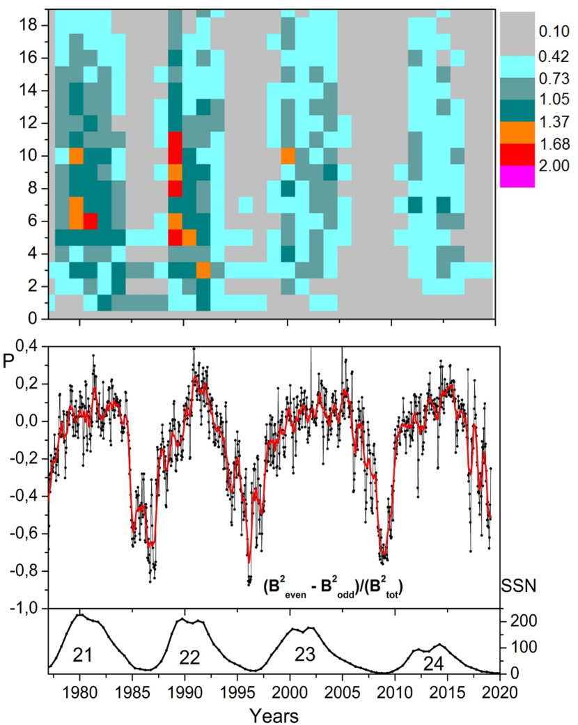
Fig.1 (top panel) represents the contribution of various $l$-harmonics to the mean surface magnetic field versus time. Some prevalence of the even harmonics is visible. The integral parameter, which characterizes the equatorial symmetry of the large-scale magnetic field, is given by the parity index,

$$P=(B_{{\rm even}}^{2}-B_{{\rm odd}}^{2})/(B_{{\rm even}}^{2}+B_{{\rm odd}}^{2}).$$ (6)

It reflects the relative power of the odd and even harmonics in the energy of the large-scale magnetic field. The negative values correspond to the equatorial anti-symmetry ($-1$ - the dipole parity) and the positive values, to the symmetry ($+1$ - the quadrupole parity). This parameter is commonly used in solar dynamo models (Brandenburg et al., 1989; Knobloch et al., 1998; Weiss & Tobias, 2016). From Fig.1 (middle), we see that the solar dynamo shows the dipole-type symmetry during the solar minimum. The solar maximum is characterized by the magnetic field distribution highly asymmetric about the equator. Later, we shall discuss the origin of this phenomenon in more detail.

3.2 Axisymmetric versus non-axisymmetric harmonics

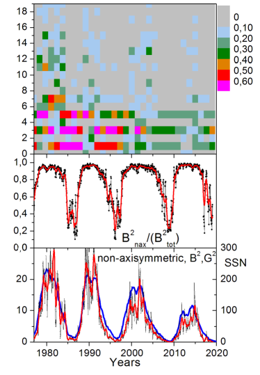
It is interesting that the evolution of the $\ell$ parity of the solar magnetic field seems to be related to the parameters of the axial symmetry. Fig. 2 (top) shows the evolution of the $\ell$ power for the axisymmetric modes of the solar magnetic field during the past four solar cycles. We see its substantial decreases at the end of the observational epoch. This indicates that solar activity has declined substantially in the past two cycles as compared to the end of the XX century. The integral parameter characterizing the relative power of nonaxisymmetric harmonics follows the evolution of the sunspot activity. This parameter is close to unity during the maximum of the sunspot activity (cf, Vidotto et al., 2018). The solar minima show a predominance of the axisymmetric harmonics.

Figure 2: Contribution of each of the first 20 axisymmetric harmonics ($l=0,1,2,...,19$) to the mean magnetic field on the photosphere surface versus time, $m=0$ (top); relative contribution of nonaxisymmetric harmonics ($m\neq 0$) to the mean square magnetic field on the photosphere surface versus time (middle); and total contribution of nonaxisymmetric harmonics to the mean solar magnetic field (bottom). The blue curve on the lower panel shows the solar cycle according to sunspot data.

Figure 3: The smoothed series of the first 4 odd axisymmetric harmonics together with he lowest even axisymmetric harmonic. The data averaged by convolution with the Gaussian function (parameter $\sigma=0.75$).

4 Cyclicity in axisymmetric harmonics

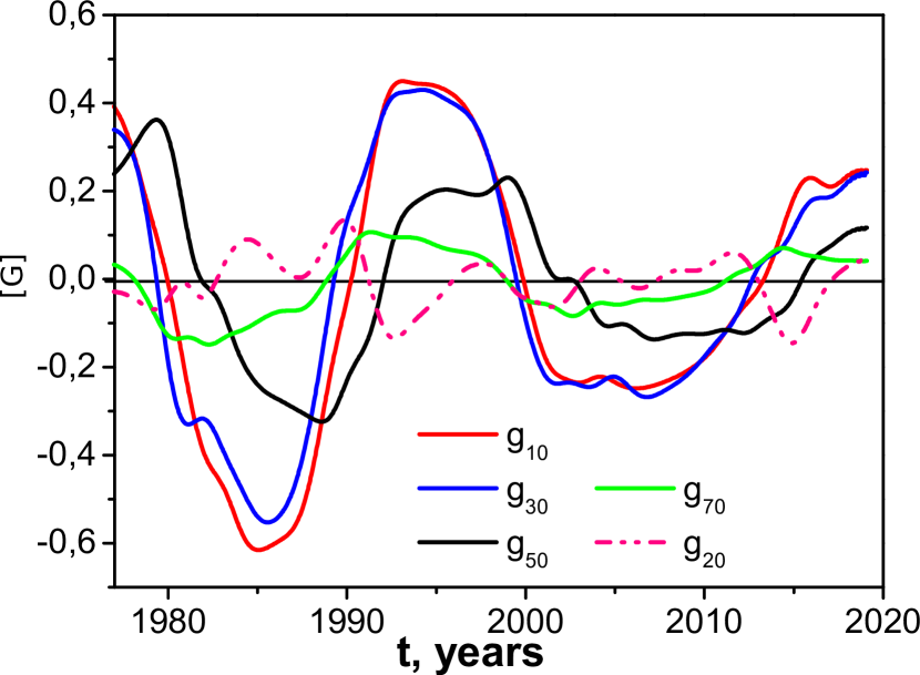
The analysis of the cyclic behavior of axisymmetric modes has run into some difficulties. As seen from Fig. 2, not only the even axisymmetric harmonics, but also the higher-order odd ones yield a chaotic, unrealistic picture. Apparently, taking into account any harmonics of the order higher than $l=7$ results in violation of the regular cyclic dependence (see, Hoeksema, 1995, http://wso.stanford.edu/Polar.html).

Table 1: Phase shifts of the first axisymmetric harmonics with the odd numbers juxtaposed with the phase of the solar cycle as inferred from the polar magnetic field and sunspot data. We have chosen the phase of $g_{50}=0$. The correlation functions (except the one for sunspots) have two maxima and, correspondingly, two estimates of the phase shift. The estimate corresponding to the main maximum of the correlation function is given as the basic value and the other value is added in brackets. The discrepancy between the main quantities and the estimates given in brackets provide us with additional option for measuring the accuracy of the estimates.

	$\Delta t$, years	$\phi$
$g_{10}$	$-2.28$ ($-2.03$)	$0.23\pi$ ($0.20\pi$)
$g_{30}$	$-2.69$ ($-2.29$)	$0.27\pi$ ($0.23\pi$)
$g_{50}$	0	0
$g_{70}$	$-3.69$ ($-3.11$)	$0.37\pi$ ($0.31\pi$)
$B_{{\rm polar}}$	$-1.91$ ($-0.97$)	$0.19\pi$ ($0.10\pi$)
Sunspot number	$3.29$	$-0.33\pi$

Figure 4: a) Integral wavelet spectra for several odd harmonics, the strength of the polar magnetic field and the SN index; b) Correlation coefficients $r$ between $g_{50}$ and the other tracers of solar activity under discussion ($g_{10}$ - red, $g_{30}$ - blue, $g_{50}$ - black, and $g_{70}$ - light green) in comparison with the polar field $B_{{\rm polar}}$ (purple dashed) and sunspots (dark green). The phase of the cycle is given in years (upper horizontal scale) in phase $\phi$ of the whole cycle, which is $2\pi$.

Then, we search for harmonics with a pronounced cyclic behavior and select four such harmonics, namely, $g_{10}$, $g_{30}$, $g_{50}$, and $g_{70}$, Fig. 3. We do not see pronounced cyclicity in axisymmetric harmonics with the even numbers; however, they are interesting as indicators of the North-South asymmetry DeRosa et al., 2012. To be specific, the red dashed line in Fig. 3 show the lowest harmonic $g_{20}$. Despite the activity of $g_{20}$ is irregular it shows a correlation with the polar field reversals (DeRosa et al., 2012). Fig. 3 shows a phase difference in the evolution of the odd axisymmetric harmonics. This difference was analyzed by Stenflo (1994). He found, in particular, that an extended solar cycle in the evolution of the radial magnetic field can inherently result from the evolution of modes, which follows some phase relations. Therefore, the phase relations can shed light on the origin of the solar dynamo. The analysis of Stenflo (1994) was based on the assumption of a unique period for the axisymmetric modes. Here we consider a more general situation.

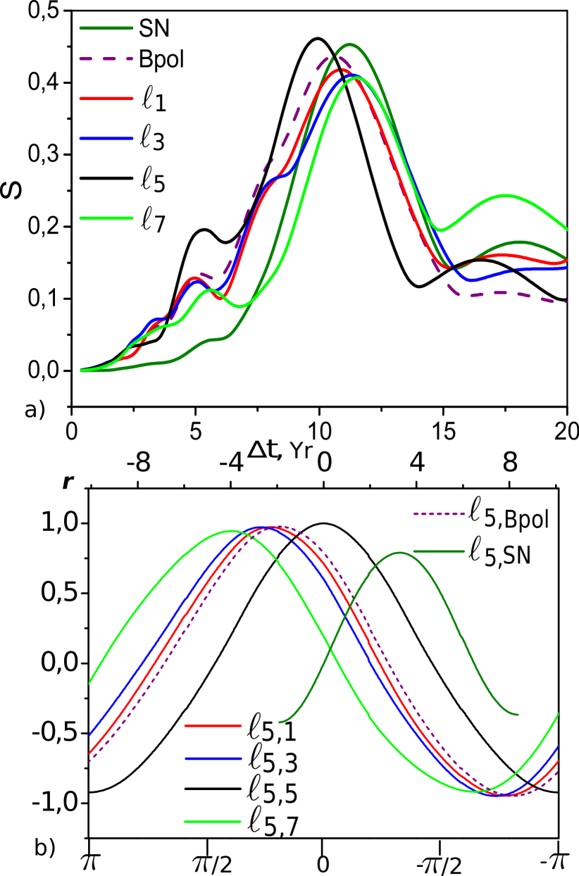
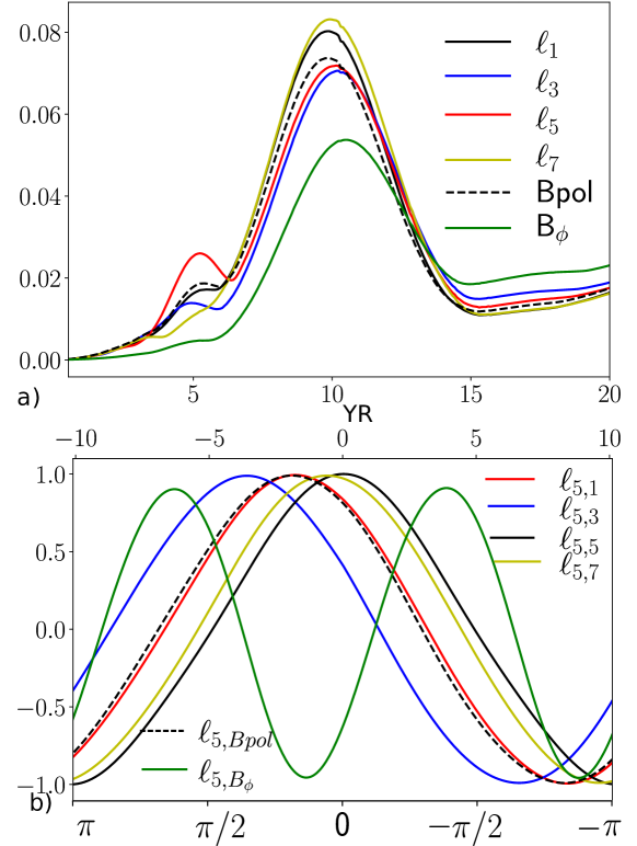
Fig. 4a shows the integral wavelet spectra for the low odd harmonics, the strength of the polar magnetic field and the SN index. The cycle lengths of the modes, as well as the corresponding quantities for the polar filed and the sunspot numbers determined as the location of the maxims in the integral wavelet spectra. They are given in Table 2. One can see, that the different parameters show the different cycle length. Notably, The parameter $g_{50}$ shows the smallest period of about 10 years.

In order to obtain the phase shift between the axisymmetric harmonics and some other tracers of solar activity, we calculate the corresponding correlation coefficients choosing quite arbitrarily the harmonic $g_{50}$ as the basic one. More specifically, we consider two signals, say, $f(t)$ and $g(t)$, shift signal $g$ in time by $\Delta t$, and calculate the correlation function $r$. The result is plotted in Fig. 4b as a function of $\Delta t$. For comparison with Stenflo (1994), we have chosen the phase of $g_{50}$ equal to $0$. Therefore, the mode $g_{50}$ in Fig 4b is shown by the auto-correlation coefficient. In order to compare with the above-cited paper, we have to take into account that the highest correlation is attained by shifting the advance harmonic backward or by shifting the lagged harmonic forward. Therefore, the signs for the time and phase are opposite. Similarly to Stenflo (1994) we find the positive sign for the phase shifts of the all harmonics. Though the magnitude of the shift is about factor twice less than in his study. Recall that $r$ is a dimensionless quantity and $|r|\leq 1$. The location of maximum $r$ for the particular tracer of the solar activity is used as the phase shift of the tracer in respect to the mode $g_{50}$. The autocorrelation coefficient for $g_{50}$ is also shown in the figure for comparison.

Note that the maximum values of $r$ are quite high exceeding 0.9 for $g_{10}$ and $g_{30}$, and even the lowest value (obtained for sunspots) exceeds 0.7. The fact that correlations between the harmonics of the large-scale poloidal magnetic field are larger than their correlations with the polar magnetic field and the correlations with sunspots are even lower looks reasonable because it agrees with the degree of connections between these quantities as expected from the solar dynamo mechanism.

Based on the Fig. 4b, we calculate the corresponding phase shifts as location of the maxima in $\Delta t$ (presented in Table 1). The width of the plot for a particular correlation coefficient allows us to decide how the main phase of the solar cycle is localized for the particular harmonics. In particular, it looks difficult to insist that the phase shifts between $g_{10}$, $g_{30}$, and $B_{{\rm polar}}$ are significant; however, the phase shifts between them and, perhaps, $g_{70}$, $g_{50}$ and sunspots number seem to be significant. It follows from Figure 5b and Table 1 that the sunspot cycle is ahead of the polar field cycle by $\pi/2$, and the $g_{50}$ mode, by $\pi/3$.

Table 2: Cycle lengths of the modes under discussion, polar magnetic field, and sunspot numbers: $T$ is the cycle length for the absolute value, $T_{s}$ is the cycle length for the signed quantities.

	$T$ (years)	$T_{s}$ (years)
$g_{10}$	11.5	23.0
$g_{30}$	11.75	23.5
$g_{50}$	9.75	19.5
$g_{70}$	11.625	23.25
$B_{{\rm polar}}$	10.5	21.0
Sunspot number	11.0	22.0

The analysis of observations can be summarized as follows. The actual phase and length of a nominal 11-year cycle as recorded in such tracers are specific for each harmonic. This was already demonstrated in Stenflo & Vogel (1986), Stenflo (1994) and Knaack & Stenflo (2005). Compared to their work, our analysis covers the period of two full magnetic cycles. Therefore, our conclusions concerning the phases and frequencies of the large-scale magnetic field spherical harmonics are more robust. The low $\ell$ axisymmetric harmonics show a phase shift relative to each other and relative to the proxy of the polar magnetic field strength and the sunspot number index. We have to note that the phase shifts mostly exceed the difference between the mode oscillation periods at least by factor of two. This observation may tell us about the spatial distribution of turbulent sources in the solar dynamo. Indeed, the results of DeRosa et al. (2012) regarding the phase relations between the low $\ell$ harmonics in the Babcock-Leighton type dynamo model show a nearly synchronous evolution of $\ell=1,3$ and $\ell=5$ (see Fig. 15 in DeRosa et al. (2012)). This doesn’t seem surprising, because in their model, the sources of generation of the radial magnetic field are in one place, near the solar surface. Below, we consider the results of the distributed dynamo model that include the effects of emergence of a bipolar region in order to mimic the effects of the sunspot activity on the evolution of the radial magnetic field.

5 Results from mean-field dynamo models

Figure 5: a) The time-latitude diagrams of the toroidal magnetic field (contours in the range of $\pm$1kG) in the subsurface shear layer, r=0.9R and the radial magnetic field on the surface (background image); b) the time-radius diagram for the large-scale magnetic field at the latitude of 30^∘; c) the time-radius evolution of the axisymmetric mode of the radial magnetic field $\ell_{1}$; d), e), and f) show the same for $\ell_{3}$, $\ell_{5}$, and $\ell_{7}$.

Figure 6: Snapshots of the surface magnetic field distributions in a dynamo cycle. The radial magnetic field is shown by color and the toroidal magnetic field, by contours in the same range of $\pm 20$G.

Figure 7: a) $F_{S}$ is the total unsigned flux of the radial magnetic field and $F_{S}^{(ax)}$ is the same for the contribution of the axisymmetric magnetic field; b) $P_{nx}$ is the parameter characterizing the nonaxisymmetry of the surface radial magnetic field, $P_{Br}$ is the equatorial parity parameter of the surface radial magnetic field, and $P_{\widetilde{Br}}$ is the same for the nonaxisymmetric radial magnetic field.

In a preliminary study we considered the results of the run C2 from the axisymmetric dynamo model of Pipin & Kosovichev (2020). A detailed description of the model is given in the above-cited paper. Note that the model explains successfully the so-called “extended” solar cycle (Altrock (1997)) and, besides that, it shows a satisfactory agreement with many aspects of solar observations. However, that model does not take into account the effect of the sunspot activity on the evolution of the radial magnetic field. Despite this, it shows a satisfactory agreement of evolution of the low $\ell$ modes with observations. We provide these results in Appendix B. This model will be a reference in our study of the relative contributions of the deep and surface dynamo processes to the whole magnetic variability of the Sun. To study the possible effects of the sunspot activity on the dynamo evolution, we consider the nonaxisymmetric dynamo model.

We assume that the toroidal magnetic field in the subsurface layer of the convection zone is responsible for the formation of solar bipolar regions in the photosphere. The effect of inclination of the bipolar regions can be parametrized by means of an additional $\alpha$-effect acting on the emerging part of the toroidal magnetic field. This idea follows the phenomenological approach of the Babcock-Leighton dynamo scenario. The mean-field formulation of this scenario was suggested by Nandy & Choudhuri (2001). Here, we follow the same ideas (in particular, see Kumar et al. (2019)). In this scenario, the individual magnetic flux-tubes that rise from the bottom of the convection zone are subject to the effect of the Coriolis force (cf, Cameron & Schüssler, 2017). In the dynamo equations, the averaged effect of this process is described by means of the $\alpha$-effect acting on the axisymmetric magnetic field. Unlike the other parts of the mean electromotive force, the analytical expression of this effect was never obtained from the first principles. In our model we do not apply this ansatz and consider the $\alpha$-effect acting on the buoyant nonaxisymmetric parts of the large-scale toroidal magnetic field. The description of this $\alpha$-effect in our model remains speculative and has a phenomenological character. We simulate the emergence process by means of the magnetic buoyancy of the randomly chosen parts of the axisymmetric toroidal magnetic field in the upper part of the convection zone.

The general consideration shows that the large-scale toroidal magnetic field can be unstable if its strength decreases outward faster than the mean density stratification does (Gilman, 1970). The instability is subjected to effects of the global rotation and turbulent diffusion (Gilman, 1970; Acheson & Gibbons, 1978; Davies & Hughes, 2011; Gilman, 2018). In our model, these effects are not taken into account. The nonaxisymmetric magnetic buoyancy and the related $\alpha$-effect are used in a phenomenological way to generate a solar-like large-scale nonaxisymmetric magnetic field at the dynamo surface. The current knowledge shows that the magnetic buoyancy is unlikely to be the only process responsible for the sunspot formation. All complicated phenomena, such as the effects of convective flows, instabilities due to interaction of the magnetic field and turbulent plasma, and magnetic buoyancy instability, should be taken into account (Kitiashvili et al., 2010; Stein & Nordlund, 2012; Losada et al., 2017). In our model we keep the consideration as simple as possible. Also, we do not try to resolve the real spatial scale of the sunspots active regions. This is rather expensive computationally. The 2D analog of the model was recently discussed by Pipin (2021). The model should be considered as a numerical experiment. It does not pretend to explain the emergence of the solar active regions. The further details concerning the nonaxisymmetric dynamo model are given in the Appendix A.

Figure 5 shows the time-latitude and the time-radius diagrams of the large-scale magnetic field evolution, as well the time-radius evolution of the first four odd axisymmetric spherical harmonics in the nonaxisymmetric dynamo model. The results for the axisymmetric modes $\ell_{1-7}$ are qualitatively similar to the results of the axisymmetric model. However, the time-radius evolution of the radial magnetic field at the latitude of 30^∘ shows the difference. The radial magnetic field generated in the subsurface shear layer drifts downward from the surface and has the opposite sign to the magnetic field propagating from the depth of the convection zone. The poleward surges in the time-latitude diagram of the large-scale radial magnetic field are due to the formation of bipolar regions. There are similar radial surges in the time-radius diagrams.

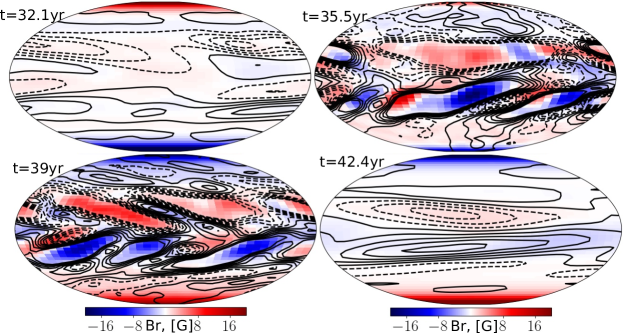
Figure 6 illustrates the snapshots of the surface magnetic field distributions during a dynamo cycle starting from the minimum of the magnetic activity. The model shows solar-like patterns of the magnetic field distribution during the growing and maximum phases of the magnetic activity. Comparing these results with Vidotto et al. (2018), we find that the magnetic field distribution patterns agree with the low-resolution patterns of the magnetic activity found in observations.

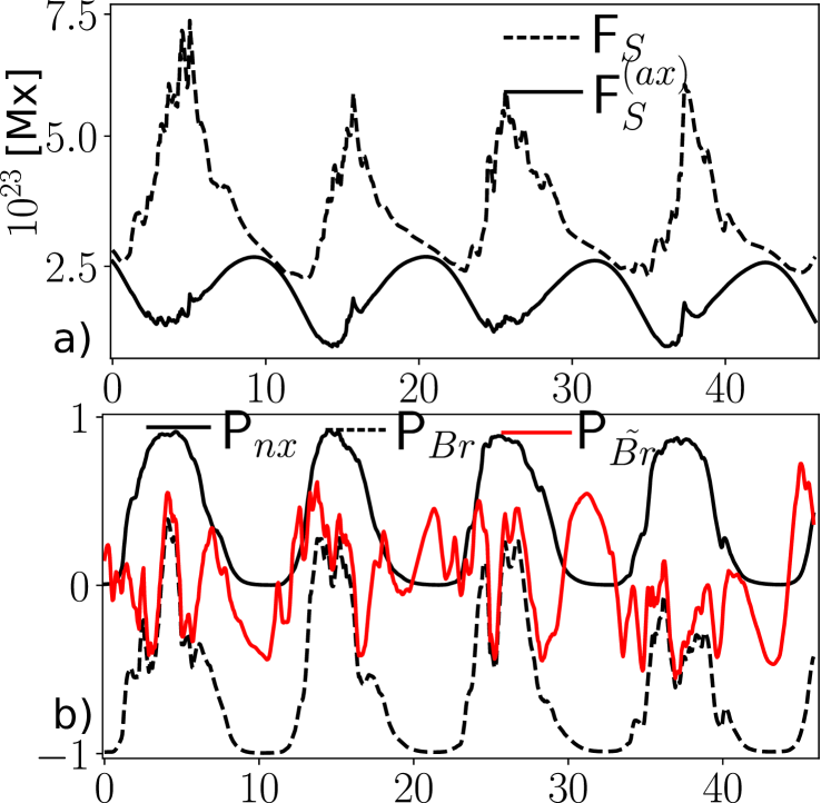
The magnitude of the nonaxisymmetric magnetic field in these snapshots is rather small compared to the sunspot magnetic field. This is due to our model restrictions on the strength and size of the bipolar region. However, the amplitude of the generated radial magnetic field flux agrees with observations to the order of magnitude. The total flux of the radial magnetic field in the model is about 6 10²³ Mx (see Figure7a). This is lower than the value reported by Schrijver & Harvey (1994) (10²⁴Mx) and higher than the flux obtained in the WSO low-resolution observations. The total magnetic flux of the radial magnetic field in the model evolves in phase with the toroidal magnetic field activity in the subsurface shear layer. The magnetic flux of the axisymmetric magnetic field is shifted by $\pi/2$ relative to the evolution of the axisymmetric toroidal magnetic field. Using decomposition of the radial magnetic field into the partial dynamo modes:

$$\left\langle\mathbf{B}_{r}\right\rangle=\sum B_{r}^{(m)}\left(\mu\right)\mathrm{e^{im\phi}},$$

where the case $m=0$ corresponds to the axisymmetric magnetic field, we compute the degree of nonaxisymmetry of the magnetic field:

$$P_{nx} = {\displaystyle\frac{\tilde{E}_{r}^{(m)}}{E_{r}^{(m)}},}$$ (7)

where

$$\tilde{E}_{r}^{(m)}=\frac{1}{8\pi}\sum_{m\geq 1}\intop B_{r}^{(m)}B_{r}^{(m)*}d\mu,$$ (8)

and $E_{r}^{(m)}$ is the total energy of the radial component of the magnetic field. Using decomposition of the radial magnetic field into spherical harmonics, we compute the two parity indices:

$$P_{Br}=\frac{\sum B_{r}^{(\ell_{{\rm even}})2}-\sum B_{r}^{(\ell_{{\rm odd}})2}}{\sum B_{r}^{(\ell)2}},$$ (9)

where summation is done for all modes, and a similar one for the nonaxisymmetric modes:

$$P_{\widetilde{Br}}=\frac{\sum^{m>0}B_{r}^{(\ell_{{\rm even}})2}-\sum^{m>0}B_{r}^{(\ell_{{\rm odd}})2}}{\sum^{m>0}B_{r}^{(\ell)2}}.$$ (10)

Figure 7b shows the evolution of these parameters in the nonaxisymmetric dynamo model. In general we see a qualitative agreement of our results with the observation data represented in Figure 2. In this phase of the magnetic cycle, the parameter $P_{nx}$ is minimum, i.e., the energy of the nonaxisymmetric magnetic field reaches the lowest value.

The model shows substantial variations in the parity parameters of the axisymmetric, $P_{Br}$, and non-axisymmetric, $P_{\widetilde{Br}}$, radial magnetic field. In the model, the emergence of the bipolar region is random in longitude and hemisphere. This induces the hemispheric asymmetry of the sources of the radial magnetic field. In our model the parity varies from -1 to the values which are slightly above zero level. The zero parity means a strong hemispheric asymmetry of the magnetic activity. The obtained parity variations agree with the results of observations shown in Fig.1. The results of our model are qualitatively similar to those demonstrated by the 3D Babcock-Leighton type model of Hazra & Nandy (2019). When comparing the results of the two dynamo models, we have to take into account the difference in the parity parameter definitions. Our definition of the parity parameter reflects the difference between the energy of a symmetric and antisymmetric magnetic field about the equator (see, Brandenburg et al., 1989; Knobloch et al., 1998). Also, our model covers the period of only a few magnetic cycles. The dynamo simulations of (Moss et al., 2008; Weiss & Tobias, 2016; Kitchatinov et al., 2018; Hazra & Nandy, 2019) display much stronger long-term parity variations. The above cited papers show that these variations can result both from fluctuations of the $\alpha$ effect and from hemispheric randomness in the formation of a bipolar region. Such long-term variations are beyond the scope of this paper.

Figure 8: The same as Figures 4 for the nonaxisymmetric dynamo model.

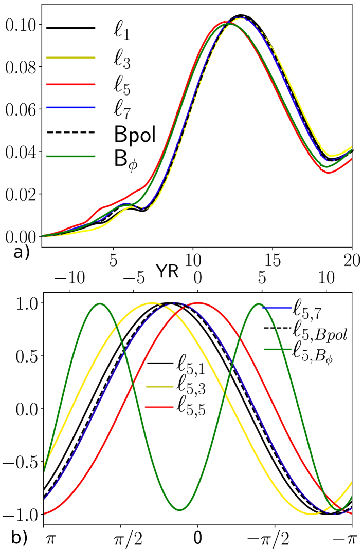
Figure 8 shows the integral wavelets of the low axisymmetric modes and their cross-correlations with the $\ell_{5}$ mode for the nonaxisymmetric dynamo model. The obtained results agree with observations illustrated in Figures 4, except for the phase shift between the modes $\ell_{5}$ and $\ell_{7}$. We find that the effect of nonaxisymmetric magnetic fields brings the correlation between $\ell_{5}$ and the strength of the toroidal magnetic field in agreement with observations.

Table 3: Phase shifts (years) for the run C2 (see, Pipin&Kosovichev, 2020) and the nonaxisymmetric dynamo model (NXDY).

	C2	Period	NXDY,  Period
$g_{10}$	-2.	11.3	-2.5	10.8
	0.17$\pi$		0.23$\pi$
$g_{30}$	-3.45	10.7	-3.9	11.3
	0.3$\pi$		0.37$\pi$
$g_{50}$		11.3	0	10.6
$g_{70}$	1.1	11.3	1.81	10.7
	0.08$\pi$		0.18$\pi$
$B_{{\rm pol}}$	-1.8	11.3	-2.1	10.8
	0.15$\pi$		0.21$\pi$
$B_{\phi}$	3.95	10.6	3.1	10.8
	-0.35$\pi$		-0.29$\pi$

The Table 3 provides the phase shifts and the dynamo periods of the low axisymmetric modes and the integral parameters for our dynamo models.

6 Conclusion and Discussion

Let us summarize the main results of our study. Observations show the difference in the oscillation frequencies of the large-scale magnetic field spherical harmonics. Also, the low $\ell$ axisymmetric harmonics display a phase shift relative to each other and relative to the proxy of the polar magnetic field strength and the sunspot number index. Earlier this phase shift was discussed by Stenflo (1994). Our findings show a a factor twice less shift’s magnitudes. This is likely due to the difference of the time-series interval and the method of analysis. Indeed, the time-series in Fig3 seems to show a twice larger shifts which is in agreement with results of Stenflo (1994) for period before 1990 year. Therefore the times shifts between the $\ell$ harmonics are not constant.

Combining results of this and previous study of DeRosa et al. (2012) we see that the phase shift between the modes depends on the spatial sources of the dynamo processes. For example, the dynamo model by DeRosa et al. (2012) shows nearly synchronous oscillations with the zero phase shift. Our models are based on the distributed dynamo, and they show different phases for the low $\ell$ modes. Both observations and the dynamo model show an exceptional role of the axisymmetric $\ell_{5}$ mode. Its origin seems to be readily connected with the formation and evolution of sunspots on the solar surface. The fluctuating nature of this process can result in a dispersion of the dynamo periods. We find that the cycle periods and the phase shifts of the low $\ell$ modes are different in the axisymmetric and nonaxisymmetric models. Thus, the asynchronous and shifted cycles of the mode can be accounted for both by the specific spatial distribution of the dynamo sources and by nonlinearities involved in the dynamo processes.

In our model, the surface poloidal magnetic field originates from two sources: the poloidal magnetic field, which propagates with the dynamo wave from the depth of the convection zone, and the solar active regions that, in turn, are associated with the dynamo driven toroidal magnetic field in the subsurface shear layer. This is similar to studies of Passos et al. (2014), Hazra et al. (2014) and Hazra & Nandy (2019). Their models employed the Babcock-Leighton type scenario as the main dynamo process. The need for a weak background distributed dynamo was justified by the temporal parameters of the magnetic activity during the Maunder minimum. The relative contribution of both sources is not known in advance and may be specific for each harmonic. The polar magnetic field seems to be most directly connected with the propagation of the poloidal magnetic field from the domain of the solar dynamo action, just because sunspots and active regions are located at middle solar latitudes.

Another interesting observational phenomenon is the excitation of even modes during the maximum phases of the sunspot activity. This results in variation of the parity index $P_{Br}$ around zero (see, Figs.1 and 4). This effect is readily connected with the hemispheric asymmetry of the magnetic activity. It was extensively discussed by DeRosa et al. (2012) and Hazra & Nandy (2019) as the source of long-term variations of the magnetic activity. The models of the Babcock-Leighton type show that the stochastic emergence of active regions and the induced stochastic variations of the $\alpha$-effect can explain both the long-term variations of the solar activity and variations in the hemispheric asymmetry of the activity (Kitchatinov et al., 2018; Bhowmik & Nandy, 2018; Nepomnyashchikh et al., 2019; Hazra & Nandy, 2019). Note, that beating between the modes, when they have close but different periods, is often considered as a source of long-term variation of the solar magnetic activity (Brandenburg et al., 1989; Sokoloff & Nesme-Ribes, 1994; Knobloch et al., 1998; Feynman & Ruzmaikin, 2014; Weiss & Tobias, 2016; Beer et al., 2018). The random fluctuations of the dynamo governing parameters are usually considered as the main drivers of long-term variations of the sunspot activity (see the above cited papers). The long-term parity variations cause a phase-shift between the magnetic activity in the North and South solar hemispheres (e.g., Shibalova et al., 2016; Beer et al., 2018; Hazra & Nandy, 2019). These long-term variations are accompanied by variations in the magnitude and period of a sunspot cycle (Hathaway, 2015). It is likely, that stochastic fluctuations of the dynamo parameters can drive the phase shifts and frequencies of the individual $\ell$ harmonics as well.

Acknowledgements

The authors are grateful to the WSO teams for a free access to their data. The work was supported by RFBR grants No. 20-02-00150,19-52-53045. DS was supported by BASIS found number 18-1-1-77-3. VVP thanks the financial support of the Ministry of Science and Higher Education of the Russian Federation (Subsidy No.075-GZ/C3569/278).

Data Availability Statements. The data underlying this article are available at SIDC (2019). The data of the nonaxisymmetric dynamo model are available at zenodo, Pipin,V.V. (2021).

7 Appendix

A. Nonaxisymmetric dynamo model

Evolution of the large-scale magnetic field in perfectly conductive media is described by the mean-field induction equation Krause & Rädler (1980):

$$\partial_{t}\left\langle\mathbf{B}\right\rangle=\mathbf{\nabla}\times\left(\mathbf{\mathbf{\mathbf{\mathcal{E}}}+}\left\langle\mathbf{U}\right\rangle\times\left\langle\mathbf{B}\right\rangle\right)\,,$$ (11)

where $\mathbf{\mathcal{E}}=\left\langle\mathbf{u\times b}\right\rangle$ is the mean electromotive force; $\mathbf{u}$ and $\mathbf{b}$ are the turbulent fluctuating velocity and magnetic field, respectively; and $\left\langle\mathbf{U}\right\rangle$ and $\left\langle\mathbf{B}\right\rangle$ are the mean velocity and magnetic field. It is convenient to represent the vector $\left\langle\mathbf{B}\right\rangle$ in terms of the axisymmetric and non-axisymmetric components as follows:

$$\left\langle\mathbf{B}\right\rangle = \overline{\mathbf{B}}+\tilde{\mathbf{B}}\,,$$ (12)

$$\mathbf{\overline{B}} = \hat{\mathbf{\phi}}B+\nabla\times\left(A\hat{\mathbf{\phi}}\right)\,,$$ (13)

$$\tilde{\mathbf{B}} = \mathbf{\nabla}\times\left(\mathbf{r}T\right)+\mathbf{\nabla}\times\mathbf{\nabla}\times\left(\mathbf{r}S\right),$$ (14)

where $\overline{\mathbf{B}}$ and $\tilde{\mathbf{B}}$ are the axisymmetric and nonaxisymmetric components, ${A}$, ${B}$, ${T}$ and ${S}$ are the scalar functions representing the field components, $\hat{\mathbf{\phi}}$ is the azimuthal unit vector, $\mathbf{r}$ is the radius vector, $r$ is the radial distance, and $\theta$ is the polar angle. Krause & Rädler (1980) showed that the only gauge transformation for potentials T and S is a sum with the arbitrary r-dependent function. To fix this arbitrariness they suggested the following normalization:

$$\int_{0}^{2\pi}\int_{-1}^{1}Sd\mu d\phi=\int_{0}^{2\pi}\int_{-1}^{1}Td\mu d\phi=0.$$ (15)

We are using the same formulation for the mean electromotive force as in the recent paper by Pipin & Kosovichev (2019):

$$\mathcal{E}_{i} = \mathcal{E}_{i}^{(A)}+\mathcal{E}_{i}^{(P)}\,,$$ (16)

$$\mathcal{E}_{i}^{(A)} = \left(\alpha_{ij}+\gamma_{ij}\right)\left\langle B\right\rangle_{j}-\eta_{ijk}\nabla_{j}\left\langle B\right\rangle_{k},$$

$$\mathcal{E}_{i}^{(P)} = \alpha_{\beta}\delta_{i\phi}\left\langle B\right\rangle_{\phi}-V_{\beta}\left(\hat{\boldsymbol{r}}\times\left\langle\mathbf{B}\right\rangle\right)_{i}\,,$$ (17)

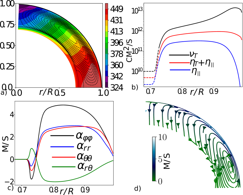
where we divide the expression of the mean electromotive force into the “standard” and phenomenological parts. The standard part of $\mathcal{E}_{i}^{(A)}$ contains contributions of the $\alpha$-effect tensor, $\alpha_{ij}$, the antisymmetric tensor $\gamma_{ij}$ accounts for the turbulent pumping of the large-scale magnetic fields due to the effects of the global rotation and density stratification, and $\eta_{ijk}$ is the eddy magnetic diffusivity tensor. This corresponds to the expression of the mean electromotive force employed in the mean-field dynamo models of Pipin & Kosovichev (2019, 2020). The further details concerning $\mathcal{E}_{i}^{(A)}$ can be found in the above-cited papers. Figure 9 shows the large-scale flow distribution, the radial profiles of the eddy magnetic diffusivity, the $\alpha$-effect, and the effective drift velocity due to the meridional circulation and the turbulent pumping effect.

Figure 9: a) The basic angular velocity profile and the streamlines of the meridional circulation with the maximum circulation velocity of 13 m/s on the surface at the latitude of 45^∘; b) radial profiles of the total, $\eta_{T}+\eta_{||}$, and the rotationally induced part, $\eta_{||}$, of the eddy magnetic diffusivity and the eddy viscosity profile; c) radial profiles of the $\alpha$-effect tensor at the latitude of 45^∘; and d) the effective drift velocity due to the meridional circulation and the turbulent pumping effect.

The phenomenological part of the mean-electromotive force is introduced to account for the surface effects of the emerging magnetic active region on the large-scale dynamo. It is assumed that the toroidal magnetic field in the upper part of the convection zone can be buoyantly unstable and forms magnetic bipolar regions on the solar surface. Following Pipin & Kosovichev (2018) we put

$$V_{\beta} = -\frac{\alpha_{MLT}u^{\prime}}{\gamma}\beta^{2}K\left(\beta\right)\left(1+\xi_{\beta}(t,r,\phi,\theta)\right)\,,$$ (18)

where $\mathrm{\alpha_{MLT}}=1.9$ is the mixing-length theory parameter, $\gamma$ is the adiabatic law constant, $\mathbf{\boldsymbol{\Lambda}}^{(\rho)}=\boldsymbol{\nabla}\log\overline{\rho}$; functions $f_{1,3}^{(a)}$ and $K\left(\beta\right)$ are given in Kitchatinov & Pipin (1993). The parameter $\xi_{\beta}$ determines the magnetic buoyancy velocity perturbations. The position of the unstable layer was computed following the consideration of Parker (1979). It is assumed that the large-scale toroidal magnetic field becomes unstable when its strength decreases outward faster than the mean density does. In particular, we compute the parameter

$$I=-r\frac{\partial}{\partial r}\log\left(\frac{\overline{B}}{\overline{\rho}}\right),$$ (19)

where $\overline{B}$ is the strength of the toroidal magnetic field and $\overline{\rho}$ is the density profile. For the unstable part of the toroidal magnetic field $I>0$. Note, that the magnetic buoyancy instability can be affected by the stellar turbulence and the global rotation (Gilman, 1970; Acheson & Gibbons, 1978; Davies & Hughes, 2011; Gilman, 2018). We do not consider these effects in our simple model. Figure 10 shows snapshots of the magnetic field and the instability parameter distributions during the growing phase of the magnetic cycle. We see, that in our model the unstable layers of the toroidal magnetic field are connected with the bottom of the convection zone and the subsurface shear layer.

Figure 10: a) Snapshot of the axisymmetric magnetic field distribution in the convection zone in the growing phase of the magnetic cycle, color shows the toroidal magnetic field strength and contours show streamlines of the poloidal magnetic field (solid lines - clockwise direction); b) color image shows the instability parameter I (see, Eq19), contour line shows the toroidal magnetic field strength of 500G.

Figure 11: The same as Fig.8 for axisymmetric dynamo model.

Figure 12: The same as Fig.5 for axisymmetric dynamo model.

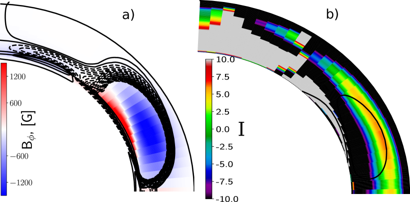
The $\xi_{\beta}$ perturbations are initiated within the upper layer $I>0$; initiations are random in time. They go as a Gaussian sequence with the mean cadence equal to a month. The Gaussian sequences of $\xi_{\beta}$ in the north and south hemispheres are independent. Similar to Pipin & Kosovichev (2018), we define $\xi_{\beta}$ as follows,

$$\!\xi_{\beta}\!=\!C_{\beta}\!\psi\negthinspace\exp\left(\!-m_{\beta}\left(\!\sin^{2}\!\left(\!\frac{\phi-\phi_{0}}{2}\!\right)\!+\!\sin^{2}\!\left(\!\frac{\theta-\theta_{\mathrm{m}}}{2}\!\right)\!\right)\!\right)\!,$$ (20)

where $\psi$ is a kink-type function in radius and time,

$$\psi\!\! =\!\! \frac{1}{2}\left(\!1\!-\!\mathrm{erf}\left(50\left(r-r_{m}\right)\right)^{2}\!\right)\!\mathrm{e}\!^{{\displaystyle-\left(\frac{\tau_{0}-t}{2\tau_{0}}\right)^{2}}}\!,t\!<\!\delta t$$

$$= 0,t>\delta t\,,$$

the longitude $\phi_{0}$ is random; $\theta_{m}$ and $r_{m}$ are the latitude and radius of the extreme points of the toroidal magnetic field in the upper part of the convection zone, where the instability parameter $I>0$. We restrict the active phase time, $\delta t$, of the bipolar region evolution to one week. The emergence interval of the bipolar region is controlled by the parameter $\tau_{0}$. In our simulations we put it to 3 days, which corresponds to the observation results (see, Stenflo & Kosovichev (2012)). The parameter $C_{\beta}=200$ is chosen in such a way that the unstable part of the axisymmetric magnetic field could emerge on the surface after time $\tau_{0}$ starting from the level r=0.9R, which corresponds to the mean level of the magnetic buoyancy instability of the large-scale toroidal magnetic field in the upper part of the convection zone. In this model we do not intend to reproduce the spatial parameters of the sunspot bipolar regions. For the sake of numerical efficiency we put $m_{\beta}=20$, which results in large-scale bipolar regions, (see, Figure 6). The $\alpha$-effect will be given as follows

$$\alpha_{\beta}=0.3\cos\theta V_{\beta},$$ (22)

where $V_{\beta}$ is determined by Eq(18), and the coefficient $0.3$ was chosen from numerical experiments. With our representation of the mean electromotive force in the form of Eq(16), the full version of the dynamo equations for the axisymmetric magnetic field reads as follows,

$$\partial_{t}A = \mathcal{E}_{\phi}^{(A)}+\overline{\alpha_{\beta}\left\langle B_{\phi}\right\rangle}+\frac{V_{\beta}}{r}\frac{\partial\left(rA\right)}{\partial r}+\overline{V_{\beta}\tilde{B}_{\theta}},$$ (23)

$$\partial_{t}B = \frac{\sin\theta}{r}\frac{\partial\left(r\sin\theta A,\Omega\right)}{\partial\left(r,\mu\right)}-\frac{1}{r}\frac{\partial}{\partial r}r^{2}\left(V_{\beta}B+\overline{V_{\beta}\tilde{B}_{\phi}}\right)$$ (24)

$$+ \frac{1}{r}\frac{\partial r\mathcal{E}_{\theta}^{(A)}}{\partial r}+\frac{\sqrt{\left(1-\mu^{2}\right)}}{r}\frac{\partial\mathcal{E}_{r}^{(A)}}{\partial\mu}\,,$$

where, the contribution of $\mathcal{E}^{(A)}$ stands for the standard part of the mean-electromotive force, its details are omitted. For the sake of brevity, the $\alpha_{\beta}$-effect and magnetic buoyancy terms are written explicitly via the magnetic field components. Besides, these contributions bear the effect of the nonlinear coupling between the axisymmetric and nonaxisymmetric modes of the magnetic field. For example, we have $\overline{\alpha\left\langle B\right\rangle_{\phi}}=\overline{\alpha}B+\overline{\tilde{\alpha}\tilde{B}_{\phi}}$ and the same is true for other similar terms. Note that the second part of this formula, the term $\overline{\tilde{\alpha}\tilde{B}_{\phi}}$, as well as the terms like $\overline{\alpha_{\beta}\left\langle B\right\rangle_{\phi}}$ and similar ones that are related to the magnetic buoyancy, are usually ignored in standard mean-field dynamo models. In general, we can see some similarity between the effect due to $\overline{\tilde{\alpha}\tilde{B}_{\phi}}$ and the non-local $\alpha$-effect employed in the flux-transport models (Cameron & Schüssler, 2017). In our approach, we explicitly take into account the dynamics of the nonaxisymmetric magnetic field and its averaged effect on the evolution of the large-scale magnetic field. To get the evolution equation for the nonaxisymmetric potential $S$ we substitute Eq(14) into Eq(11) and, then, calculate the scalar product with vector $\mathbf{\hat{r}}$. Similarly, the equation for $T$ is obtained by taking curl of Eq(11) and, then, the scalar product with vector $\mathbf{\hat{r}}$. The procedure was described in detail by Krause & Rädler (1980). See also Bigazzi & Ruzmaikin (2004) and Pipin & Kosovichev (2015). The equations for the potentials T and S are

$$\partial_{t}\Delta_{\Omega}S = \Delta_{\Omega}U^{(U)}+\Delta_{\Omega}U^{(\mathcal{E}A)}+\Delta_{\Omega}U^{(\mathcal{E}P)},$$ (25)

$$\partial_{t}\Delta_{\Omega}T = \Delta_{\Omega}V^{(U)}+\Delta_{\Omega}V^{(\mathcal{E}A)}+\Delta_{\Omega}V^{(\mathcal{EP})},$$ (26)

where we introduce new notations

$$\Delta_{\Omega}V^{(U)} = -\hat{\mathbf{r}}\cdot\boldsymbol{\nabla}\times\boldsymbol{\nabla}\times\left(\mathbf{\overline{U}}\times\mathbf{\tilde{\mathbf{B}}}\right),$$ (27)

$$\Delta_{\Omega}V^{(\mathcal{E})} = -\hat{\mathbf{r}}\cdot\boldsymbol{\nabla}\times\boldsymbol{\nabla}\times\boldsymbol{\boldsymbol{\mathcal{E}}},$$ (28)

$$\Delta_{\Omega}U^{(U)} = -\hat{\mathbf{r}}\cdot\boldsymbol{\nabla}\times\left(\mathbf{\overline{U}}\times\tilde{\mathbf{B}}\right),$$ (29)

$$\Delta_{\Omega}U^{(\mathcal{E})} = -\hat{\mathbf{r}}\cdot\boldsymbol{\nabla}\times\boldsymbol{\boldsymbol{\mathcal{E}}}.$$ (30)

We do not show details of $\Delta_{\Omega}U,V^{(U)}$ as well as the standard parts of the $\Delta_{\Omega}U,V^{(\mathcal{E})}$ terms. Their derivation is described in detail in the above-cited papers. For the nonaxisymmetric parts related to the magnetic buoyancy and $\alpha_{\beta}$ the effect reads as follows

$$\Delta_{\Omega}V^{(\mathcal{E}P)} = -\frac{1}{r\sin\theta}\frac{\partial}{\partial\phi}\frac{\partial}{\partial r}\left(r\left\langle B_{\theta}\right\rangle V_{\beta}\right)$$

$$- \frac{\partial}{\partial\mu}\left(\frac{\sin\theta}{r}\frac{\partial}{\partial r}\left(r\left\langle B_{\phi}\right\rangle V_{\beta}\right)\right)$$

$$- \frac{1}{r}\frac{\partial}{\partial r}r\left[\frac{1}{\sin\theta}\frac{\partial}{\partial\phi}\alpha_{\beta}\left\langle B_{\phi}\right\rangle\right],$$

$$\Delta_{\Omega}U^{(\mathcal{E}P)} = -\frac{1}{\sin\theta}\frac{\partial}{\partial\phi}\left(\left\langle B_{\phi}\right\rangle V_{\beta}\right)+\frac{\partial}{\partial\mu}\left(\sin\theta\left\langle B_{\theta}\right\rangle V_{\beta}\right)$$

$$+ \frac{\partial}{\partial\mu}\alpha_{\beta}\left\langle B_{\phi}\right\rangle.$$

B. Results of axisymmetric dynamo model

Here we reproduce some results of the run C2 from Pipin & Kosovichev (2020). See the above-cited paper for details of the model. Figure 11a shows variations in the first four odd axisymmetric spherical harmonics on the surface, as well as the evolution of the mean polar magnetic field and the mean density of the toroidal field in the subsurface layer, $r=0.9-0.99R$. The parameter $\overline{B_{\phi}}$ is considered a proxy for the sunspot number. The integral wavelets of the low axisymmetric modes and their cross-correlations with $\ell_{5}$ mode are shown in Figure11b. The toroidal magnetic field and the $\ell_{3}$ harmonic show periods of about 10.6 years. The polar magnetic field, as well as the $\ell_{1,5,7}$ axisymmetric harmonics show a period of about 11.3 years. The axisymmetric modes show an auxiliary peak around 5 years. In the axisymmetric model, the correlation of the mode $\ell_{5}$ with other axisymmetric modes, as well as with the integral parameters $B_{pol}$ and the sunspot proxy $B_{\phi}$ agrees qualitatively with observations (see, Figure11b). The correlation between $\ell_{5}$ and $\ell_{7}$ shows the largest difference compared to the observation results. The time-latitude and time-radius diagrams of the large-scale magnetic field evolution, as well as the time-radius evolution of the first four odd axisymmetric spherical harmonics are shown in Figure 12. The butterfly diagram of the model qualitatively agrees with observations. At the latitude of 30^∘, the diagram of the time-radius evolution of the toroidal and radial magnetic field shows a drift of the magnetic field activity toward the surface. The duration of the drift is about half a magnetic cycle. It is interesting to note that the axisymmetric harmonics $\ell_{1}$ and $\ell_{7}$ follow the same direction of the drift. The $\ell_{3}$ harmonic shows a steady wave with two maxima: one near the bottom and the other at the top of the convection zone. The $\ell_{5}$ harmonic shows a similar tendency. However its maximum at the top of the convection zone is less pronounced than for the $\ell_{3}$ . In the upper part of the convection zone, $\ell_{5}$ displays an inward drift. Therefore, the model evolution of the radial magnetic field of $\ell_{3}$ and $\ell_{5}$ harmonics can be connected with the toroidal magnetic field in the subsurface shear layer. Naturally, the $\ell_{5}$ maxima at the surface correspond to the maxima of the toroidal magnetic field butterfly diagrams.

The above consideration reveals the peculiarities in the evolution of the $\ell_{3}$ and $\ell_{5}$ axisymmetric harmonics of the radial magnetic field. The harmonic $\ell_{3}$ displays a dynamo period close to the period of the toroidal magnetic field parameter $\overline{B_{\phi}}$ in the subsurface layer. This harmonic is shifted ahead by about $\pi/2$ of the toroidal magnetic field evolution and has its maximum at the surface. Therefore, the surface evolution of $\ell_{3}$ is determined by generation of the radial magnetic field from the toroidal magnetic field by means of the $\alpha$-effect. While the generation of $\ell_{3}$ is connected with the rising branch of the toroidal magnetic field in the subsurface shear layer, the near-surface generation of $\ell_{5}$ is connected with the decaying $\overline{B_{\phi}}$ there. Observations show that the periods of $\ell_{5}$ and $\overline{B_{\phi}}$ are close. This means that there may be an additional near-surface source of the $\alpha$-effect that produces $\ell_{5}$. We assume that it can be due to the emerging bipolar regions.

References

- Acheson & Gibbons (1978) Acheson D. J., Gibbons M. P., 1978, Journal of Fluid Mechanics, 85, 743
- Altrock (1997) Altrock R. C., 1997, Sol. Phys., 170, 411
- Beer et al. (2018) Beer J., Tobias S. M., Weiss N. O., 2018, MNRAS, 473, 1596
- Benevolenskaya (2004) Benevolenskaya E. E., 2004, A&A, 428, L5
- Bhowmik & Nandy (2018) Bhowmik P., Nandy D., 2018, Nature Communications, 9, 5209
- Bigazzi & Ruzmaikin (2004) Bigazzi A., Ruzmaikin A., 2004, ApJ, 604, 944
- Brandenburg (2005) Brandenburg A., 2005, Astrophys. J., 625, 539
- Brandenburg (2018) Brandenburg A., 2018, Journal of Plasma Physics, 84, 735840404
- Brandenburg et al. (1989) Brandenburg A., Krause F., Meinel R., Moss D., Tuominen I., 1989, A&A, 213, 411
- Cameron & Schüssler (2017) Cameron R. H., Schüssler M., 2017, A&A, 599, A52
- Charbonneau (2020) Charbonneau P., 2020, Living Reviews in Solar Physics, 2, 2
- Dasi-Espuig et al. (2010) Dasi-Espuig M., Solanki S. K., Krivova N. A., Cameron R., Peñuela T., 2010, A&A, 518, A7
- Davies & Hughes (2011) Davies C. R., Hughes D. W., 2011, ApJ, 727, 112
- DeRosa et al. (2012) DeRosa M. L., Brun A. S., Hoeksema J. T., 2012, ApJ, 757, 96
- Feynman & Ruzmaikin (2014) Feynman J., Ruzmaikin A., 2014, Journal of Geophysical Research (Space Physics), 119, 6027
- Gilman (1970) Gilman P. A., 1970, ApJ, 162, 1019
- Gilman (2018) Gilman P. A., 2018, ApJ, 867, 45
- Gizon et al. (2020) Gizon L., Cameron R. H., Pourabdian M., Liang Z.-C., Fournier D., Birch A. C., Hanson C. S., 2020, Science, 368, 1469
- Gokhale & Javaraiah (1992) Gokhale M. H., Javaraiah J., 1992, Sol. Phys., 138, 399
- Gokhale et al. (1992) Gokhale M. H., Javaraiah J., Kutty K. N., Varghese B. A., 1992, Sol. Phys., 138, 35
- Hathaway (2015) Hathaway D. H., 2015, Living Reviews in Solar Physics, 12, 4
- Hazra & Nandy (2019) Hazra S., Nandy D., 2019, MNRAS, 489, 4329
- Hazra et al. (2014) Hazra S., Passos D., Nandy D., 2014, ApJ, 789, 5
- Hoeksema (1984) Hoeksema J. T., 1984, PhD thesis, Stanford Univ., CA.
- Hoeksema (1991) Hoeksema J. T., 1991, Advances in Space Research, 11, 15
- Hoeksema (1995) Hoeksema J. T., 1995, Space Sci. Rev., 72, 137
- Howe et al. (2011) Howe R., Larson T. P., Schou J., Hill F., Komm R., Christensen-Dalsgaard J., Thompson M. J., 2011, Journal of Physics Conference Series, 271, 012061
- Käpylä et al. (2016) Käpylä M. J., Käpylä P. J., Olspert N., Brandenburg A., Warnecke J., Karak B. B., Pelt J., 2016, A&A, 589, A56
- Kitchatinov & Pipin (1993) Kitchatinov L. L., Pipin V. V., 1993, A&A, 274, 647
- Kitchatinov et al. (2018) Kitchatinov L. L., Mordvinov A. V., Nepomnyashchikh A. A., 2018, A&A, 615, A38
- Kitiashvili et al. (2010) Kitiashvili I. N., Kosovichev A. G., Wray A. A., Mansour N. N., 2010, ApJ, 719, 307
- Knaack & Stenflo (2005) Knaack R., Stenflo J. O., 2005, A&A, 438, 349
- Knobloch et al. (1998) Knobloch E., Tobias S. M., Weiss N. O., 1998, MNRAS, 297, 1123
- Kosovichev et al. (2013) Kosovichev A. G., Pipin V. V., Zhao J., 2013, in Shibahashi H., Lynas-Gray A. E., eds, Astronomical Society of the Pacific Conference Series Vol. 479, Progress in Physics of the Sun and Stars: A New Era in Helio- and Asteroseismology. p. 395 (arXiv:1402.1901)
- Krause & Rädler (1980) Krause F., Rädler K.-H., 1980, Mean-Field Magnetohydrodynamics and Dynamo Theory. Berlin: Akademie-Verlag
- Kumar et al. (2019) Kumar R., Jouve L., Nandy D., 2019, A&A, 623, A54
- Levine (1977) Levine R. H., 1977, ApJ, 218, 291
- Losada et al. (2017) Losada I. R., Warnecke J., Glogowski K., Roth M., Brandenburg A., Kleeorin N., Rogachevskii I., 2017, in Vargas Domínguez S., Kosovichev A. G., Antolin P., Harra L., eds, IAU Symposium Vol. 327, Fine Structure and Dynamics of the Solar Atmosphere. pp 46–59 (arXiv:1704.04062), doi:10.1017/S1743921317004306
- Moss et al. (2008) Moss D., Sokoloff D., Usoskin I., Tutubalin V., 2008, Solar Phys., 250, 221
- Nandy & Choudhuri (2001) Nandy D., Choudhuri A. R., 2001, ApJ, 551, 576
- Nepomnyashchikh et al. (2019) Nepomnyashchikh A., Mandal S., Banerjee D., Kitchatinov L., 2019, A&A, 625, A37
- Obridko & Yermakov (1989) Obridko V. N., Yermakov F. A., 1989, Astronomicheskij Tsirkulyar, 1539, 24
- Obridko et al. (2020) Obridko V. N., Sokoloff D. D., Shelting B. D., Shibalova A. S., Livshits I. M., 2020, MNRAS, 492, 5582
- Parker (1979) Parker E. N., 1979, Cosmical magnetic fields: Their origin and their activity. Oxford: Clarendon Press
- Passos et al. (2014) Passos D., Nandy D., Hazra S., Lopes I., 2014, A&A, 563, A18
- Pipin (2021) Pipin V. V., 2021, Journal of Plasma Physics, 87, 775870101
- Pipin & Kosovichev (2015) Pipin V. V., Kosovichev A. G., 2015, The Astrophysical Journal, 813, 134
- Pipin & Kosovichev (2018) Pipin V. V., Kosovichev A. G., 2018, ApJ, 867, 145
- Pipin & Kosovichev (2019) Pipin V. V., Kosovichev A. G., 2019, ApJ, 887, 215
- Pipin & Kosovichev (2020) Pipin V. V., Kosovichev A. G., 2020, ApJ, 900, 26
- Pipin,V.V. (2021) Pipin,V.V. 2021, Data of nonaxisymmetric dynamo model, doi:10.5281/zenodo.4662308
- SIDC (2019) SIDC 2019, Monthly Report on the International Sunspot Number, online catalogue, http://www.sidc.be/sunspot-data/
- Scherrer et al. (1977) Scherrer P. H., Wilcox J. M., Svalgaard L., Duvall T. L. J., Dittmer P. H., Gustafson E. K., 1977, Sol. Phys., 54, 353
- Schrijver & Harvey (1994) Schrijver C. J., Harvey K. L., 1994, Sol. Phys., 150, 1
- Shibalova et al. (2016) Shibalova A. S., Obridko V. N., Sokoloff D. D., 2016, Astronomy Reports, 60, 949
- Sokoloff & Nesme-Ribes (1994) Sokoloff D., Nesme-Ribes E., 1994, A&A, 288, 293
- Stein & Nordlund (2012) Stein R. F., Nordlund Å., 2012, ApJ, 753, L13
- Stejko et al. (2021) Stejko A. M., Kosovichev A. G., Pipin V. V., 2021, arXiv e-prints, p. arXiv:2101.01220
- Stenflo (1994) Stenflo J. O., 1994, in Rutten R. J., Schrijver C. J., eds, NATO Advanced Study Institute (ASI) Series C Vol. 433, Solar Surface Magnetism. p. 365
- Stenflo & Kosovichev (2012) Stenflo J. O., Kosovichev A. G., 2012, ApJ, 745, 129
- Stenflo & Vogel (1986) Stenflo J. O., Vogel M., 1986, Nature, 319, 285
- Stenflo & Weisenhorn (1987) Stenflo J. O., Weisenhorn A. L., 1987, Sol. Phys., 108, 205
- Svalgaard et al. (1978) Svalgaard L., Duvall T. L. J., Scherrer P. H., 1978, Sol. Phys., 58, 225
- Usoskin (2017) Usoskin I. G., 2017, Living Reviews in Solar Physics, 14, 3
- Vidotto et al. (2018) Vidotto A. A., Lehmann L. T., Jardine M., Pevtsov A. A., 2018, MNRAS, 480, 477
- Wang et al. (1989) Wang Y. M., Nash A. G., Sheeley N. R. J., 1989, ApJ, 347, 529
- Warnecke et al. (2018) Warnecke J., Rheinhardt M., Tuomisto S., Käpylä P. J., Käpylä M. J., Brandenburg A., 2018, A&A, 609, A51
- Weiss & Tobias (2016) Weiss N. O., Tobias S. M., 2016, MNRAS, 456, 2654