Influence of individual nodes
for continuous-time Susceptible-Infected-Susceptible dynamics
on synthetic and real-world networks

Abstract

In the study of epidemic dynamics a fundamental question is whether a pathogen initially affecting only one individual will give rise to a limited outbreak or to a widespread pandemic. The answer to this question crucially depends not only on the parameters describing the infection and recovery processes but also on where, in the network of interactions, the infection starts from. We study the dependence on the location of the initial seed for the Susceptible-Infected-Susceptible epidemic dynamics in continuous time on networks. We first derive analytical predictions for the dependence on the initial node of three indicators of spreading influence (probability to originate an infinite outbreak, average duration and size of finite outbreaks) and compare them with numerical simulations on random uncorrelated networks, finding a very good agreement. We then show that the same theoretical approach works fairly well also on a set of real-world topologies of diverse nature. We conclude by briefly investigating which topological network features determine deviations from the theoretical predictions.

I Introduction

As the present pandemic keeps reminding us, disease spreading plays in our world a role that can hardly be overestimated [1]. To understand how an infectious pathogen in a single individual develops into a widespread epidemic it is crucial to investigate the relationship between the topology of the interaction pattern and the collective properties of the contagion [2, 3]. Among the nontrivial questions that spreading phenomena in complex networks raise, the effect of the exact location where the contagion is seeded is one of the most interesting. Is the course of an epidemic strongly depending on where the pathogen first appears? Is it possible to calculate this dependence, thus identifying a priori influential spreaders to be monitored? Are purely topological quantities (centralities) able to provide information on the size or duration of an outbreak started in a given node? After the seminal paper by Kitsak et al. [4] these questions have attracted a lot of interest. The natural framework for investigating these issues is the stochastic Susceptible-Infected-Removed (SIR) model, where susceptible nodes can be infected by neighboring nodes in a network and then spontaneously recover, acquiring permanent immunity. Spreading influence is naturally measured by considering the average final size $S_{n}$ of an outbreak originated by a seed placed in node $n$. Such a quantity is finite (on any finite network) for any value of the parameters describing the dynamics. Initially, the focus has been on the identification of topological centralities, such as degree, K-core or eigenvalue centrality, sufficiently correlated with outbreak size, in the sense that ranking nodes based on the centrality provides the correct ranking also for what concerns $S_{n}$. Many methods and associated quantities have been considered to perform this goal [5]. The mapping of SIR static properties to bond percolation has allowed to recognize Non-Backtracking centrality as the solution of the problem for random networks at criticality [6] and to calculate, via message-passing methods, the spreading influence throughout the whole phase-diagram [7].

Concerning instead epidemic processes without permanent immunity (such as the Susceptible-Infected-Susceptible, SIS) activity has been much more limited [8, 9], because in this case the very definition of spreading influence is not trivial, since above the epidemic threshold a fraction of all outbreaks lasts indefinitely in time. Very recently, we have tackled this issue and studied the problem of influential spreaders for SIS dynamics in discrete time [10]. In that paper, we have considered three different quantities that measure spreading influence and applied an existing theoretical framework [11] (conceptually equivalent to the quenched mean-field approach [2]) to calculate them analytically. Numerical simulations, performed on random uncorrelated networks, have confirmed the validity of the approach, revealing a satisfactory overall agreement with the theoretical predictions.

While the work in Ref. [10] constitutes a first systematic approach to the study of spreading influence for SIS dynamics in networks, some questions remain open. The first has to do with the extension of the results to SIS in continuous time, which is, in many respects, a more realistic model for infectious disease. The framework of Ref. [11] is easily applicable to a discrete time dynamics where, in particular, the duration of the infected state is set deterministically to 1 for all individuals. Because of that, at the same time a node gets infected, the node that transmitted the infection to it (infector) necessarily becomes susceptible again. This is very different from what happens when the duration of the infected state is a random variate (as in continuous-time SIS): in such a case the infector remains infected for some time after the infection event, so that the effective degree of the newly infected individual for further spreading the disease is temporarily reduce by one. These dynamical correlations among the state of neighbors make the application of the approach of Larremore et al. to SIS in continuous time nontrivial and in principle less accurate.

Another relevant question left completely open is the validity of the approach beyond random uncorrelated networks. Real-world topologies are in general very different from the synthetic networks considered in Ref. [10], as they may include arbitrary degree distributions and correlations, local clustering, mesoscopic structures (communities, core-periphery) and so on. Is the theoretical approach able to accurately describe spreading influence also for such interaction patterns? How do different topological properties affect the predictive power of the theory?

In this paper we tackle these major questions, providing an exhaustive response to the first and, by investigating the SIS model on a set of real-world structures, highlighting the different role that some topological properties play in determining the validity of the approach on generic networks.

II Theoretical approach

We consider the standard SIS dynamics in continuous time on an undirected unweighted network. Each node $i$ can be either susceptible or infected. Infection and healing dynamics are ruled by two Poisson processes. At rate (probability per unit time) $\mu$ each infected node recovers spontaneously, becoming susceptible again. An infected node may transmit the contagion to each of its susceptible neighbors. This occurs independently at rate $\beta$ for each one of the susceptible neighbors. We consider an initial condition with a single node $n$ infected, while all the others are in the susceptible state and we are interested in calculating the dependence on the seed node $n$ of the probability $b_{n}$ to observe a finite outbreak, of the average duration $T_{n}$ and of the average size $S_{n}$ of finite outbreaks [10].

II.1 Quenched Mean-Field theory

Inspired by the approach developed by Larremore et al. in Ref. [11], we write an equation for the probability $c_{n}(t)$ that an outbreak starting from a seed node $n$ has a duration smaller than or equal to $t$. We compute it by means of a one-step calculation, considering the system with only node $n$ infected at time $t=0$ and making the assumption of a locally tree-like network, so that we can consider outbreaks propagating to the different neighbors of $n$ as independent. To do so, we consider the probability $c_{n}(t+dt)$ that a seed node $n$ generates an outbreak of duration smaller than or equal to $t+dt$, with $dt$ an infinitesimal time interval. Due to the Poisson nature of the infection and healing processes, in the interval $dt$ the node $n$ can heal with probability $\mu dt$ and can infect each of its $k_{n}$ nearest neighbors with probability $\beta dt$. Otherwise, with probability $1-\mu dt-k_{n}\beta dt$, nothing happens. If a recovery event takes place, then the outbreak stops and consequently its duration is necessarily smaller than any $t^{\prime}>dt$. If the node infects one of its nearest neighbors, the newly infected node $m$, together with the seed node $n$, still infected, can give rise to another outbreak, starting at time $t=dt$ from the pair $(n,m)$ of infected neighbors. For the global outbreak to be shorter than $t+dt$, this induced outbreak must have a duration shorter than $t$. If nothing happens, the node $n$ will still be infected at time $dt$, so we must impose that the subsequent outbreak it generates has a duration not larger than $t$. Denoting by $c_{nm}(t)$ the probability that the adjacent pair of infected nodes $(n,m)$ generate an outbreak of duration not larger than $t$, we can write

$$c_{n}(t+dt) = \mu dt+\bigl{[}1-(\mu+k_{n}\beta)dt\bigr{]}c_{n}(t)$$ (1)

$$+ \sum\limits_{m}a_{nm}\beta dtc_{mn}(t),$$

where $a_{nm}$ is the adjacency matrix of the network, and we assume that the duration probabilities $c_{n}(t)$ and $c_{nm}(t)$ are time translation invariant. Rearranging the terms and taking the limit $dt\rightarrow 0$ we arrive at the equation

$$\frac{dc_{n}(t)}{dt}=\mu-\bigl{[}\mu+k_{n}\beta\bigr{]}c_{n}(t)+\beta\sum\limits_{m}a_{nm}c_{mn}(t).$$ (2)

We note that this equation is more complicated than the corresponding equation for $c_{n}$ in the case of discrete time dynamics with unit recovery time treated in Ref. [10]. In that case a node necessarily heals immediately after infecting a neighbor and for that reason the equation for $c_{n}$ depends only on $c_{m}$. Here instead Eq. (2) for $c_{n}$ depends on $c_{nm}$. This is a consequence of the fact that $n$ can be still infected at time $t+dt$, so dynamical correlations unavoidably arise: $m$ can infect, in the successive dynamical event, only $k_{m}-1$ neighbors, instead of $k_{m}$. Nevertheless we neglect in the following these correlations assuming the factorized form $c_{nm}(t)\approx c_{n}(t)c_{m}(t)$, so that the equation for $c_{n}(t)$ finally reads

$$\frac{dc_{n}(t)}{dt}=\mu-\bigl{[}\mu+k_{n}\beta\bigr{]}c_{n}(t)+\beta c_{n}(t)\sum\limits_{m}a_{nm}c_{m}(t),$$ (3)

to be integrated with the initial condition $c_{n}(0)=0$. As we will see in Sec. III, numerical evidence backs up the factorization assumption for the probability $c_{nm}(t)$.

II.2 Probability that an outbreak is finite

The probability of observing a finite outbreak starting from the single seed node $n$ is given by $b_{n}=\lim_{t\rightarrow\infty}c_{n}(t)$. Imposing the stationarity condition $\dot{c}_{n}=0$ in Eq. (3), $b_{n}$ can be obtained by solving iteratively the self-consistent equation:

$$b_{n}=\frac{\mu+\beta b_{n}\sum_{m}a_{nm}b_{m}}{\mu+k_{n}\beta}.$$ (4)

In Appendix A we show that all the $b_{n}$ are equal to $1$ when $\lambda\equiv(\beta/\mu)\Lambda_{M}\leq 1$ (where $\Lambda_{M}$ is the largest eigenvalue of the adjacency matrix) while the fixed point $b_{n}=1$ loses its stability, and thus another solution $b_{n}<1$ appears, when $\lambda>1$.

II.3 Average duration of a finite outbreak

To compute the average duration $T_{n}$ of a finite outbreak seeded in node $n$, we consider the outbreak duration distribution $P_{n}(t)$, that is given by

$$P_{n}(t)=\frac{1}{b_{n}}\frac{dc_{n}(t)}{dt},$$ (5)

where the prefactor guarantees normalization, since we are only considering finite outbreaks .

Let us define $c_{n}(t)=b_{n}-f_{n}(t)$, with $f_{n}(0)=b_{n}$ and $\lim_{t\rightarrow\infty}f_{n}(t)=0$. We can thus write

$$T_{n} = \int_{0}^{\infty}t^{\prime}P_{n}(t^{\prime})dt^{\prime}=-\frac{1}{b_{n}}\int_{0}^{\infty}t^{\prime}\frac{df_{n}(t^{\prime})}{dt^{\prime}}dt^{\prime}$$ (6)

$$= \frac{1}{b_{n}}\int_{0}^{\infty}f_{n}(t^{\prime})dt^{\prime}.$$

Rewriting Eq. (2) in terms of $f_{n}(t)$ we obtain

$$-\frac{df_{n}(t)}{dt} = \mu\frac{f_{n}(t)}{b_{n}}-\beta b_{n}\sum_{m}a_{nm}f_{m}(t)$$ (7)

$$+ \beta f_{n}(t)\sum_{m}a_{nm}f_{m}(t),$$

where we have used the steady state condition Eq. (4). By solving numerically this equation and plugging $f_{n}(t)$ back into Eq. (6), the average duration of a finite outbreak seeded in $n$ can be evaluated.

In Ref. [10], a similar equation for the average outbreak size was simplified by performing a linearization, based on the assumption that $f_{n}(t)$ decays to zero very quickly, in such a way that we can disregard the last term in the right hand side of Eq. (7). While in the discrete time case such approximation works [10], in continuous time it fails. The failure can be traced back to the linearized equation being unphysical at intermediate times for sufficiently large values of the degree $k_{n}$ (see Appendix B).

II.4 Average size of a finite outbreak

For predicting the average outbreak size, we have to slightly modify the generating function approach developed in Ref. [11] in order to take into account once again the dynamical correlations among nearest neighbors. Let us define $y_{n}$ as the final size of an outbreak starting from node $n$. The following relation is satisfied by $y_{n}$:

$$y_{n}=\prod\limits_{m}(1-z_{nm})+\sum\limits_{m}z_{nm}y_{nm},$$ (8)

where $z_{nm}$ is a random variable with value $1$ if $n$ has infected node $m$, and $0$ otherwise, and $y_{nm}$ is the size of the outbreak generated by the infected pair of adjacent nodes $(n,m)$ . We restrict our attention only to finite outbreaks and we introduce the moment generating functions relative to their distribution, as

$$\phi_{n}(s)\equiv E\bigl{[}e^{-sy_{n}}|y_{n}<\infty\bigr{]},$$ (9)

and

$$\phi_{nm}(s)\equiv E\bigl{[}e^{-sy_{nm}}|y_{nm}<\infty\bigr{]},$$ (10)

where the expectation value is calculated over the realizations of the random pairs $(z_{nm},y_{nm})$.

We rewrite the condition $y_{n}<\infty$ in terms of the events that $n$ could generate. An outbreak starting from $n$ is finite if and only if, for every neighbor $m$, either the infection does not pass from $n$ to $m$, or $m$ is infected by $n$, but the outbreak generated by $(n,m)$ is finite. Hence, defining the following sets of events:

$$Z_{n} = \{z_{nm}=0,\;\forall m\},$$

$$W_{n} = \cup_{m}W_{nm},$$

$$W_{nm} = \{(y_{nm}<\infty)\cap(z_{nm}=1)\},$$

we can rewrite the condition for $y_{n}$, expressing the generating function in Eq. (9) as

$$\phi_{n}(s)=E\bigl{[}e^{-s[\prod_{m}(1-z_{nm})+\sum_{m}z_{nm}y_{nm}]}|Z_{n}\cup W_{n}\bigr{]}.$$ (11)

Since $W_{n}$ is the union of all independent events $W_{nm}$, we can write

$$E\bigl{[}e^{-s[\prod_{m}(1-z_{nm})+\sum_{m}z_{nm}y_{nm}]}|Z_{n}\cup W_{n}\bigr{]}P(Z_{n}\cup W_{n}) = E\bigl{[}e^{-s[\prod_{m}(1-z_{nm})+\sum_{m}z_{nm}y_{nm}]}|Z_{n}\bigr{]}P(Z_{n})$$ (12)

$$+ \sum\limits_{m}E\bigl{[}e^{-s[\prod_{m}(1-z_{nm})+\sum_{m}z_{nm}y_{nm}]}|W_{nm}\bigr{]}P(W_{nm}).$$ (13)

The elements in the previous equation are defined as follows: $P(Z_{n})$ is the probability that node $n$ heals before infecting any of its $k_{n}$ neighbors $m$. Since we are dealing with Poisson processes, we have

$$P(Z_{n})=\frac{\mu}{\mu+k_{n}\beta}.$$ (14)

$P(W_{nm})$ is the probability that $n$ infects $m$, before healing, conditioned to the fact that the outbreak starting after the first time step from this pair of infected nodes is finite. We can therefore write it as

$$P(W_{nm})=b_{nm}\frac{\beta a_{nm}}{\mu+k_{n}\beta},$$ (15)

so that

$$P(Z_{n}\cup W_{n})=\frac{\mu+\beta\sum_{m}a_{nm}b_{nm}}{\mu+k_{n}\beta},$$ (16)

where $b_{nm}$ is the probability that the outbreak generated by the pair of adjacent infected nodes $(n,m)$ is finite. We also have

$$E\bigl{[}e^{-s[\prod_{m}(1-z_{nm})+\sum_{m}z_{nm}y_{nm}]}|Z_{n}\bigr{]}=e^{-s}$$ (17)

and

$$E\bigl{[}e^{-s[\prod_{m}(1-z_{nm})+\sum_{m}z_{nm}y_{nm}]}|W_{nm}\bigr{]} = \phi_{nm}(s)$$

$$\approx \phi_{n}(s)\phi_{m}(s)$$

where the last factorization derives from the assumption of independent outbreaks, which, in terms of the sizes, translates into the assumption that the size of an outbreak generated by a pair $(n,m)$ is the sum of the sizes of the two distinct single-seed outbreaks. In Sec. III we present numerical evidence backing up this factorization.

Denoting $\eta_{n}=\beta\sum_{m}a_{nm}b_{nm}$, plugging the previous equations into Eq. (12) and then into Eq. (11), we obtain

$$\phi_{n}(s)=\frac{\mu}{\mu+\eta_{n}}e^{-s}+\sum\limits_{m}\frac{\beta a_{nm}b_{nm}}{\mu+\eta_{n}}\phi_{n}(s)\phi_{m}(s).$$ (18)

Taking the derivative with respect to $s$ and setting $s=0$ we obtain

$$\phi_{n}^{\prime}(0) = -\frac{\mu}{\mu+\eta_{n}}+\phi_{n}^{\prime}(0)\sum\limits_{m}\frac{\beta a_{nm}b_{nm}}{\mu+\eta_{n}}\phi_{m}(0)$$ (19)

$$+ \phi_{n}(0)\sum\limits_{m}\frac{\beta a_{nm}b_{nm}}{\mu+\eta_{n}}\phi_{m}^{\prime}(0).$$

From the definition of the generating function, $\phi_{m}(0)=1$ while $\phi_{n}^{\prime}(0)$ is given by

$$\phi_{n}^{\prime}(0)=\frac{d\phi_{n}(s)}{ds}\bigg{|}_{s=0}=-\sum\limits_{s}sP_{n}(s)=-S_{n},$$ (20)

where $P_{n}(s)$ is the size distribution of finite outbreaks. Hence, Eq. (19) provides the prediction for the average size of finite outbreaks

$$S_{n}=1+\alpha\sum\limits_{m}a_{nm}b_{n}b_{m}S_{m},$$ (21)

where we have used the factorization $b_{nm}=b_{n}b_{m}$ implied by the factorization $c_{n}(t)=c_{n}(t)c_{m}(t)$ discussed in Sec. II.1.

We emphasize that the results obtained so far are valid throughout the whole phase-diagram, since we have not made any assumption on the value of the parameter $\lambda$.

III Numerical results for synthetic networks

In this Section we compare the theoretical predictions obtained above with the results of numerical simulations of SIS dynamics on random networks with power-law degree distribution $P(k)\sim k^{-\gamma}$. To avoid any form of correlation by degree we build the networks using the Uncorrelated Configuration Model (UCM) [12], with minimum degree $k_{\mathrm{min}}=3$ and maximum degree $k_{\mathrm{max}}=\min\{N^{1/2},N^{1/(\gamma-1)}\}$. We consider in particular two values of the exponent $\gamma$, corresponding to different properties of the topology and of the SIS dynamics taking place on it.

Considering the degree exponent $\gamma=2.25$ as representative of the case $\gamma<5/2$, we have highly heterogeneous networks with largest eigenvalue $\Lambda_{M}$ well approximated by the ratio $\left\langle{k^{2}}\right\rangle/\left\langle{k}\right\rangle$ [13]. The corresponding principal eigenvector is localized on a subextensive subgraph coinciding with the set of nodes with largest core index in the K-core decomposition [14]. For these topologies, quenched mean-field theory and annealed network theory give, in the large $N$ limit, the same critical properties, that agree very well with numerical simulations [15]. Based on this, we expect the present approach to be successful in predicting the spreading influence of individual nodes, the agreement improving as larger networks are considered.

The value $\gamma=3.5$, as an instance of networks with $\gamma>5/2$, shows instead markedly different spectral properties [13]. The principal eigenvector is in this case localized on the hub with largest degree and on its immediate neighbors [16]. The corresponding eigenvalue is approximately given by $1/\sqrt{k_{\mathrm{max}}}$. In this case quenched mean-field predictions are very different from those of the annealed network theory. Neither of the theories agrees well with numerical simulations. In particular the quenched mean-field theory estimate for the threshold provides only a lower-bound for the true value, which is determined by a very complex interplay between hubs in the network, which are distant but can mutually reinfect each other [17]. Therefore we do not expect a full agreement between theory and simulations, starting from the position of the threshold, which is expected to be larger than $\lambda=1$ and to grow further as network size is increased.

We simulate SIS dynamics by means of an optimized Gillespie algorithm [18]. Network size is generally $N=10^{4}$ nodes. Average values are obtained by performing at least 1000 realizations of the stochastic process for each seed. The numerical evaluation of the observables we are interested in is intrinsically difficult, because the distinction between finite and infinite outbreaks is clear-cut only for infinite networks. For networks of finite size all outbreaks last necessarily only a finite amount of time, reaching eventually the absorbing, healthy state. It is nevertheless possible to distinguish between truly finite outbreaks and putatively infinite ones, which end only because of the network finite size, by identifying two different components in the distribution of outbreak durations. See Appendix C for details. Close to the threshold, the distinction becomes conceptually impossible, as the two components get inextricably superposed. This makes a comparison between theory and simulations unfeasible in the vicinity of the critical point.

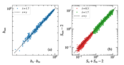
Figure 1: Numerical check of assumptions used in our theoretical analysis. (a) Factorization of the probability that an outbreak initiated at two randomly chosen adjacent nodes $(n,m)$ is finite. (b) Assumption about the average size of finite outbreaks of an outbreak initiated at two randomly chosen adjacent nodes. Results correspond to networks with degree exponent $\gamma=2.25$ and size $N=10^{4}$.

As a preliminary step, we have checked in numerical simulations the validity of the factorization for the probability $c_{nm}(t)$ that an outbreak starting from two adjacent seed nodes $(n,m)$ lasts a time smaller than or equal to $t$. To arrive at Eq. (3) it was assumed the factorization $c_{nm}(t)=c_{n}(t)c_{m}(t)$. Considering the limit of infinite time, this factorization implies that $b_{nm}=b_{n}b_{m}$, i.e., the probability of an outbreak starting with a pair of nodes being finite is equal to the product of the probabilities that each node induces independently a finite outbreak. The validity of this factorization is checked numerically in Fig. 1(a). Additionally, in the calculation of the average outbreak size, a second assumption was made, namely that the average size $S_{nm}$ of a finite outbreak starting from a pair of infected nodes $(n,m)$ is equal to sum of the average sizes of finite outbreaks starting independently from $n$ and $m$, namely, $S_{nm}=S_{n}+S_{m}$. This assumption is numerically checked in Fig. 1(b). These two results support the validity of the theoretical approach developed in the previous Section.

III.1 $\gamma=2.25$

Figure 2 compares the probability $b_{n}$ to observe a finite outbreak starting from seed $n$, measured in simulations, with the predicted value given by Eq. (4). The agreement is excellent, except for the smallest value of $\lambda$. This discrepancy is a consequence of the fact that the effective threshold for finite size is larger than its asymptotic value $\lambda_{c}=1$: hence for $\lambda=1.1$ the theory predicts $b_{n}<1$ while for most seeds $b_{n}=1$, as the system is below the effective threshold. This interpretation is confirmed by the inset, where the average value $\left\langle{b}\right\rangle=N^{-1}\sum_{n}b_{n}$ is plotted against $\lambda$: $\left\langle{b}\right\rangle$ follows well the theoretical prediction, valid in the thermodynamic limit, only for $\lambda-1>0.2$.

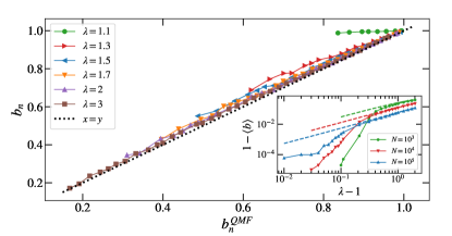
Figure 2: Numerical results for the probability $b_{n}$ in networks with degree exponent $\gamma=2.25$ and size $N=10^{4}$. Main plot: Comparison of $b_{n}$ vs the theoretical prediction $b_{n}^{QMF}$ obtained from Eq. (4) for different values of $\lambda=\alpha\Lambda_{M}$. Inset: Comparison of the average $1-\left\langle{b}\right\rangle$ vs the theoretical prediction from Eq. (4) as a function of $\lambda$.

In Fig. 3 we report the comparison between simulations and theory concerning the duration of finite outbreaks, for both subcritical and supercritical values of the parameter $\lambda$. Also in this case the agreement is fully satisfactory, the only limited discrepancies occurring around the transition, as expected.

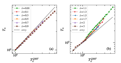
Figure 3: Comparison of the numerically evaluated average duration of finite outbreaks $T_{n}$ vs the theoretical prediction $T_{n}^{QMF}$ obtained from Eqs. (7) and (6) in networks with degree exponent $\gamma=2.25$ and size $N=10^{4}$. (a) Theoretical subcritical regime $\lambda<1$. (b) Theoretical supercritical regime $\lambda>1$.

A very good agreement is found also in Fig. 4, where the average size of finite outbreaks starting in node $n$ is compared with the solution of Eq. (21).

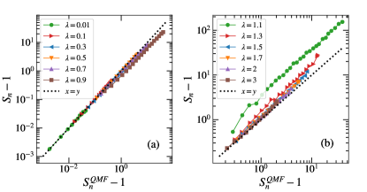
Figure 4: Comparison of the numerically evaluated average size of finite outbreaks $S_{n}$ vs the theoretical prediction $S_{n}^{QMF}$ (from Eq. (21)) in networks with degree exponent $\gamma=2.25$ and size $N=10^{4}$. (a) Theoretical subcritical regime $\lambda<1$. (b) Theoretical supercritical regime $\lambda>1$.

We conclude that the theoretical approach presented above describes very accurately the spreading influence of nodes in random uncorrelated networks with $\gamma<5/2$.

One might wonder whether a similar good agreement between theory and simulations could have been achieved by using the theory for discrete time SIS dynamics presented in Ref. [10]. We notice that the result for the average size of finite outbreaks is identical in continuous and discrete time in the subcritical regime; however, this is a coincidence that does not happen for the other observables and in the supercritical region. As an example, Fig. 5 shows the strong difference between the numerical probability $b_{n}$ to observe a finite avalanche and the corresponding discrete time prediction. This plot confirms that taking into account the continuous time nature of the dynamics is necessary for correctly predicting the spreading influence.

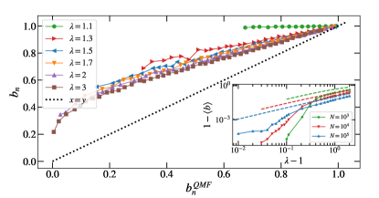
Figure 5: Numerical results for the probability $b_{n}$ in networks with degree exponent $\gamma=2.25$ and size $N=10^{4}$. Main plot: Comparison of $b_{n}$ vs the theoretical prediction $b_{n}^{QMF}$ obtained from the discrete time theory [10] for different values of $\lambda=\alpha\Lambda_{M}$. Inset: Comparison of the average $1-\left\langle{b}\right\rangle$ vs the theoretical prediction for discrete time [10] as a function of $\lambda$.

III.2 $\gamma=3.5$

As mentioned above, for $\gamma=3.5$ we do not expect a perfect agreement between theory and simulations, because of the known shortcomings of QMF theory for these mildly heterogeneous networks. This is confirmed by Fig. 6. The probability to originate a finite outbreak starting from node $n$ is definitely larger than the theoretical prediction given by Eq. (4). Only for strongly supercritical cases ($\lambda\geq 3$) the discrepancy becomes small. This is a consequence of the fact that the effective threshold in simulations is much larger than $\lambda_{c}=1$ (see the inset). At variance with the $\gamma<5/2$ case, the disagreement becomes even larger as $\lambda$ grows.

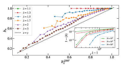
Figure 6: Numerical results for the probability $b_{n}$ in networks with degree exponent $\gamma=3.50$ and size $N=10^{4}$. Main plot: Comparison of $b_{n}$ vs the theoretical prediction $b_{n}^{QMF}$ obtained from Eq. (4) for different values of $\lambda=\alpha\Lambda_{M}$. Inset: Comparison of the average $1-\left\langle{b}\right\rangle$ vs the theoretical prediction from Eq. (4) as a function of $\lambda$.

The qualitative difference with the case $\gamma=2.25$ discussed above is apparent also in the comparison between theoretical and numerical results for the average duration of finite outbreaks, see Fig. 7. While for strongly subcritical values of $\lambda$ the agreement is reasonably good, the performance of the theory is reduced close to $\lambda_{c}$ and in a large interval of $\lambda$ values above it.

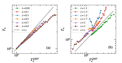
Figure 7: Comparison of the numerically evaluated average duration of finite outbreaks $T_{n}$ vs the theoretical prediction $T_{n}^{QMF}$ evaluated from Eqs. (7) and (6) in networks with degree exponent $\gamma=3.50$ and size $N=10^{4}$. (a) Theoretical subcritical regime $\lambda<1$. (b) Theoretical supercritical regime $\lambda>1$.

This is even more evident when finite outbreak average sizes are considered, see Fig. 8.

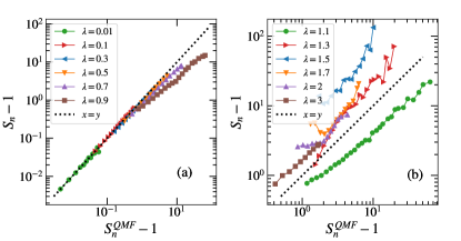
Figure 8: Comparison of the numerically evaluated average size of finite outbreaks $S_{n}$ vs the theoretical prediction $S_{n}^{QMF}$ evaluated from Eq. (21) in networks with degree exponent $\gamma=3.50$ and size $N=10^{4}$. (a) Theoretical subcritical regime $\lambda<1$. (b) Theoretical supercritical regime $\lambda>1$.

Although it is clear that QMF theory implies a systematic miscalculation of the spreading influence in this regime of $\gamma$ values, it is remarkable that for networks of this size errors are not exceedingly large. While we know that for larger systems the inaccuracy would be larger, still the theory can be taken as a fair approximation for not too small networks.

We conclude this section by answering to a question that naturally arises due to the plurality of observables quantifying spreading influence for SIS: Do all definitions identify the same nodes as more influentials? In Fig. 9 we plot the duration $T_{n}$ and size $S_{n}$ as a function of the probability $b_{n}$ to have a finite outbreak, for $\gamma=2.25$ and various values of $\lambda>1$.

Figure 9: Theoretically predicted average duration (left) and size (right) of finite outbreaks vs probability of having a finite outbreak $b_{n}$ in networks with degree exponent $\gamma=2.25$ and size $N=10^{4}$. (a) and (b):$\lambda=1.3$; (c) and (d):$\lambda=2$; (e) and (f):$\lambda=3$; (g) and (h):$\lambda=6$

We see that for small $\lambda$, $T_{n}$ and $S_{n}$ decrease with $b_{n}$, as expected. In this case a node originating many infinite outbreaks is also a good spreader generating large finite outbreaks. Rather surprisingly, things change for larger $\lambda$. In such a case, the nodes having high probability of giving rise to infinite outbreaks, generate shorter finite outbreaks. Hence they are good spreaders in one sense and bad ones in the other. Notice however that outbreaks in this case are minuscule.

III.3 Centralities as predictors

In the previous subsection we have shown that the QMF theoretical approach provides good predictions for the spreading influence of individual nodes in uncorrelated random networks. Hence we have a way to calculate the size of a finite outbreak or its duration, with reasonable accuracy, without actually performing simulations. Another relevant issue in this context has to do with the correlation between spreading influence and network centralities [4, 5, 19, 20, 21, 22]. Is the spreading influence of a given node predictable based on some topological property, such as degree, eigenvalue centrality or the many other centralities available on the market? We investigate this issue for the synthetic networks considered above, focusing on degree, eigenvector and K-core centralities, taking advantage of the knowledge about SIS dynamics in random networks gained in recent years.

In Fig. 10 we plot the average finite outbreak size as a function of the degree $k_{n}$ of the seed node. While there is clearly a strong correlation between the two quantities, it is evident that the correlation is far from perfect: some nodes with degree equal to the minimum $k_{\mathrm{min}}$ generate on average outbreaks larger than some nodes with degree even 10 times larger. This clearly shows that the annealed network assumption that degree completely determines the spreading properties of each node is only a rough approximation.

Figure 10: Comparison of the numerically evaluated average size of finite outbreaks $S_{n}$ vs the degree centrality $k_{n}$ in networks of size $N=10^{4}$. (a) Degree exponent $\gamma=2.25$. (b) Degree exponent $\gamma=3.50$. Simulations correspond to $\lambda=0.9$.

Fig. 11 shows instead the same $S_{n}$ values as a function of the eigenvector (EV) centrality $\nu_{n}$, defined as the component on node $n$ of the principal eigenvector of the adjacency matrix [23]. From this plot it appears that, in the case $\gamma=2.25$, the EV centrality is a better predictor of spreading influence than degree. We can estimate quantitatively the accuracy of both predictions by calculating the linear correlation coefficient $R$ between $S_{n}$ and the corresponding centrality. The values $R=0.952$, found for degree, and $R=0.982$, for EV centrality, indicate the superior performance of the latter.

Figure 11: Comparison of the numerically evaluated average size of finite outbreaks $S_{n}$ vs the eigenvector centrality $\nu_{n}$ in networks of size $N=10^{4}$. (a) Degree exponent $\gamma=2.25$. (b) Degree exponent $\gamma=3.50$. Simulations correspond to $\lambda=0.9$. Networks used are the same as in Fig. 10.

For $\gamma=3.5$ EV centrality is still correlated with $S_{n}$, but the presence of some structure clearly emerges. Actually, this plot can be interpreted based on the physical picture of the SIS transition sketched above. For $\gamma=3.5$ the principal eigenvector is localized around the largest hub in the network and its components decay as a function of the distance from it [16]. This explains the vertical bands occurring in the right side of the plot, corresponding to nodes at distance 1, 2, 3 from the hub .

A node with $k=k_{\mathrm{min}}$ at distance 1 from the hub is a much better spreader than a very distant node, even if much more connected. This is very clearly seen if we plot, as in Ref. [4], $S_{n}$ as a function of the degree and of the distance from the largest hub in the network, see Fig. 12(a).

Figure 12: Dependence of the average size $S_{n}$ of finite outbreaks generated as a function of the centrality properties of the seed node. (a) $S_{n}$ as a function of the degree $k_{n}$ and distance from the hub $d_{h}$ in a network of degree exponent $\gamma=3.50$. (b) $S_{n}$ as a function of the degree $k_{n}$ and the coreness $k_{s}$, defined as the K-core index of the node in the K-core decomposition, in a network of degree exponent $\gamma=2.25$. Simulations performed at $\lambda=0.9$. Networks used are the same as in Fig. 10.

Figure 13: Dependence of the probability $1-b_{n}$ to generate an infinite outbreak (i.e. a steady state) as a function of the centrality properties of the seed node. (a) $1-b_{n}$ as a function of the degree $k_{n}$ and distance from the hub $d_{h}$ in a network of degree exponent $\gamma=3.50$. (b) $1-b_{n}$ as a function of the degree $k_{n}$ and the coreness $k_{s}$ in a network of degree exponent $\gamma=2.25$. Network and simulation parameters as in Fig. 12.

It is clear that, while the spreading influence depends on the degree, there is also a clear dependence on the distance from the network hub. Nodes with the same degree are much better spreaders if they are close to the node with highest degree. For $\gamma<5/2$ we know instead that a central role in SIS dynamics is played by the mutually interconnected subgraph identified by the maximum core index in the K-core decomposition. Figure 12(b) nicely confirms this interpretation. In Fig. 13 we present an analogous analysis, performed in this case on the probability $1-b_{n}$ to generate an infinite outbreak. The correlations with $k_{n}$ and $k_{s}$ are now slightly weaker than for the average finite outbreak size, but the figure still shows that these centralities are rather good predictors for the emergence of a steady state from an infection seeded in a single node.

IV Real-world networks

So far we have considered random uncorrelated synthetic networks, whose topological properties are well controlled and suitable for performing analytical calculations, but far from those found in the real-world, where correlations, short loops, communities and other mesostructures abound [24]. The theory developed above can nevertheless be applied to any type of network. Is it able to accurately predict $b_{n}$, $T_{n}$ and $S_{n}$ for SIS dynamics on real-world structures? If not, what are the topological features that invalidate it?

We have tested the prediction accuracy of our theory on a set of real-world networks, selected from the list considered in Ref. [25]. Due to the substantial amount of computer time needed to run simulations in large networks, we focus on 20 topologies with size between 4000 and 20000 nodes. As expected the performance of our theory varies considerably depending on the topology upon which SIS dynamics occurs. In some cases, the agreement between theory and numerics is remarkably good. This is the case of the Tennis network (see Fig. 14), which indeed turns out to be rather uncorrelated and unclustered.

Figure 14: Numerical results for the Tennis real network. (a) $1-\left\langle{b}\right\rangle$ as a function of $\lambda$; (b) Numerical $b_{n}$ vs the theoretical prediction; (c) and (d) Average outbreak duration of finite outbreaks $T_{n}$ vs the theoretical prediction in the subcritical and supercritical regimes, respectively; (e) and (f) Average outbreak size of finite outbreaks $S_{n}$ vs the theoretical prediction in the subcritical and supercritical regimes, respectively.

At the other end of the spectrum is the GR-QC network, Fig. 15, which instead exhibits strong violations of our predictions.

Figure 15: Numerical results for the GR-QC real network. (a) $1-\left\langle{b}\right\rangle$ as a function of $\lambda$; (b) Numerical $b_{n}$ vs the theoretical prediction; (c) and (d) Average outbreak duration of finite outbreaks $T_{n}$ vs the theoretical prediction in the subcritical and supercritical regimes, respectively; (e) and (f) Average outbreak size of finite outbreaks $S_{n}$ vs the theoretical prediction in the subcritical and supercritical regimes, respectively.

More systematically, we have investigated for all 20 networks considered the agreement between the predicted value $S_{n}^{QMF}$ for the average size of finite outbreaks and the outcome $S_{n}$ of numerical simulations. We measure the accuracy of the prediction by evaluating for each network the average mean relative error of the prediction (MRE), defined as

$$MRE=\frac{1}{N}\sum_{n}\left|\frac{S_{n}}{S_{n}^{QMF}}-1\right|,$$ (22)

and correlating it with two typical topological properties present in real networks but absent in synthetic uncorrelated ones. We consider in particular the assortativity coefficient $r$, used to measure two-node degree correlations [26, 27], and the average clustering coefficient $c$, measuring the density of triangles in the network, and thus its departure from the tree-like assumption [28].

Because of the sampling error, the $MRE$ has a finite expected value even if the theory is exact (see Appendix D). However, by increasing the number of sampling averages it is possible to discriminate whether the measured $MRE$ is truly finite or just apparently so because of insufficient statistics.

Figure 16: Mean relative error $MRE$ observed in the set of 20 real networks as a function of the assortativity coefficient $r$, for $\lambda=0.7$ and increasing number of realizations: (a) $N_{r}=10^{3}$; (b) $N_{r}=10^{4}$; (c) $N_{r}=10^{5}$. The vertical dashed lines denote the expected value, Eq. (LABEL:expMRE), assuming that the theory is exact.

In Fig. 16 we report the values of the $MRE$ in real networks as a function of the assortativity coefficient $r$. It turns out that $N_{r}=10^{4}$ is sufficient to reach stationary MRE values. More importantly, it is apparent that the average error of the prediction decreases with increasing $r$. This means that in disassortative networks, corresponding to $r<0$, in which large degree nodes are preferentially connected to small degree nodes and viceversa [26], the average error is larger, although still limited ($<7\%$). On the other hand, for assortative networks, with $r>0$, in which nodes tend to connect with other nodes with similar degree, the average error is practically vanishing. For supercritical values of $\lambda$ (see Fig. 17) , instead, an opposite behavior emerges. The errors tend to vanish for disassortative networks while they remain quite large for many networks with positive $r$.

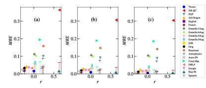
Figure 17: Mean relative error $MRE$ observed in the set of 20 real networks as a function of the assortativity coefficient $r$, for $\lambda=3$ and increasing number of realizations: (a) $N_{r}=10^{3}$; (b) $N_{r}=3\times 10^{3}$; (c) $N_{r}=10^{4}$. The vertical dashed lines denote the expected value $MRE_{th}$ assuming that the theory is exact.

In order to explore more deeply the effects of degree correlations, we consider random networks with given degree distribution and degree correlations, generated according to the Weber-Porto (WP) [29] prescription.

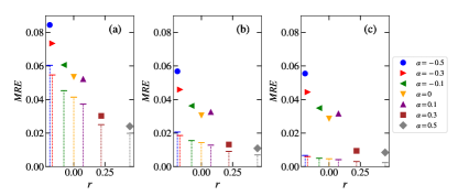
Figure 18: Mean relative error $MRE$ observed in Weber-Porto networks as a function of the assortativity coefficient $r$, for $\lambda=0.7$ and increasing number of realizations: (a) $N_{r}=10^{3}$; (b) $N_{r}=10^{4}$; (c) $N_{r}=10^{5}$. The vertical dashed lines denote the expected value $MRE_{th}$ assuming that the theory is exact. Networks used have size $N=10^{4}$ and degree exponent $\gamma=2.25$.

In this model, degree correlations are defined in terms of the average degree of the nearest neighbors of nodes of degree $k$, $\bar{k}_{nn}(k)$, which is an increasing function for assortative correlations and a decreasing one for disassortative ones [30]. Choosing a form $\bar{k}_{nn}(k)\sim k^{\alpha}$, where $\alpha<0$ ($\alpha>0$) corresponds to disassortative (assortative) networks, we find for the subcritical case the results shown in Fig. 18. As we can see, WP networks in the subcritical regime behave in a manner analogous to real networks, with a MRE decreasing with increasing $r$.

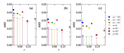
Figure 19: Mean relative error $MRE$ observed in Weber-Porto networks as a function of the assortativity coefficient $r$, for $\lambda=3$ and increasing number of realizations: (a) $N_{r}=10^{3}$; (b) $N_{r}=3\times 10^{3}$; (c) $N_{r}=10^{4}$. The vertical dashed lines denote the expected value $MRE_{th}$ assuming that the theory is exact. Networks used have size $N=10^{4}$ and degree exponent $\gamma=2.25$.

In the supercritical regime, on the other hand (see Fig. 19), the relative errors are practically independent of correlations. This observation is not in agreement with the phenomenology observed in real networks.

Finally, in Fig. 20 we report the values of MRE as a function of the average clustering coefficient $c$ in our set of real networks. In this case, no clear dependence on $c$ can be identified. These results suggest that the presence of strong disassortative degree correlations reduces the performance of our theory while other topological features (different from local clustering) are responsible for the other discrepancies between our theory and numerical simulations in real networks.

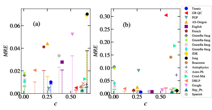
Figure 20: Mean relative error $MRE$ observed in the set of 20 real networks as a function of the clustering coefficient $c$, for $N_{r}=10^{4}$ and $\lambda=0.7$ (left), $\lambda=3$ (right). The vertical dashed lines denote the expected value $MRE_{th}$ assuming that the theory is exact

It is important to remark that the values of MRE indicate nevertheless a rather impressive overall accuracy of the theory. The relative error is smaller than $20\%$ for all networks but one (for which is a still acceptable $31\%$), indicating that even in real-world networks, with all their intricacies, our prediction is a good baseline for estimating the spreading influence of individual nodes.

V Conclusions

In this paper we have developed a theory that allows to calculate, for each single node $n$ in a network, the probability that a continuous-time SIS outbreak started in $n$ remains finite, its average duration and size. The theoretical treatment is based on a QMF-type approach to SIS dynamics and hence it shares strengths and weaknesses with the latter. For strongly heterogeneous uncorrelated networks with degree exponent $\gamma<5/2$ the theory works very well and is asymptotically exact for large networks. For $\gamma>5/2$ instead it constitutes only an approximation, whose accuracy is good only for not too large systems. The nontrivial features of the SIS epidemic transition, even on uncorrelated networks, result in a dependence of the spreading influence on topological features different from the simple degree centrality: Depending on the value of the degree exponent $\gamma$ the K-core index or the distance from the largest hub play a relevant role. When applied to SIS dynamics on real-world networks our theory turns out to be rather surprisingly accurate, with deviations from it more related to degree-correlations than to clustering.

When assessing the validity of the present approach it is to be remarked that we are able to make reasonably precise predictions for the values of the observables, with no fitting parameter to be adjusted. This is to be contrasted with many other approaches for the identification of influential spreaders for SIR dynamics, where the (much more limited) goal is the assessment of whether a node is a better spreader than another, with no prediction for the actual outbreak size or duration.

Despite this success, there is clearly still room for improvement. A first avenue of research should attempt to improve the theory in order to better predict the behavior for uncorrelated networks with $\gamma>5/2$. Theories slightly improving on QMF, such as pair-quenched mean-field [31], have been proposed, but in order to fully capture the complexity of the SIS epidemic transition for $\gamma>5/2$ one has to consider a long-range percolation process [17], which appears not easily applicable to the calculation of the spreading influence.

The other natural continuation of the present research is in the direction of better understanding spreading influence for real-world networks. It is likely that progress in this direction will require the consideration of other suitable synthetic network models, allowing to understand one at a time the effect of the various topological properties.

Appendix A Fixed points of $\mathbf{b_{n}}$

In order to study the possible steady state values of the probability $b_{n}$, we perform a linear stability analysis of the differential equation Eq. (3). The constant value $b_{n}=1$ is always a solution of Eq. (3). Let us assume a small variation from this value, defined as $c_{n}(t)=1-\epsilon_{n}(t)$. Introducing this expression into Eq. (3) and keeping only the lowest order terms, we find

$$\frac{d\epsilon_{n}(t)}{dt}\simeq-\mu\epsilon_{n}(t)+\beta\sum_{m}a_{nm}\epsilon_{m}(t)=\sum_{m}L_{nm}\epsilon_{m}(t)$$ (23)

defining the Jacobian matrix

$$L_{nm}=-\mu\delta_{nm}+\beta a_{nm}.$$ (24)

The solution $b_{n}=1$ is stable if the largest eigenvalue of the Jacobian matrix is negative. Given its structure, we can readily see that the eigenvectors of the adjacency matrix are also eigenvectors of $L_{nm}$, with an associated eigenvalue $\Lambda_{L}=-\mu+\beta\Lambda_{A}$. The largest eigenvalue of $L_{nm}$ is thus $-\mu+\beta\Lambda_{M}$, and the condition for the stability of the solution $b_{n}=1$ is

$$-\mu+\beta\Lambda_{M}<0\quad\Rightarrow\quad\frac{\beta}{\mu}\Lambda_{M}\equiv\lambda<1.$$ (25)

For $\lambda>1$ the solution $b_{n}=1$ becomes unstable, and the steady state is given by the new stable solution $b_{n}<1$ obtained from the recursive relation Eq. (4).

Appendix B Unphysical nature of the linear approximation for the average outbreak time

The linear approximation for the quantity $f_{n}(t)=b_{n}-c_{n}(t)$, obtained by neglecting the quadratic terms in Eq. (7), takes the form in rescaled time

$$\frac{df^{L}_{n}(t)}{dt}=-\frac{f^{L}_{n}(t)}{b_{n}}+\alpha b_{n}\sum_{m}a_{nm}f^{L}_{m}(t),$$ (26)

where $\alpha=\beta/\mu$. By its very definition, the probability $c_{n}(t)$ must be an increasing function in the interval $[0,\infty]$. Consequently, the function $f_{n}(t)$ must be a decreasing function in the same interval, that is, $\frac{f_{n}(t)}{dt}<0$ for $t\geq 0$, and, with the initial condition $f_{n}(0)=b_{n}$, we must have $f_{n}(t)\leq b_{n}$ for $t\geq 0$.

From Eq. (26), we can compute the slope of the function $f^{L}_{n}(t)$ at time $t=0$ given by

$$\frac{df^{L}_{n}(0)}{dt} = -\frac{f^{L}_{n}(0)}{b_{n}}+\alpha b_{n}\sum_{m}a_{nm}f^{L}_{m}(0)$$ (27)

$$= -1+\alpha b_{n}\sum_{m}a_{nm}b_{m}$$

$$= b_{n}(1+\alpha k_{n})-2,$$

where we have used the steady state condition Eq. (4). From Eq. (27) we can see that, for nodes that fulfill the condition

$$b_{n}>\frac{2}{1+\alpha k_{n}}$$ (28)

$f^{L}_{n}(t)$ is an initially increasing function with positive derivative, taking at short times values larger than $b_{n}$. This situation is completely unphysical, since it would imply that the probability $c_{n}(t)$ is negative. We therefore conclude that the linearized equation for $f_{n}(t)$ is unphysical, and cannot be used to compute the average outbreak size. This is the situation, in particular, of nodes with large degree.

In Fig. 21 we report the results of the numerical integration of the linealized equation, compared with the numerical integration of the full nonlinear equation Eq. (7). As we can see, for large values of the degree, the linearized function $f^{L}_{n}(t)$ shows a characteristic maximum in the vicinity of $t=0$, which is absent in the full non-linear solution.

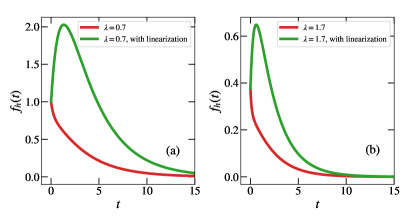
Figure 21: Full function $f_{n}(t)$ and its analogous from the linear approximation $f_{n}^{L}(t)$ numerically computed for the hub (node with maximum degree) in a network of size $N=10^{4}$ and degree exponent $\gamma=2.25$. (a) Subcritical regime, with $f_{h}(0)=1$. (b) Supercritical regime, with $f_{h}(0)=b_{n}<1$.

Appendix C The distinction between finite and infinite outbreaks in simulations

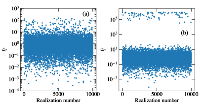
Figure 22: Total outbreak duration $T_{f}$ in many realizations of the outbreak process in network with $\gamma=2.25$, $N=10^{4}$, $\lambda=1.1$ (left panel) and $\lambda=1.3$ (right panel).

Since we are dealing with simulations in finite size systems we must decide a criterion to distinguish (above the epidemic threshold) between truly finite outbreaks (upon which we are performing averages) and outbreaks which would give rise to the stationary state in an infinite system, but that, in the finite networks we consider, end only because of fluctuations. In order to determine such a criterion, we look at the total duration $t_{f}$ of outbreaks for several realizations of the epidemic process, see Fig. 22. While close to the transition the distribution of $t_{f}$ is singly-peaked, if $\lambda$ is increased two well separated components appear, one corresponding to small values of $t_{f}$, which represent truly finite outbreaks, and the other for extremely large values of $t_{f}$, that we can associate to putatively infinite outbreaks that are stopped only due to finite size effects. In the presence of this gap, it is possible to define a maximum duration $T$, located between the two clusters of points, to distinguish the two types of outbreaks. A duration $t_{f}<T$ implies a finite outbreak, while $t_{f}\geq T$ means that the outbreak must be considered infinite. In view of Fig. 22, we set $T=100$ throughout all simulations reported in the paper. For larger values of $N$, clearly it would be possible to operate the distinction even for values of $\lambda$ closer to 1, at the price of increasing $T$ and hence the simulation time.

Appendix D Expected value of the $MRE$

When comparing simulations with theory, even in the case the latter is exact, i.e., the expected value of the outbreak size is $S_{n}^{QMF}$, sampling error implies that the $MRE$ (Eq. (22)) has a finite value depending on the number of realizations considered. Indeed, for $N_{r}$ realizations, from the central limit theorem

$$S_{n}=S_{n}^{QMF}+\eta_{n}$$ (29)

where $\eta_{n}$ is a Gaussian $P(\eta_{n})$ of zero mean and variance $\sigma_{n}^{2}/N_{r}$, with $\sigma_{n}^{2}$ the variance of outbreak size distribution for given $n$. Then the expected $MRE$ value is

$$MRE_{th} = \frac{1}{N}\sum_{n}\frac{1}{S_{n}^{QMF}}\int_{-\infty}^{+\infty}d\eta_{n}P(\eta_{n})|\eta_{n}|$$

$$= \frac{2}{N}\sum_{n}\frac{1}{S_{n}^{QMF}}\int_{0}^{\infty}d\eta_{n}P(\eta_{n})\eta_{n}$$

$$= \frac{2}{\sqrt{2\pi N_{r}}}\frac{1}{N}\sum_{n}\frac{\sigma_{n}}{S_{n}^{QMF}}$$

Therefore, by increasing $N_{r}$ it is possible to discriminate whether the measured $MRE$ is truly finite or just because of insufficient statistics.